An efficient dynamical low-rank algorithm
for the Boltzmann–BGK equation
close to the compressible viscous flow regime111 JH’s research was supported in part by NSF CAREER grant DMS-1654152 and NSF CDS&E grant CBET-1854829. LY’s research was supported in part by NSF DMS grant DMS-1818449.

Lukas Einkemmer222Department of Mathematics, University of Innsbruck, Innsbruck, A-6020, Austria (lukas.einkemmer@uibk.ac.at).,  Jingwei Hu333Department of Mathematics, Purdue University, West Lafayette, IN 47907, USA (jingweihu@purdue.edu).,  and  Lexing Ying444Department of Mathematics, Stanford University, Stanford, CA 94305, USA (lexing@stanford.edu).
Abstract

It has recently been demonstrated that dynamical low-rank algorithms can provide robust and efficient approximation to a range of kinetic equations. This is true especially if the solution is close to some asymptotic limit where it is known that the solution is low-rank. A particularly interesting case is the fluid dynamic limit that is commonly obtained in the limit of small Knudsen number. However, in this case the Maxwellian which describes the corresponding equilibrium distribution is not necessarily low-rank; because of this, the methods known in the literature are only applicable to the weakly compressible case. In this paper, we propose an efficient dynamical low-rank integrator that can capture the fluid limit – the Navier-Stokes equations – of the Boltzmann-BGK model even in the compressible regime. This is accomplished by writing the solution as f=Mg𝑓𝑀𝑔f=Mg, where M𝑀M is the Maxwellian and the low-rank approximation is only applied to g𝑔g. To efficiently implement this decomposition within a low-rank framework requires, in the isothermal case, that certain coefficients are evaluated using convolutions, for which fast algorithms are known. Using the proposed decomposition also has the advantage that the rank required to obtain accurate results is significantly reduced compared to the previous state of the art. We demonstrate this by performing a number of numerical experiments and also show that our method is able to capture sharp gradients/shock waves.

Key words. dynamical low-rank integrator, Boltzmann-BGK model, compressible Navier-Stokes equations, Chapman-Enskog expansion, convolution, Fourier spectral methods.

AMS subject classifications. 35Q20, 35Q30, 65L04, 65M99.

1 Introduction

The Navier-Stokes (NS) equations are widely used in many scientific and engineering disciplines and its fundamental importance cannot be underestimated. Nevertheless, it is increasingly realized that the NS equations may not provide an accurate description when the underlying system is not dense enough to be in thermodynamic equilibrium (i.e., when there is a significant deviation from the Maxwellian distribution). This is especially true when the mean free path is comparable to the characteristic length, a situation that occurs, e.g., in the atmosphere at high altitude or in micro-devices. To accurately describe such rarefied or transitional flows, the kinetic Boltzmann equation should be used [6]. However, this comes at the price of solving a six-dimensional equation in phase space. Although significant progress has been made in the past decades to solve Boltzmann type kinetic equations more accurately and efficiently (see for instance [9]), the high-dimensional nature of such equations still poses a challenging problem in scientific computing. It is therefore the goal of this paper to introduce an efficient method for the kinetic BGK equation in a wide range of flow regimes whose computational cost is comparable to solving the macroscopic fluid equations.

The BGK equation, initially proposed by Bhatnagar, Gross, and Krook [5], is one of the widely used kinetic models as it is much simpler than the full Boltzmann equation yet possesses most of its key properties. In dimensionless form, the equation reads

tf+vxf=νε(Mf),t>0,xΩdx,vdv,formulae-sequenceformulae-sequencesubscript𝑡𝑓𝑣subscript𝑥𝑓𝜈𝜀𝑀𝑓formulae-sequence𝑡0𝑥Ωsuperscriptsubscript𝑑𝑥𝑣superscriptsubscript𝑑𝑣\partial_{t}f+v\cdot\nabla_{x}f=\frac{\nu}{\varepsilon}(M-f),\quad t>0,\quad x\in\Omega\subset\mathbb{R}^{d_{x}},\quad v\in\mathbb{R}^{d_{v}}, (1.1)

where f=f(t,x,v)𝑓𝑓𝑡𝑥𝑣f=f(t,x,v) is the one-particle probability density function depending on time t𝑡t, position x𝑥x, and velocity v𝑣v. The so-called Maxwellian M𝑀M is defined as

M(t,x,v)=ρ(t,x)(2πT(t,x))dv/2exp(|vu(t,x)|22T(t,x))𝑀𝑡𝑥𝑣𝜌𝑡𝑥superscript2𝜋𝑇𝑡𝑥subscript𝑑𝑣2superscript𝑣𝑢𝑡𝑥22𝑇𝑡𝑥M(t,x,v)=\frac{\rho(t,x)}{(2\pi T(t,x))^{d_{v}/2}}\exp\left(-\frac{|v-u(t,x)|^{2}}{2T(t,x)}\right) (1.2)

with the density ρ𝜌\rho, bulk velocity u𝑢u, and temperature T𝑇T given by the moments of f𝑓f:

ρ=dvfdv,u=1ρdvvfdv,T=1dvρdv|vu|2fdv.formulae-sequence𝜌subscriptsuperscriptsubscript𝑑𝑣𝑓differential-d𝑣formulae-sequence𝑢1𝜌subscriptsuperscriptsubscript𝑑𝑣𝑣𝑓differential-d𝑣𝑇1subscript𝑑𝑣𝜌subscriptsuperscriptsubscript𝑑𝑣superscript𝑣𝑢2𝑓differential-d𝑣\rho=\int_{\mathbb{R}^{d_{v}}}f\,\mathrm{d}{v},\quad u=\frac{1}{\rho}\int_{\mathbb{R}^{d_{v}}}vf\,\mathrm{d}{v},\quad T=\frac{1}{d_{v}\rho}\int_{\mathbb{R}^{d_{v}}}|v-u|^{2}f\,\mathrm{d}{v}. (1.3)

The viscosity ν𝜈\nu is a function of ρ𝜌\rho and T𝑇T; typically, one assumes ν=ρT1ω𝜈𝜌superscript𝑇1𝜔\nu=\rho T^{1-\omega} with 0.5ω10.5𝜔10.5\leq\omega\leq 1. Finally, ε𝜀\varepsilon is the Knudsen number, defined as the ratio of the mean free path and the chosen characteristic length scale. The value of ε𝜀\varepsilon indicates the flow regime [37] (see Section 2 for more details): 1) ε0𝜀0\varepsilon\rightarrow 0, Euler regime (the flow is well described by the compressible Euler equations; 2) 0<ε0.010𝜀less-than-or-similar-to0.010<\varepsilon\lesssim 0.01, NS regime (the flow is well described by the compressible NS equations); and 3) 0.01ε1less-than-or-similar-to0.01𝜀less-than-or-similar-to10.01\lesssim\varepsilon\lesssim 1, transition regime (the NS equations fail, and one has to resort to extended macroscopic models or the original kinetic equation (1.1)).

In practical applications we often have dx=dv=3subscript𝑑𝑥subscript𝑑𝑣3d_{x}=d_{v}=3, hence the computational cost of solving (1.1) would be at least 𝒪(N6)𝒪superscript𝑁6\mathcal{O}(N^{6}), where N𝑁N is the number of mesh points in each dimension of the physical and velocity space. To reduce this cost, we are going to adopt the basic framework of so-called dynamical low-rank projection, which has a long history in quantum dynamics; see, for example, [33, 32] for the MCTDH approach to molecular quantum dynamics in the chemical physics literature and [27, 28, 7] for a mathematical point of view. In a general mathematical setting, the dynamical low-rank approximation has been studied in [21, 22, 30, 2]. A major algorithmic advance for the time integration was achieved with the projector-splitting method first proposed in [29]. In contrast to standard time-stepping methods, the projector-splitting method is robust to the presence of small singular values in the low-rank approximation [20]. Recently, this method has been applied to several kinetic equations including the Vlasov equation [13, 14, 15], the BGK equation (in the weakly compressible regime) [11], and radiative transport equations [35, 10, 12].

Though the details vary for each of the aforementioned equations, the common idea is to seek a low-rank approximation of the unknown function f𝑓f as

f(t,x,v)i,j=1rXi(t,x)Sij(t)Vj(t,v),𝑓𝑡𝑥𝑣superscriptsubscript𝑖𝑗1𝑟subscript𝑋𝑖𝑡𝑥subscript𝑆𝑖𝑗𝑡subscript𝑉𝑗𝑡𝑣f(t,x,v)\approx\sum_{i,j=1}^{r}X_{i}(t,x)S_{ij}(t)V_{j}(t,v), (1.4)

where r𝑟r is the rank, {Xi}subscript𝑋𝑖\{X_{i}\} and {Vj}subscript𝑉𝑗\{V_{j}\} are the orthonormal bases in the physical space and velocity space, respectively. The dynamics of Xisubscript𝑋𝑖X_{i}, Sijsubscript𝑆𝑖𝑗S_{ij} and Vjsubscript𝑉𝑗V_{j} are determined by projecting the equation onto the tangent space of the low-rank solution manifold. Upon a further operator splitting, the original six-dimensional problem can be reduced to a few three-dimensional problems. It is also clear that the efficiency of this low-rank method depends on the intrinsic rank of the underlying problem. If the solution f𝑓f has no low-rank structure, a large value of r𝑟r would be needed in (1.4) and hence the gain of the method would be marginal. For a number of linear and weakly nonlinear problems it is known that the solution is low-rank in some asymptotic limit. This is the case, for instance, in the radiative transfer/linear transport equations wherein one obtains a rank-111 solution in the diffusion limit. The asymptotic-preserving (AP) dynamical low-rank methods that can capture this behavior have been considered in [10, 12]. A similar approach was undertaken in [11] for the BGK equation, where the method is limited to the weakly compressible flows since the Maxwellian (1.2) is not necessarily low-rank.

In this work we introduce a robust dynamical low-rank integrator for the BGK equation (1.1) that is able to capture the fluid limit – the NS equations – in the compressible (isothermal) case. We do this by writing the solution as f=Mg𝑓𝑀𝑔f=Mg, where only g𝑔g is subjected to a low-rank approximation. Note that this is a drastically different decomposition compared to (1.4) due to the nonlinearity of M𝑀M. To efficiently implement this decomposition within the low-rank framework requires the evaluation of certain integrals involving the Maxwellian. If this is done naively the numerical method would suffer from excessive computational cost that scales as 𝒪(N6)𝒪superscript𝑁6\mathcal{O}(N^{6}). We demonstrate that, in the isothermal case, this difficulty can be overcome by interpreting the corresponding integrals as convolutions and using a FFT based fast convolution algorithm.

The proposed approach has several advantages. First, from the Chapman-Enskog expansion [3] we can guarantee that g𝑔g is low-rank for small values of ε𝜀\varepsilon (in both the Euler and NS regimes) for compressible problems. Second, for weakly compressible problems, the rank r𝑟r needed to obtain an accurate approximation is much smaller than that in [11] (because we only assume that g=f/M𝑔𝑓𝑀g=f/M is low-rank and do not need to perform the expansion of M𝑀M in small velocities as was done in [11]). Third, the fluid moments, such as density ρ𝜌\rho and momentum ρu𝜌𝑢\rho u, are integrated as part of the numerical scheme. Thus, using an appropriate discretization, as will be done here, conservation of mass and momentum is ensured. The algorithm is also able to handle problems with sharp gradients/shock waves. In addition, since the proposed low-rank algorithm automatically takes care of regions close to the fluid regime (the scheme becomes a consistent discretization to the NS equations when ε𝜀\varepsilon is small), it can be used to perform simulations in a wide range of flow regimes without the need to explicitly couple a kinetic solver with a fluid one (which is potentially complicated in a hybrid approach; see, e.g., [17, 8]). In that context the present scheme would be used in a similar way as the Hermite expansion in [38], with the added advantage that the computational cost of the kinetic solver is reduced dramatically.

The rest of this paper is organized as follows. In Section 2 we describe the fluid dynamic limits of the BGK equation. We then motivate the low-rank approximation used (Section 3) and derive the corresponding numerical algorithm in a semi-discrete setting (Section 4). The full discretization is discussed in Section 5. A formal analysis is performed in Section 6 to show that our numerical scheme can indeed capture the NS limit when ε𝜀\varepsilon is small. Finally we present the results of a range of numerical experiments in Section 7.

2 Fluid limits of the BGK equation

In this section, we derive the fluid dynamic limits of the BGK equation (1.1) using the Chapman-Enskog expansion [3]. We will see that the compressible Euler equations can be obtained when ε0𝜀0\varepsilon\rightarrow 0, while the compressible NS equations can be obtained when retaining 𝒪(ε)𝒪𝜀\mathcal{O}(\varepsilon) information. Although the procedure is quite standard in the kinetic literature, we have decided to include it here because our following low-rank approximation is strongly motivated by this analysis.

When ε𝜀\varepsilon is small, from (1.1), formally one has

f=M+𝒪(ε).𝑓𝑀𝒪𝜀f=M+\mathcal{O}(\varepsilon). (2.1)

Hence it makes sense to assume that

f=M+εf1,𝑓𝑀𝜀subscript𝑓1f=M+\varepsilon f_{1}, (2.2)

where f1subscript𝑓1f_{1} is an 𝒪(1)𝒪1\mathcal{O}(1) function. We then substitute (2.2) into (1.1) to obtain

f1=1ν(tf+vxf)=1ν(tM+vxM)+𝒪(ε).subscript𝑓11𝜈subscript𝑡𝑓𝑣subscript𝑥𝑓1𝜈subscript𝑡𝑀𝑣subscript𝑥𝑀𝒪𝜀f_{1}=-\frac{1}{\nu}(\partial_{t}f+v\cdot\nabla_{x}f)=-\frac{1}{\nu}(\partial_{t}M+v\cdot\nabla_{x}M)+\mathcal{O}(\varepsilon). (2.3)

On the other hand, taking the first dv+2subscript𝑑𝑣2d_{v}+2 moments of (1.1), i.e. multiplying (1.1) by ϕ(v):=(1,v,|v|2/2)Tassignitalic-ϕ𝑣superscript1𝑣superscript𝑣22𝑇\phi(v):=(1,v,|v|^{2}/2)^{T} and integrating in v𝑣v, yields

tfϕv+xvϕfv=0,v:=dvdv.formulae-sequencesubscript𝑡subscriptdelimited-⟨⟩𝑓italic-ϕ𝑣subscript𝑥subscriptdelimited-⟨⟩𝑣italic-ϕ𝑓𝑣0assignsubscriptdelimited-⟨⟩𝑣subscriptsuperscriptsubscript𝑑𝑣d𝑣\partial_{t}\langle f\phi\rangle_{v}+\nabla_{x}\cdot\langle v\phi f\rangle_{v}=0,\quad\langle\ \cdot\ \rangle_{v}:=\int_{\mathbb{R}^{d_{v}}}\cdot\ \,\mathrm{d}{v}. (2.4)

By substituting (2.2) into (2.4) we obtain

tfϕv+xvϕMv=εxvϕf1v.subscript𝑡subscriptdelimited-⟨⟩𝑓italic-ϕ𝑣subscript𝑥subscriptdelimited-⟨⟩𝑣italic-ϕ𝑀𝑣𝜀subscript𝑥subscriptdelimited-⟨⟩𝑣italic-ϕsubscript𝑓1𝑣\partial_{t}\langle f\phi\rangle_{v}+\nabla_{x}\cdot\langle v\phi M\rangle_{v}=-\varepsilon\nabla_{x}\cdot\langle v\phi f_{1}\rangle_{v}. (2.5)

Using the macroscopic quantities defined in (1.3) and

1:=dv(vu)(vu)f1dv,q1:=12dv(vu)|vu|2f1dv,formulae-sequenceassignsubscript1subscriptsuperscriptsubscript𝑑𝑣tensor-product𝑣𝑢𝑣𝑢subscript𝑓1differential-d𝑣assignsubscript𝑞112subscriptsuperscriptsubscript𝑑𝑣𝑣𝑢superscript𝑣𝑢2subscript𝑓1differential-d𝑣\mathbb{P}_{1}:=-\int_{\mathbb{R}^{d_{v}}}(v-u)\otimes(v-u)f_{1}\,\mathrm{d}{v},\quad q_{1}:=-\frac{1}{2}\int_{\mathbb{R}^{d_{v}}}(v-u)|v-u|^{2}f_{1}\,\mathrm{d}{v}, (2.6)

we can write (2.5) as

{tρ+x(ρu)=0,t(ρu)+x(ρuu+pId)=εx1,tE+x((E+p)u)=εx(1u+q1),casessubscript𝑡𝜌subscript𝑥𝜌𝑢0subscript𝑡𝜌𝑢subscript𝑥tensor-product𝜌𝑢𝑢𝑝Id𝜀subscript𝑥subscript1subscript𝑡𝐸subscript𝑥𝐸𝑝𝑢𝜀subscript𝑥subscript1𝑢subscript𝑞1\displaystyle\left\{\begin{array}[]{l}\partial_{t}\rho+\nabla_{x}\cdot(\rho u)=0,\\[8.0pt] \partial_{t}(\rho u)+\nabla_{x}\cdot(\rho u\otimes u+p\text{Id})=\varepsilon\nabla_{x}\cdot\mathbb{P}_{1},\\[8.0pt] \partial_{t}E+\nabla_{x}\cdot((E+p)u)=\varepsilon\nabla_{x}\cdot(\mathbb{P}_{1}u+q_{1}),\end{array}\right. (2.10)

where p=ρT𝑝𝜌𝑇p=\rho T is the pressure, Id is the identity matrix, and E=dv2ρT+12ρu2𝐸subscript𝑑𝑣2𝜌𝑇12𝜌superscript𝑢2E=\frac{d_{v}}{2}\rho T+\frac{1}{2}\rho u^{2} is the total energy. Neglecting the 𝒪(ε)𝒪𝜀\mathcal{O}(\varepsilon) terms, (2.10) become the compressible Euler equations.

To further derive the right hand side of (2.10), we first note that for the Maxwellian function defined in (1.2) one has

1M(tM+vxM)=1ρ(tρ+vxρ)+(vu)T(tu+vxu)+(|vu|22T2dv2T)(tT+vxT).1𝑀subscript𝑡𝑀𝑣subscript𝑥𝑀1𝜌subscript𝑡𝜌𝑣subscript𝑥𝜌𝑣𝑢𝑇subscript𝑡𝑢𝑣subscript𝑥𝑢superscript𝑣𝑢22superscript𝑇2subscript𝑑𝑣2𝑇subscript𝑡𝑇𝑣subscript𝑥𝑇\frac{1}{M}(\partial_{t}M+v\cdot\nabla_{x}M)=\frac{1}{\rho}(\partial_{t}\rho+v\cdot\nabla_{x}\rho)+\frac{(v-u)}{T}\cdot(\partial_{t}u+v\cdot\nabla_{x}u)+\left(\frac{|v-u|^{2}}{2T^{2}}-\frac{d_{v}}{2T}\right)(\partial_{t}T+v\cdot\nabla_{x}T). (2.11)

Since we already knew that ρ𝜌\rho, u𝑢u and T𝑇T satisfy the compressible Euler equations to the leading order, we can use the spatial derivatives of these functions to replace the time derivatives. This yields

1M(tM+vxM)=(|vu|22Tdv+22)(vu)xTT+((vu)(vu)T|vu|2dvTId):xu+𝒪(ε),:1𝑀subscript𝑡𝑀𝑣subscript𝑥𝑀superscript𝑣𝑢22𝑇subscript𝑑𝑣22𝑣𝑢subscript𝑥𝑇𝑇tensor-product𝑣𝑢𝑣𝑢𝑇superscript𝑣𝑢2subscript𝑑𝑣𝑇Idsubscript𝑥𝑢𝒪𝜀\frac{1}{M}(\partial_{t}M+v\cdot\nabla_{x}M)=\left(\frac{|v-u|^{2}}{2T}-\frac{d_{v}+2}{2}\right)\frac{(v-u)\cdot\nabla_{x}T}{T}+\left(\frac{(v-u)\otimes(v-u)}{T}-\frac{|v-u|^{2}}{d_{v}T}\text{Id}\right):\nabla_{x}u+\mathcal{O}(\varepsilon), (2.12)

where

σ(u):=xu+(xu)T2dv(xu)Id.assign𝜎𝑢subscript𝑥𝑢superscriptsubscript𝑥𝑢𝑇2subscript𝑑𝑣subscript𝑥𝑢Id\sigma(u):=\nabla_{x}u+(\nabla_{x}u)^{T}-\frac{2}{d_{v}}(\nabla_{x}\cdot u)\ \text{Id}. (2.13)

Note that xusubscript𝑥𝑢\nabla_{x}u is a matrix with ij𝑖𝑗ij-th component given by xjuisubscriptsubscript𝑥𝑗subscript𝑢𝑖\partial_{x_{j}}u_{i} and the operation ::: between two matrices is defined as A:B=ijaijbij:𝐴𝐵subscript𝑖𝑗subscript𝑎𝑖𝑗subscript𝑏𝑖𝑗A:B=\sum_{ij}a_{ij}b_{ij}.

Plugging (2.12) into (2.3) gives

f1=Mν[(|vu|22Tdv+22)(vu)xTT+((vu)(vu)T|vu|2dvTId):xu]+𝒪(ε).f_{1}=-\frac{M}{\nu}\left[\left(\frac{|v-u|^{2}}{2T}-\frac{d_{v}+2}{2}\right)\frac{(v-u)\cdot\nabla_{x}T}{T}+\left(\frac{(v-u)\otimes(v-u)}{T}-\frac{|v-u|^{2}}{d_{v}T}\text{Id}\right):\nabla_{x}u\right]+\mathcal{O}(\varepsilon). (2.14)

One can verify by direct integration that

1=1νρTσ(u)+𝒪(ε)=Tωσ(u)+𝒪(ε),q1=1νdv+22ρTxT+𝒪(ε)=dv+22TωxT+𝒪(ε).formulae-sequencesubscript11𝜈𝜌𝑇𝜎𝑢𝒪𝜀superscript𝑇𝜔𝜎𝑢𝒪𝜀subscript𝑞11𝜈subscript𝑑𝑣22𝜌𝑇subscript𝑥𝑇𝒪𝜀subscript𝑑𝑣22superscript𝑇𝜔subscript𝑥𝑇𝒪𝜀\begin{split}\mathbb{P}_{1}&=\frac{1}{\nu}\rho T\sigma(u)+\mathcal{O}(\varepsilon)=T^{\omega}\sigma(u)+\mathcal{O}(\varepsilon),\\ q_{1}&=\frac{1}{\nu}\frac{d_{v}+2}{2}\rho T\nabla_{x}T+\mathcal{O}(\varepsilon)=\frac{d_{v}+2}{2}T^{\omega}\nabla_{x}T+\mathcal{O}(\varepsilon).\end{split} (2.15)

Substituting the above 1subscript1\mathbb{P}_{1} and q1subscript𝑞1q_{1} into (2.10), we finally obtain

{tρ+x(ρu)=0,t(ρu)+x(ρuu+pId)=εx(μσ(u))+𝒪(ε2),tE+x((E+p)u)=εx(μσ(u)u+κxT)+𝒪(ε2),casessubscript𝑡𝜌subscript𝑥𝜌𝑢0subscript𝑡𝜌𝑢subscript𝑥tensor-product𝜌𝑢𝑢𝑝Id𝜀subscript𝑥𝜇𝜎𝑢𝒪superscript𝜀2subscript𝑡𝐸subscript𝑥𝐸𝑝𝑢𝜀subscript𝑥𝜇𝜎𝑢𝑢𝜅subscript𝑥𝑇𝒪superscript𝜀2\displaystyle\left\{\begin{array}[]{l}\partial_{t}\rho+\nabla_{x}\cdot(\rho u)=0,\\[8.0pt] \partial_{t}(\rho u)+\nabla_{x}\cdot(\rho u\otimes u+p\text{Id})=\varepsilon\nabla_{x}\cdot(\mu\sigma(u))+\mathcal{O}(\varepsilon^{2}),\\[8.0pt] \partial_{t}E+\nabla_{x}\cdot((E+p)u)=\varepsilon\nabla_{x}\cdot(\mu\sigma(u)u+\kappa\nabla_{x}T)+\mathcal{O}(\varepsilon^{2}),\end{array}\right. (2.19)

where μ:=Tωassign𝜇superscript𝑇𝜔\mu:=T^{\omega} and κ:=dv+22μassign𝜅subscript𝑑𝑣22𝜇\kappa:=\frac{d_{v}+2}{2}\mu are, respectively, the coefficients of viscosity and heat conductivity. Ignoring 𝒪(ε2)𝒪superscript𝜀2\mathcal{O}(\varepsilon^{2}) terms, (2.19) are the compressible Navier-Stokes equations.

Remark 2.1.

It is well-known that the BGK model (1.1) cannot produce the correct Prandtl number (Pr:=dv+22μκ1assignPrsubscript𝑑𝑣22𝜇𝜅1\text{Pr}:=\frac{d_{v}+2}{2}\frac{\mu}{\kappa}\equiv 1 in the BGK model while for most gases Pr<1Pr1\text{Pr}<1). To correct this defect, various models have been proposed such as the ES-BGK model [1] or the Shakhov model [36]. Since our main focus in this paper are isothermal flows, this defect is irrelevant.

3 The low-rank approximation

From the previous section we can see that when ε𝜀\varepsilon is small, f𝑓f can be expanded as (see (2.2) and (2.14)):

f=MεMν[(|vu|22Tdv+22)(vu)xTT+((vu)(vu)T|vu|2dvTId):xu]+𝒪(ε2).f=M-\varepsilon\frac{M}{\nu}\left[\left(\frac{|v-u|^{2}}{2T}-\frac{d_{v}+2}{2}\right)\frac{(v-u)\cdot\nabla_{x}T}{T}+\left(\frac{(v-u)\otimes(v-u)}{T}-\frac{|v-u|^{2}}{d_{v}T}\text{Id}\right):\nabla_{x}u\right]+\mathcal{O}(\varepsilon^{2}). (3.1)

Note that the Maxwellian M𝑀M is a normal distribution with (time and spatially dependent) mean u(t,x)𝑢𝑡𝑥u(t,x) and variance T(t,x)𝑇𝑡𝑥T(t,x), so M𝑀M is generally not a low-rank or separable function in x𝑥x and v𝑣v. Because of this, we do not directly use the low-rank approximation (1.4) for f𝑓f. Instead, we consider

f=Mg,𝑓𝑀𝑔f=Mg, (3.2)

then

g=1ε1ν[(|vu|22Tdv+22)(vu)xTT+((vu)(vu)T|vu|2dvTId):xu]+𝒪(ε2),g=1-\varepsilon\frac{1}{\nu}\left[\left(\frac{|v-u|^{2}}{2T}-\frac{d_{v}+2}{2}\right)\frac{(v-u)\cdot\nabla_{x}T}{T}+\left(\frac{(v-u)\otimes(v-u)}{T}-\frac{|v-u|^{2}}{d_{v}T}\text{Id}\right):\nabla_{x}u\right]+\mathcal{O}(\varepsilon^{2}), (3.3)

which is a low-rank function in x𝑥x and v𝑣v even at 𝒪(ε)𝒪𝜀\mathcal{O}(\varepsilon). This can be most easily seen by recognizing that the 𝒪(ε)𝒪𝜀\mathcal{O}(\varepsilon) term can be written as a sum of products of functions that depend only on x𝑥x (such as u𝑢u, 1/T1𝑇1/T, and xusubscript𝑥𝑢\nabla_{x}u) and functions that only depend on v𝑣v (such as v𝑣v, v2superscript𝑣2v^{2} and vvtensor-product𝑣𝑣v\otimes v).

This motivates us to seek an expansion of g𝑔g in the following form:

g=i,j=1rXi(t,x)Sij(t)Vj(t,v),𝑔superscriptsubscript𝑖𝑗1𝑟subscript𝑋𝑖𝑡𝑥subscript𝑆𝑖𝑗𝑡subscript𝑉𝑗𝑡𝑣g=\sum_{i,j=1}^{r}X_{i}(t,x)S_{ij}(t)V_{j}(t,v), (3.4)

where {Xi}subscript𝑋𝑖\{X_{i}\} and {Vj}subscript𝑉𝑗\{V_{j}\} are the orthonormal bases in x𝑥x and v𝑣v, respectively. Before proceeding, let us note that a multiplicative deviation from equilibrium to improve compression has been used in the context of sparse grids and the Vlasov equation [24], albeit in the somewhat simpler setting where u=0𝑢0u=0.

To track the evolution of M𝑀M, one can consider the moment equation (2.4) which we rewrite using a slightly different notation:

tU+xvϕMgv=0,subscript𝑡𝑈subscript𝑥subscriptdelimited-⟨⟩𝑣italic-ϕ𝑀𝑔𝑣0\partial_{t}U+\nabla_{x}\cdot\langle v\phi Mg\rangle_{v}=0, (3.5)

where U:=(ρ,ρu,E)Tassign𝑈superscript𝜌𝜌𝑢𝐸𝑇U:=(\rho,\rho u,E)^{T} and ϕ(v):=(1,v,|v|2/2)Tassignitalic-ϕ𝑣superscript1𝑣superscript𝑣22𝑇\phi(v):=(1,v,|v|^{2}/2)^{T}.

To track the dynamics of Xisubscript𝑋𝑖X_{i}, Sijsubscript𝑆𝑖𝑗S_{ij} and Vjsubscript𝑉𝑗V_{j}, we proceed as follows. Substituting f=Mg𝑓𝑀𝑔f=Mg into equation (1.1) yields

tg=vxg1M(tM+vxM)g+νε(1g):=h.subscript𝑡𝑔𝑣subscript𝑥𝑔1𝑀subscript𝑡𝑀𝑣subscript𝑥𝑀𝑔𝜈𝜀1𝑔assign\partial_{t}g=-v\cdot\nabla_{x}g-\frac{1}{M}(\partial_{t}M+v\cdot\nabla_{x}M)g+\frac{\nu}{\varepsilon}(1-g):=h. (3.6)

We now apply the projector-splitting based dynamical low-rank algorithm [29] to (3.6). That is, constraining g𝑔g to lie on the low-rank manifold:

tg=jVj,hvVji,jXiXiVj,hx,vVj+iXiXi,hxsubscript𝑡𝑔subscript𝑗subscriptsubscript𝑉𝑗𝑣subscript𝑉𝑗subscript𝑖𝑗subscript𝑋𝑖subscriptsubscript𝑋𝑖subscript𝑉𝑗𝑥𝑣subscript𝑉𝑗subscript𝑖subscript𝑋𝑖subscriptsubscript𝑋𝑖𝑥\partial_{t}g=\sum_{j}\langle V_{j},h\rangle_{v}V_{j}-\sum_{i,j}X_{i}\langle X_{i}V_{j},h\rangle_{x,v}V_{j}+\sum_{i}X_{i}\langle X_{i},h\rangle_{x} (3.7)

and then performing the operator splitting yields the following numerical algorithm:

– Let Kj=iXiSijsubscript𝐾𝑗subscript𝑖subscript𝑋𝑖subscript𝑆𝑖𝑗K_{j}=\sum_{i}X_{i}S_{ij}, then g=jKjVj𝑔subscript𝑗subscript𝐾𝑗subscript𝑉𝑗g=\sum_{j}K_{j}V_{j}. Update Kjsubscript𝐾𝑗K_{j} by solving

tKj=Vj,hv,subscript𝑡subscript𝐾𝑗subscriptsubscript𝑉𝑗𝑣\partial_{t}K_{j}=\langle V_{j},h\rangle_{v}, (3.8)

then perform an orthonormalization of Kjsubscript𝐾𝑗K_{j} to generate new Xisubscript𝑋𝑖X_{i} and Sijsubscript𝑆𝑖𝑗S_{ij} (using a QR decomposition).

– Update Sijsubscript𝑆𝑖𝑗S_{ij} by solving

tSij=XiVj,hx,v.subscript𝑡subscript𝑆𝑖𝑗subscriptsubscript𝑋𝑖subscript𝑉𝑗𝑥𝑣\partial_{t}S_{ij}=-\langle X_{i}V_{j},h\rangle_{x,v}. (3.9)

– Let Li=jSijVjsubscript𝐿𝑖subscript𝑗subscript𝑆𝑖𝑗subscript𝑉𝑗L_{i}=\sum_{j}S_{ij}V_{j}, then g=iXiLi𝑔subscript𝑖subscript𝑋𝑖subscript𝐿𝑖g=\sum_{i}X_{i}L_{i}. Update Lisubscript𝐿𝑖L_{i} by solving

tLi=Xi,hx,subscript𝑡subscript𝐿𝑖subscriptsubscript𝑋𝑖𝑥\partial_{t}L_{i}=\langle X_{i},h\rangle_{x}, (3.10)

then perform an orthonormalization on Lisubscript𝐿𝑖L_{i} to generate new Sijsubscript𝑆𝑖𝑗S_{ij} and Vjsubscript𝑉𝑗V_{j} (using a QR decomposition).

For the derivation of the above algorithm we refer the readers to [13] and the references contained therein. The algorithm described is robust in the sense that over approximation, i.e. small singular values in S𝑆S, do not cause any numerical issues. Furthermore, the order of the subflows (3.8)-(3.10) can be chosen freely. Any order results in a numerical method that is first order accurate (in time). For higher order methods this can be exploited to lower the overall computational cost (see, e.g., [13]).

4 The dynamical low-rank algorithm

In this section we present the proposed algorithm in detail. This includes the low-rank integrator for g𝑔g as well as the necessary numerical scheme to advance the moments in time. The present section describes a semi-discrete version where time is discretized but space is left continuous. We will consider possible spatial discretizations in more details in Section 5.

From this point onward, we will assume that the temperature is constant in order to simplify the presentation. Without loss of generality we can then choose T1𝑇1T\equiv 1. Assuming that the ideal gas law holds true, this simply means that we measure the velocity u𝑢u in fractions of the speed of sound. The rationale for this assumption lies in the fact that isothermal flows represent an interesting nontrivial compressible case that we propose to efficiently treat using fast convolution algorithms. We will discuss the non-constant temperature case in more detail in Remark 4.3 given at the end of this section.

First, if T=1𝑇1T=1 in (1.1), we have ν=ρ𝜈𝜌\nu=\rho and the Maxwellian becomes

M=ρ(2π)dv/2exp(|vu|22).𝑀𝜌superscript2𝜋subscript𝑑𝑣2superscript𝑣𝑢22M=\frac{\rho}{(2\pi)^{d_{v}/2}}\exp\left(-\frac{|v-u|^{2}}{2}\right). (4.1)

The equations of motions for the moments (3.5) can then be written as

tρ=x(i,jXiSijvVjMv):=I1,subscript𝑡𝜌subscript𝑥subscript𝑖𝑗subscript𝑋𝑖subscript𝑆𝑖𝑗subscriptdelimited-⟨⟩𝑣subscript𝑉𝑗𝑀𝑣assignsubscript𝐼1\displaystyle\partial_{t}\rho=-\nabla_{x}\cdot\left(\sum_{i,j}X_{i}S_{ij}\langle vV_{j}M\rangle_{v}\right):=I_{1}, (4.2)
t(ρu)=x(i,jXiSijvvVjMv):=I2,subscript𝑡𝜌𝑢subscript𝑥subscript𝑖𝑗subscript𝑋𝑖subscript𝑆𝑖𝑗subscriptdelimited-⟨⟩tensor-product𝑣𝑣subscript𝑉𝑗𝑀𝑣assignsubscript𝐼2\displaystyle\partial_{t}(\rho u)=-\nabla_{x}\cdot\left(\sum_{i,j}X_{i}S_{ij}\langle v\otimes vV_{j}M\rangle_{v}\right):=I_{2}, (4.3)

from which we can easily derive the following expression

tu=1ρ(I2I1u).subscript𝑡𝑢1𝜌subscript𝐼2subscript𝐼1𝑢\partial_{t}u=\frac{1}{\rho}(I_{2}-I_{1}u). (4.4)

Furthermore, hh in (3.6) becomes

h=vxgg+ρε(1g),𝑣subscript𝑥𝑔𝑔𝜌𝜀1𝑔h=-v\cdot\nabla_{x}g-\mathcal{M}g+\frac{\rho}{\varepsilon}(1-g), (4.5)

where

:=1M(tM+vxM)=1ρ(tρ+vxρ)+(vu)(tu+vxu)=1ρ(I1u(I2I1u))+v(1ρ(xρ+I2I1u)12x(u2))+(vv):xu:=1+v2+(vv):3,\begin{split}\mathcal{M}:&=\frac{1}{M}(\partial_{t}M+v\cdot\nabla_{x}M)=\frac{1}{\rho}(\partial_{t}\rho+v\cdot\nabla_{x}\rho)+(v-u)\cdot(\partial_{t}u+v\cdot\nabla_{x}u)\\ &=\frac{1}{\rho}\left(I_{1}-u\cdot(I_{2}-I_{1}u)\right)+v\cdot\left(\frac{1}{\rho}\left(\nabla_{x}\rho+I_{2}-I_{1}u\right)-\frac{1}{2}\nabla_{x}(u^{2})\right)+(v\otimes v):\nabla_{x}u\\ :&=\mathcal{M}_{1}+v\cdot\mathcal{M}_{2}+(v\otimes v):\mathcal{M}_{3},\end{split} (4.6)

where

1=1ρ(I1u(I2I1u)),2=1ρ(xρ+I2I1u)12x(u2),3=xu.formulae-sequencesubscript11𝜌subscript𝐼1𝑢subscript𝐼2subscript𝐼1𝑢formulae-sequencesubscript21𝜌subscript𝑥𝜌subscript𝐼2subscript𝐼1𝑢12subscript𝑥superscript𝑢2subscript3subscript𝑥𝑢\mathcal{M}_{1}=\frac{1}{\rho}(I_{1}-u\cdot(I_{2}-I_{1}u)),\quad\mathcal{M}_{2}=\frac{1}{\rho}(\nabla_{x}\rho+I_{2}-I_{1}u)-\frac{1}{2}\nabla_{x}(u^{2}),\quad\mathcal{M}_{3}=\nabla_{x}u. (4.7)

We now plug (4.5) into (3.8) to obtain

tKj=Vj,hv=klVj,v(xXk)SklVlvklXkSklVj,Vlv+ρε(VjvklXkSklVj,Vlv)=l(xKl)vVjVlvlKlVjVlv+ρε(VjvKj),subscript𝑡subscript𝐾𝑗subscriptsubscript𝑉𝑗𝑣subscript𝑘𝑙subscriptsubscript𝑉𝑗𝑣subscript𝑥subscript𝑋𝑘subscript𝑆𝑘𝑙subscript𝑉𝑙𝑣subscript𝑘𝑙subscript𝑋𝑘subscript𝑆𝑘𝑙subscriptsubscript𝑉𝑗subscript𝑉𝑙𝑣𝜌𝜀subscriptdelimited-⟨⟩subscript𝑉𝑗𝑣subscript𝑘𝑙subscript𝑋𝑘subscript𝑆𝑘𝑙subscriptsubscript𝑉𝑗subscript𝑉𝑙𝑣subscript𝑙subscript𝑥subscript𝐾𝑙subscriptdelimited-⟨⟩𝑣subscript𝑉𝑗subscript𝑉𝑙𝑣subscript𝑙subscript𝐾𝑙subscriptdelimited-⟨⟩subscript𝑉𝑗subscript𝑉𝑙𝑣𝜌𝜀subscriptdelimited-⟨⟩subscript𝑉𝑗𝑣subscript𝐾𝑗\begin{split}\partial_{t}K_{j}&=\langle V_{j},h\rangle_{v}\\ &=-\sum_{kl}\langle V_{j},v\cdot(\nabla_{x}X_{k})S_{kl}V_{l}\rangle_{v}-\sum_{kl}X_{k}S_{kl}\langle V_{j},V_{l}\mathcal{M}\rangle_{v}+\frac{\rho}{\varepsilon}\left(\langle V_{j}\rangle_{v}-\sum_{kl}X_{k}S_{kl}\langle V_{j},V_{l}\rangle_{v}\right)\\ &=-\sum_{l}(\nabla_{x}K_{l})\cdot\langle vV_{j}V_{l}\rangle_{v}-\sum_{l}K_{l}\langle V_{j}V_{l}\mathcal{M}\rangle_{v}+\frac{\rho}{\varepsilon}\left(\langle V_{j}\rangle_{v}-K_{j}\right),\end{split} (4.8)

where

VjVlv=δjl1+vVjVlv2+vvVjVlv:3.:subscriptdelimited-⟨⟩subscript𝑉𝑗subscript𝑉𝑙𝑣subscript𝛿𝑗𝑙subscript1subscriptdelimited-⟨⟩𝑣subscript𝑉𝑗subscript𝑉𝑙𝑣subscript2subscriptdelimited-⟨⟩tensor-product𝑣𝑣subscript𝑉𝑗subscript𝑉𝑙𝑣subscript3\langle V_{j}V_{l}\mathcal{M}\rangle_{v}=\delta_{jl}\mathcal{M}_{1}+\langle vV_{j}V_{l}\rangle_{v}\cdot\mathcal{M}_{2}+\langle v\otimes vV_{j}V_{l}\rangle_{v}:\mathcal{M}_{3}. (4.9)

Plugging (4.5) into (3.9) gives

tSij=XiVj,hxv=kl(XixXkxvVjVlv)Skl+klSklXiXkVjVlxv1ε(ρXixVjvkρXkXixSkj),subscript𝑡subscript𝑆𝑖𝑗subscriptsubscript𝑋𝑖subscript𝑉𝑗𝑥𝑣subscript𝑘𝑙subscriptdelimited-⟨⟩subscript𝑋𝑖subscript𝑥subscript𝑋𝑘𝑥subscriptdelimited-⟨⟩𝑣subscript𝑉𝑗subscript𝑉𝑙𝑣subscript𝑆𝑘𝑙subscript𝑘𝑙subscript𝑆𝑘𝑙subscriptdelimited-⟨⟩subscript𝑋𝑖subscript𝑋𝑘subscript𝑉𝑗subscript𝑉𝑙𝑥𝑣1𝜀subscriptdelimited-⟨⟩𝜌subscript𝑋𝑖𝑥subscriptdelimited-⟨⟩subscript𝑉𝑗𝑣subscript𝑘subscriptdelimited-⟨⟩𝜌subscript𝑋𝑘subscript𝑋𝑖𝑥subscript𝑆𝑘𝑗\begin{split}\partial_{t}S_{ij}&=-\langle X_{i}V_{j},h\rangle_{xv}\\ &=\sum_{kl}(\langle X_{i}\nabla_{x}X_{k}\rangle_{x}\cdot\langle vV_{j}V_{l}\rangle_{v})S_{kl}+\sum_{kl}S_{kl}\langle X_{i}X_{k}V_{j}V_{l}\mathcal{M}\rangle_{xv}-\frac{1}{\varepsilon}\left(\langle\rho X_{i}\rangle_{x}\langle V_{j}\rangle_{v}-\sum_{k}\langle\rho X_{k}X_{i}\rangle_{x}S_{kj}\right),\end{split} (4.10)

where

XiXkVjVlxv=Xi,XkVjVlvx=δjlXiXk1x+vVjVlvXiXk2x+vvVjVlv:XiXk3x.:subscriptdelimited-⟨⟩subscript𝑋𝑖subscript𝑋𝑘subscript𝑉𝑗subscript𝑉𝑙𝑥𝑣subscriptsubscript𝑋𝑖subscript𝑋𝑘subscriptdelimited-⟨⟩subscript𝑉𝑗subscript𝑉𝑙𝑣𝑥subscript𝛿𝑗𝑙subscriptdelimited-⟨⟩subscript𝑋𝑖subscript𝑋𝑘subscript1𝑥subscriptdelimited-⟨⟩𝑣subscript𝑉𝑗subscript𝑉𝑙𝑣subscriptdelimited-⟨⟩subscript𝑋𝑖subscript𝑋𝑘subscript2𝑥subscriptdelimited-⟨⟩tensor-product𝑣𝑣subscript𝑉𝑗subscript𝑉𝑙𝑣subscriptdelimited-⟨⟩subscript𝑋𝑖subscript𝑋𝑘subscript3𝑥\begin{split}\langle X_{i}X_{k}V_{j}V_{l}\mathcal{M}\rangle_{xv}&=\langle X_{i},X_{k}\langle V_{j}V_{l}\mathcal{M}\rangle_{v}\rangle_{x}\\ &=\delta_{jl}\langle X_{i}X_{k}\mathcal{M}_{1}\rangle_{x}+\langle vV_{j}V_{l}\rangle_{v}\cdot\langle X_{i}X_{k}\mathcal{M}_{2}\rangle_{x}+\langle v\otimes vV_{j}V_{l}\rangle_{v}\colon\langle X_{i}X_{k}\mathcal{M}_{3}\rangle_{x}.\end{split} (4.11)

Finally plugging (4.5) into (3.10) gives

tLi=Xi,hx=klXi,xXkxvSklVlklXi,XkxSklVl+1ε(ρXixkρXkXiLk)=k(XixXkxv)LkkXiXkxLk+1ε(ρXixkρXkXiLk),subscript𝑡subscript𝐿𝑖subscriptsubscript𝑋𝑖𝑥subscript𝑘𝑙subscriptsubscript𝑋𝑖subscript𝑥subscript𝑋𝑘𝑥𝑣subscript𝑆𝑘𝑙subscript𝑉𝑙subscript𝑘𝑙subscriptsubscript𝑋𝑖subscript𝑋𝑘𝑥subscript𝑆𝑘𝑙subscript𝑉𝑙1𝜀subscriptdelimited-⟨⟩𝜌subscript𝑋𝑖𝑥subscript𝑘delimited-⟨⟩𝜌subscript𝑋𝑘subscript𝑋𝑖subscript𝐿𝑘subscript𝑘subscriptdelimited-⟨⟩subscript𝑋𝑖subscript𝑥subscript𝑋𝑘𝑥𝑣subscript𝐿𝑘subscript𝑘subscriptdelimited-⟨⟩subscript𝑋𝑖subscript𝑋𝑘𝑥subscript𝐿𝑘1𝜀subscriptdelimited-⟨⟩𝜌subscript𝑋𝑖𝑥subscript𝑘delimited-⟨⟩𝜌subscript𝑋𝑘subscript𝑋𝑖subscript𝐿𝑘\begin{split}\partial_{t}L_{i}&=\langle X_{i},h\rangle_{x}\\ &=-\sum_{kl}\langle X_{i},\nabla_{x}X_{k}\rangle_{x}\cdot vS_{kl}V_{l}-\sum_{kl}\langle X_{i},X_{k}\mathcal{M}\rangle_{x}S_{kl}V_{l}+\frac{1}{\varepsilon}\left(\langle\rho X_{i}\rangle_{x}-\sum_{k}\langle\rho X_{k}X_{i}\rangle L_{k}\right)\\ &=-\sum_{k}(\langle X_{i}\nabla_{x}X_{k}\rangle_{x}\cdot v)L_{k}-\sum_{k}\langle X_{i}X_{k}\mathcal{M}\rangle_{x}L_{k}+\frac{1}{\varepsilon}\left(\langle\rho X_{i}\rangle_{x}-\sum_{k}\langle\rho X_{k}X_{i}\rangle L_{k}\right),\end{split} (4.12)

where

XiXkx=XiXk1x+vXiXk2x+(vv):XiXk3x.:subscriptdelimited-⟨⟩subscript𝑋𝑖subscript𝑋𝑘𝑥subscriptdelimited-⟨⟩subscript𝑋𝑖subscript𝑋𝑘subscript1𝑥𝑣subscriptdelimited-⟨⟩subscript𝑋𝑖subscript𝑋𝑘subscript2𝑥tensor-product𝑣𝑣subscriptdelimited-⟨⟩subscript𝑋𝑖subscript𝑋𝑘subscript3𝑥\langle X_{i}X_{k}\mathcal{M}\rangle_{x}=\langle X_{i}X_{k}\mathcal{M}_{1}\rangle_{x}+v\cdot\langle X_{i}X_{k}\mathcal{M}_{2}\rangle_{x}+(v\otimes v):\langle X_{i}X_{k}\mathcal{M}_{3}\rangle_{x}. (4.13)

4.1 Time discretization

We are now ready to present the semi-discrete (discrete in time and continuous in space) dynamical low-rank integrator. The main ingredients of this scheme are the low-rank approximation described in the previous section (i.e. f=Mg𝑓𝑀𝑔f=Mg and the low-rank expansion is applied to g𝑔g), using fast convolution algorithms to evaluate the integrals in (4.14)-(4.15) below, and using an IMEX scheme to capture the fluid limit. We will also provide the computational cost for each substep to highlight the efficiency of the proposed algorithm compared to full grid simulation that scale as 𝒪(Ndx+dv)𝒪superscript𝑁subscript𝑑𝑥subscript𝑑𝑣\mathcal{O}(N^{d_{x}+d_{v}}).

Suppose that at time step tnsuperscript𝑡𝑛t^{n}, (ρn,un,Xin,Vjn,Sijn)superscript𝜌𝑛superscript𝑢𝑛superscriptsubscript𝑋𝑖𝑛superscriptsubscript𝑉𝑗𝑛superscriptsubscript𝑆𝑖𝑗𝑛(\rho^{n},u^{n},X_{i}^{n},V_{j}^{n},S_{ij}^{n}) are available. In order to obtain the solution (ρn+1,un+1,Xin+1,Vjn+1,Sijn+1)superscript𝜌𝑛1superscript𝑢𝑛1superscriptsubscript𝑋𝑖𝑛1superscriptsubscript𝑉𝑗𝑛1superscriptsubscript𝑆𝑖𝑗𝑛1(\rho^{n+1},u^{n+1},X_{i}^{n+1},V_{j}^{n+1},S_{ij}^{n+1}) at tn+1superscript𝑡𝑛1t^{n+1}, we proceed as follows:

Step 1: Update ρn+1superscript𝜌𝑛1\rho^{n+1} and un+1superscript𝑢𝑛1u^{n+1}.

  1. 1.

    Compute the terms

    vVjnMnv=ρn(x)(2π)dv/2vVjn(v)exp(|vun(x)|22)v,subscriptdelimited-⟨⟩𝑣superscriptsubscript𝑉𝑗𝑛superscript𝑀𝑛𝑣superscript𝜌𝑛𝑥superscript2𝜋subscript𝑑𝑣2subscriptdelimited-⟨⟩𝑣superscriptsubscript𝑉𝑗𝑛𝑣superscript𝑣superscript𝑢𝑛𝑥22𝑣\displaystyle\langle vV_{j}^{n}M^{n}\rangle_{v}=\frac{\rho^{n}(x)}{(2\pi)^{d_{v}/2}}\left\langle vV_{j}^{n}(v)\exp\left(-\frac{|v-u^{n}(x)|^{2}}{2}\right)\right\rangle_{v}, (4.14)
    vvVjnMnv=ρn(x)(2π)dv/2vvVjn(v)exp(|vun(x)|22)v.subscriptdelimited-⟨⟩tensor-product𝑣𝑣superscriptsubscript𝑉𝑗𝑛superscript𝑀𝑛𝑣superscript𝜌𝑛𝑥superscript2𝜋subscript𝑑𝑣2subscriptdelimited-⟨⟩tensor-product𝑣𝑣superscriptsubscript𝑉𝑗𝑛𝑣superscript𝑣superscript𝑢𝑛𝑥22𝑣\displaystyle\langle v\otimes vV_{j}^{n}M^{n}\rangle_{v}=\frac{\rho^{n}(x)}{(2\pi)^{d_{v}/2}}\left\langle v\otimes vV_{j}^{n}(v)\exp\left(-\frac{|v-u^{n}(x)|^{2}}{2}\right)\right\rangle_{v}. (4.15)

    Note that these two quantities can be written as convolutions and hence are computed as follows:

    – Compute the convolutions

    gj1=(vvVjn)(vexp(v2/2)),superscriptsubscript𝑔𝑗1maps-to𝑣𝑣superscriptsubscript𝑉𝑗𝑛maps-to𝑣superscript𝑣22\displaystyle g_{j}^{1}=(v\mapsto vV_{j}^{n})\ast(v\mapsto\exp(-v^{2}/2)),
    gj2=(v(vv)Vjn)(vexp(v2/2)),superscriptsubscript𝑔𝑗2maps-to𝑣tensor-product𝑣𝑣superscriptsubscript𝑉𝑗𝑛maps-to𝑣superscript𝑣22\displaystyle g_{j}^{2}=(v\mapsto(v\otimes v)V_{j}^{n})\ast(v\mapsto\exp(-v^{2}/2)),

    using an FFT. Cost: 𝒪(rNdvlogNdv)𝒪𝑟superscript𝑁subscript𝑑𝑣superscript𝑁subscript𝑑𝑣\mathcal{O}(rN^{d_{v}}\log N^{d_{v}}).
    – Evaluate

    vVjnMnv(x)=ρn(x)(2π)dv/2gj1(un(x)),subscriptdelimited-⟨⟩𝑣superscriptsubscript𝑉𝑗𝑛superscript𝑀𝑛𝑣𝑥superscript𝜌𝑛𝑥superscript2𝜋subscript𝑑𝑣2superscriptsubscript𝑔𝑗1superscript𝑢𝑛𝑥\displaystyle\langle vV_{j}^{n}M^{n}\rangle_{v}(x)=\frac{\rho^{n}(x)}{(2\pi)^{d_{v}/2}}g_{j}^{1}(u^{n}(x)),
    (vv)VjnMnv(x)=ρn(x)(2π)dv/2gj2(un(x)),subscriptdelimited-⟨⟩tensor-product𝑣𝑣superscriptsubscript𝑉𝑗𝑛superscript𝑀𝑛𝑣𝑥superscript𝜌𝑛𝑥superscript2𝜋subscript𝑑𝑣2superscriptsubscript𝑔𝑗2superscript𝑢𝑛𝑥\displaystyle\langle(v\otimes v)V_{j}^{n}M^{n}\rangle_{v}(x)=\frac{\rho^{n}(x)}{(2\pi)^{d_{v}/2}}g_{j}^{2}(u^{n}(x)),

    using cubic splines (or any other interpolation). This is done by taking the equidistant output obtained from the FFT and constructing the corresponding interpolant. Cost: 𝒪(rNdx)𝒪𝑟superscript𝑁subscript𝑑𝑥\mathcal{O}(rN^{d_{x}}).

    Let us emphasize that using the described procedure is essential as computing (4.14)-(4.15) in a naive way would incur a computational cost of 𝒪(rNdx+dv)𝒪𝑟superscript𝑁subscript𝑑𝑥subscript𝑑𝑣\mathcal{O}(rN^{d_{x}+d_{v}}), which is clearly prohibitive.

  2. 2.

    Compute

    I1n=x(ijXinSijnvVjnMnv),superscriptsubscript𝐼1𝑛subscript𝑥subscript𝑖𝑗superscriptsubscript𝑋𝑖𝑛superscriptsubscript𝑆𝑖𝑗𝑛subscriptdelimited-⟨⟩𝑣superscriptsubscript𝑉𝑗𝑛superscript𝑀𝑛𝑣\displaystyle I_{1}^{n}=-\nabla_{x}\cdot\left(\sum_{ij}X_{i}^{n}S_{ij}^{n}\langle vV_{j}^{n}M^{n}\rangle_{v}\right), (4.16)
    I2n=x(ijXinSijnvvVjnMnv).superscriptsubscript𝐼2𝑛subscript𝑥subscript𝑖𝑗superscriptsubscript𝑋𝑖𝑛superscriptsubscript𝑆𝑖𝑗𝑛subscriptdelimited-⟨⟩tensor-product𝑣𝑣superscriptsubscript𝑉𝑗𝑛superscript𝑀𝑛𝑣\displaystyle I_{2}^{n}=-\nabla_{x}\cdot\left(\sum_{ij}X_{i}^{n}S_{ij}^{n}\langle v\otimes vV_{j}^{n}M^{n}\rangle_{v}\right). (4.17)

    Cost: 𝒪(r2Ndx)𝒪superscript𝑟2superscript𝑁subscript𝑑𝑥\mathcal{O}(r^{2}N^{d_{x}}).

  3. 3.

    Perform a forward Euler step to solve (4.2) and (4.4):

    ρn+1=ρn+ΔtI1n,superscript𝜌𝑛1superscript𝜌𝑛Δ𝑡superscriptsubscript𝐼1𝑛\displaystyle\rho^{n+1}=\rho^{n}+\Delta tI_{1}^{n}, (4.18)
    un+1=un+1ρn(I2nI1nun).superscript𝑢𝑛1superscript𝑢𝑛1superscript𝜌𝑛superscriptsubscript𝐼2𝑛superscriptsubscript𝐼1𝑛superscript𝑢𝑛\displaystyle u^{n+1}=u^{n}+\frac{1}{\rho^{n}}(I_{2}^{n}-I_{1}^{n}u^{n}). (4.19)

    Cost: 𝒪(Ndx).𝒪superscript𝑁subscript𝑑𝑥\mathcal{O}(N^{d_{x}}).

Step 2: Update Xin+1superscriptsubscript𝑋𝑖𝑛1X_{i}^{n+1}, Vjn+1superscriptsubscript𝑉𝑗𝑛1V_{j}^{n+1}, and Sijn+1superscriptsubscript𝑆𝑖𝑗𝑛1S_{ij}^{n+1}.

K step

  1. 1.

    Compute

    cjl1=vVjnVlnv,cjl=vvVjnVlnv,V¯j=Vjnv.formulae-sequencesuperscriptsubscript𝑐𝑗𝑙1subscriptdelimited-⟨⟩𝑣superscriptsubscript𝑉𝑗𝑛superscriptsubscript𝑉𝑙𝑛𝑣formulae-sequencesuperscriptsubscript𝑐𝑗𝑙subscriptdelimited-⟨⟩tensor-product𝑣𝑣superscriptsubscript𝑉𝑗𝑛superscriptsubscript𝑉𝑙𝑛𝑣subscript¯𝑉𝑗subscriptdelimited-⟨⟩superscriptsubscript𝑉𝑗𝑛𝑣\displaystyle c_{jl}^{1}=\langle vV_{j}^{n}V_{l}^{n}\rangle_{v},\quad c_{jl}^{\star}=\langle v\otimes vV_{j}^{n}V_{l}^{n}\rangle_{v},\quad\overline{V}_{j}=\langle V_{j}^{n}\rangle_{v}.

    Cost: 𝒪(r2Ndv).𝒪superscript𝑟2superscript𝑁subscript𝑑𝑣\mathcal{O}(r^{2}N^{d_{v}}).

  2. 2.

    Compute 1subscript1\mathcal{M}_{1}, 2subscript2\mathcal{M}_{2}, and 3subscript3\mathcal{M}_{3} defined in (4.7) using ρnsuperscript𝜌𝑛\rho^{n}, unsuperscript𝑢𝑛u^{n}, I1nsuperscriptsubscript𝐼1𝑛I_{1}^{n}, and I2nsuperscriptsubscript𝐼2𝑛I_{2}^{n}. Cost: 𝒪(Ndx).𝒪superscript𝑁subscript𝑑𝑥\mathcal{O}(N^{d_{x}}).

  3. 3.

    Compute

    cjl2=δjl1+cjl12+cjl:3.:superscriptsubscript𝑐𝑗𝑙2subscript𝛿𝑗𝑙subscript1superscriptsubscript𝑐𝑗𝑙1subscript2superscriptsubscript𝑐𝑗𝑙subscript3c_{jl}^{2}=\delta_{jl}\mathcal{M}_{1}+c_{jl}^{1}\cdot\mathcal{M}_{2}+c_{jl}^{\star}:\mathcal{M}_{3}.

    Cost: 𝒪(r2Ndx).𝒪superscript𝑟2superscript𝑁subscript𝑑𝑥\mathcal{O}(r^{2}N^{d_{x}}).

  4. 4.

    Perform a first order IMEX step to solve (4.8):

    Kjn=iXinSijn,superscriptsubscript𝐾𝑗𝑛subscript𝑖superscriptsubscript𝑋𝑖𝑛superscriptsubscript𝑆𝑖𝑗𝑛\displaystyle K_{j}^{n}=\sum_{i}X_{i}^{n}S_{ij}^{n},
    Kjn+1=11+Δtρn/εKjnΔt1+Δtρn/ε[lcjl1(xKln)+lcjl2Kln]+Δtρnε+ΔtρnV¯j.superscriptsubscript𝐾𝑗𝑛111Δ𝑡superscript𝜌𝑛𝜀superscriptsubscript𝐾𝑗𝑛Δ𝑡1Δ𝑡superscript𝜌𝑛𝜀delimited-[]subscript𝑙superscriptsubscript𝑐𝑗𝑙1subscript𝑥superscriptsubscript𝐾𝑙𝑛subscript𝑙superscriptsubscript𝑐𝑗𝑙2superscriptsubscript𝐾𝑙𝑛Δ𝑡superscript𝜌𝑛𝜀Δ𝑡superscript𝜌𝑛subscript¯𝑉𝑗\displaystyle K_{j}^{n+1}=\frac{1}{1+\Delta t\rho^{n}/\varepsilon}K_{j}^{n}-\frac{\Delta t}{1+\Delta t\rho^{n}/\varepsilon}\left[\sum_{l}c_{jl}^{1}\cdot(\nabla_{x}K_{l}^{n})+\sum_{l}c_{jl}^{2}K_{l}^{n}\right]+\frac{\Delta t\rho^{n}}{\varepsilon+\Delta t\rho^{n}}\overline{V}_{j}. (4.20)

    Cost: 𝒪(r2Ndx).𝒪superscript𝑟2superscript𝑁subscript𝑑𝑥\mathcal{O}(r^{2}N^{d_{x}}). Note: The IMEX scheme is necessary to treat the stiff term and capture the asymptotic limit. Nevertheless, as can be seen, the update is completely explicit. For more details we refer the readers to [12].

  5. 5.

    Compute a QR decomposition of Kjn+1superscriptsubscript𝐾𝑗𝑛1K_{j}^{n+1} to obtain Xin+1superscriptsubscript𝑋𝑖𝑛1X_{i}^{n+1} and Sij1superscriptsubscript𝑆𝑖𝑗1S_{ij}^{1}. Cost: 𝒪(r2Ndx).𝒪superscript𝑟2superscript𝑁subscript𝑑𝑥\mathcal{O}(r^{2}N^{d_{x}}).

S step

  1. 1.

    Compute

    dik1=Xin+1xXkn+1x,dik=Xin+1Xkn+11x,dik=Xin+1Xkn+12x,formulae-sequencesuperscriptsubscript𝑑𝑖𝑘1subscriptdelimited-⟨⟩superscriptsubscript𝑋𝑖𝑛1subscript𝑥superscriptsubscript𝑋𝑘𝑛1𝑥formulae-sequencesuperscriptsubscript𝑑𝑖𝑘subscriptdelimited-⟨⟩superscriptsubscript𝑋𝑖𝑛1superscriptsubscript𝑋𝑘𝑛1subscript1𝑥superscriptsubscript𝑑𝑖𝑘absentsubscriptdelimited-⟨⟩superscriptsubscript𝑋𝑖𝑛1superscriptsubscript𝑋𝑘𝑛1subscript2𝑥\displaystyle d_{ik}^{1}=\langle X_{i}^{n+1}\nabla_{x}X_{k}^{n+1}\rangle_{x},\quad d_{ik}^{\star}=\langle X_{i}^{n+1}X_{k}^{n+1}\mathcal{M}_{1}\rangle_{x},\quad d_{ik}^{\star\star}=\langle X_{i}^{n+1}X_{k}^{n+1}\mathcal{M}_{2}\rangle_{x}, (4.21)
    dik=Xin+1Xkn+13x,X¯i=ρnXin+1x,Rik=ρnXin+1Xkn+1.formulae-sequencesuperscriptsubscript𝑑𝑖𝑘absentsubscriptdelimited-⟨⟩superscriptsubscript𝑋𝑖𝑛1superscriptsubscript𝑋𝑘𝑛1subscript3𝑥formulae-sequencesubscript¯𝑋𝑖subscriptdelimited-⟨⟩superscript𝜌𝑛superscriptsubscript𝑋𝑖𝑛1𝑥subscript𝑅𝑖𝑘delimited-⟨⟩superscript𝜌𝑛superscriptsubscript𝑋𝑖𝑛1superscriptsubscript𝑋𝑘𝑛1\displaystyle d_{ik}^{\star\star\star}=\langle X_{i}^{n+1}X_{k}^{n+1}\mathcal{M}_{3}\rangle_{x},\quad\overline{X}_{i}=\langle\rho^{n}X_{i}^{n+1}\rangle_{x},\quad R_{ik}=\langle\rho^{n}X_{i}^{n+1}X_{k}^{n+1}\rangle.

    Cost: 𝒪(r2Ndx).𝒪superscript𝑟2superscript𝑁subscript𝑑𝑥\mathcal{O}(r^{2}N^{d_{x}}).

  2. 2.

    Compute

    dik;jl2=δjldik+cjl1dik+cjl:dik.:superscriptsubscript𝑑𝑖𝑘𝑗𝑙2subscript𝛿𝑗𝑙superscriptsubscript𝑑𝑖𝑘superscriptsubscript𝑐𝑗𝑙1superscriptsubscript𝑑𝑖𝑘absentsuperscriptsubscript𝑐𝑗𝑙superscriptsubscript𝑑𝑖𝑘absentd_{ik;jl}^{2}=\delta_{jl}d_{ik}^{\star}+c_{jl}^{1}\cdot d_{ik}^{\star\star}+c_{jl}^{\star}\colon d_{ik}^{\star\star\star}.

    Cost: 𝒪(r4).𝒪superscript𝑟4\mathcal{O}(r^{4}). Note: We could also compute dik;jl2=XiXkcjl2xsuperscriptsubscript𝑑𝑖𝑘𝑗𝑙2subscriptdelimited-⟨⟩subscript𝑋𝑖subscript𝑋𝑘superscriptsubscript𝑐𝑗𝑙2𝑥d_{ik;jl}^{2}=\langle X_{i}X_{k}c_{jl}^{2}\rangle_{x} but the cost would be 𝒪(r4Ndx)𝒪superscript𝑟4superscript𝑁subscript𝑑𝑥\mathcal{O}(r^{4}N^{d_{x}}).

  3. 3.

    Perform a first order IMEX step to solve (4.10):

    k(IΔtεR)ikSkj2=Sij1+Δt[kl(dik1cjl1)Skl1+kldik;jl2Skl1]ΔtεX¯iV¯j.subscript𝑘subscript𝐼Δ𝑡𝜀𝑅𝑖𝑘superscriptsubscript𝑆𝑘𝑗2superscriptsubscript𝑆𝑖𝑗1Δ𝑡delimited-[]subscript𝑘𝑙superscriptsubscript𝑑𝑖𝑘1superscriptsubscript𝑐𝑗𝑙1superscriptsubscript𝑆𝑘𝑙1subscript𝑘𝑙superscriptsubscript𝑑𝑖𝑘𝑗𝑙2superscriptsubscript𝑆𝑘𝑙1Δ𝑡𝜀subscript¯𝑋𝑖subscript¯𝑉𝑗\sum_{k}\left(I-\frac{\Delta t}{\varepsilon}R\right)_{ik}S_{kj}^{2}=S_{ij}^{1}+\Delta t\left[\sum_{kl}(d_{ik}^{1}\cdot c_{jl}^{1})S_{kl}^{1}+\sum_{kl}d_{ik;jl}^{2}S_{kl}^{1}\right]-\frac{\Delta t}{\varepsilon}\overline{X}_{i}\overline{V}_{j}.

    Cost: 𝒪(r4).𝒪superscript𝑟4\mathcal{O}(r^{4}).

L step

  1. 1.

    Perform a first order IMEX step to solve (4.12):

    Lin=jSij2Vjn,superscriptsubscript𝐿𝑖𝑛subscript𝑗superscriptsubscript𝑆𝑖𝑗2superscriptsubscript𝑉𝑗𝑛\displaystyle L_{i}^{n}=\sum_{j}S_{ij}^{2}V_{j}^{n},
    j(I+ΔtεR)ijLjn+1=LinΔt[k(dik1v)Lkn+k(dik+vdik+(vv):dik)Lkn]+ΔtεX¯i.\displaystyle\sum_{j}\left(I+\frac{\Delta t}{\varepsilon}R\right)_{ij}L_{j}^{n+1}=L_{i}^{n}-\Delta t\left[\sum_{k}(d_{ik}^{1}\cdot v)L_{k}^{n}+\sum_{k}\left(d_{ik}^{\star}+v\cdot d_{ik}^{\star\star}+(v\otimes v):d_{ik}^{\star\star\star}\right)L_{k}^{n}\right]+\frac{\Delta t}{\varepsilon}\overline{X}_{i}.

    Cost: 𝒪(r2Ndv).𝒪superscript𝑟2superscript𝑁subscript𝑑𝑣\mathcal{O}(r^{2}N^{d_{v}}).

  2. 2.

    Compute a QR decomposition of Lin+1superscriptsubscript𝐿𝑖𝑛1L_{i}^{n+1} to obtain Vin+1superscriptsubscript𝑉𝑖𝑛1V_{i}^{n+1} and Sijn+1superscriptsubscript𝑆𝑖𝑗𝑛1S_{ij}^{n+1}. Cost: 𝒪(r2Ndv).𝒪superscript𝑟2superscript𝑁subscript𝑑𝑣\mathcal{O}(r^{2}N^{d_{v}}).

Remark 4.1.

The scheme described is first order in time. It can be generalized to second (or higher) order as described in [12]. For simplicity we only consider the first order method in this paper.

Remark 4.2.

It is worth mentioning that when T=1𝑇1T=1, the limiting system (2.19) become the isothermal NS equations:

{tρ+x(ρu)=0,t(ρu)+x(ρuu+ρId)=εxσ(u),casessubscript𝑡𝜌subscript𝑥𝜌𝑢0subscript𝑡𝜌𝑢subscript𝑥tensor-product𝜌𝑢𝑢𝜌Id𝜀subscript𝑥𝜎𝑢\displaystyle\left\{\begin{array}[]{l}\displaystyle\partial_{t}\rho+\nabla_{x}\cdot(\rho u)=0,\\[8.0pt] \displaystyle\partial_{t}(\rho u)+\nabla_{x}\cdot(\rho u\otimes u+\rho\text{Id})=\varepsilon\nabla_{x}\cdot\sigma(u),\end{array}\right. (4.24)

where σ(u)𝜎𝑢\sigma(u) is the same as before and 1/ε1𝜀1/\varepsilon plays the same role as the Reynolds number.

Remark 4.3.

We have made the simplifying assumption T=1𝑇1T=1. The algorithm can be extended easily to the case of piecewise constant temperature Tn(x)superscript𝑇𝑛𝑥T^{n}(x) with two changes. First, besides the equations of motions (4.2) and (4.3), there will be an additional equation of motion for E(t,x)𝐸𝑡𝑥E(t,x). Second, the computation of (4.14) or (4.15) can still be accelerated by computing an FFT for each of the constant values of Tn(x)superscript𝑇𝑛𝑥T^{n}(x), followed by interpolating at un(x)superscript𝑢𝑛𝑥u^{n}(x) for each x𝑥x with that constant temperature value. For more general temperature distribution Tn(x)superscript𝑇𝑛𝑥T^{n}(x), the situation is less clear and we leave this as future work.

Remark 4.4.

The proposed dynamical low-rank integrator is currently the only such scheme that can be efficiently used in the compressible case. Nevertheless, it is instructive to compare its performance in the weakly compressible case with the method developed in [11]. The computational and memory complexity for both methods is, up to a logarithm, the same; namely, 𝒪(r2(Ndx+Ndv))𝒪superscript𝑟2superscript𝑁subscript𝑑𝑥superscript𝑁subscript𝑑𝑣\mathcal{O}(r^{2}(N^{d_{x}}+N^{d_{v}})) and 𝒪(r(Ndx+Ndv))𝒪𝑟superscript𝑁subscript𝑑𝑥superscript𝑁subscript𝑑𝑣\mathcal{O}(r(N^{d_{x}}+N^{d_{v}})), respectively. The proposed method for a fixed rank has a somewhat larger overhead as the 333 (in two dimensions) and 444 (in three dimensions) moments have be integrated and stored as well. However, since for the proposed scheme in the ε0𝜀0\varepsilon\to 0 limit rank 111 is sufficient, compared to a requirement for at least rank 666/101010 in two/three dimensions for the scheme in [11], the proposed scheme is clearly more efficient. Note that computing a direct solution of the Boltzmann-BGK equation has at least a computational complexity of 𝒪(NdxNdv)𝒪superscript𝑁subscript𝑑𝑥superscript𝑁subscript𝑑𝑣\mathcal{O}(N^{d_{x}}N^{d_{v}}), which is significantly more expensive.

5 The fully discrete scheme

The scheme described in the previous section is still continuous in space. To provide an appropriate spatial discretization is the content of this section. Replacing spatial derivatives with their discrete counterpart has to be done in multiple places; namely, when computing I1nsuperscriptsubscript𝐼1𝑛I_{1}^{n} and I2nsuperscriptsubscript𝐼2𝑛I_{2}^{n} in equations (4.16)-(4.17), when computing Kjn+1superscriptsubscript𝐾𝑗𝑛1K_{j}^{n+1} in equation (4.20), and when computing the coefficient dik1superscriptsubscript𝑑𝑖𝑘1d_{ik}^{1} in equation (4.21).

In this work we consider two approaches to spatial discretization. First, a method that uses FFT techniques (i.e., the Fourier spectral method) to approximate the derivatives is described in Section 5.1. It has the advantage that it is very accurate for smooth solutions and simple to implement. The second method, described in Section 5.2, is designed to handle solutions with sharp gradients/shock waves. This allows us to treat problems with small ε𝜀\varepsilon where such features are common. This scheme is, at most, second order accurate.

5.1 The Fourier spectral method

For the Fourier spectral method we simply compute the spatial derivatives in equations (4.16), (4.17), (4.20), and (4.21) by an FFT. Let us emphasize that in place of the FFT a number of other spatial discretizations could be used. The choice of FFT here is mainly because for smooth solutions this results in a very accurate scheme and we further demonstrate that the dynamical low-rank approximation can be easily combined with a spectral discretization (which is not possible for the low-rank scheme described in [23], for instance).

5.2 The shock capturing finite difference method

It is well-known that sharp gradients (for finite viscosity) and discontinuous solutions (for vanishing viscosity), so-called shock waves, are commonly encountered in fluid problems. Since our goal is to obtain a numerical scheme that can capture the fluid limit, we need an appropriate shock-capturing scheme. Such a chock-capturing scheme has to be applied to both the Kisubscript𝐾𝑖K_{i} in the low-rank approximation, see equation (4.20), and the moment equations given in (4.2)-(4.3). In the former the structure of the dynamical low-rank approximation allows us to relatively easily obtain the direction of flow and thus standard upwind or high resolution schemes can be employed. The latter is more delicate as the flux depends on the low-rank approximation and solving the corresponding Riemann problem would be rather challenging. We use the central scheme by Nessyahu and Tadmor to avoid having to obtain the direction of flow from the low-rank approximation. For simplicity, in this section we only consider the two-dimensional case (i.e. dx=2subscript𝑑𝑥2d_{x}=2). The extension to dx=3subscript𝑑𝑥3d_{x}=3 is immediate, with the only major difference that the Kisubscript𝐾𝑖K_{i} and the moments are three-dimensional.

To discretize (4.20) which is a symmetric hyperbolic system, we adopt the following approach. In the two dimensional setting, we have cjl1=[cjl1;1cjl1;2]Tsuperscriptsubscript𝑐𝑗𝑙1superscriptdelimited-[]superscriptsubscript𝑐𝑗𝑙11superscriptsubscript𝑐𝑗𝑙12Tc_{jl}^{1}=[c_{jl}^{1;1}\,c_{jl}^{1;2}]^{\text{T}} and the matrices cjl1;msuperscriptsubscript𝑐𝑗𝑙1𝑚c_{jl}^{1;m}, for m{1,2}𝑚12m\in\{1,2\}, are symmetric. Thus, there exist orthogonal matrices Tmsuperscript𝑇𝑚T^{m} such that jlTijmcjl1;mTklm=λimδiksubscript𝑗𝑙superscriptsubscript𝑇𝑖𝑗𝑚superscriptsubscript𝑐𝑗𝑙1𝑚superscriptsubscript𝑇𝑘𝑙𝑚superscriptsubscript𝜆𝑖𝑚subscript𝛿𝑖𝑘\sum_{jl}T_{ij}^{m}c_{jl}^{1;m}T_{kl}^{m}=\lambda_{i}^{m}\delta_{ik}. We apply the transformation K^in=jTij1Kjnsuperscriptsubscript^𝐾𝑖𝑛subscript𝑗superscriptsubscript𝑇𝑖𝑗1superscriptsubscript𝐾𝑗𝑛\hat{K}_{i}^{n}=\sum_{j}T_{ij}^{1}K_{j}^{n} and obtain from equation (4.20)

K^in+1=11+Δtρn/εK^inΔt1+Δtρn/ε[λi1xK^in+jlTij1cjl1;2yKln+ljTij1cjl2Kln]+Δtρnε+ΔtρnjTij1V¯j.superscriptsubscript^𝐾𝑖𝑛111Δ𝑡superscript𝜌𝑛𝜀superscriptsubscript^𝐾𝑖𝑛Δ𝑡1Δ𝑡superscript𝜌𝑛𝜀delimited-[]superscriptsubscript𝜆𝑖1subscript𝑥superscriptsubscript^𝐾𝑖𝑛subscript𝑗𝑙superscriptsubscript𝑇𝑖𝑗1superscriptsubscript𝑐𝑗𝑙12subscript𝑦superscriptsubscript𝐾𝑙𝑛subscript𝑙𝑗superscriptsubscript𝑇𝑖𝑗1superscriptsubscript𝑐𝑗𝑙2superscriptsubscript𝐾𝑙𝑛Δ𝑡superscript𝜌𝑛𝜀Δ𝑡superscript𝜌𝑛subscript𝑗superscriptsubscript𝑇𝑖𝑗1subscript¯𝑉𝑗\hat{K}_{i}^{n+1}=\frac{1}{1+\Delta t\rho^{n}/\varepsilon}\hat{K}_{i}^{n}-\frac{\Delta t}{1+\Delta t\rho^{n}/\varepsilon}\left[\lambda_{i}^{1}\partial_{x}\hat{K}_{i}^{n}+\sum_{jl}T_{ij}^{1}c_{jl}^{1;2}\partial_{y}K_{l}^{n}+\sum_{lj}T_{ij}^{1}c_{jl}^{2}K_{l}^{n}\right]+\frac{\Delta t\rho^{n}}{\varepsilon+\Delta t\rho^{n}}\sum_{j}T_{ij}^{1}\overline{V}_{j}.

Now, the direction of the flow regarding the advection in the x𝑥x-direction is obvious and we can replace λi1xK^insuperscriptsubscript𝜆𝑖1subscript𝑥superscriptsubscript^𝐾𝑖𝑛\lambda_{i}^{1}\partial_{x}\hat{K}_{i}^{n} by an appropriate discrete approximation, which we denote by δx(Kn,λi1)isubscript𝛿𝑥subscriptsuperscriptsubscript𝐾𝑛superscriptsubscript𝜆𝑖1𝑖\delta_{x}(K_{\cdot}^{n},\lambda_{i}^{1})_{i}. The simplest choice is to use upwinding for δxsubscript𝛿𝑥\delta_{x}. To obtain second order for smooth parts of the solution, we can use the Lax–Wendroff flux with the van Leer limiter as described in [25, Chap. 16]. Using an appropriate limiter is obviously important for problems that have sharp gradients/shocks. Finally transforming the system back to the original variables yields

Kjn+1=11+Δtρn/εKjnΔt1+Δtρn/ε[iTij1δx(K^n,λi1)i+lcjl1;2yKln+lcjl2Kln]+Δtρnε+ΔtρnV¯j.superscriptsubscript𝐾𝑗𝑛111Δ𝑡superscript𝜌𝑛𝜀superscriptsubscript𝐾𝑗𝑛Δ𝑡1Δ𝑡superscript𝜌𝑛𝜀delimited-[]subscript𝑖superscriptsubscript𝑇𝑖𝑗1subscript𝛿𝑥subscriptsuperscriptsubscript^𝐾𝑛superscriptsubscript𝜆𝑖1𝑖subscript𝑙superscriptsubscript𝑐𝑗𝑙12subscript𝑦superscriptsubscript𝐾𝑙𝑛subscript𝑙superscriptsubscript𝑐𝑗𝑙2superscriptsubscript𝐾𝑙𝑛Δ𝑡superscript𝜌𝑛𝜀Δ𝑡superscript𝜌𝑛subscript¯𝑉𝑗K_{j}^{n+1}=\frac{1}{1+\Delta t\rho^{n}/\varepsilon}K_{j}^{n}-\frac{\Delta t}{1+\Delta t\rho^{n}/\varepsilon}\left[\sum_{i}T_{ij}^{1}\delta_{x}(\hat{K}_{\cdot}^{n},\lambda_{i}^{1})_{i}+\sum_{l}c_{jl}^{1;2}\partial_{y}K_{l}^{n}+\sum_{l}c_{jl}^{2}K_{l}^{n}\right]+\frac{\Delta t\rho^{n}}{\varepsilon+\Delta t\rho^{n}}\overline{V}_{j}. (5.1)

The discretization in the y𝑦y-direction is treated similarly.

We now consider the update of ρ𝜌\rho and u𝑢u according to the system of conservation laws in equations (4.2)-(4.3). However, the flux depends on the Maxwellian M𝑀M and is thus a nonlinear (and rather complicated) function of ρ𝜌\rho and u𝑢u. Obtaining the corresponding Riemann solver is, at best, a rather complicated undertaking. Another possible approach is to write down a scheme (which is typically nonlinear and involves a limiter for the shock-capturing purpose) at the level of the kinetic equation, i.e. for equation (1.1), and only after performing this spatial discretization the dynamical low-rank projection is applied. Such an approach has been used before, for example, to design AP kinetic schemes [18]. However, this does not work in the present setting as applying a nonlinear scheme at the kinetic level will result in a function which we can not compute using a convolution, as has to be done in Step 1 of the algorithm (see Section 4.1) in order to obtain an efficient numerical method.

To avoid the above issues, we choose to discretize (4.16) and (4.17), which are the fluxes of the nonlinear conservation laws (4.2)-(4.3), using the central difference scheme by Nessyahu and Tadmor [34]. This scheme avoids solving a Riemann problem and can be combined with a limiter to resolve sharp gradients without oscillations. In the following we will describe this method and how it can be applied to the present situation. For a one-dimensional conservation law

tU(t,x)+xF(U(t,x))=0,subscript𝑡𝑈𝑡𝑥subscript𝑥𝐹𝑈𝑡𝑥0\partial_{t}U(t,x)+\partial_{x}F(U(t,x))=0,

where U𝑈U is the vector of moments, the Nessyahu–Tadmor scheme can be written in predictor-corrector form

Uj=UjnΔt2ΔxFj,superscriptsubscript𝑈𝑗superscriptsubscript𝑈𝑗𝑛Δ𝑡2Δ𝑥subscriptsuperscript𝐹𝑗\displaystyle U_{j}^{\star}=U_{j}^{n}-\tfrac{\Delta t}{2\Delta x}F^{\prime}_{j},
Uj+1/2n+1=12(Ujn+Uj+1n)+18(UjUj+1)ΔtΔx(F(Uj+1)F(Uj)).superscriptsubscript𝑈𝑗12𝑛112superscriptsubscript𝑈𝑗𝑛superscriptsubscript𝑈𝑗1𝑛18superscriptsubscript𝑈𝑗superscriptsubscript𝑈𝑗1Δ𝑡Δ𝑥𝐹superscriptsubscript𝑈𝑗1𝐹superscriptsubscript𝑈𝑗\displaystyle U_{j+1/2}^{n+1}=\tfrac{1}{2}(U_{j}^{n}+U_{j+1}^{n})+\tfrac{1}{8}(U_{j}^{\prime}-U_{j+1}^{\prime})-\tfrac{\Delta t}{\Delta x}(F(U_{j+1}^{\star})-F(U_{j}^{\star})).

The choice of Fjsubscriptsuperscript𝐹𝑗F^{\prime}_{j} and Ujsubscriptsuperscript𝑈𝑗U^{\prime}_{j} is free as long as they satisfy Fj/Δx=xF(U(tn,xj))+𝒪(Δx)subscriptsuperscript𝐹𝑗Δ𝑥subscript𝑥𝐹𝑈superscript𝑡𝑛subscript𝑥𝑗𝒪Δ𝑥F^{\prime}_{j}/\Delta x=\partial_{x}F(U(t^{n},x_{j}))+\mathcal{O}(\Delta x) and Uj/Δx=xU(tn,xj)+𝒪(Δx)superscriptsubscript𝑈𝑗Δ𝑥subscript𝑥𝑈superscript𝑡𝑛subscript𝑥𝑗𝒪Δ𝑥U_{j}^{\prime}/\Delta x=\partial_{x}U(t^{n},x_{j})+\mathcal{O}(\Delta x). We have to approximate these quantities in such a way that we obtain non-oscillatory solutions that preserve sharp gradients. As suggested in [34] we use

Uj=MM(Uj+1nUjn,UjnUj1n),Fj=MM(F(Uj+1n)F(Ujn),F(Ujn)F(Uj1n)),formulae-sequencesuperscriptsubscript𝑈𝑗MMsuperscriptsubscript𝑈𝑗1𝑛superscriptsubscript𝑈𝑗𝑛superscriptsubscript𝑈𝑗𝑛superscriptsubscript𝑈𝑗1𝑛superscriptsubscript𝐹𝑗MM𝐹superscriptsubscript𝑈𝑗1𝑛𝐹superscriptsubscript𝑈𝑗𝑛𝐹superscriptsubscript𝑈𝑗𝑛𝐹superscriptsubscript𝑈𝑗1𝑛U_{j}^{\prime}=\text{MM}(U_{j+1}^{n}-U_{j}^{n},U_{j}^{n}-U_{j-1}^{n}),\qquad F_{j}^{\prime}=\text{MM}(F(U_{j+1}^{n})-F(U_{j}^{n}),F(U_{j}^{n})-F(U_{j-1}^{n})),

where MM(x,y)MM𝑥𝑦\text{MM}(x,y) is the commonly used minmod limiter. We note that this is a staggered scheme. That is, the output values Uj+1/2n+1subscriptsuperscript𝑈𝑛1𝑗12U^{n+1}_{j+1/2}, are offset by half a grid point compared to the input values Ujnsuperscriptsubscript𝑈𝑗𝑛U_{j}^{n}. In the present setting we use a two-dimensional generalization of this method given by (see, e.g., [19])

Uij=UijnΔt2ΔxFijxΔt2ΔyGijy,superscriptsubscript𝑈𝑖𝑗superscriptsubscript𝑈𝑖𝑗𝑛Δ𝑡2Δ𝑥superscriptsubscript𝐹𝑖𝑗𝑥Δ𝑡2Δ𝑦superscriptsubscript𝐺𝑖𝑗𝑦\displaystyle U_{ij}^{\star}=U_{ij}^{n}-\frac{\Delta t}{2\Delta x}F_{ij}^{\prime x}-\frac{\Delta t}{2\Delta y}G_{ij}^{\prime y},
Ui+1/2,j+1/2n+1=14(Uijn+Ui+1,jn+Ui,j+1n+Ui+1,j+1n)superscriptsubscript𝑈𝑖12𝑗12𝑛114superscriptsubscript𝑈𝑖𝑗𝑛superscriptsubscript𝑈𝑖1𝑗𝑛superscriptsubscript𝑈𝑖𝑗1𝑛superscriptsubscript𝑈𝑖1𝑗1𝑛\displaystyle U_{i+1/2,j+1/2}^{n+1}=\frac{1}{4}(U_{ij}^{n}+U_{i+1,j}^{n}+U_{i,j+1}^{n}+U_{i+1,j+1}^{n})
+116(UijxUi+1,jx+Ui,j+1xUi+1,j+1x)116superscriptsubscript𝑈𝑖𝑗𝑥superscriptsubscript𝑈𝑖1𝑗𝑥superscriptsubscript𝑈𝑖𝑗1𝑥superscriptsubscript𝑈𝑖1𝑗1𝑥\displaystyle\qquad\qquad\qquad+\frac{1}{16}(U_{ij}^{\prime x}-U_{i+1,j}^{\prime x}+U_{i,j+1}^{\prime x}-U_{i+1,j+1}^{\prime x})
+116(UijyUi,j+1y+Ui+1,jyUi+1,j+1y)116superscriptsubscript𝑈𝑖𝑗𝑦superscriptsubscript𝑈𝑖𝑗1𝑦superscriptsubscript𝑈𝑖1𝑗𝑦superscriptsubscript𝑈𝑖1𝑗1𝑦\displaystyle\qquad\qquad\qquad+\frac{1}{16}(U_{ij}^{\prime y}-U_{i,j+1}^{\prime y}+U_{i+1,j}^{\prime y}-U_{i+1,j+1}^{\prime y})
+ΔtΔx(F(Ui+1,j)F(Uij))+ΔtΔy(F(Ui,j+1)F(Uij)),Δ𝑡Δ𝑥𝐹superscriptsubscript𝑈𝑖1𝑗𝐹superscriptsubscript𝑈𝑖𝑗Δ𝑡Δ𝑦𝐹superscriptsubscript𝑈𝑖𝑗1𝐹superscriptsubscript𝑈𝑖𝑗\displaystyle\qquad\qquad\qquad+\frac{\Delta t}{\Delta x}(F(U_{i+1,j}^{\star})-F(U_{ij}^{\star}))+\frac{\Delta t}{\Delta y}(F(U_{i,j+1}^{\star})-F(U_{ij}^{\star})),

where

Uijx=MM(Ui+1,jnUi,jn,UijnUi1,jn),Uijy=MM(Ui,j+1nUijn,UijnUi,j1n),formulae-sequencesuperscriptsubscript𝑈𝑖𝑗𝑥MMsuperscriptsubscript𝑈𝑖1𝑗𝑛superscriptsubscript𝑈𝑖𝑗𝑛superscriptsubscript𝑈𝑖𝑗𝑛superscriptsubscript𝑈𝑖1𝑗𝑛superscriptsubscript𝑈𝑖𝑗𝑦MMsuperscriptsubscript𝑈𝑖𝑗1𝑛superscriptsubscript𝑈𝑖𝑗𝑛superscriptsubscript𝑈𝑖𝑗𝑛superscriptsubscript𝑈𝑖𝑗1𝑛U_{ij}^{\prime x}=\text{MM}(U_{i+1,j}^{n}-U_{i,j}^{n},U_{ij}^{n}-U_{i-1,j}^{n}),\qquad U_{ij}^{\prime y}=\text{MM}(U_{i,j+1}^{n}-U_{ij}^{n},U_{ij}^{n}-U_{i,j-1}^{n}),

and

Fijx=MM(F(Ui+1,jn)F(Ui,jn),F(Uijn)F(Ui1,jn)),Fijy=MM(F(Ui,j+1n)F(Uijn),F(Uijn)F(Ui,j1n)).formulae-sequencesuperscriptsubscript𝐹𝑖𝑗𝑥MM𝐹superscriptsubscript𝑈𝑖1𝑗𝑛𝐹superscriptsubscript𝑈𝑖𝑗𝑛𝐹superscriptsubscript𝑈𝑖𝑗𝑛𝐹superscriptsubscript𝑈𝑖1𝑗𝑛superscriptsubscript𝐹𝑖𝑗𝑦MM𝐹superscriptsubscript𝑈𝑖𝑗1𝑛𝐹superscriptsubscript𝑈𝑖𝑗𝑛𝐹superscriptsubscript𝑈𝑖𝑗𝑛𝐹superscriptsubscript𝑈𝑖𝑗1𝑛F_{ij}^{\prime x}=\text{MM}(F(U_{i+1,j}^{n})-F(U_{i,j}^{n}),F(U_{ij}^{n})-F(U_{i-1,j}^{n})),\qquad F_{ij}^{\prime y}=\text{MM}(F(U_{i,j+1}^{n})-F(U_{ij}^{n}),F(U_{ij}^{n})-F(U_{i,j-1}^{n})).

We apply this scheme to (4.2)-(4.3) which implies

U=[ρρu],F(U)=[ijXinSijnvVjnMnvijXinSijnvvVjnMnv].formulae-sequence𝑈delimited-[]𝜌𝜌𝑢𝐹𝑈delimited-[]subscript𝑖𝑗superscriptsubscript𝑋𝑖𝑛superscriptsubscript𝑆𝑖𝑗𝑛subscriptdelimited-⟨⟩𝑣superscriptsubscript𝑉𝑗𝑛superscript𝑀𝑛𝑣subscript𝑖𝑗superscriptsubscript𝑋𝑖𝑛superscriptsubscript𝑆𝑖𝑗𝑛subscriptdelimited-⟨⟩tensor-product𝑣𝑣superscriptsubscript𝑉𝑗𝑛superscript𝑀𝑛𝑣U=\left[\begin{array}[]{c}\rho\\ \rho u\end{array}\right],\qquad F(U)=\left[\begin{array}[]{c}\sum_{ij}X_{i}^{n}S_{ij}^{n}\langle vV_{j}^{n}M^{n}\rangle_{v}\\ \sum_{ij}X_{i}^{n}S_{ij}^{n}\langle v\otimes vV_{j}^{n}M^{n}\rangle_{v}\end{array}\right].

The flux F𝐹F is computed using convolutions as described above.

While the Nessyahu–Tadmor scheme is also available in a non-staggered variant, we have used the staggered version here as we observed it to be more accurate in numerical simulations. Using a staggered scheme adds a small complication as we need the values at the original grid points to continue with the low-rank integrator. To accomplish this we do the following

  1. 1.

    Apply the Nessyahu–Tadmor scheme with time step size Δt/2Δ𝑡2\Delta t/2 and initial value Uijnsuperscriptsubscript𝑈𝑖𝑗𝑛U_{ij}^{n} to obtain Ui+1/2,j+1/2n+1/2subscriptsuperscript𝑈𝑛12𝑖12𝑗12U^{n+1/2}_{i+1/2,j+1/2}.

  2. 2.

    Obtain Xnsuperscript𝑋𝑛X^{n} at the half grid points (i+1/2,j+1/2)𝑖12𝑗12(i+1/2,j+1/2) by computing averages between neighboring grid points.

  3. 3.

    Apply the Nessyahu–Tadmor scheme with time step size Δt/2Δ𝑡2\Delta t/2 and initial value Ui+1/2,j+1/2n+1/2superscriptsubscript𝑈𝑖12𝑗12𝑛12U_{i+1/2,j+1/2}^{n+1/2} and the Xnsuperscript𝑋𝑛X^{n} at the half grid points to obtain Ui,jn+1subscriptsuperscript𝑈𝑛1𝑖𝑗U^{n+1}_{i,j}.

This procedure takes the place of Step 1 in the algorithm described in Section 4.1.

The only ingredient that remains is the computation of the derivative in dik1superscriptsubscript𝑑𝑖𝑘1d_{ik}^{1}, for which we simply apply the one-sided first order finite difference. Since only the integral over such quantities enters in the computation, this was found to be sufficiently accurate. As an alternative a higher order stencil, which then would need to be limited in an appropriate way, could also be used here.

6 Asymptotic analysis of the fully discrete scheme

In this section, we carry out a formal asymptotic analysis for the fully discretized scheme introduced above and show that for small values of ε𝜀\varepsilon, the scheme reduces to a consistent discretization of the NS equations.

First, our numerical scheme for the moment variables (updating ρn+1superscript𝜌𝑛1\rho^{n+1} and un+1superscript𝑢𝑛1u^{n+1}) is equivalent to discretizing the equation (3.5) as follows

Un+1UnΔt+xvϕMngnv=𝒪(Δxp),superscript𝑈𝑛1superscript𝑈𝑛Δ𝑡subscript𝑥subscriptdelimited-⟨⟩𝑣italic-ϕsuperscript𝑀𝑛superscript𝑔𝑛𝑣𝒪Δsuperscript𝑥𝑝\frac{U^{n+1}-U^{n}}{\Delta t}+\nabla_{x}\cdot\langle v\phi M^{n}g^{n}\rangle_{v}=\mathcal{O}(\Delta x^{p}), (6.1)

where p𝑝p is the order of the spatial discretization for xvϕMngnvsubscript𝑥subscriptdelimited-⟨⟩𝑣italic-ϕsuperscript𝑀𝑛superscript𝑔𝑛𝑣\nabla_{x}\cdot\langle v\phi M^{n}g^{n}\rangle_{v}.

Second, our numerical scheme for the low-rank variable (updating gn+1superscript𝑔𝑛1g^{n+1} or Xin+1superscriptsubscript𝑋𝑖𝑛1X_{i}^{n+1}, Vjn+1superscriptsubscript𝑉𝑗𝑛1V_{j}^{n+1} and Sijn+1superscriptsubscript𝑆𝑖𝑗𝑛1S_{ij}^{n+1}) is equivalent to discretizing the equation (3.6) as

gn+1gnΔt=vxgn(Un)gn+νε(1gn+1)+𝒪(Δt+Δxp),superscript𝑔𝑛1superscript𝑔𝑛Δ𝑡𝑣subscript𝑥superscript𝑔𝑛superscript𝑈𝑛superscript𝑔𝑛𝜈𝜀1superscript𝑔𝑛1𝒪Δ𝑡Δsuperscript𝑥𝑝\frac{g^{n+1}-g^{n}}{\Delta t}=-v\cdot\nabla_{x}g^{n}-\mathcal{M}(U^{n})g^{n}+\frac{\nu}{\varepsilon}(1-g^{n+1})+\mathcal{O}(\Delta t+\Delta x^{p}), (6.2)

provided the same order of spatial discretization is used for vxgn𝑣subscript𝑥superscript𝑔𝑛v\cdot\nabla_{x}g^{n}. Note that (U)𝑈\mathcal{M}(U) in the case of T=1𝑇1T=1 is given in (4.6). The 𝒪(Δt)𝒪Δ𝑡\mathcal{O}(\Delta t) term is due to the fact that the projector splitting integrator has an additional first order time error.

Rearranging (6.2), we have

gn+1superscript𝑔𝑛1\displaystyle g^{n+1} =1εν[gn+1gnΔt+vxgn+(Un)gn]+𝒪(εΔt+εΔxp)absent1𝜀𝜈delimited-[]superscript𝑔𝑛1superscript𝑔𝑛Δ𝑡𝑣subscript𝑥superscript𝑔𝑛superscript𝑈𝑛superscript𝑔𝑛𝒪𝜀Δ𝑡𝜀Δsuperscript𝑥𝑝\displaystyle=1-\frac{\varepsilon}{\nu}\left[\frac{g^{n+1}-g^{n}}{\Delta t}+v\cdot\nabla_{x}g^{n}+\mathcal{M}(U^{n})g^{n}\right]+\mathcal{O}(\varepsilon\Delta t+\varepsilon\Delta x^{p})
=1εν(Un)+𝒪(ε2+εΔt+εΔxp)absent1𝜀𝜈superscript𝑈𝑛𝒪superscript𝜀2𝜀Δ𝑡𝜀Δsuperscript𝑥𝑝\displaystyle=1-\frac{\varepsilon}{\nu}\mathcal{M}(U^{n})+\mathcal{O}(\varepsilon^{2}+\varepsilon\Delta t+\varepsilon\Delta x^{p})
=1εν(Un+1)+𝒪(ε2+εΔt+εΔxp),absent1𝜀𝜈superscript𝑈𝑛1𝒪superscript𝜀2𝜀Δ𝑡𝜀Δsuperscript𝑥𝑝\displaystyle=1-\frac{\varepsilon}{\nu}\mathcal{M}(U^{n+1})+\mathcal{O}(\varepsilon^{2}+\varepsilon\Delta t+\varepsilon\Delta x^{p}), (6.3)

where we used g=1+𝒪(ε)𝑔1𝒪𝜀g=1+\mathcal{O}(\varepsilon) (the first equality implies so) to derive the second line. Finally, substituting (6) into (6.1) yields

Un+1UnΔt+xvϕMnv=ενxvϕMn(Un)v+𝒪(Δxp+εΔt+εΔxp+ε2),superscript𝑈𝑛1superscript𝑈𝑛Δ𝑡subscript𝑥subscriptdelimited-⟨⟩𝑣italic-ϕsuperscript𝑀𝑛𝑣𝜀𝜈subscript𝑥subscriptdelimited-⟨⟩𝑣italic-ϕsuperscript𝑀𝑛superscript𝑈𝑛𝑣𝒪Δsuperscript𝑥𝑝𝜀Δ𝑡𝜀Δsuperscript𝑥𝑝superscript𝜀2\frac{U^{n+1}-U^{n}}{\Delta t}+\nabla_{x}\cdot\langle v\phi M^{n}\rangle_{v}=\frac{\varepsilon}{\nu}\nabla_{x}\cdot\langle v\phi M^{n}\mathcal{M}(U^{n})\rangle_{v}+\mathcal{O}(\Delta x^{p}+\varepsilon\Delta t+\varepsilon\Delta x^{p}+\varepsilon^{2}), (6.4)

which is a consistent first order in time and p𝑝p-th order in space discretization to the NS equations (2.19).

7 Numerical results

In this section we will consider three test problems. Namely, a shear flow, an explosion, and the relaxation of a plasma beam. The first two examples operate close to the fluid regime and thus show that our numerical method can capture that limit. The explosion, in particular, demonstrates that using the Nessyahu–Tadmor central scheme we can handle shock waves. The beam relaxation problem, on the other hand, is run for larger ε𝜀\varepsilon and is thus fully kinetic. In this context we will also demonstrate that our dynamical low-rank scheme works well for spatially varying ε𝜀\varepsilon; i.e. in situations where ε𝜀\varepsilon can become extremely small in some regions and large in others.

All simulations in this section are conducted in 2+2222+2 dimensions (i.e. dx=2subscript𝑑𝑥2d_{x}=2 and dv=2subscript𝑑𝑣2d_{v}=2) and periodic boundary conditions are imposed in all spatial and velocity directions. For the spatial discretization, we will, depending on the flow regime, use either the Fourier spectral method (see Section 5.1) or the finite difference method (see Section 5.2). The latter will be referred to as SCFD (shock-capturing finite differences) in the following.

7.1 Shear flow

Shear flow is a classical example in computational fluid dynamics. A common setup (see, e.g., [4, 26, 16]) is

ρ(0,x,y)=1,u1(0,x,y)=v0{tanh(y14Δ),y12,tanh(34yΔ),y>12,u2(0,x,y)=δsin(2πx),formulae-sequence𝜌0𝑥𝑦1subscript𝑢10𝑥𝑦subscript𝑣0cases𝑦14Δ𝑦1234𝑦Δ𝑦12subscript𝑢20𝑥𝑦𝛿2𝜋𝑥\displaystyle\begin{split}\rho(0,x,y)&=1,\\ u_{1}(0,x,y)&=v_{0}\begin{cases}\tanh\left(\frac{y-\tfrac{1}{4}}{\Delta}\right),&y\leq\tfrac{1}{2},\\ \tanh\left(\frac{\tfrac{3}{4}-y}{\Delta}\right),&y>\tfrac{1}{2},\end{cases}\\ u_{2}(0,x,y)&=\delta\sin(2\pi x),\end{split} (7.1)

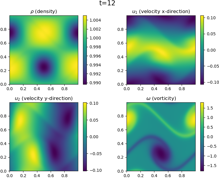
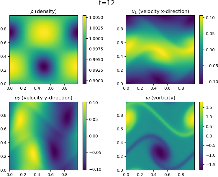
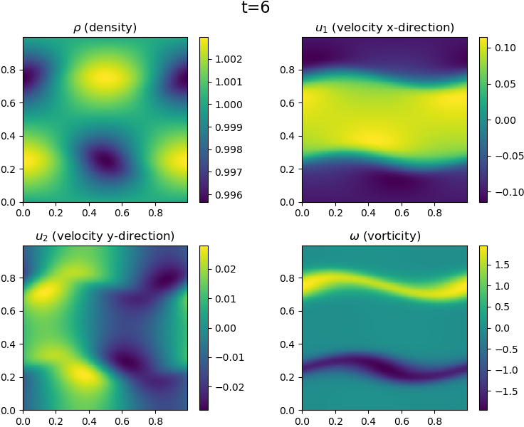
where (x,y)[0,1]2𝑥𝑦superscript012(x,y)\in[0,1]^{2}, v0=0.1subscript𝑣00.1v_{0}=0.1, Δ=1/30Δ130\Delta=1/30, and δ=5103𝛿5superscript103\delta=5\cdot 10^{-3}. Physically the problem models a fluid that moves to the left at the top and bottom of the domain and to the right in the middle of the domain. The small perturbation in the velocity then grows in time and creates a dynamics dominated by vortex structures.

For our dynamical low-rank integrator the moments ρ𝜌\rho, u1subscript𝑢1u_{1}, and u2subscript𝑢2u_{2}, as specified above, are used to initialize a Maxwellian according to equation (1.2) in the domain (v1,v2)[6,6]2subscript𝑣1subscript𝑣2superscript662(v_{1},v_{2})\in[-6,6]^{2}. The Reynolds number Re is prescribed and then ε𝜀\varepsilon is chosen according to ε=v0/Re𝜀subscript𝑣0Re\varepsilon=v_{0}/\text{Re}. That is, we use the flow velocity v0subscript𝑣0v_{0} as the characteristic velocity to define the Reynolds number. Note that this is not entirely consistent with Remark 4.2, where the speed of sound is used instead. However, since the former is the usual choice in the weakly compressible regime, this makes comparison with the literature (e.g. [4, 26, 16]) easier.

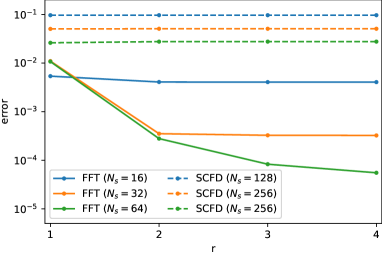
In Figure 1 a comparison at Re=1000Re1000\text{Re}=1000 between a fluid solver based on the MacCormack method [31] and the proposed dynamical low-rank integrator is conducted. We compare density ρ𝜌\rho, velocity u1subscript𝑢1u_{1}, u2subscript𝑢2u_{2}, and vorticity ω=xu2yu1𝜔subscript𝑥subscript𝑢2subscript𝑦subscript𝑢1\omega=\partial_{x}u_{2}-\partial_{y}u_{1} and observe excellent agreement with the fluid solver, as expected. A more quantitative comparison is conducted in Figure 2.

Fluid solver

Refer to caption
Refer to caption

Dynamical low-rank (Fourier spectral method)
Refer to caption
Refer to caption
Figure 1: Numerical simulation of the shear flow (7.1) at time t=6𝑡6t=6 (left) and t=12𝑡12t=12 (right) with Re=103Resuperscript103\text{Re}=10^{3} is shown. The fluid solver (top) uses a MacCormack method, 512512512 grid points in each direction, and is run using a CFL number of 0.9 (Δt1.5103Δ𝑡1.5superscript103\Delta t\approx 1.5\cdot 10^{-3}). The dynamical low-rank integrator (bottom) uses rank r=3𝑟3r=3 and 256256256 grid points in each spatial direction and 323232 grid points in each velocity direction and time step size Δt=2104Δ𝑡2superscript104\Delta t=2\cdot 10^{-4}.
Refer to caption
Figure 2: The error in the moments, i.e. max{ρρref,ρuρuref}subscriptnorm𝜌subscript𝜌refsubscriptnorm𝜌𝑢𝜌subscript𝑢ref\max\{\|\rho-\rho_{\text{ref}}\|_{\infty},\|\rho u-\rho u_{\text{ref}}\|_{\infty}\}, at time t=2𝑡2t=2 is shown as a function of the number of grid points in the x𝑥x and y𝑦y directions (denoted by Nssubscript𝑁𝑠N_{s} in the plot) and the rank r𝑟r. In all cases 323232 grid points in the velocity direction, a time step size of Δt=2105Δ𝑡2superscript105\Delta t=2\cdot 10^{-5}, and Re=1000Re1000\text{Re}=1000 is used. Results are shown both for the SCFD and the FFT based method. We note that the error due to the low-rank approximation is below 102superscript10210^{-2} for r=1𝑟1r=1 and below 104superscript10410^{-4} for r=3𝑟3r=3. The reference solution (ρref,ρuref)subscript𝜌ref𝜌subscript𝑢ref(\rho_{\text{ref}},\rho u_{\text{ref}}) is computed using a MacCormack based fluid solver with 2048×2048204820482048\times 2048 grid points.

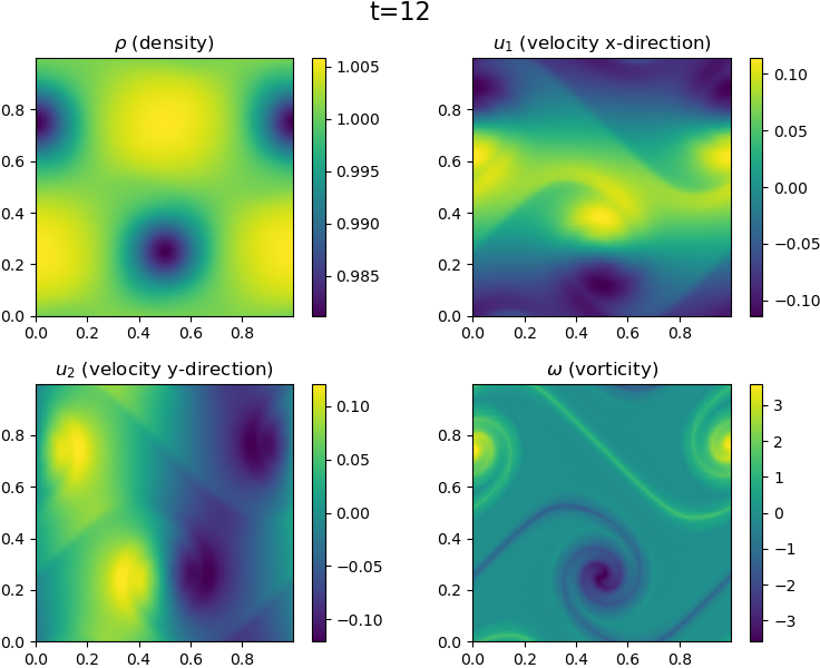
Next, we demonstrate that increasing the Reynolds number (i.e. decreasing ε𝜀\varepsilon) presents no difficulty for our approach. In this case we have to use the SCFD implementation as the Fourier spectral method, as one would expect, produces spurious oscillations and shows stability issues in this regime. The corresponding results are shown in Figure 3 and agree well with the results that have been reported in the literature.

We also remark that choosing a small rank (r=2𝑟2r=2) is sufficient to obtain very accurate results. Let us emphasize that this is in contrast to earlier work [11], where the expansion of the equilibrium mandates that we use a certain rank (at least 666 in 2D and 101010 in 3D). In the method proposed here no assumption on the low-rank structure of the equilibrium needs to be made and thus even a very small rank is sufficient to accurately represent problems which are well described by the fluid limit. We also note that in this limit, as has already been observed in [11], a coarse resolution in the velocity directions is sufficient. This is precisely what we observe in Figure 3.
Refer to caption
Refer to caption
Figure 3: Numerical simulation of the shear flow (7.1) at time t=12𝑡12t=12, Re=105Resuperscript105\text{Re}=10^{5}, and with rank r=2𝑟2r=2 (left) and r=10𝑟10r=10 (right) is shown. The SCFD implementation with 512512512 grid points in each spatial and 323232 grid points in each velocity direction and a time step size of Δt=103Δ𝑡superscript103\Delta t=10^{-3} is used.

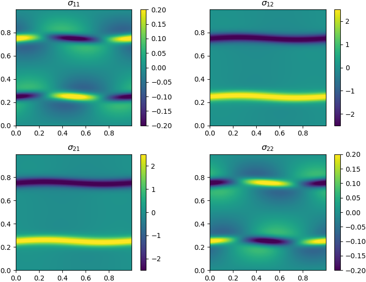
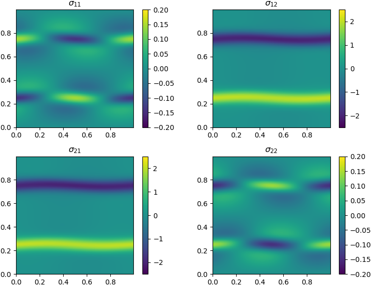
Finally, we investigate the convergence of the stress tensor computed by the kinetic integrator (i.e. the proposed dynamical low-rank algorithm) with the corresponding term in the NS equation. That is, we compare

(1)=1ε(vu)(vu)(fM)𝑑v=1ε[ρ(2π)dv/2ijXiSij(vu)(vu)e|vu|2/2Vj(v)𝑑v+ρId],superscript11𝜀tensor-product𝑣𝑢𝑣𝑢𝑓𝑀differential-d𝑣1𝜀delimited-[]𝜌superscript2𝜋subscript𝑑𝑣2subscript𝑖𝑗subscript𝑋𝑖subscript𝑆𝑖𝑗tensor-product𝑣𝑢𝑣𝑢superscript𝑒superscript𝑣𝑢22subscript𝑉𝑗𝑣differential-d𝑣𝜌Id\mathbb{P}^{(1)}=-\frac{1}{\varepsilon}\int(v-u)\otimes(v-u)(f-M)\,dv=\frac{1}{\varepsilon}\bigg{[}-\frac{\rho}{(2\pi)^{d_{v}/2}}\sum_{ij}X_{i}S_{ij}\int(v-u)\otimes(v-u)e^{-|v-u|^{2}/2}V_{j}(v)\,dv+\rho\text{Id}\bigg{]}, (7.2)

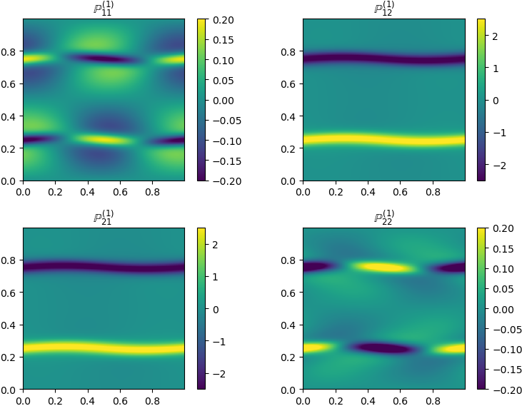
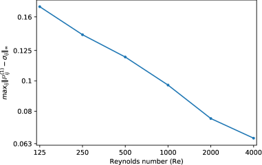
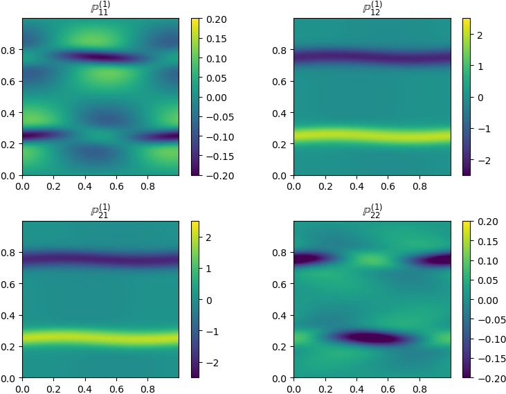
obtained by the dynamical low-rank integrator, with σ(u)𝜎𝑢\sigma(u) (defined in (2.13)) obtained from the fluid solver (here dv=2subscript𝑑𝑣2d_{v}=2). To evaluate equation (7.2), without incurring the cost of forming the entire density function, we once again write the integral as a convolution (as described in Section 4.1). We know from theory that (1)superscript1\mathbb{P}^{(1)} converges to σ(u)𝜎𝑢\sigma(u) as ε0𝜀0\varepsilon\to 0 (see Section 2). This is also observed in the numerical results shown in Figure 4 and Figure 5. In Figure 5 we have plotted the difference between these two quantities as a function of the Reynolds number.
Re=500𝑅𝑒500Re=500

Refer to caption
Refer to caption

Re=4000𝑅𝑒4000Re=4000

Refer to caption
Refer to caption
Figure 4: Comparison of σ(u)𝜎𝑢\sigma(u), computed with the MacCormack based fluid solver, with the stress tensor (1)superscript1\mathbb{P}^{(1)}, computed with the dynamical low-rank approximation, for Re=500𝑅𝑒500Re=500 and Re=4000𝑅𝑒4000Re=4000. All simulations are conducted with rank r=5𝑟5r=5, 512512512 grid points in each spatial direction, 646464 grid points in each velocity direction, and a time step size of Δt=5105Δ𝑡5superscript105\Delta t=5\cdot 10^{-5}.
Refer to caption
Figure 5: Difference between σ(u)𝜎𝑢\sigma(u), computed with the fluid solver, and the stress tensor (1)superscript1\mathbb{P}^{(1)}, computed with the dynamical low-rank approximation, in the maximum norm and as a function of the Reynolds number is shown. All simulations are conducted until t=2𝑡2t=2 and with r=5𝑟5r=5, 512512512 grid points in each spatial direction, 646464 grid points in each velocity direction, and a time step size of Δt=5105Δ𝑡5superscript105\Delta t=5\cdot 10^{-5}.

7.2 Explosion

In this section we consider an initial overpressure in a small region that expands and results in a propagating shock wave, i.e. an explosion. We will use the following initial value

ρ(0,x,y)={1,x2+y2R2,110,otherwise,u1(0,x,y)=0,u2(0,x,y)=0,\displaystyle\begin{split}\rho(0,x,y)&=\begin{cases}1,&x^{2}+y^{2}\leq R^{2},\\ \tfrac{1}{10},&\text{otherwise},\end{cases}\\ u_{1}(0,x,y)&=0,\qquad u_{2}(0,x,y)=0,\end{split} (7.3)

with (x,y)[1.5,1.5]2𝑥𝑦superscript1.51.52(x,y)\in[-1.5,1.5]^{2} and R=102𝑅superscript102R=10^{-2}. As before, the specified moments are used to initialize a Maxwellian according to equation (1.2) in the domain (v1,v2)[6,6]2subscript𝑣1subscript𝑣2superscript662(v_{1},v_{2})\in[-6,6]^{2}. This is a good example to demonstrate that our scheme is able to resolve sharp gradients/shocks in a compressible flow.

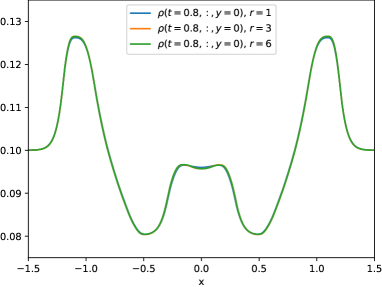
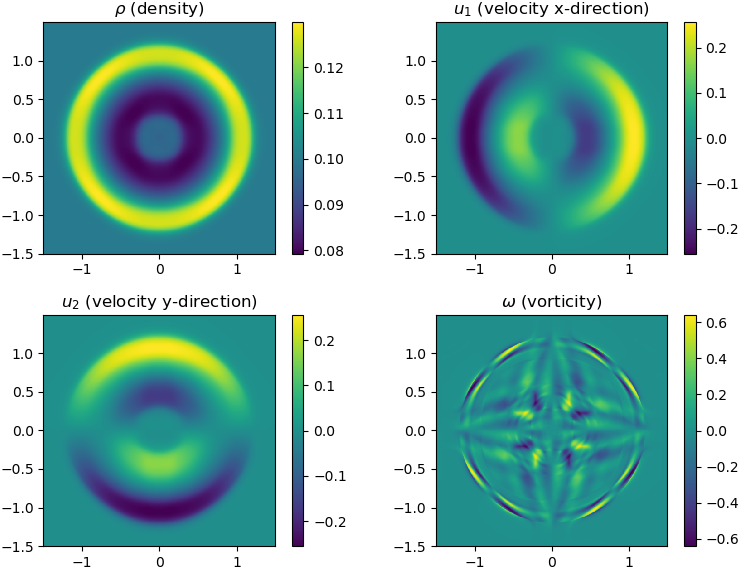
The numerical results are shown in Figure 6. We clearly observe the shock front that radially propagates outward starting from the center. Let us also emphasize that, for ε=105𝜀superscript105\varepsilon=10^{-5}, a small rank is sufficient to resolve the dynamics; in fact, starting from r=3𝑟3r=3 the solutions produced by the low-rank integrator are indistinguishable in the plot.
Refer to caption
Refer to caption
Figure 6: Numerical simulation of the explosion (7.3) at time t=0.8𝑡0.8t=0.8, ε=105𝜀superscript105\varepsilon=10^{-5}, and with rank r=6𝑟6r=6 is shown on the left. The SCFD implementation with 512512512 grid points in each spatial and 323232 grid points in each velocity direction and a time step size of Δt=5105Δ𝑡5superscript105\Delta t=5\cdot 10^{-5} is used. On the right a slice through the solution, at y=0𝑦0y=0, is shown for r=1𝑟1r=1, r=3𝑟3r=3, and r=6𝑟6r=6.

7.3 Beam relaxation

In this section we consider a fully kinetic problem, i.e. a problem where the dynamics is not well represented by the fluid limit. A beam with a constant velocity and Maxwellian distribution propagates into a stationary gas. The initial value is given by [8]

f(0,x,y,v,w)=12π(e(v2+w2)/2+nbe((vvb)2+(wwb)2)/(2Tb)),𝑓0𝑥𝑦𝑣𝑤12𝜋superscript𝑒superscript𝑣2superscript𝑤22subscript𝑛𝑏superscriptesuperscript𝑣subscript𝑣𝑏2superscript𝑤subscript𝑤𝑏22subscript𝑇𝑏f(0,x,y,v,w)=\frac{1}{\sqrt{2\pi}}\left(e^{-(v^{2}+w^{2})/2}+n_{b}\mathrm{e}^{-((v-v_{b})^{2}+(w-w_{b})^{2})/(2T_{b})}\right), (7.4)

where (x,y,v,w)[0,1]2×[8,8]2𝑥𝑦𝑣𝑤superscript012superscript882(x,y,v,w)\in[0,1]^{2}\times[-8,8]^{2}, nb=103subscript𝑛𝑏superscript103n_{b}=10^{-3}, vb=4subscript𝑣𝑏4v_{b}=4 , wb=2subscript𝑤𝑏2w_{b}=2, Tb=0.1subscript𝑇𝑏0.1T_{b}=0.1. This is a rank 1 initial value that in our framework, i.e. with f=Mg𝑓𝑀𝑔f=Mg, is represented as follows

ρ=1,u1=u2=0,formulae-sequence𝜌1subscript𝑢1subscript𝑢20\rho=1,\qquad u_{1}=u_{2}=0,

and

g=1+nbe((vvb)2+(wwb)2)/(2Tb)+(v2+w2)/2.𝑔1subscript𝑛𝑏superscriptesuperscript𝑣subscript𝑣𝑏2superscript𝑤subscript𝑤𝑏22subscript𝑇𝑏superscript𝑣2superscript𝑤22g=1+n_{b}\mathrm{e}^{-((v-v_{b})^{2}+(w-w_{b})^{2})/(2T_{b})+(v^{2}+w^{2})/2}.

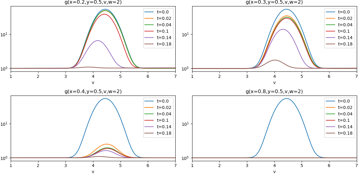
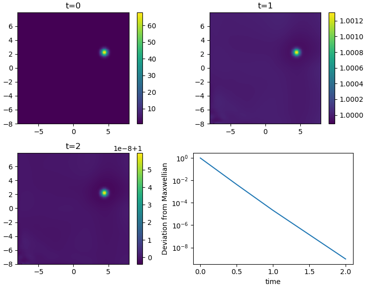
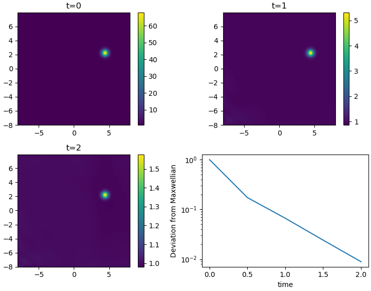
The expected behavior is that the perturbation (the beam) in velocity space diminishes over time according to exp(t/ε)𝑡𝜀\exp(-t/\varepsilon). That is, the collisions thermalize the beam until it is indistinguishable from the background gas. This problem has been considered in the context of hybrid kinetic-fluid models in [8]. The hybrid method proposed there, which treats fast particles kinetically and the slow particles by a fluid model, has difficulties in capturing the physical behavior.

The numerical results using the low-rank integrator are presented in Figure 7. Note that because the initial value is homogeneous in the x𝑥x directions we can use a relatively coarse resolution in space. For ε=0.1𝜀0.1\varepsilon=0.1/ε=0.5𝜀0.5\varepsilon=0.5 the deviation from equilibrium reduces by approximately 109superscript10910^{-9}/102superscript10210^{-2}, which clearly demonstrates that the low-rank algorithm accurately reproduce the expected decay rates.
Refer to caption
Refer to caption
Figure 7: We plot g(0,0,:,:)𝑔00::g(0,0,:,:) for the beam relaxation problem (7.4) at time t=0𝑡0t=0, t=1𝑡1t=1, and t=2𝑡2t=2 and for ε=0.1𝜀0.1\varepsilon=0.1 (left) and ε=0.5𝜀0.5\varepsilon=0.5 (right). The SCFD implementation with r=10𝑟10r=10, 323232 grid points in each spatial and 256256256 grid points in each velocity direction, and a time step size of Δt=104Δ𝑡superscript104\Delta t=10^{-4} is used. On the bottom right the maximal deviation from equilibrium, i.e. the deviation in the maximum norm (normalized to the initial value), is shown as a function of time.

7.4 Beam relaxation with spatially varying ε𝜀\varepsilon

One interesting application of the proposed dynamical low-rank integrator is in applications where the Knudsen number ε𝜀\varepsilon varies over several orders of magnitude (see the discussion on hybrid kinetic/fluid schemes in the Introduction). We explore this here in the context of the beam relaxation problem introduced in the previous section with a spatially varying ε𝜀\varepsilon given by

ε(x,y)=ε0+tanh(111x)+tanh(1+11x),𝜀𝑥𝑦subscript𝜀0111𝑥111𝑥\varepsilon(x,y)=\varepsilon_{0}+\tanh(1-11x)+\tanh(1+11x), (7.5)

with ε0=104subscript𝜀0superscript104\varepsilon_{0}=10^{-4} in the spatial domain (x,y)[1,1]×[0,1]𝑥𝑦1101(x,y)\in[-1,1]\times[0,1]. Thus, we have ε1𝜀1\varepsilon\approx 1 in the middle of the domain (kinetic regime) and ε104𝜀superscript104\varepsilon\approx 10^{-4} (fluid regime) as we get closer to the boundary.

The numerical results obtained are shown in Figure 8. We investigate here the deviation from equilibrium as a function of velocity. We observe that the thermalization proceeds with different speeds depending on the value of ε𝜀\varepsilon on that part of the domain, as we would expected. We have also compared numerical simulations obtained with different ranks. For r=3𝑟3r=3 a significant deviation from the reference solution (computed with r=60𝑟60r=60) can be observed. However, starting with rank r=10𝑟10r=10 the low-rank error is small and we observe excellent agreement with the reference solution.

Dynamical low-rank with r=3𝑟3r=3
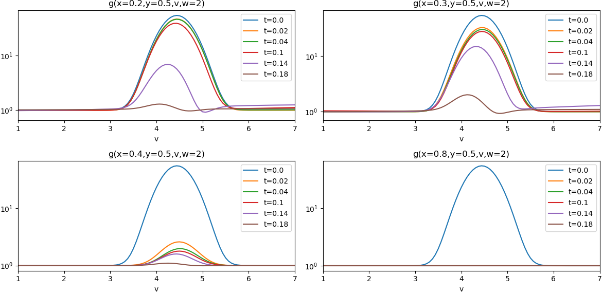
Refer to caption

Dynamical low-rank with r=10𝑟10r=10

Refer to caption

Dynamical low-rank with r=60𝑟60r=60

Refer to caption
Figure 8: We plot slices through g𝑔g corresponding to x=0.2,0.3,0,4,0.8𝑥0.20.3040.8x=0.2,0.3,0,4,0.8 and y=0.5𝑦0.5y=0.5, w=2𝑤2w=2 for the beam relaxation problem (7.4) with spatially varying ε𝜀\varepsilon given by equation (7.5). In all directions (both space and velocity) 256256256 grid points are employed and the SCFD scheme (with δxsubscript𝛿𝑥\delta_{x} in equation (5.1) discretized by upwinding) and a time step size of Δt=5105Δ𝑡5superscript105\Delta t=5\cdot 10^{-5} is used in all simulations.

References

  • [1] P. Andries, P. Le Tallec, J.-P. Perlat, and B. Perthame. The Gaussian-BGK model of Boltzmann equation with small Prandtl number. Eur. J. Mech. B/Fluids, 19:813–830, 2000.
  • [2] A. Arnold and T. Jahnke. On the approximation of high-dimensional differential equations in the hierarchical Tucker format. BIT Numerical Mathematics, 54(2):305–341, 2014.
  • [3] C. Bardos, F. Golse, and D. Levermore. Fluid dynamic limits of kinetic equations. I. Formal derivations. J. Stat. Phys., 63:323–344, 1991.
  • [4] J.B. Bell, P. Colella, and H.M Glaz. A second-order projection method for the incompressible Navier-Stokes equations. J. Comput. Phys., 85(2):257–283, 1989.
  • [5] P. Bhatnagar, E. Gross, and M. Krook. A model for collision processes in gases. I. Small amplitude processes in charged and neutral one-component systems. Phys. Rev., 94:511–525, 1954.
  • [6] C. Cercignani. The Boltzmann Equation and Its Applications. Springer-Verlag, New York, 1988.
  • [7] D. Conte and C. Lubich. An error analysis of the multi-configuration time-dependent Hartree method of quantum dynamics. ESAIM Math. Model. Numer. Anal., 44(4):759–780, 2010.
  • [8] N. Crouseilles, P. Degond, and M. Lemou. A hybrid kinetic–fluid model for solving the Vlasov–BGK equation. J. Comput. Phys., 203(2):572–601, 2005.
  • [9] G. Dimarco and L. Pareschi. Numerical methods for kinetic equations. Acta Numer., 23:369–520, 2014.
  • [10] Z. Ding, L. Einkemmer, and Q. Li. Error analysis of an asymptotic preserving dynamical low-rank integrator for the multi-scale radiative transfer equation. arXiv:1907.04247, 2019.
  • [11] L. Einkemmer. A low-rank algorithm for weakly compressible flow. SIAM J. Sci. Comput., 41(5):A2795–A2814, 2019.
  • [12] L. Einkemmer, J. Hu, and Y. Wang. An asymptotic-preserving dynamical low-rank method for the multi-scale multi-dimensional linear transport equation. arXiv:2005.06571, 2020.
  • [13] L. Einkemmer and C. Lubich. A low-rank projector-splitting integrator for the Vlasov–Poisson equation. SIAM J. Sci. Comput., 40:B1330–B1360, 2018.
  • [14] L. Einkemmer and C. Lubich. A quasi-conservative dynamical low-rank algorithm for the Vlasov equation. SIAM J. Sci. Comput., 41(5):B1061–B1081, 2019.
  • [15] L. Einkemmer, A. Ostermann, and C. Piazzola. A low-rank projector-splitting integrator for the Vlasov–Maxwell equations with divergence correction. J. Comput. Phys., 403:109063, 2020.
  • [16] L. Einkemmer and M. Wiesenberger. A conservative discontinuous Galerkin scheme for the 2D incompressible Navier–Stokes equations. Comput. Phys. Commun., 185(11):2865–2873, 2014.
  • [17] F. Filbet and T. Rey. A Hierarchy of Hybrid Numerical Methods for Multiscale Kinetic Equations. SIAM J. Sci. Comput., 37(3):A1218–A1247, 2015.
  • [18] J. Hu, S. Jin, and Q. Li. Asymptotic-preserving schemes for multiscale hyperbolic and kinetic equations. In R. Abgrall and C.-W. Shu, editors, Handbook of Numerical Methods for Hyperbolic Problems: Applied and Modern Issues, chapter 5, pages 103–129. North-Holland, 2017.
  • [19] G.-S. Jiang and E. Tadmor. Nonoscillatory central schemes for multidimensional hyperbolic conservation laws. SIAM J. Sci. Comput., 19(6):1892–1917, 1998.
  • [20] E. Kieri, C. Lubich, and H. Walach. Discretized dynamical low-rank approximation in the presence of small singular values. SIAM J. Numer. Anal., 54(2):1020–1038, 2016.
  • [21] O. Koch and C. Lubich. Dynamical low-rank approximation. SIAM J. Matrix Anal. Appl., 29(2):434–454, 2007.
  • [22] O. Koch and C. Lubich. Dynamical tensor approximation. SIAM J. Matrix Anal. Appl., 31(5):2360–2375, 2010.
  • [23] K. Kormann. A semi-Lagrangian Vlasov solver in tensor train format. SIAM J. Sci. Comput., 37:613–632, 2015.
  • [24] K. Kormann and E. Sonnendrücker. Sparse grids for the Vlasov–Poisson equation. In Sparse Grids and Applications, pages 163–190. Springer, 2016.
  • [25] R.J. LeVeque. Numerical methods for conservation laws. Springer, 1992.
  • [26] J. Liu and C. Shu. A high-order discontinuous Galerkin method for 2D incompressible flows. J. Comput. Phys., 160(2):577–596, 2000.
  • [27] C. Lubich. From quantum to classical molecular dynamics: reduced models and numerical analysis. European Mathematical Society, Zürich, 2008.
  • [28] C. Lubich. Time integration in the multiconfiguration time-dependent Hartree method of molecular quantum dynamics. Appl. Math. Res. Express. AMRX, 2015:311–328, 2015.
  • [29] C. Lubich and I.V. Oseledets. A projector-splitting integrator for dynamical low-rank approximation. BIT Numer. Math., 54(1):171–188, 2014.
  • [30] C. Lubich, T. Rohwedder, R. Schneider, and B. Vandereycken. Dynamical approximation by hierarchical Tucker and tensor-train tensors. SIAM J. Matrix Anal. Appl., 34(2):470–494, 2013.
  • [31] R.W. MacCormack. The effect of viscosity in hypervelocity impact cratering. J. Spacecr. Rockets, 40(5):757–763, 2003.
  • [32] H.-D. Meyer, F. Gatti, and G. A. Worth. Multidimensional quantum dynamics. John Wiley & Sons, 2009.
  • [33] H.-D. Meyer, U. Manthe, and L. S. Cederbaum. The multi-configurational time-dependent Hartree approach. Chem. Phys. Letters, 165(1):73–78, 1990.
  • [34] H. Nessyahu and E. Tadmor. Non-oscillatory central differencing for hyperbolic conservation laws. J. Comput. Phys., 87(2):408–463, 1990.
  • [35] Z. Peng, R. McClarren, and M. Frank. A low-rank method for two-dimensional time-dependent radiation transport calculations. arXiv:1912.07522, 2019.
  • [36] E. Shakhov. Generalization of the Krook kinetic relaxation equation. Fluid Dynamics, 3:95–96, 1968.
  • [37] H. Struchtrup. Macroscopic Transport Equations for Rarefied Gas Flows. Springer, 2005.
  • [38] J. Vencels, G.L. Delzanno, A. Johnson, I.B. Peng, E. Laure, and S. Markidis. Spectral Solver for Multi-scale Plasma Physics Simulations with Dynamically Adaptive Number of Moments. Procedia Comput. Sci., 51:1148–1157, 2015.