Diffuseness parameter as a bottleneck for accurate half-life calculations

Abstract

An investigation of the calculated $\alpha$ decay half-lives of super heavy nuclei (SHN) reveals that the diffuseness parameter is a great bottleneck for achieving accurate results and predictions. In particular, when universal proximity function is adopted for nuclear potential, half-life is found to vary significantly and nonlinearly as a function of diffuseness parameter. To overcome this limiting hurdle, a new semiempirical formula for diffuseness that is dependent on charge and neutron numbers is proposed in this work. With the model at hand, half-lives of 218 SHN are computed, for 68 of which there exists available experimental data and 150 of which are predicted. The calculations of half-lives for 68 SHN are compared against experimental data and the calculated data obtained by using deformed Woods-Saxon, deformed Coulomb potentials model, and six semiempirical formulas. The predictions of 150 SHN are compared against the predictions of seven of the current best semiempirical formulas. Calculations of the present study are in good agreement with the experimental half-lives outperforming all but ImSahu semiempirical formula. Moreover, the predictions of our model are consistent with predictions of the semiempirical formulas. We strongly conclude that more attention should be directed toward obtaining accurate diffuseness parameter values for using it in nuclear calculations.

I Introduction

Currently, within the theoretical framework of nuclear physics, especially in $\alpha$ decay of super heavy nuclei (SHN), there are points of intersection and divergence between different models used in calculations. Particularly, points of disagreement abound, including the particular functional form of nuclear interaction between $\alpha$/cluster and the daughter nuclei, be it given by Woods-Saxon (WS) potential [1], double folding model (DFM) [2, 3], liquid drop model (LDM) [4], universal proximity potential [5, 6] and et cetera. Another point of disagreement stems from two competing proposals for $\alpha$ decay. The first–often dubbed cluster-like theory– assigns a preformation factor $P_{o}$ for every parent nuclei, while the second fission-like model asserts that $P_{o}=1$ for all nuclei [7]. On the other hand, the diffuseness parameter $a$ is one of the parameters with universal presence in all models regardless of the particular nuclear potential under study. Although ubiquitous, little attention is paid to the parameter which is often set constant for all nuclei [1, 8, 9, 10, 11]. More recently, Dehghani et al. investigated the role diffuseness parameter plays when deformed Woods-Saxon potential is adopted for nuclear interaction between $\alpha$ and daughter nuclei. Some interesting conclusions were reached of which we list the chief ones [12]:

1. The logarithm of half-life $\log_{10}T_{1/2}$ decreases linearly with increasing diffuseness parameter. For instance, a variation of 0.4 fm of $a$ can induce a change in the logarithm of half-life by 2 (i.e., half-life changes by two orders of magnitude).

2. For a given nucleus, a systematic search was carried out in search for the best $a$ value that matches the experimental half-life for that particular nucleus. This process was applied on 68 SHN and diffuseness parameter for 68 SHN was extracted out of experimental data of half-lives.

3. Adopting a constant $a=0.54$ fm for all nuclei was found to be optimal in the sense of minimizing the root-mean-square (rms) error of the logarithm of half-lives. The rms error came out to be 0.787, implying that on average, adopting $a=0.54$ fm will induce an error of 0.787 for the logarithm of half-life.

Our work extends and generalizes these results by investigating the effect of diffuseness parameter when universal proximity potential is adopted for nuclear interaction between $\alpha$ and daughter nuclei. The outline of this paper is as follows: in Sec. II, we outline the theoretical framework that we will be working with regarding calculations of half-lives. In Sec. III, the relation between diffuseness and half-life is probed when proximity potential is adopted and results are compared with the case of deformed WS, deformed Coulomb potentials. In Sec. IV, we investigate the relation between diffuseness parameter on one hand and charge, neutron and mass numbers on the other, and we propose a new semiempirical formula for diffuseness as a function of charge and neutron numbers. In Sec. V, calculations and predictions of 218 SHN are made; calculations for 68 SHN will be carried out using proximity potential with variable effective diffuseness and compared with calculations of deformed WS, deformed Coulomb potentials in which diffuseness parameter is set to $a=0.54$ fm. Moreover, our calculations will be compared with six popular semiempirical formulas for half-lives. The viability of the new formula for diffuseness is tested by predicting the half-lives of 150 SHN and comparing the results with seven of the current best semiempirical formulas. We conclude the last section by discussing the most important highlights, results, and potential research directions in the future.

II Theoretical framework

Generally, the effective potential for $\alpha$ decay can be broken into three contributions, namely nuclear, Coulomb, and angular contributions

$$V_{\text{eff}}(r)=V_{N}(r)+V_{C}(r)+V_{l}(r)$$ (1)

where $r$ is the separation distance between the center of the daughter and $\alpha$ nuclei. For our particular potential, we assume spherical symmetry and ignore deformation effects, i.e., we consider the potential to assume radial dependence only, with the quadrupole and hexadecapole deformation parameters $\beta_{2}$ and $\beta_{4}$ set to zero. Moreover, we shall consider cases in which there’s no total angular momentum carried by the $\alpha$-daughter system and hence $V_{l}(r)$ is subsequently ignored. Regarding the nuclear term $V_{N}(r)$, we adopt the universal proximity potential previously proposed by Zhang et al. [5]:

$$V_{N}(s_{0})=4\pi b_{\text{eff}}\macc@depth\char 1\relax\frozen@everymath{\macc@group}\macc@set@skewchar\macc@nested@a 111{R}\gamma\phi(s_{0})$$ (2)

$$\phi(s_{0})=\dfrac{p_{1}}{1+\exp\Big{(}\dfrac{s_{0}+p_{2}}{p_{3}}\Big{)}}$$ (3)

In two parameter Fermi distribution (2pF) of nuclear matter, $b_{\text{eff}}$ and the effective diffuseness $a_{\text{eff}}$ of the proximity potential are related as

$$b_{\text{eff}}=\dfrac{\pi}{\sqrt{3}}a_{\text{eff}}$$ (4)

The effective diffuseness is a function of both the nuclear surface diffuseness of the daughter and $\alpha$ nuclei. Following previous works [5, 13], we posit the ansatz that $a_{\text{eff}}$ is the average of the two, i.e., $a_{\text{eff}}=(a_{\alpha}+a_{d})/2$ with $a_{\alpha}=0.3238$ fm and $a_{d}$ refers to the nuclear surface diffuseness of the daughter. We shall explain and show hereafter that adopting a constant $a_{\text{eff}}$ for all nuclei leads to unacceptable errors, especially for the proximity potential and for systems in which we expect that $a_{\text{eff}}\geq 0.5$ fm (or equivalently $b_{\text{eff}}\geq 0.9$ fm). $\gamma$ is given by

$$\gamma=0.9517\Big{[}1-1.7826\Big{(}\dfrac{N-Z}{A}\Big{)}^{2}\Big{]}\,$\mathrm{MeV}\text{\,}{\mathrm{fm}}^{-2}$$$ (5)

$\macc@depth\char 1\relax\frozen@everymath{\macc@group}\macc@set@skewchar\macc@nested@a 111{R}=R_{\alpha}R_{d}/(R_{\alpha}+R_{d})$ is the reduced radius of the $\alpha$-daughter system where the radius of each nucleus in terms of its mass number is given by

$$R=1.28A^{1/3}+0.8A^{-1/3}-0.76$$ (6)

$\phi(s_{0})$ is the universal function that quantifies the nuclear interaction between $\alpha$ and the daughter in terms of the reduced separation distance $s_{0}$

$$s_{0}=\dfrac{r-R_{\alpha}-R_{d}}{b_{\text{eff}}}$$ (7)

In particular, this equation holds in the regime $s_{0}>-1$. The constants $p_{1},p_{2}$ and $p_{3}$ appearing in Eq. (3) are given by -7.65, 1.02 and 0.89 respectively. Moving on, the Coulomb term $V_{C}(r)$ is given by

$$V_{C}(r)=Z_{\alpha}Z_{d}e^{2}\left\{\begin{array}[]{ll}\dfrac{1}{r}&r\geq R_{C}\\ \dfrac{1}{2R_{C}}\Big{[}3-\Big{(}\dfrac{r}{R_{C}}\Big{)}^{2}\Big{]}&r<R_{C}\end{array}\right.$$ (8)

where $Z_{\alpha}$ and $Z_{d}$ are the $\alpha$ and daughter charge numbers and $R_{C}=R_{\alpha}+R_{d}$. In the context of WKB approximation, the half-life is given by

$$T_{1/2}=\dfrac{\pi\hbar\ln 2}{P_{o}E_{\nu}}\Big{(}1+\exp(K)\Big{)}$$ (9)

where $P_{o},E_{\nu}$ and $K$ are the preformation factor, zero-point vibration energy and action integral respectively. The action integral is given by

$$K=\dfrac{2}{\hbar}\int_{r_{1}}^{r_{2}}\sqrt{2\mu(V_{\text{eff}}(r)-Q_{\alpha})}dr$$ (10)

where $Q_{\alpha},\mu,r_{1}$, and $r_{2}$ are the decay energy, reduced mass, and first and second turning points, respectively. We shall describe $E_{\nu}$ classically, since it was previously found [7] that classical and quantum mechanical (e.g., modified harmonic oscillator) approaches yield not too different results, hence

$$E_{\nu}=\dfrac{\hbar\omega}{2}=\dfrac{\hbar\pi}{2R_{p}}\sqrt{\dfrac{2E_{\alpha}}{m_{\alpha}}}$$ (11)

where $R_{p},E_{\alpha}$ and $m_{\alpha}$ are the parent radius, kinetic energy of $\alpha$ nuclei and its mass respectively. The decay energy of the system and the kinetic energy of $\alpha$ nuclei are related by the recoil of the daughter and electron shielding, or in other words [14],

$$E_{\alpha}=\dfrac{A_{d}}{A_{p}}Q_{\alpha}-\Big{(}6.53Z_{d}^{7/5}-8Z_{d}^{2/5}\Big{)}\cdot 10^{-5}\,$\mathrm{MeV}$$$ (12)

where $A_{d}$ and $A_{p}$ are the mass numbers of the daughter and the parent nuclei respectively. Finally, for the preformation factor, we adopt [15]

$$\log_{10}P_{o}=a+b(Z-Z_{1})(Z_{2}-Z_{1})+c(N-N_{1})(N_{2}-N)\\ +dA+e(Z-Z_{1})(N-N_{1})$$ (13)

where $a,b,c,d$ and $e$ are given by 34.90593, 0.003011, 0.003717, -0.151216 and 0.006681 respectively. For $82\leq Z\leq 126$ and $152\leq N\leq 184$, which is the scope of the present paper, the magic numbers $Z_{1},Z_{2},N_{1}$ and $N_{2}$ are given by 82, 126, 152 and 184 respectively.

III Diffuseness and half-life for proximity potential

A priori, one should not expect the effective diffuseness parameter $a_{\text{eff}}$ for the proximity potential and the diffuseness parameter for WS potential $a_{\text{\tiny WS}}$ to be equal or even play the same logical roles; this is owing to the different functional forms of the two potentials. To be more precise, consider the undeformed WS potential [1]

$$V_{\text{\tiny WS}}(r)=\dfrac{-V_{0}}{1+\exp\Big{(}\dfrac{r-R_{0}}{a_{\text{\tiny WS}}}\Big{)}}$$ (14)

where $V_{0}$ is the depth of the potential well and $R_{0}$ is the half radius at which $V(R_{0})=-V_{0}/2$. One can easily see that letting $a_{\text{\tiny WS}}\rightarrow\infty$ leads to $V_{\text{\tiny WS}}(r)\rightarrow-V_{0}/2$ for all $r$, while $a_{\text{\tiny WS}}\rightarrow 0$ leads to $V_{\text{\tiny WS}}(r)\rightarrow-V_{0}$ for $r\leq R_{0}$. In other words, smaller $a_{\text{\tiny WS}}$ leads to a deeper potential well (and vice versa) with the depth of the potential varying from $-V_{0}$ to $-V_{0}/2$.

Regarding the proximity potential, however, from Eqs. (2), (3) and (7), we see that $a_{\text{eff}}\rightarrow\infty$ leads to $V_{N}(r)\rightarrow-\infty$ for all $r$, while $a_{\text{eff}}\rightarrow 0$ leads to $V_{N}(r)\rightarrow 0$ for all $r$; that is, greater $a_{\text{eff}}$ leads to a deeper potential well (unlike the WS case) and vice versa, with the depth of the potential varying from $-\infty$ to 0.

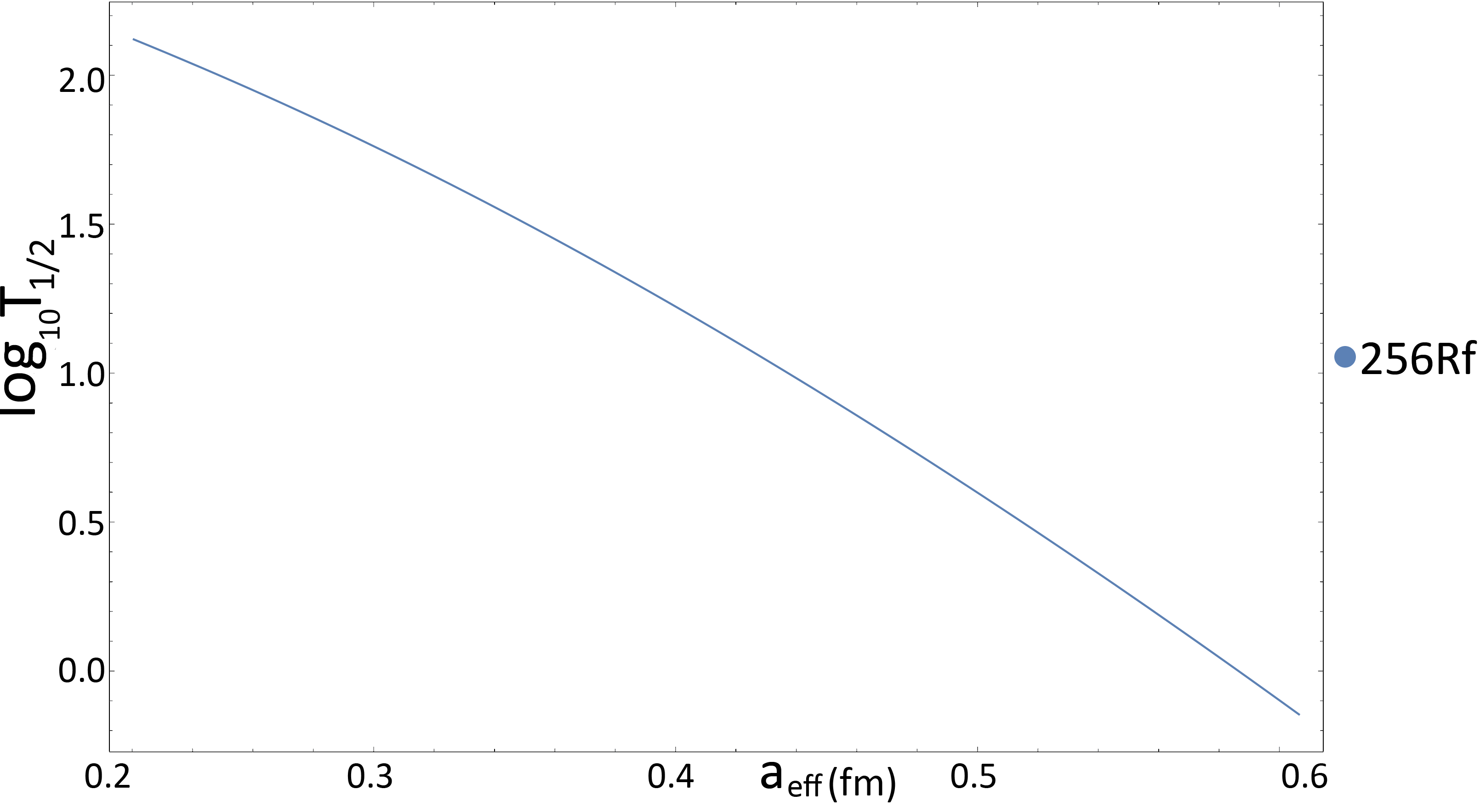
Figure 1: $\log_{10}T_{1/2}$ vs. $a_{\text{eff}}$ (fm) for 256Rf.

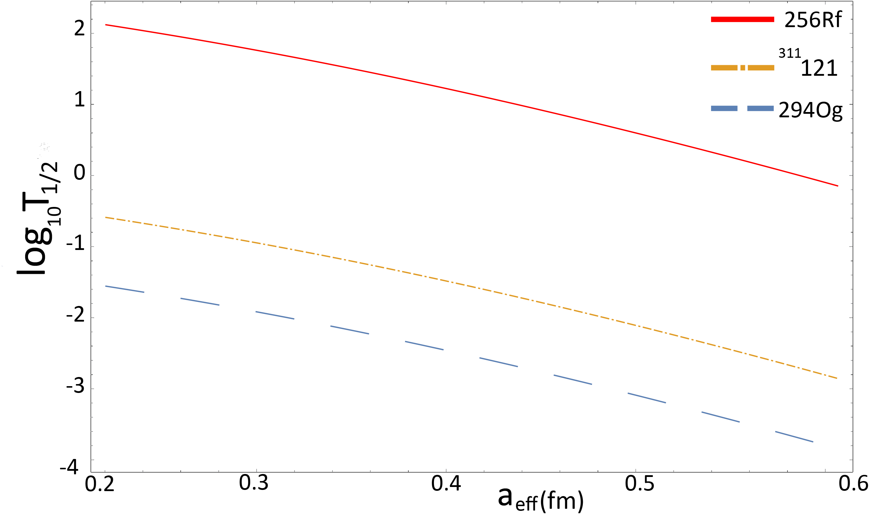
Figure 2: $\log_{10}T_{1/2}$ vs. $a_{\text{eff}}$ (fm) for three different SHN.

This is the motivation behind the current investigation. In this section, we shall study how half-lives of nuclei vary with $a_{\text{eff}}$. Simulation results displayed in Fig. 1 and 2 show variation of the logarithm of half-life with $a_{\text{eff}}$ as it’s varied from 0.22 to 0.61 fm. Simulation results are interesting insofar that they intersect and diverge from the previous work which investigated the role of diffuseness [12]. Both results confirm the physical intuition that half-life is a monotonically decreasing function of diffuseness parameter; this is to be expected since increasing $a_{\text{eff}}$ increases the range of nuclear interaction $R$ which dominates the Coulomb force, leading to a decreased potential height and hence increased penetrability of the barrier and a decrease in half-life. More interesting perhaps is the different behavior exhibited by half-life when proximity potential is adopted instead of deformed WS, deformed Coulomb potentials as in the previous study [12]. Unlike the WS case–in which half-life varies linearly with diffuseness parameter– the half-life here is a non-linear convex function of the effective diffuseness $a_{\text{eff}}$. In Fig. 1, we can see that variation of diffuseness from 0.22 to 0.61 fm leads to change in the logarithm of half-life from 2.1 to -0.1– two orders of magnitude change in the half-life (equivalently, $b_{\text{eff}}$ was varied from 0.4 to 1.1 fm). In addition to the significant change in half-life with small variations in diffuseness, the non-linear convex behavior implies that for systems with $a_{\text{eff}}>0.5$ fm, approximating diffuseness as 0.54 fm is problematic since half-life varies even stronger with diffuseness compared to the region $a_{\text{eff}}<0.5$ fm; to illustrate with an example, consider the case of 256Rf shown in Fig. 1, varying $a_{\text{eff}}$ by 0.1 fm from 0.22 to 0.32 fm induces a change of 0.457 in the logarithm of half-life, while varying $a_{\text{eff}}$ from 0.5 to 0.6 fm leads to a change in the half-life by 0.69. These two aforementioned facts– significant change with slight diffuseness variation and convexity/non-linearity– deem common approximations [16, 5, 17, 18, 19, 20] such as $b_{\text{eff}}=0.99-1$ fm unacceptable since they’re bound to produce large errors. Fig. 2 helps to illustrate the universality of this behavior irrespective of the SHN under study.

IV New semiempirical formula for $a_{\text{eff}}$

In their work, Dehghani et al. considered deformed WS, deformed Coulomb potentials and investigated 68 SHN in the region $104\leq Z\leq 118$ [12]. For every nucleus, a systematic search was carried out looking for the optimal $a_{\text{\tiny WS}}$ value that matches the experimental half-life for that particular nucleus. The result of their work is plotted in Fig. 3 in which diffuseness $a_{\text{\tiny WS}}$ is plotted against $Z,N$, and $A$. We see that $a_{\text{\tiny WS}}$ can be as large as 0.86 fm for the particular nucleus under study. Moreover, the general trend is an increase of $a_{\text{\tiny WS}}$ when $Z$ and $N$ (or equivalently $A$) is increased although this is not a strict rule. To map $a_{\text{\tiny WS}}$ into $a_{\text{eff}}$, we posit the ansatz that $a_{\text{eff}}=(a_{\alpha}+a_{\text{\tiny WS}})/2$; the reasonableness and viability of this assumption will be addressed by the results in the following section. By mapping $a_{\text{\tiny WS}}$ into $a_{\text{eff}}$, we get the plot in Fig. 4 for effective diffuseness vs. $Z,N$, and $A$. Next, we tried fitting both $a_{\text{\tiny WS}}$ and $a_{\text{eff}}$ vs. $Z$ and $N$. Various fitting schemes including linear and non-linear ones were considered and tried. We list the two main results of these attempts:

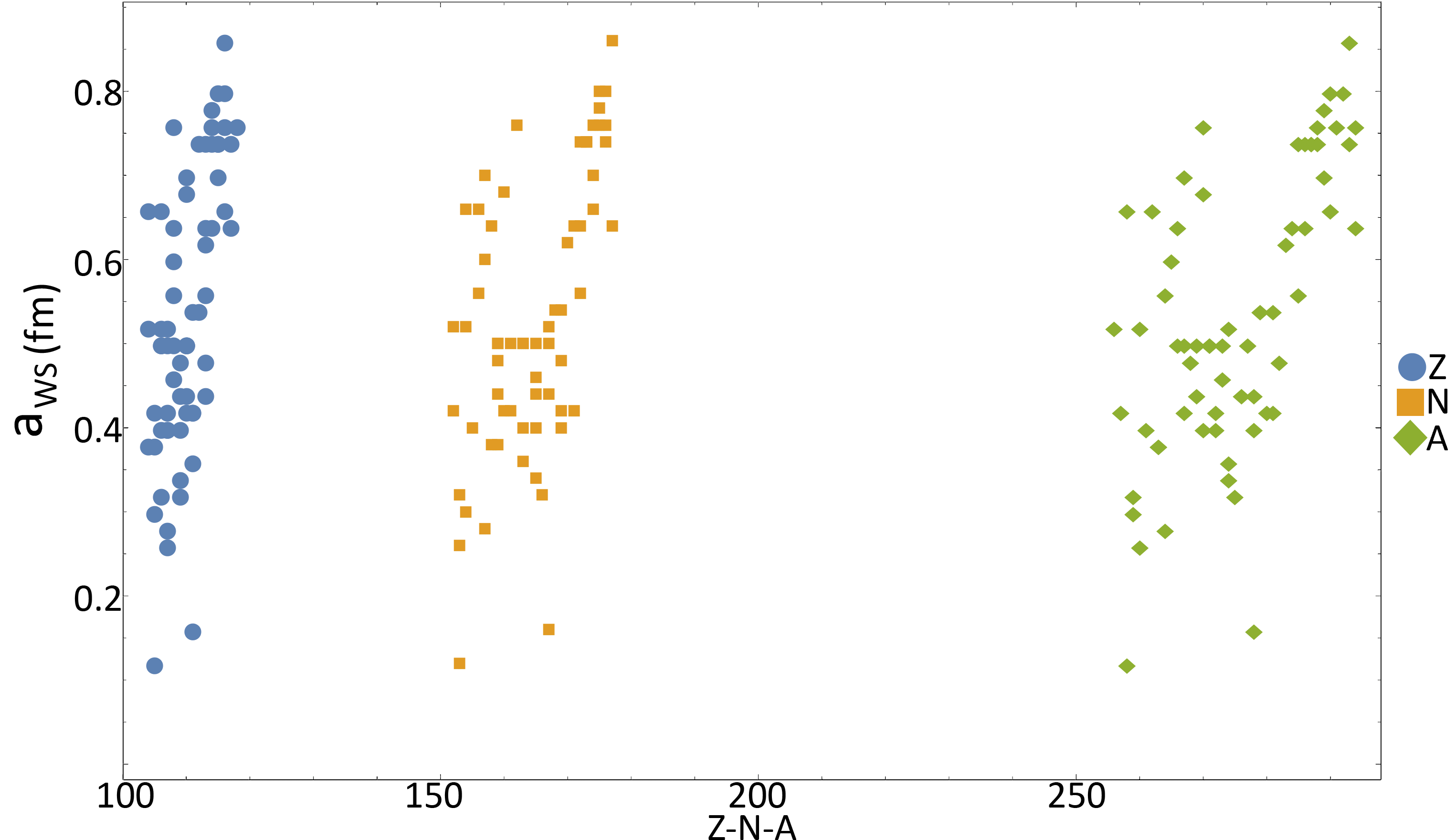
Figure 3: $a_{\text{\tiny WS}}$ (fm) vs $Z,N$, and $A$.

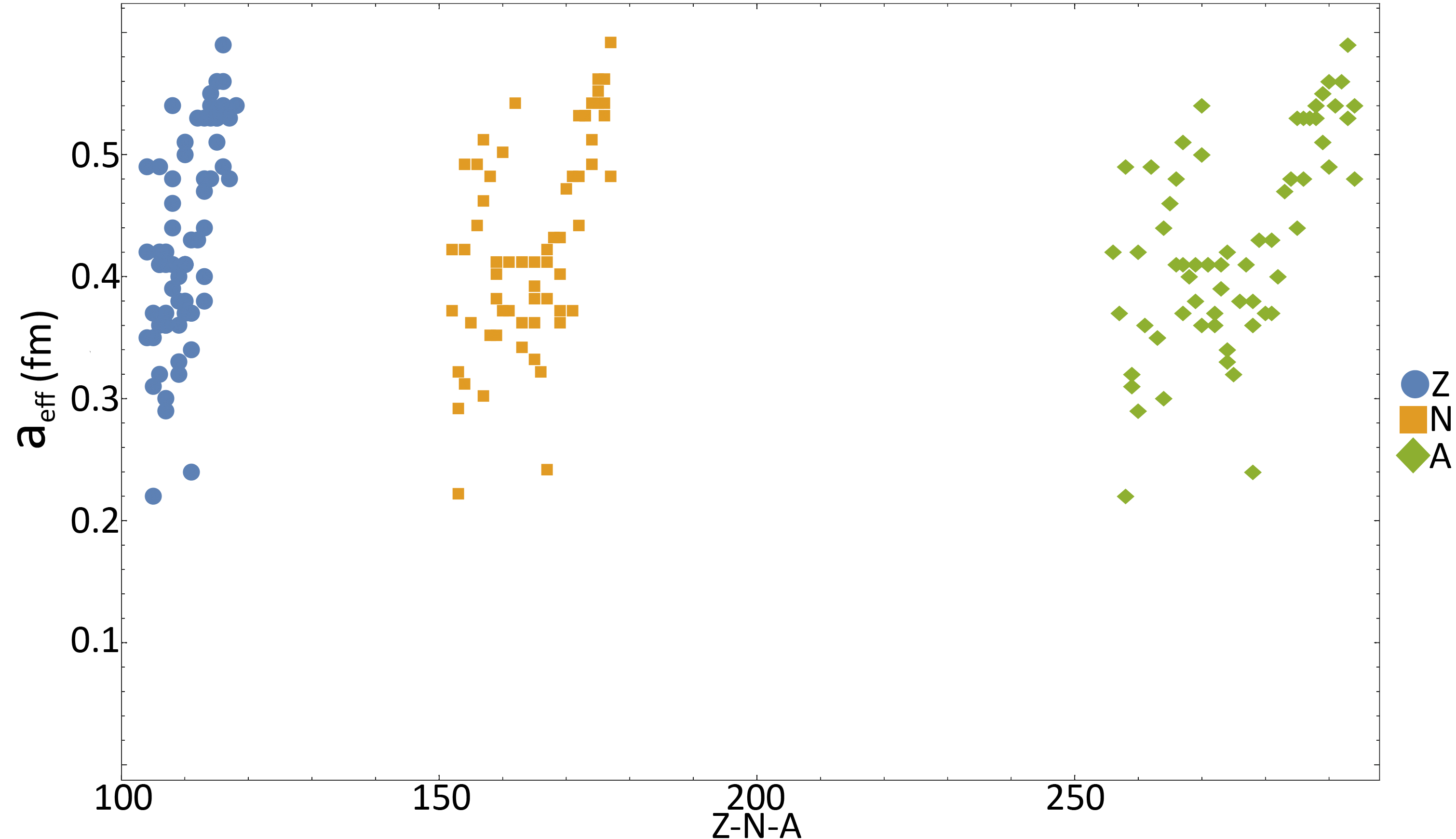
Figure 4: $a_{\text{eff}}$ (fm) vs $Z,N$, and $A$.

1. For $a_{\text{eff}}$, a linear fit best represents the data with an rms error of 0.065 fm from true $a_{\text{eff}}$ values. The obtained semiempirical formula is given by

   $$a_{\text{eff}}=-1.09535+0.012063Z+0.0019759N$$ (15)

2. No fitting model was found for $a_{\text{\tiny WS}}$ that approximate true $a_{\text{\tiny WS}}$ with a reasonable rms error comparable to the one for $a_{\text{eff}}$. In particular, linear and non-linear models produced rms error of around 0.13-0.16 fm whereas adopting constant $a_{\text{\tiny WS}}=0.54$ fm produced rms error of around 0.17 fm.

From comparing the figures, one can understand why it’s easier to find a fit for $a_{\text{eff}}$ in which points are condensed more tightly compared to the more scattered and disperse data for $a_{\text{\tiny WS}}$. Moreover, there’s a stronger $Z$ dependence in both cases compared to $N$ dependence, which is reflected in the fact that the coefficient of $Z$ is one order of magnitude larger than that of $N$.

V Calculations and predictions of $\alpha$ half-lives of 218 SHN

In this section, we calculate and predict $\alpha$ half-lives of 218 SHN based on the theoretical framework outlined earlier and the semiempirical formula proposed. In particular, we calculate half-lives for 68 SHN for which there exists available experimental data using our proximity potential model; for these nuclei we do not use the semiempirical formula but rather compute $a_{\text{eff}}$ directly from $a_{\text{\tiny WS}}$ using the mapping outlined in the previous section; moreover, the results obtained are compared against previous work that assumed deformed WS, deformed Coulomb potentials and constant $a_{\text{\tiny WS}}=0.54$ fm for all nuclei (WS model) [12]. Moreover, we compare our output with the results of six of the most powerful semiempirical formulas. Regarding the 150 SHN whose half-lives to be predicted, there’s no available $a_{\text{\tiny WS}}$ for them and hence we make use of our proposed semiempirical formula to compute $a_{\text{eff}}$ values. Experimental or theoretical $Q_{\alpha}$ values are taken from Refs. [21, 14, 12].

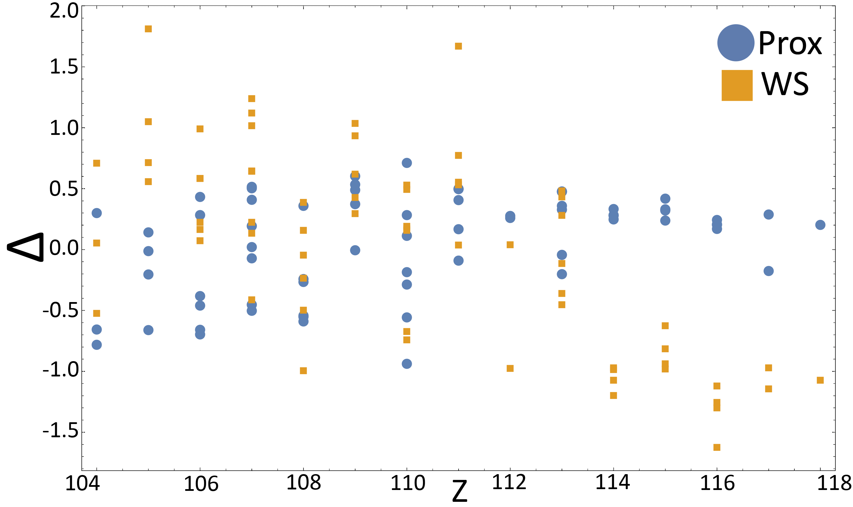
Figure 5: $\Delta_{\text{calc}}$ and $\Delta^{\text{deformed}}_{\text{\tiny WS}}$ plotted vs. charge number $Z$ where they are dubbed prox and WS respectively.

The results of the calculations for the 68 SHN are tabulated in Table 2, where $Z$ varies from 104 to 118 and $N$ varies from 152 to 176. The table also contains the logarithm of errors for our model $\Delta_{\text{calc}}=\log_{10}T_{\text{exp}}-\log_{10}T_{\text{calc}}$ and $\Delta^{\text{deformed}}_{\text{\tiny WS}}=\log_{10}T_{\text{exp}}-\log_{10}T^{\text{deformed}}_{\text{\tiny WS}}$ for the deformed WS, deformed Coulomb model with constant diffuseness. Moreover, a plot of the errors of the two models vs. $Z$ is shown in Fig. 5. We note that one calculation is not included in the table, graphs or earlier fitting procedure, namely, that of 256Db with error $\Delta>1$ for both models. We worked with arbitrary precision in our calculations but rounded up numbers in the tables to the nearest 2 or 3 decimal places. Fig. 5 is instructive to draw conclusions from; in particular, it shows our model–dubbed Prox– performs favorably in several aspects. First, is that most of the points are clustered around the 0.5 to -0.5 band, unlike the WS model which has more disperse points and are equally likely to be found inside and outside the 0.5 band. Second, $|\Delta_{\text{calc}}|<1$ for all points in our model (except 256Db which was mentioned earlier); this is to be contrasted with the results of WS model in which there are more than 21 points exceeding the 1 to -1 band (i.e., $|\Delta^{\text{deformed}}_{\text{\tiny WS}}|>1$) with 3 points even exceeding 1.5 or -1.5. Statistical comparison between the performance of our model (Prox), WS model, and six semiempirical formulas (ImSahu, Sahu, Royer10, VS, SemFIS and UNIV) [21] is shown in Table 3 in which rms, mean, mean deviation and difference between the maximum and minimum errors are shown respectively. The rms of errors is given by $\sqrt{\macc@depth\char 1\relax\frozen@everymath{\macc@group}\macc@set@skewchar\macc@nested@a 111{}}$,

$$\sqrt{\macc@depth\char 1\relax\frozen@everymath{\macc@group}\macc@set@skewchar\macc@nested@a 111{}}=\hbox to0.0pt{\leavevmode\hbox{\set@color$\displaystyle\sqrt{\dfrac{1}{M}{\sum\limits_{i}^{M}\Delta_{i}^{2}}}$}\hss}\hskip 6.99994pt{\raisebox{9.50423pt}{\rule{31.0887pt}{0.49057pt}}}$$ (16)

where $M$ is the number of SHN under study. The mean of errors is simply given by

Table 1: Experimental data $\log_{10}T_{\text{exp}}$ vs. our model Prox $\log_{10}T_{\text{calc}}$ with variable effective diffuseness $a_{\text{eff}}$ vs. $\log_{10}T^{\text{deformed}}_{\text{\tiny WS}}$ deformed Woods-Saxon, deformed Coulomb potentials with constant diffuseness $a_{\text{\tiny WS}}=0.54$ fm. Values for $Q_{\alpha}$ and $\log_{10}T^{\text{deformed}}_{\text{\tiny WS}}$ are from Ref. [12].

$Z$	$N$	$A$	$Q_{\alpha}$	$a_{\text{eff}}$	$b_{\text{eff}}$	$\log_{10}T_{\text{exp}}$	$\log_{10}T_{\text{calc}}$	$\log_{10}T^{\text{deformed}}_{\text{\tiny WS}}$	$\Delta_{\text{calc}}$	$\Delta^{\text{deformed}}_{\text{\tiny WS}}$
104	152	256	8.926	0.42	0.77	0.319	1.093	0.265	-0.770	0.054
104	154	258	9.190	0.49	0.89	-1.035	-0.398	-0.512	-0.645	-0.523
104	159	263	8.250	0.35	0.64	3.301	2.997	2.592	0.311	0.709
105	152	257	9.206	0.37	0.67	0.389	1.039	-0.169	-0.649	0.558
105	153	258	9.500	0.22	0.40	0.776	0.777	-1.036	-0.001	1.812
105	154	259	9.620	0.31	0.57	-0.292	-0.101	-1.341	-0.192	1.049
105	158	263	8.830	0.35	0.64	1.798	1.619	1.056	0.152	0.715
106	153	259	9.804	0.32	0.58	-0.492	-0.043	-1.482	-0.449	0.990
106	154	260	9.901	0.42	0.78	-1.686	-1.001	-1.759	-0.685	0.073
106	155	261	9.714	0.36	0.66	-0.638	-0.268	-1.222	-0.37	0.584
106	156	262	9.600	0.49	0.89	-1.504	-0.855	-0.921	-0.648	0.583
106	163	269	8.700	0.41	0.75	2.079	1.785	1.913	0.294	0.166
106	165	271	8.670	0.41	0.75	2.219	1.775	1.996	0.444	0.223
107	153	260	10.40	0.29	0.53	-1.459	-0.969	-2.698	-0.490	1.239
107	154	261	10.50	0.31	0.57	-1.899	-1.459	-2.916	-0.440	1.017
107	157	264	9.960	0.30	0.55	-0.357	-0.390	-1.479	0.033	1.122
107	159	266	9.430	0.41	0.75	0.23	0.290	0.005	-0.060	0.225
107	160	267	9.230	0.37	0.67	1.23	1.024	0.643	0.206	-0.413
107	163	270	9.060	0.36	0.66	1.785	1.364	1.140	0.421	0.645
107	165	272	9.310	0.36	0.66	1.000	0.474	0.356	0.526	0.644
107	167	274	8.930	0.42	0.77	1.732	1.218	1.598	0.515	0.134
108	156	264	10.591	0.44	0.80	-2.796	-2.219	-2.750	-0.577	-0.046
108	157	265	10.47	0.46	0.84	-2.699	-2.167	-2.464	-0.532	-0.235
108	158	266	10.346	0.48	0.87	-2.638	-2.097	-2.141	-0.54	-0.497
108	159	267	10.037	0.41	0.75	-1.187	-0.956	-1.344	-0.23	0.157
108	162	270	9.050	0.54	0.98	0.556	0.810	1.55	-0.254	-0.994
108	165	273	9.730	0.39	0.71	-0.119	-0.490	-0.506	0.37	0.387
109	159	268	10.67	0.33	0.60	-1.678	-1.684	-2.613	0.006	0.935
109	165	274	10.20	0.32	0.58	-0.357	-0.973	-1.394	0.616	1.037
109	166	275	10.48	0.38	0.69	-1.699	-2.086	-2.127	0.386	0.428
109	167	276	10.03	0.36	0.66	-0.347	-0.848	-0.966	0.501	0.619
109	169	278	9.580	0.40	0.73	0.653	0.106	0.358	0.547	0.295
110	157	267	11.78	0.51	0.93	-5.553	-4.625	-4.811	-0.926	-0.742
110	159	269	11.509	0.38	0.69	-3.747	-3.472	-4.242	-0.275	0.495
110	160	270	11.12	0.50	0.91	-4.00	-3.455	-3.327	-0.545	-0.673
110	161	271	10.899	0.41	0.75	-2.639	-2.465	-2.808	-0.174	0.169
110	163	273	11.38	0.41	0.75	-3.77	-3.894	-3.927	0.124	0.157
110	167	277	10.72	0.41	0.75	-2.222	-2.518	-2.413	0.295	0.191
110	171	281	9.32	0.37	0.67	2.125	1.403	1.596	0.723	0.529
111	161	272	11.197	0.34	0.62	-2.420	-2.338	-3.193	-0.080	0.773
111	163	274	11.48	0.24	0.44	-2.194	-2.7027	-3.864	0.508	1.67
111	167	278	10.85	0.43	0.78	-2.377	-2.557	-2.415	0.180	0.038
111	168	279	10.53	0.37	0.67	-1.046	-1.465	-1.578	0.419	0.532
111	169	280	9.91	0.37	0.67	0.663	0.151	0.111	0.511	0.552
112	169	281	10.46	0.43	0.78	-1.000	-1.288	-1.040	0.287	0.040
112	173	285	9.32	0.53	0.96	1.447	1.175	2.424	0.2715	-0.977
113	165	278	11.85	0.38	0.69	-3.62	-3.589	-4.053	-0.032	0.433
113	169	282	10.78	0.42	0.73	-1.155	-1.525	-1.437	0.370	0.282
113	170	283	10.48	0.47	0.86	-1.00	-0.812	-0.640	-0.189	-0.360
113	171	284	10.12	0.48	0.87	-0.041	-0.382	0.442	0.340	0.483
113	172	285	10.01	0.44	0.80	0.623	0.137	0.738	0.486	-0.115
113	173	286	9.79	0.48	0.87	0.978	0.482	1.431	0.490	-0.453
114	172	286	10.35	0.53	0.96	-0.699	-0.994	0.273	0.294	-0.972
114	173	287	10.17	0.54	0.98	-0.319	-0.610	0.755	0.290	-1.074
114	174	288	10.072	0.55	1.00	-0.180	-0.440	1.018	0.259	-1.198

Table 2: (Continued).

$Z$	$N$	$A$	$Q_{\alpha}$	$a_{\text{eff}}$	$b_{\text{eff}}$	$\log_{10}T_{\text{exp}}$	$\log_{10}T_{\text{calc}}$	$\log_{10}T^{\text{deformed}}_{\text{\tiny WS}}$	$\Delta_{\text{calc}}$	$\Delta^{\text{deformed}}_{\text{\tiny WS}}$
114	175	289	9.98	0.53	0.97	0.279	-0.066	1.264	0.345	-0.985
115	172	287	10.76	0.53	0.97	-1.432	-1.682	-0.451	0.249	-0.981
115	173	288	10.63	0.53	0.97	-1.060	-1.393	-0.121	0.333	-0.939
115	174	289	10.52	0.51	0.93	-0.658	-1.010	0.156	0.342	-0.814
115	175	290	10.41	0.49	0.89	-0.187	-0.614	0.438	0.429	-0.625
116	174	290	10.99	0.54	0.98	-1.824	-2.047	-0.705	0.220	-1.12
116	175	291	10.89	0.56	1.02	-1.721	-1.975	-0.466	0.254	-1.255
116	176	292	10.774	0.59	1.07	-1.745	-1.926	-0.121	0.181	-1.624
116	177	293	10.68	0.56	1.02	-1.276	-1.492	0.024	0.214	-1.300
117	176	293	11.18	0.53	0.97	-1.854	-2.156	-0.883	0.301	-0.971
117	177	294	11.07	0.48	0.87	-1.745	-1.580	-0.601	-0.165	-1.144
118	176	294	11.82	0.54	0.98	-3.161	-3.376	-2.089	0.215	-1.072

$$\macc@depth\char 1\relax\frozen@everymath{\macc@group}\macc@set@skewchar\macc@nested@a 111{}=\dfrac{1}{M}{\sum\limits_{i}^{M}\Delta_{i}}$$ (17)

Mean deviation is given by

$$\macc@depth\char 1\relax\frozen@everymath{\macc@group}\macc@set@skewchar\macc@nested@a 111{}=\dfrac{1}{M}{\sum\limits_{i}^{M}|\Delta_{i}|}$$ (18)

We note that the statistical parameters shown in Table 3 for semiempirical formulas were obtained for 69 SHN in the region $92\leq Z\leq 118$ [21]; owing to the similar sample size and same region for charge number, we conclude that it is reasonable to make a comparison between them and our model. We note that there was no available data for $\macc@depth\char 1\relax\frozen@everymath{\macc@group}\macc@set@skewchar\macc@nested@a 111{}$ and $\Delta_{\text{max}}-\Delta_{\text{min}}$ for the semiempirical formulas. We observe that our model Prox performs better than all models except ImSahu. All in all, these results help to consolidate the importance of diffuseness in half-lives calculations; it shows that using accurate diffuseness parameter is more important than taking deformation into account. Moreover, we note that WS takes two parameters $\beta_{2}$ and $\beta_{4}$ (deformation parameters), while Prox takes only one, namely $a_{\text{eff}}$(If we use our new fitted formula then we take no parameters at all). In addition, it shows the reasonableness of the mapping $a_{\text{eff}}=(a_{\alpha}+a_{\text{\tiny WS}})/2$ proposed earlier. We expect that by incorporating deformation, more accurate preformation factor formula and etc. into our model, we can get even more accurate results.

Table 3: Statistical comparison between our model Prox vs. deformed WS, deformed Coulomb model (WS) vs. ImSahu vs. Sahu vs. Royer10 vs. VS vs. SemFIS vs. UNIV. Data for statistical parameters for semiempirical formulas are taken from Ref. [21].

Model	$\sqrt{\macc@depth\char 1\relax\frozen@everymath{\macc@group}\macc@set@skewchar\macc@nested@a 111{}}$	$\macc@depth\char 1\relax\frozen@everymath{\macc@group}\macc@set@skewchar\macc@nested@a 111{}$	$\macc@depth\char 1\relax\frozen@everymath{\macc@group}\macc@set@skewchar\macc@nested@a 111{}$	$\Delta_{\text{max}}-\Delta_{\text{min}}$
Prox	0.41	0.064	0.36	1.65
WS	0.79	0.01	0.67	3.44
ImSahu	0.362		0.287
Sahu	0.709		0.58
Royer10	0.523		0.429
VS	0.623		0.508
SemFIS	0.504		0.413
UNIV	0.477		0.392

Motivated by these results, we predicted the half-lives of 150 SHN between $105\leq Z\leq 121$ with the aid of our new semiempirical formula for $a_{\text{eff}}$. We will compare our results with seven of the current most powerful semiempirical formulas for $\alpha$ half-lives: Viola-Seaborg (VS), Royer (R), modified Brown 1 (mB1), modified Brown 2 (mB2), ImSahu, SemFIS and UNIV. Half-lives predictions made by these 7 semiempirical formulas which we shall compare our model against are taken from Refs. [14, 21].

Predictions of half-lives for 35 SHN in the region $105\leq Z\leq 118$ are shown in Table 4. The comparison is made between our model Prox, Viola-Seaborg (VS), modified Brown 1 (mB1), Royer (R), and modified Brown 2 (mB2) and the average of the four semiempirical formulas [14]. The results of our model are pretty consistent with the predictions of the four formulas.

Table 4: Our model Prox $\log_{10}T_{\text{calc}}$ vs. Viola-Seaborg $\log_{10}T_{\text{\tiny VS}}$ vs. modified Brown formula 1 $\log_{10}T_{\text{\tiny mB1}}$ vs. Royer $\log_{10}T_{\text{\tiny R}}$ vs. modified Brown formula 2 $\log_{10}T_{\text{\tiny mB2}}$ vs. average of the four semiempirical formulas $\log_{10}T_{\text{avg}}$ and error $\Delta_{\text{avg}}$ between our model and the average. $Q_{\alpha}$ values and half-lives for the semiempirical formulas are from Ref. [14].

$Z$	$N$	$A$	$Q_{\alpha}$	$\log_{10}T_{\text{calc}}$	$\log_{10}T_{\text{\tiny VS}}$	$\log_{10}T_{\text{\tiny mB1}}$	$\log_{10}T_{\text{\tiny R}}$	$\log_{10}T_{\text{\tiny mB2}}$	$\log_{10}T_{\text{avg}}$	$\Delta_{\text{avg}}$
105	159	264	8.95	1.096	1.179	1.181	1.078	1.118	1.139	0.043
106	161	267	9.12	0.790	0.641	0.622	0.666	0.685	0.654	-0.013
106	167	273	8.20	3.493	3.239	3.247	3.367	3.439	3.323	-0.170
108	153	261	10.97	-2.402	-3.164	-3.197	-3.228	-3.335	-3.231	-0.830
108	164	272	9.60	-0.123	-0.558	-0.613	-0.597	-0.562	-0.583	-0.460
108	169	277	8.85	1.910	1.859	1.822	1.88	1.928	1.872	-0.036
110	165	275	10.38	-1.627	-1.483	-1.503	-1.590	-1.573	-1.537	0.090
110	166	276	10.23	-1.310	-1.603	-1.645	-1.749	-1.714	-1.678	-0.369
110	177	278	9.94	-0.651	-0.919	-0.970	-0.952	-0.907	-0.937	-0.287
111	165	276	10.44	-1.434	-1.067	-1.072	-0.983	-1.001	-1.031	0.403
112	160	272	11.20	-2.402	-3.271	-3.257	-3.490	-3.563	-3.395	-0.993
112	161	273	11.06	-2.199	-2.543	-2.517	-2.565	-2.650	-2.569	-0.370
112	162	274	10.92	-1.980	-2.703	-2.703	-2.838	-2.900	-2.786	-0.806
112	163	275	10.79	-1.772	-1.961	-1.949	-1.980	-2.054	-1.986	-0.214
112	164	276	10.65	-1.525	-2.107	-2.120	-2.149	-2.203	-2.145	-0.620
112	165	278	10.37	-0.985	-1.478	-1.507	-1.421	-1.468	-1.469	-0.484
112	166	279	10.23	-0.692	-0.704	-0.721	-0.709	-0.768	-0.726	-0.034
113	167	280	10.69	-1.551	-1.192	-1.170	-1.085	-1.126	-1.143	0.416
114	164	278	11.55	-2.990	-3.594	-3.529	-3.778	-3.814	-3.679	-0.691
114	165	279	11.41	-2.780	-2.876	-2.801	-2.923	-2.961	-2.890	-0.111
114	166	280	11.28	-2.577	-3.047	-3.000	-3.151	-3.180	-3.095	-0.518
114	167	281	11.14	-2.339	-2.315	-2.260	-2.362	-2.394	-2.333	0.006
114	168	282	11.00	-2.086	-2.472	-2.445	-2.491	-2.515	-2.481	-0.390
114	169	283	10.87	-1.845	-1.726	-1.691	-1.770	-1.798	-1.746	0.098
114	170	284	10.73	-1.563	-1.868	-1.862	-1.795	-1.816	-1.835	-0.272
114	171	285	10.59	-1.267	-1.107	-1.093	-1.146	-1.171	-1.129	0.137
115	171	286	11.04	-2.093	-1.566	-1.500	-1.447	-1.455	-1.492	0.600
115	176	291	10.35	-0.549	-0.207	-0.207	-0.224	-0.216	-0.214	0.335
116	171	287	11.50	-2.886	-2.664	-2.554	-2.731	-2.715	-2.666	0.220
116	172	288	11.36	-2.628	-2.832	-2.753	-2.819	-2.808	-2.803	0.175
116	173	289	11.22	-2.356	-2.097	-2.012	-2.164	-2.148	-2.105	0.250
117	175	292	11.4	-2.607	-1.934	-1.812	-1.798	-1.768	-1.828	0.772
118	175	293	11.85	-3.367	-3.010	-2.833	-3.089	-3.020	-2.988	0.378
118	177	295	11.58	-2.847	-2.463	-2.316	-2.545	-2.479	-2.451	0.395

Table 5: Statistical comparison showing how consistent our model Prox is on one hand with VS, mB1, Royer, and mB2 on the other.

Model	$\sqrt{\macc@depth\char 1\relax\frozen@everymath{\macc@group}\macc@set@skewchar\macc@nested@a 111{}}$	$\macc@depth\char 1\relax\frozen@everymath{\macc@group}\macc@set@skewchar\macc@nested@a 111{}$	$\macc@depth\char 1\relax\frozen@everymath{\macc@group}\macc@set@skewchar\macc@nested@a 111{}$	$\Delta_{\text{max}}-\Delta_{\text{min}}$
Prox	0.43	-0.09	0.34	1.77

The most relevant statistical parameters are shown in Table 5. We can see that the values of the parameters are consistent with the ones in Table 3 reassuring us further to the utility and viability of our fit.

Next, we predict the half-lives of 115 SHN in the $118\leq Z\leq 121$ region and compare our results to that of ImSahu, SemFIS and UNIV semiempirical formulas [21]. The predictions are compiled in Table 7. To perform meaningful statistical analysis, we considered logarithm of half-lives values in which the three semiempirical formulas converge within 10$\%$; hence, we define $\epsilon$ as [14],

$$\epsilon=\dfrac{\max(|\log_{10}T_{i}|)-\min(|\log_{10}T_{j}|)}{\max(|\log_{10}T_{i}|)}$$ (19)

where the indices $i$ and $j$ can be 1, 2, and 3 representing ImSahu, SemFIS, and UNIV, respectively. After looking for SHN with $\epsilon<0.1$, we took the average of the three formulas $\log_{10}T_{\text{avg}}=(\log_{10}T_{\text{\tiny ImSahu}}+\log_{10}T_{\text{\tiny SemFIS}}+\log_{10}T_{\text{\tiny UNIV}})/3$ then defined $\Delta_{\text{avg}}=\log_{10}T_{\text{avg}}-\log_{10}T_{\text{calc}}$ to measure consistency of our results with that of the other formulas. The result of this analysis is shown in Table 8. The rms error is 0.526 which is still considered acceptable with current standards.

Table 6: Half-lives calculations for our model Prox $\log_{10}T_{\text{calc}}$ vs. ImSahu $\log_{10}T_{\text{\tiny ImSahu}}$ vs. SemFIS $\log_{10}T_{\text{\tiny SemFIS}}$ vs. UNIV $\log_{10}T_{\text{\tiny UNIV}}$. $Q_{\alpha}$ values and half-lives for the semiempirical formulas are from Ref. [21].

$Z$	$N$	$A$	$Q_{\alpha}$	$\log_{10}T_{\text{calc}}$	$\log_{10}T_{\text{\tiny ImSahu}}$	$\log_{10}T_{\text{\tiny SemFIS}}$	$\log_{10}T_{\text{\tiny UNIV}}$
118	160	278	13.89	-5.693	-6.69	-7.32	-7.26
118	161	279	13.78	-5.668	-8.25	-6.44	-6.4
118	162	280	13.71	-5.705	-6.46	-6.90	-6.99
118	163	281	13.76	-5.948	-8.14	-6.31	-6.40
118	164	282	13.49	-5.606	-6.15	-6.42	-6.64
118	165	283	13.33	-5.447	-7.32	-5.46	-5.68
118	166	284	13.23	-5.389	-5.75	-5.87	-6.21
118	167	285	13.07	-5.207	-6.77	-4.91	-5.24
118	168	286	12.92	-5.029	-5.25	-5.2	-5.67
118	169	287	12.8	-4.900	-6.19	-4.35	-4.76
118	170	288	12.62	-4.636	-4.75	-4.62	-5.12
118	171	289	12.59	-4.668	-5.71	-3.93	-4.39
118	172	290	12.6	-4.775	-4.77	-4.59	-5.11
118	173	291	12.42	-4.479	-5.30	-3.60	-4.08
118	174	292	12.24	-4.167	-4.12	-3.87	-4.42
118	175	293	12.24	-4.231	-4.85	-3.28	-3.74
118	176	294	11.82	-3.355	-3.30	-3.02	-3.53
118	177	295	11.9	-3.585	-4.06	-2.62	-3.05
118	178	296	11.75	3.285	-3.21	-2.97	-3.43
118	179	297	12.1	-4.106	-4.41	-3.19	-3.51
118	180	298	12.18	-4.307	-4.19	-4.06	-4.39
118	181	299	12.05	-4.041	-4.22	-3.23	-3.44
118	182	300	11.96	-3.852	-3.79	-3.76	-3.95
118	183	301	12.02	-3.990	-4.08	-3.36	-3.41
118	184	302	12.04	-4.030	-4.03	-4.13	-4.16
118	185	303	12.6	-5.213	-5.18	-4.77	-4.62
118	186	304	13.12	-6.227	-6.20	-6.49	-6.32
118	187	305	12.91	-5.792	-5.69	-5.59	-5.25
118	188	306	12.48	-4.885	-5.05	-5.52	-5.12
118	189	307	11.92	-3.631	-3.63	-3.90	-3.28
118	190	308	12.2	-4.200	-2.34	-3.10	-2.35
119	161	280	14.3	-6.224	-7.32	-6.51	-6.30
119	162	281	14.16	-6.154	-7.26	-6.97	-6.96
119	163	282	14	-6.038	-6.90	-5.90	-5.84
119	164	283	13.76	-5.766	-6.60	-6.19	-6.32
119	165	284	13.57	-5.566	-6.24	-5.05	-5.14
119	166	285	13.61	-5.777	-6.34	-5.84	-6.10
119	167	286	13.43	-5.575	-6.06	-4.73	-4.92
119	168	287	13.28	-5.415	-5.76	-5.17	-5.54
119	169	288	13.23	-5.435	-5.77	-4.31	-4.59
119	170	289	13.16	-5.408	-5.54	-4.91	-5.35
119	171	290	13.07	-5.334	-5.54	-3.98	-4.33
119	172	291	13.05	-5.388	-5.02	-3.35	-3.74
119	173	292	12.9	-5.176	-4.78	-4.20	-4.69
119	174	293	12.72	-4.890	-4.59	-2.19	-3.28
119	175	294	12.73	-4.891	-4.90	-3.33	-3.52
119	185	304	12.93	-5.677	-5.71	-4.39	-4.28
119	186	305	13.42	-6.609	-5.97	-6.15	-6.07
119	187	306	13.2	-6.172	-6.27	-5.10	-4.82
119	188	307	12.78	-5.316	-4.80	-5.18	-4.91
119	189	308	12.06	-3.752	-4.11	-3.11	-2.59
119	190	309	11.37	-2.097	-1.81	-2.49	-1.92
120	163	283	14.31	-6.238	-9.02	-6.87	-6.83
120	164	284	13.99	-5.843	-6.45	-6.91	-7.01

Table 7: (Continued).

$Z$	$N$	$A$	$Q_{\alpha}$	$\log_{10}T_{\text{calc}}$	$\log_{10}T_{\text{\tiny ImSahu}}$	$\log_{10}T_{\text{\tiny SemFIS}}$	$\log_{10}T_{\text{\tiny UNIV}}$
120	165	285	13.89	-5.818	-8.25	-6.05	-6.17
120	166	286	14.03	-6.211	-6.58	-6.88	-7.11
120	167	287	13.85	-6.029	-8.11	-5.90	-6.13
120	168	288	13.73	-5.942	-6.15	-6.28	-6.63
120	169	289	13.71	-6.028	-7.79	-5.59	-5.92
120	170	290	13.7	-6.124	-6.16	-6.18	-6.61
120	171	291	13.51	-5.880	-7.36	-5.19	-5.60
120	172	292	13.47	-5.905	-5.82	-5.74	-6.24
120	173	293	13.4	-5.865	-7.09	-4.98	-5.43
120	174	294	13.24	-5.644	-5.47	-5.31	-5.85
120	175	295	13.27	-5.779	-6.77	-4.76	-5.23
120	176	296	13.34	-5.983	-5.72	-5.54	-6.06
120	177	297	13.14	-5.659	-6.46	-4.55	-5.02
120	178	298	13.01	-5.457	-5.18	-4.97	-5.48
120	179	299	13.26	-5.994	-6.60	-4.87	-5.27
120	180	300	13.32	-6.149	-5.81	-5.66	-6.09
120	181	301	13.06	-5.676	-6.15	-4.59	-4.93
120	182	302	12.89	-5.361	-5.08	-4.95	-5.31
120	183	303	12.81	-5.216	-5.60	-4.23	-4.48
120	184	304	12.76	-5.123	-4.89	-4.84	-5.09
120	185	305	13.28	-6.158	-6.40	-5.31	-5.40
120	186	306	13.79	-7.102	-6.82	-6.95	-7.01
120	187	307	13.52	-6.594	-6.74	-5.94	-5.86
120	188	308	12.97	-5.512	-5.42	-5.65	-5.56
120	189	309	12.16	-3.779	-4.05	-3.51	-3.25
120	190	310	11.5	-2.211	-2.41	-2.82	-2.48
121	165	286	14.34	-6.279	-7.31	-7.26	-5.96
121	166	287	14.53	-6.752	-7.56	-7.53	-7.15
121	167	288	14.46	-6.778	-7.56	-7.37	-6.18
121	168	289	14.4	-6.813	-7.36	-7.23	-6.97
121	169	290	14.42	-6.976	-7.56	-7.24	-6.15
121	170	291	14.4	-7.064	-7.35	-7.18	-7.00
121	171	292	14.31	-7.024	-7.45	-7.01	-6.00
121	172	293	14.1	-6.766	-6.86	-6.63	-6.54
121	173	294	14.1	-6.865	-7.17	-6.63	-5.69
121	174	295	13.98	-6.744	-6.66	-6.42	-6.37
121	175	296	14.01	-6.881	-7.08	-6.48	-5.57
121	176	297	14.12	-7.152	-6.89	-6.68	-6.64
121	177	298	13.89	-6.812	-6.94	-6.30	-5.39
121	178	299	13.65	-6.435	-6.09	-5.88	-5.86
121	179	300	13.81	-6.783	-6.87	-6.21	-5.29
121	180	301	13.82	-6.847	-6.38	-6.27	-6.19
121	181	302	13.49	-6.275	-6.38	-5.71	-4.75
121	182	303	13.31	-5.962	-5.48	-5.42	-5.31
121	183	304	13.28	-5.928	-6.06	-5.43	-4.40
121	184	305	13.27	-5.925	-5.40	-5.48	-5.27
121	185	306	13.81	-6.948	-7.06	-6.55	-5.38
121	186	307	14.34	-7.883	-7.23	-7.54	-7.15
121	187	308	14.07	-7.409	-7.55	-7.17	-5.85
121	188	309	13.26	-5.896	-5.38	-5.81	-5.31
121	189	310	12.46	-4.238	-4.66	-4.34	-2.89
121	190	311	11.81	-2.747	-2.44	-3.06	-2.37

Table 8: Measure of consistency of our model Prox with that of ImSahu, SemFIS, and UNIV.

Model	$\sqrt{\macc@depth\char 1\relax\frozen@everymath{\macc@group}\macc@set@skewchar\macc@nested@a 111{}}$	$\macc@depth\char 1\relax\frozen@everymath{\macc@group}\macc@set@skewchar\macc@nested@a 111{}$	$\macc@depth\char 1\relax\frozen@everymath{\macc@group}\macc@set@skewchar\macc@nested@a 111{}$	$\Delta_{\text{max}}-\Delta_{\text{min}}$
Prox	0.526	-0.013	0.4217	2.46

VI Discussion and conclusions

The present analysis and results leave us with several conclusions and remarks:

• The effect of diffuseness can no longer be ignored by adopting it as a constant for all SHN; even very slight variations as small as 0.1 fm can induce an error in half-life as large as 0.69; this is especially true for systems which we expect to have large diffuseness; the effect is especially pronounced when proximity potential is adopted in which we find non-linear (convex) variation of the logarithm of half-life with diffuseness; we conclude that diffuseness is a great bottleneck acting as a limiting factor against accurate half-lives calculations.

• Present calculations and comparisons show that taking true values of diffuseness parameter into account is more critical than deformation effects; this was shown when we compared our model with WS model.

• The use of the mapping $a_{\text{eff}}=(a_{\alpha}+a_{\text{\tiny WS}})/2$ produced results for 68 SHN that are in great agreement with available experimental data; it outperformed all models except the ImSahu model. This shows the viability and utility of this mapping, which can be adopted for future use.

• Our predictions of $\alpha$ half-lives of 150 SHN using our newly proposed fitted formula is in good agreement with other semiempirical formulas; this is especially true for the region $105\leq Z\leq 118$ which was the region of the original fit. By using a bigger sample size over a more extended region, a semiempirical formula better than the one at hand can be produced to be used in half-lives calculations.

• For our predictions, we did not incorporate centripetal contribution $V_{l}(r)$ due to the lack of information about angular momentum of the systems under study. Incorporating these data will improve the accuracy of the results.

• Present investigations and calculations show that $a_{\text{eff}}$ is best represented as a linear function of charge and neutron numbers.

• Present calculations corroborate the viability of the Prox model; we expect that by taking further effects into account including deformation, more accurate parity-dependent preformation factor and etc., the errors will be reduced even further.

• A potentially fruitful research direction is to investigate the role of diffuseness in half-life using other models for nuclear potential.

• We stress that future research should invest an appreciable amount of energy in calculating and extracting accurate diffuseness parameters values.

References

- Ismail et al. [2017] M. Ismail, W. M. Seif, A. Adel, and A. Abdurrahman, Nucl. Phys. A. 958, 202 (2017).
- Basu [2003] D. N. Basu, Phys. Lett. B 566, 90 (2003).
- Ren et al. [2004] Z. Ren, C. Xu, and Z. Wang, Phys. Rev. C 70, 034304 (2004).
- Royer and Moustabchir [2001] G. Royer and R. Moustabchir, Nucl. Phys. A 683, 182 (2001).
- Zhang et al. [2013] G. L. Zhang, H. B. Zheng, and W. W. Qu, Eur. Phys. J. A 49, 10 (2013).
- Yao et al. [2015] Y. J. Yao, G. L. Zhang, W. W. Qu, and J. Q. Qian, Eur. Phys. J. A 51, 122 (2015).
- Zhang et al. [2011] H. F. Zhang, G. Royer, and J. Q. Li, Phys. Rev. C 84, 027303 (2011).
- Denisov and Ikezoe [2005] V. Y. Denisov and H. Ikezoe, Phys. Rev. C 72, 064613 (2005).
- Xu and Ren [2005] C. Xu and Z. Ren, Nucl. Phys. A 760, 303 (2005).
- Xu and Ren [2006] C. Xu and Z. Ren, Phys. Rev. C 74, 014304 (2006).
- Sun et al. [2017] X. D. Sun, J. G. Deng, D. Xiang, P. Guo, and X. H. Li, Phys. Rev. C 95, 044303 (2017).
- Dehghani et al. [2018] V. Dehghani, S. A. Alavi, and K. Benam, Mod. Phys. Lett. A 33, 1850080 (2018).
- Guo et al. [2015a] C. L. Guo, G. L. Zhang, and M. Li, Int. J. Mod. Phys. E 24, 1550040 (2015a).
- Budaca et al. [2016] A. I. Budaca, R. Budaca, and I. Silisteanu, Nucl. Phys. A 951, 60 (2016).
- Guo et al. [2015b] S. Guo, X. Bao, Y. Gao, J. Li, and H. Zhang, Nucl. Phys. A 934, 110 (2015b).
- Zheng et al. [2013] L. Zheng, G. L. Zhang, J. C. Yang, and W. W. Qu, Nucl. Phys. A 915, 70 (2013).
- Błocki et al. [1977] J. Błocki, J. Randrup, W. J. Świa¸tecki, and C. F. Tsang, Ann. Phys. (NY) 105, 427 (1977).
- Myers and Świa¸tecki [2000] W. D. Myers and W. J. Świa¸tecki, Phys. Rev. C 62, 044610 (2000).
- Möller and Nix [1981] P. Möller and J. R. Nix, Nucl. Phys. A 361, 117 (1981).
- Gupta et al. [2009] R. K. Gupta, D. Singh, R. Kumar, and W. Greiner, J. Phys. G: Nucl. Part. Phys. 36, 075104 (2009).
- Zhang et al. [2017] S. Zhang, Y. Zhang, J. Cui, and Y. Wang, Phys. Rev. C 95, 014311 (2017).