The phase diagram of the Hubbard model by Variational Auxiliary Field quantum Monte Carlo

Abstract

A systematically improvable wave function is proposed for the numerical solution of strongly correlated systems. With a stochastic optimization method, based on the auxiliary field quantum Monte Carlo technique, an effective temperature $T_{\mathrm{eff}}$ is defined, probing the distance of the ground state properties of the model in the thermodynamic limit from the ones of the proposed correlated mean-field ansatz. In this way their uncertainty from the unbiased zero temperature limit may be estimated by simple and stable extrapolations well before the so called sign problem gets prohibitive. At finite $T_{\mathrm{eff}}$ the convergence of the energy to the thermodynamic limit is indeed shown to be possible in the Hubbard model already for relatively small square lattices with linear dimension $L\simeq 10$, thanks to appropriate averages over several twisted boundary conditions. Within the estimated energy accuracy of the proposed variational ansatz, two clear phases are identified, as the energy is lowered by spontaneously breaking some symmetries satisfied by the Hubbard Hamiltonian: a) a stripe phase where both spin and translation symmetries are broken, and b) a strong coupling d-wave superconducting phase when the particle number is not conserved and global $U(1)$ symmetry is broken. On the other hand the symmetric phase is stable in a wide region at large doping and small coupling.

I Introduction

The accurate numerical solution of the Schroëdinger equation, namely determining the ground state of a many-body Hamiltonian $H$, remains the most challenging unsolved problem since the Dirac’s formulation in 1931. Historically, important progress, as well as too optimistic promises, occurs periodically at least twice a decade, starting from quantum computers, the Density Functional Theory Kohn-Sham formulationKohn and Sham (1965), the Density Matrix Renormalization Group (DMRG)White (1992); Schollwöck (2005) and its translation within the tensor network quantum information languageOrús (2014); Verstraete et al. (2004); Schuch et al. (2011), wrong claimsSorella et al. (1989); Corney and Drummond (2004); Efetov et al. (2009) about the solution of the sign problem in Quantum Monte Carlo (QMC), systematically improvable wave functions (WFs) based on multi reference expansionsBooth et al. (2013); Dobrautz et al. (2019); Yao et al. (2020) or on machine learning assumptionsCarleo and Troyer (2017); Carleo et al. (2019), just to mention a few of them.

Unfortunately, determining the exact ground state of a strongly correlated Hamiltonian $H$ in the thermodynamic limit, remains an open issue apart for particular cases as in one dimensionLieb and Wu (1968) or with very particular couplingsKitaev (2006). Also for this reason, the Hubbard model has been historically used to benchmark new techniques, because its simplicity represents an ideal playground for advanced computational and also experimental methods such as optical latticesMazurenko et al. (2017).

As far as the 2D Hubbard model is concerned only a few results have been established by numerical techniques, namely a clear antiferromagnetic phase at one electron per site fillingHirsch (1985); Seki and Sorella (2019); LeBlanc et al. (2015) is present and a strong evidence that this phase remains even when this condition is not fulfilledZheng et al. (2017): the added holes (unoccupied sites) are expelled from the antiferromagnet, and essentially fill in equally spaced vertical lines of the lattice: the so called stripes.

Instead, the question of superconductivity in the Hubbard model remains highly debated and controversial since the discovery of high-temperature superconductivityZhang et al. (1997); Maier et al. (2005); Deng et al. (2015) to the last few monthsQin et al. (2020). Probably the most clear evidence of superconductivity was reported in the strong coupling limit of the Hubbard model, the so called t-J model. Several years ago, this model has been studiedSorella et al. (2002) with an almost standard variational Monte Carlo method (VMC) that simply relies on the variational principle: the best wave function ansatz, defined by a set of variational parameters, is the one that minimizes the expectation value of the Hamiltonian studied. At that time, soon after the discovery of high-temperature superconductivity, it was reported that superconductivity did not need electron-phonon interaction but the driving force was rather the superexchange spin interaction $J$. The approach and especially the claim has been highly debated and remains controversial until now, even though it is worth mentioning that several years later, by tensor network, P. Corboz et al. have reported, without emphasizing it, almost the same value of the off-diagonal $d-wave$ superconducting long range order.

Despite this success and its simplicity, the standard VMC based on a single reference mean-field ansatz, e.g. the Hartree-Fock (HF), corrected by a simple correlation term, e.g. the Gutzwiller factor, is certainly limited as compared with the most recent and advanced variational methods, that allow a systematically improvable ansatz.

In this work, a different strategy is proposed to overcome the limitations of correcting a simple mean-field ansatz for reaching accurate ground state properties. The approach will be dubbed in the following variational auxiliary field quantum Monte Carlo (VAFQMC), that takes advantage of the enormous progress done in the last decades by two old but well established techniques: the variational quantum Monte Carlo (VMC) and the auxiliary field quantum Monte Carlo (AFQMC)Becca and Sorella (2017); Umrigar et al. (2007); Sorella et al. (1989); White et al. (1989); Loh et al. (1990). From the former technique its simplicity and clarity in interpreting the results in the thermodynamic limit as well as its ability to optimize a mean-field state $\psi_{MF}$ in presence of a simple correlated factor are taken. Conversely from AFQMC a systematically convergent and non perturbative expression of the correlation term is used. Indeed AFQMC allows the application of $\exp(-H\tau/2)$ to any mean-field state, where $\tau$ is the total imaginary time used in this formulation. Thus, the projection $\exp(-H\tau/2)$ filters out exactly the ground state component of $\psi_{MF}$ for large imaginary time $\tau$, yielding that the ansatz $|\psi_{\tau}\rangle_{0}=\exp(-H\tau/2)|\psi_{MF}\rangle$, basically used in this work, represents a systematically improvable- with increasing $\tau$- correlated mean-field ansatz, retaining all advantages of the two mentioned formalisms.

The simple working hypothesis of this study is the following. Suppose that, in the thermodynamic limit, the mean-field wave function has acquired the lowest possible energy upon breaking some symmetry of the Hamiltonian in presence of an enough accurate correlation term. In this case, the implicit VMC assumption is that the exact ground state should eventually show this phase. On the other hand, with the proposed method one can in principle tune the accuracy of the electron correlation at the desired level and verify explicitly the systematic evolution of the phase diagram, derived in this way, from the simplest mean-field HF theory ($\tau=0$) to the converged one. This limit can be approached very closely at half-filling. Unfortunately, for the finite doping case, the exact ($\tau=\infty$) limit cannot be met in principle because the method presented here is vexed by the so called sign problem. Nevertheless extremely accurate variational energies can be obtained even with short $\tau$ projection.

In short the high energy degrees of freedom (e.g. the average number of doubly occupied sites) of the variational ansatz are settled almost immediately with short $\tau$ projection (e.g. they are filtered out with the projection with an exponetial decay proportional to a large gap $\simeq U$). As long as the low energy degrees of freedom and the high energy ones are almost decoupled, an hypothesis implicitly assumed in several theoretical and computational methods in physics and chemistry, the phase diagram derived with this ansatz should converge fast with $\tau$, because only the high energy degrees of freedom have to be settled by the projection.

II Model and wave function

In this work, the square lattice Hubbard model $H=K_{\mu}+V$ is studied, where $K_{\mu}=\sum_{k,\sigma}c^{\dagger}_{k,\sigma}c_{k,\sigma}(-2t(\cos k_{x}+\cos k_{y})-\mu)$ is the kinetic energy, defined here by the hopping $t$ and the chemical potential $\mu$ and $V=U\sum_{i}n_{\uparrow,i}n_{\downarrow,i}$ is the total number of doubly occupied sites operator scaled by the coupling $U>0$ of the model, where standard second quantization notations are assumed. We introduce the following ansatzEichenberger and Baeriswyl (2007); Yanagisawa et al. (1998); Yanagisawa (2016), also inspired by similar wave functions quite popular in quantum computationBeach et al. (2019); Wecker et al. (2015), with the purpose to reach accurate ground state properties in the shortest possible projection time $\tau$:

$$|\psi_{\tau}\rangle=\exp\left[-{\tau\over 2}(H_{MF}(\bm{\alpha})+V)\right]|\psi_{MF}\rangle.$$ (1)

As shown later, the above variational wave function represents a straightforward improvement of the standard auxiliary field QMC one $|\psi_{\tau}\rangle_{0}$, mentioned in the introduction. The mean-field wave function $|\psi_{MF}\rangle$ can be a generic quasi-free electron state, from a simple Slater determinant to BCS pairing functions, including singlet and/or triplet correlations. Here, $|\psi_{MF}\rangle$ is allowed breaking some symmetries of the Hamiltonian, and is defined as the ground state of a mean-field Hamiltonian $H_{MF}(\bm{\alpha_{0}})$, i. e. $H_{MF}(\bm{\alpha_{0}})|\psi_{MF}\rangle=E_{0}(\bm{\alpha_{0}})|\psi_{MF}\rangle$ with a set of variational parameters indicated by the vector $\bm{\alpha_{0}}$. For the projection operator, we take the advantage of the variational formulation, so that any extension of the variational ansatz containing a given one- i.e. $|\psi_{\tau}\rangle_{0}$- as a particular case should necessarily improve it, namely after energy optimization, acquires a lower variational energy. The bare kinetic energy operator in $\exp(-H\tau/2)$ is therefore generalized (i.e. $K_{\mu}\to H_{MF}(\bm{\alpha})$), by allowing a generic operator quadratic in the fermion ones $c,c^{\dagger}$, including for instance also a d-wave BCS pairing field. $H_{MF}(\bm{\alpha})$ is therefore parameterized by a set of variational parameters indicated by another independent vector $\bm{\alpha}$, such that for $\bm{\alpha}=0$ $H_{MF}(\bm{\alpha})=K_{\mu}$. In other words the idea is that if a symmetry is broken in the thermodynamic limit also the projection operator, i.e. the correlation factor, and not only the mean-field state $|\psi_{MF}\rangle$ may break the symmetry and therefore $H_{MF}(\bm{\alpha})$ is conveniently parametrized in a way similar to $\psi_{MF}$.

This original formulation improves the quality of the ansatz and the smooth convergence to the thermodynamic limit, as compared with the simpler ansatz $|\psi_{\tau}\rangle_{0}$ and the optimal energy is therefore generally obtained after the simultaneous optimization of both $\bm{\alpha}$ and $\bm{\alpha_{0}}.$

We anticipate that, in this variational formulation of the auxiliary field quantum Monte Carlo (VAFQMC), $\tau$ plays the role of an effective inverse temperature that is kept fixed during the minimization of the energy expectation value corresponding to $|\psi_{\tau}\rangle$.

The optimization techniques known in standard variational Monte CarloSorella (1998) and machine learningAmari (1998) will be generalized here to the auxiliary field QMC. Before that, it is worth to emphasize simple but important properties of this ansatz:

1. It is systematically improvable. In order to realize this property, it is enough to take $\bm{\alpha}=0$, when the proposed ansatz coincides with the simpler one $|\psi_{\tau}\rangle_{0}=\exp(-H\tau/2)|\psi_{MF}\rangle$. Thus, let $\tau\to\infty$ for a mean field $|\psi_{MF}\rangle$ of the chosen form, that is not orthogonal to the ground state. In this limit $|\psi_{\tau}\rangle_{0}$ is obviously converging to the exact ground state. Thus, after turning on optimization, by allowing both $\bm{\alpha}\neq 0$ and, independently, $\bm{\alpha_{0}}$ different from the initial guess, a lower energy is necessarily implied for each $\tau$, yielding that the ansatz of Eq. 1 is systematically improvable, as well as and even better than $|\psi_{\tau}\rangle_{0}$ as far as its energy is concerned.

2. It is size extensive. As discussed in Ref.Becca and Sorella, 2017 the WF is defined directly in terms of an exponential of an extensive operator, hence the statement. In practice this means that, at a given $\tau$, approximately the same accuracy for intensive quantities is expected, e.g. the energy per site or bulk correlation functions.

3. For finite clusters the convergence is exponential in $\tau$ due to the finite size gap between the ground state manifold (which may be also degenerate) and the first excitation with non zero energy gap. However in the thermodynamic limit this gap is probably always vanishing in this model, even for the half filled insulator, where gapless spin-wave excitations are expected due to the occurrence of antiferromagnetic order for any $U>0$Seki and Sorella (2019). This situation, as it will be shown in the following, makes the extrapolation to the ${1\over\tau}=0$ unbiased limit much simpler than the corresponding finite size case. Indeed this can be obtained by simple and stable low order polynomial extrapolations in something that can be considered an effective temperature $T_{\mathrm{eff}}=1/\tau$.

The key idea of this work is to converge first the results to the thermodynamic limit with large enough cluster size simulations and appropriate boundary conditions. Given this, simple and very stable extrapolations in $T_{\mathrm{eff}}\to 0$ are employed, thus achieving, with this simple minded strategy, very accurate results of the model or at least an estimate of the accuracy of the lowest $T_{\mathrm{eff}}$ variational ansatz. As presented later, this is often possible because, after the optimization, the physical properties of the ansatz given in Eq.(1) are already in the very low temperature regime, where the mentioned extrapolations are indeed stable and reliable within a given broken symmetry phase.

It is well establishedFisher (1989); Hasenfratz and Niedermayer (1993); Hofmann (2010) that, when a standard type of order that breaks a continuous symmetry sets in, the corresponding gapless low energy excitations (i.e. typically bosons with a density of states $\rho(\epsilon)\propto\epsilon^{D-1}$) induce $\simeq T^{3}$ ($\simeq T^{2}$) energy corrections (i.e. $\Delta E\propto\int\limits_{0}^{T}\epsilon\rho(\epsilon)\simeq T^{D+1}$) in the limit $T\to 0$ for 2D (quasi 1D system like a finite cylinder with infinite length), and indeed it turns out that the fit

$$E(T_{\mathrm{eff}})=E(0)+aT_{\mathrm{eff}}^{D+1}+bT_{\mathrm{eff}}^{D+2}$$ (2)

is generally very appropriate for the systems studied here, because the available $T_{\mathrm{eff}}$ appear always quite close to the correct asymptotic behavior. A formal derivation of the finite effective temperature corrections is given in App.A.

Given the above arguments, particularly useful boundary conditions are adopted such that the convergence to the thermodynamic limit at fixed $\tau$ is as fast as possible. To this purpose twisted averaged boundary conditions TABCLin et al. (2001); Gros (1996) are used in both the Hubbard Hamiltonian and the mean-field ones on rectangular $L_{x}\times L_{y}$ clusters ($L_{x}=L_{y}=L$ is adopted for square lattices). This is obtained by imposing opposite twists for opposite spins:

$$c_{r_{x}+L_{x},r_{y},\uparrow} = c_{r_{x},r_{y},\uparrow}\exp(i2\pi\theta_{x})$$

$$c_{r_{x},r_{y}+L_{y},\uparrow} = c_{r_{x},r_{y},\uparrow}\exp(i2\pi\theta_{y})$$

$$c_{r_{x}+L_{x},r_{y},\downarrow} = c_{r_{x},r_{y},\downarrow}\exp(-i2\pi\theta_{x})$$

$$c_{r_{x},r_{y}+L_{y},\downarrow} = c_{r_{x},r_{y},\downarrow}\exp(-i2\pi\theta_{y})$$

with $\theta_{x}=-1/2+(i-1/2)/N_{T}$ and $\theta_{y}=-1/2+(j-1/2)/N_{T}$ for integers $1\leq i,j\leq N_{T}$, while $r_{x}$ and $r_{y}$ here and henceforth indicate integer Cartesian coordinates of the lattice $1\leq r_{x}\leq L_{x}$, $1\leq r_{y}\leq L_{y}$. All the results are then averaged on a mesh of $N_{T}\times N_{T}$ twists in the Brillouin zone (BZ), with $N_{T}$ large enough to have converged energies within statistical errors. When $H_{MF}$ conserves the number of particles $N$ and has a gap in the one particle spectrum, $N$ remains unchanged for each twist, whereas when a BCS pairing is present, grand canonical ensemble is adopted as discussed in Ref.Karakuzu et al., 2018 and the expectation value of $H-\mu\hat{N}$ is minimized by the proposed variational ansatz, where $\hat{N}=\sum\limits_{r_{x},r_{y},\sigma}c^{\dagger}_{r_{x},r_{y},\sigma}c_{r_{x},r_{y},\sigma}$ is the particle number operator.

The use of opposite twists for opposite spin electrons is particularly important in this case because it allows the conservation of the translation symmetry in the BCS mean-field Hamiltonian, at least in a simple way.

Before explaining how to optimize the variational parameters it is useful to appreciate in Fig. 1 the fast and smooth convergence of the grand potential $\Omega={\langle\psi_{\tau}|H-\mu\hat{N}|\psi_{\tau}\rangle\over\langle\psi_{\tau}|\psi_{\tau}\rangle}$ in the thermodynamic limit as a function of the number $N_{s}$ of sites for a value of the chemical potential corresponding to doping $\delta=1-N/N_{s}\approx 1/8$.

Figure 1: Grand potential per site $\Omega/N_{s}$ as a function of cluster size for different values of the projection time $\tau$ for $\mu=1.75t$ and $U/t=8$

The other important ingredient for an efficient implementation of Eq. (1) is the use of a particularly suited Trotter decomposition for the corresponding propagator:

$$\exp\left[-{\tau\over 2}(H_{MF}(\bm{\alpha})+V)\right]=$$

$$\left\{\prod\limits_{i=1}^{n}\exp\left[-t_{i}H_{MF}(\bm{\alpha})\right]\exp\left[-h_{i}V\right]\right\}\times$$

$$\exp\left[-t_{n+1}H_{MF}(\bm{\alpha})\right]$$ (4)

where in principle $h_{i}$ and $t_{i}$ can be independently optimized to minimize the Trotter error, as proposed in a recent workBeach et al. (2019). Henceforth it is assumed that the operators in Eq. (II) are ordered from left to right according to increasing values of the integer $i$. In this work $\tau$ is kept fixed, and therefore the following constraint is imposed:

$$\sum\limits_{i=1}^{n}h_{i}={\tau\over 2}.$$ (5)

Moreover, in order to minimize the number of variational parameters and the number $n$, the following parameterization is adopted:

$$h_{i} = \Delta\tau\gamma^{i-1}$$ (6)

$$t_{i} = {h_{i}+h_{i-1}\over 2}~{}~{}{\rm for}~{}i=1,2,\cdots n$$ (7)

with $h_{0}=0$ and $\gamma>1$ chosen in a way to satisfy the constraint in Eq. (5). This expression is based on the conventional small $\Delta\tau$ symmetric Trotter decomposition $\exp\left[-{\Delta\tau}(H_{MF}(\bm{\alpha})+V)\right]=\exp\left[-{\Delta\tau\over 2}H_{MF}(\bm{\alpha})\right]\exp\left[-\Delta\tau V\right]\exp\left[-{\Delta\tau\over 2}H_{MF}(\bm{\alpha})\right]+O(\Delta\tau^{3})$, where a nonuniform time step according to Eq. (6) has been chosen because, for high accuracy, it is important only that the first time step is small and $\gamma\simeq 1$. In this way the efficiency and the number of operators involved is significantly optimized, without using too many variational parameters as in Ref.Beach et al., 2019. In all forthcoming calculations only a single parameter $\Delta\tau$ is optimized with the convenient choice:

$$n={\rm Max}\left\{[(\tau U/0.4-1)/5],1\right\},$$ (8)

leading to a Trotter time step error on the energy that, for all $U$ values reported, can be hardly distinguished from the error bars. Here and henceforth the square brackets indicate the integer part of a real number.

III Variational Auxiliary Field Method

Since $H_{MF}(\bm{\alpha})$ is a one body operator and $|\psi_{MF}\rangle$ is a mean-field state (e.g. a Slater determinant) there is no difficulty to apply $\exp\left[-t_{i}H_{MF}\bm{(}\alpha)\right]$ to $|\psi_{MF}\rangle$. Moreover, taking into account that $\exp\left[-t_{i}H_{MF}\bm{(}\alpha)\right|\psi_{MF}\rangle$ remains a mean-field state, this operation can be also performed iteratively.

The application of $\exp(-h_{i}V)$ is instead more complicated and can nevertheless be implemented by using the auxiliary field technique. To this purpose the following discrete Hubbard-Stratonovich transformationHirsch (1985) is used:

$$\exp(-h_{i}V)=2^{-N_{s}}\exp(-Uh_{i}\hat{N}/2)\sum\limits_{\sigma_{j,i}=\pm 1}\exp(\lambda_{i}\sum\limits_{j}\sigma_{ji}m_{j})$$ (9)

where $m_{j}=n_{j,\uparrow}-n_{j,\downarrow}$, $\hat{N}$ is the total number of particles operator, $\cosh\lambda_{i}=\exp(Uh_{i})$ and the Ising variables $\sigma_{ji}=\pm 1$ for each site $j$ of the lattice. Notice that the factor $\exp(-Uh_{i}\hat{N}/2)$ represents only an irrelevant change of the chemical potential in $H_{MF}(\bm{\alpha})$. Therefore this term is omitted for simplicity here and henceforth.

We get therefore that the expectation value of Hamiltonian $H$ (or any relevant correlation function) for the wave function in Eq.(1) is given by:

$$E_{n} = {\langle\psi_{n}|H|\psi_{n}\rangle\over\langle\psi_{n}|\psi_{n}\rangle}$$ (10)

$$= {\sum\limits_{\bm{\sigma}\bm{\sigma^{\prime}}}\langle\psi_{MF}|U^{\dagger}_{n}(\bm{\sigma^{\prime}})HU_{n}(\bm{\sigma})|\psi_{MF}\rangle\over\sum\limits_{\bm{\sigma}\bm{\sigma^{\prime}}}\langle\psi_{MF}|U^{\dagger}_{n}(\bm{\sigma^{\prime}})U_{n}(\bm{\sigma})|\psi_{MF}\rangle}$$ (11)

where $\bm{\sigma}$ indicates the $N_{s}\times n$ dimensional vector with components $\sigma_{ji}$, and:

$$U_{n}(\bm{\sigma}) =\exp(-H_{MF}(\bm{\alpha})t_{1})\exp(\lambda_{1}\sum_{j}\sigma_{j,1}m_{j})$$

$$\cdots \exp(-H_{MF}(\bm{\alpha})t_{n})\exp(\lambda_{n}\sum_{j}\sigma_{j,n}m_{j})\exp(-H_{MF}(\bm{\alpha})t_{n+1})$$

$E_{n}$ can be therefore computed by Monte Carlo, by sampling the Ising fields $\bm{\sigma}$ and $\bm{\sigma^{\prime}}$ according to the weight $|W_{n}(\bm{\sigma^{\prime}},\bm{\sigma})|$, where:

$$W_{n}(\bm{\sigma^{\prime}},\bm{\sigma})=\langle\psi_{MF}|U^{\dagger}_{n}(\bm{\sigma^{\prime}})U_{n}(\bm{\sigma})|\psi_{MF}\rangle$$ (13)

and, quite generally in the complex case, $W_{n}$ has a non trivial phase that is determined by $S_{n}(\bm{\sigma^{\prime}},\bm{\sigma})={W_{n}(\bm{\sigma^{\prime}},\bm{\sigma})\over|W_{n}(\bm{\sigma^{\prime}},\bm{\sigma})|}$, a complex number with unit modulus, that plays the role of the QMC sign.

Finally $E_{n}$ can be computed by :

$$E_{n}={\sum\limits_{\bm{\sigma}\bm{\sigma^{\prime}}}|W_{n}(\bm{\sigma^{\prime}},\bm{\sigma})|e_{n}(\bm{\sigma^{\prime}},\bm{\sigma})S_{n}(\bm{\sigma^{\prime}},\bm{\sigma})\over\sum\limits_{\bm{\sigma}\bm{\sigma^{\prime}}}|W_{n}(\bm{\sigma^{\prime}},\bm{\sigma})|S_{n}(\bm{\sigma^{\prime}},\bm{\sigma})}$$ (14)

namely by evaluating the ratio of the means corresponding to two real random variables $\Re[e_{n}(\bm{\sigma^{\prime}},\bm{\sigma})S_{n}(\bm{\sigma^{\prime}},\bm{\sigma})]$ and $\Re[S_{n}(\bm{\sigma^{\prime}},\bm{\sigma})]$ over the configurations generated by Monte Carlo sampling according to the probability $p_{n}(\bm{\sigma^{\prime}},\bm{\sigma})={|W_{n}(\bm{\sigma^{\prime}},\bm{\sigma})|\over\sum\limits_{\bm{\sigma}\bm{\sigma^{\prime}}}|W_{n}(\bm{\sigma^{\prime}},\bm{\sigma})|}$, using the standard technique described in Ref.Becca and Sorella, 2017, and:

$$e_{n}(\bm{\sigma^{\prime}},\bm{\sigma})={\langle\psi_{MF}|U^{\dagger}_{n}(\bm{\sigma^{\prime}})HU_{n}(\bm{\sigma})|\psi_{MF}\rangle\over W_{n}(\bm{\sigma^{\prime}},\bm{\sigma})}$$ (15)

is a sort of local energy, namely an estimate of $E_{n}$ for a given configuration of the Ising fields $\bm{\sigma}$ and $\bm{\sigma^{\prime}}$. Indeed both $e_{n}(\bm{\sigma^{\prime}},\bm{\sigma})$ and $S_{n}(\bm{\sigma^{\prime}},\bm{\sigma})$, as well as $W_{n}(\bm{\sigma^{\prime}},\bm{\sigma})$ can be computed in $\propto N_{s}^{3}n$ operations because they involve essentially imaginary time propagations of mean-field states under time dependent one body propagators $U_{n}(\bm{\sigma})$ and $U_{n}(\bm{\sigma^{\prime}})$.

The basic ingredient introduced in this work is the possibility to compute energy derivatives of $E_{n}$ with respect to all the parameters defining the WF, i.e. $\bm{\alpha}$ and $\bm{\alpha^{\prime}}$, henceforth assumed to be defined by the 2p variational parameters $\alpha_{1},\alpha_{2},\cdots\alpha_{2p}$ and the minimum time step used $\Delta\tau=\alpha_{2p+1}$ at fixed $\tau$, according to Eq.(5). A simple algebra, very similar to the one known for VMC, implies that any energy derivative ${\partial E_{n}\over\partial\alpha_{j}}$ with respect to an arbitrary variational parameter $\alpha_{j}$, for $j=1,2,\cdots 2p+1$, can be computed by means of corresponding derivatives of two complex functions ${\partial e_{n}\over\partial\alpha_{j}}$, $O_{j}={\partial\ln(W_{n})\over\partial\alpha_{j}}={\partial W_{n}\over\partial\alpha_{j}}/W_{n}$ of the local energy and the logarithm of the weight, respectively:

$${\partial E_{n}\over\partial\alpha_{j}}={\langle\langle\Re\{S_{n}\left[{\partial e_{n}\over\partial\alpha_{j}}+(e_{n}-E_{n})O_{j}\right]\}\rangle\rangle\over\langle\langle\Re(S_{n})\rangle\rangle}$$ (16)

where here and henceforth the symbol $\langle\langle*\rangle\rangle$ indicates the average of the generic random variable $*$ over the probability distribution $p_{n}$ defined before, and for shorthand notations the dependence on $\bm{\sigma}$ and $\bm{\sigma^{\prime}}$ of all the quantities involved is not explicitly shown.

The differentiation of the complex quantities $\ln W_{n}$ and $e_{n}$, required for the ${\partial E_{n}\over\partial\alpha_{j}}$ evaluation, at given values of $\bm{\sigma}$ and $\bm{\sigma^{\prime}}$, may appear very cumbersome and involved especially considering that, it is often necessary, as in VMC, to optimize several parameters. This task can be easily achieved in a computational time equal to the one required to compute the complex quantities $\ln(W_{n})$ and $e_{n}$, remarkably only up to a small prefactor regardless how large is the number of variational parameters involved. This is possible by using Adjoint Algorithmic Differentiation (AAD)Griewank (2000), a technique that is becoming popular in the field of Machine Learning with another name, i.e. ”back propagation”, but was certainly known before in applied mathematicsGriewank (2012), and only recently has been appreciated in physicsSorella and Capriotti (2010); Liao et al. (2019). Once all energy derivatives $\partial_{j}E$ are known, the usual scheme adopted in VMC can be applied also here. Variational parameters are changed according to the equation:

$$\delta\bm{\alpha}=-{\rm rate_{learning}}F^{-1}{\partial E\over\partial\bm{\alpha}}$$ (17)

where ${\rm rate_{learning}}$ is a suitable small constant, determining the speed of convergence to the minimum and $F$ is the so called Fisher-information matrix, given by:

$$F_{ij}=\langle\langle{\partial\log p_{n}\over\partial\alpha_{i}}{\partial\log p_{n}\over\partial\alpha_{j}}\rangle\rangle=\langle\langle\langle\Re(O_{i})\Re(O_{j})\rangle\rangle\rangle$$ (18)

where the symbol $\langle\langle\langle AB\rangle\rangle\rangle=\langle\langle AB\rangle\rangle-\langle\langle A\rangle\rangle\langle\langle B\rangle\rangle$ indicates here the covariance of two random variables over the probability $p_{n}$. We adopt here ${\rm rate_{learning}}\simeq 6$ and the same regularization with $\epsilon=0.01$ described in Ref. Becca and Sorella (2017) to avoid instabilities in the calculation of the inverse matrix. Typically convergence is reached with a few hundreds iterations and, variational parameters are averaged after convergence for about $50$ steps.

IV Testing the method

In this section the proposed method is tested against known benchmark results on infinite systems. Unfortunately there are only a few results available in the thermodynamic limit, and those ones are mainly limited to ground state energies. Nevertheless they are extremely relevant for a variational method, because its predictions can be supported by a good estimate of the energy.

First VAFQMC is tested at $U/t=8$ on cylinders with finite width $L_{y}$ and periodic boundary conditions (PBC) in the short $y-$ direction, in order to compare with the very accurate results determined by DMRG with open boundary conditions (OBC) in the $x-$direction, and extrapolated to the one dimensional $L_{x}=\infty$ thermodynamic limit. As it is seen in Fig. 3 VAFQMC is in very good agreement with the known results for $L_{y}\leq 6$, especially when the $T_{\mathrm{eff}}^{2}\to 0$ extrapolation is employed in a relatively small $L_{y}\times 16$ cluster with $32$ twists in the long direction. In this picture we can also appreciate the importance to use appropriate boundary conditions to reach the thermodynamic limit, as OBC require very large clusters for this purpose, a clear limitation that prevents a very accurate extrapolation. Notice that VAFQMC extrapolated results, though affected by a visible non linear term, are obtained with variational energies that are better (below) than the available DMRG ones also for the smallest width $L_{y}=4$. This is remarkable because DMRG has obviously best performances in almost one dimensional systems. The small discrepancy between VAFQMC and DMRG extrapolated values for $L_{y}=6$ does not necessarily imply that VAFQMC is less accurate in this case, but may be due to the limitation of DMRG in obtaining reliable extrapolations as soon as we approach the 2D case, as also shown by the large error bar reported. In any case it is clear that the proposed extrapolations, can be used to estimate the quality of the VAFQMC best (lowest $T_{\mathrm{eff}}$) variational energy estimates.

In all these VAFQMC calculations, at doping $\delta=1/8$ it has been found that the $W=8$ stripe is the most favorable mean-field, as shown in Fig. 2 for the $L_{y}=4$ case.

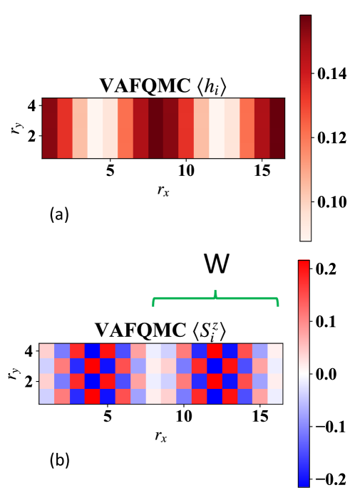
Figure 2: Hole density (a) and spin density (b) for the stripe of width $W=8$ and $U/t=8$ for the $4\times 16$ cluster obtained by energy optimization at $\tau t=1.5$. The green bracket emphasizes the length $W$ of the stripe, i.e. the distance between two domain walls.

Here this state is parametrized by the most general mean-field Hamiltonian with local and nearest neighbor couplings independent of $r_{y}$ (see also the Supplementary Information):

$$H_{MF}(\bm{\alpha_{0}}) = \sum\limits_{r_{x},r_{y},\sigma}\left[-t_{x}(r_{x})c^{\dagger}_{r_{x}+1,r_{y},\sigma}c_{r_{x},r_{y},\sigma}\right.$$ (19)

$$- \left.t_{y}(r_{x})c^{\dagger}_{r_{x},r_{y}+1,\sigma}c_{r_{x},r_{y},\sigma}+{\rm h.c.}\right]$$

$$+ \sum\limits_{r_{x},r_{y}}\Delta_{AF}(r_{x})(-1)^{r_{x}+r_{y}}(n_{\uparrow,r_{x},r_{y}}-n_{\downarrow,r_{x},r_{y}})$$

$$- \mu(r_{x})n_{r_{x},r_{y}}$$

where $n_{\uparrow,r_{x},r_{y}}=c^{\dagger}_{\uparrow,r_{x},r_{y}}c_{\uparrow,r_{x},r_{y}}$, $n_{\downarrow,r_{x},r_{y}}=c^{\dagger}_{\downarrow,r_{x},r_{y}}c_{\downarrow,r_{x},r_{y}}$, $n_{r_{x},r_{y}}=n_{\uparrow,r_{x},r_{y}}+n_{\downarrow,r_{x},r_{y}}.$ Thus the local magnetic antiferromagnetic field satisfies $\Delta_{AF}(r_{x})=-\Delta_{AF}(r_{x}+W)$ and the corresponding local chemical potential $\mu({r_{x}})=\mu(r_{x}+W)$. Moreover nearest neighbor hoppings $t_{x}(r_{x})=t_{x}(r_{x}+W)$ and $t_{y}(r_{x})=t_{y}(r_{x}+W)$ are also included, amounting to a total of $4W$ variational parameters defining $H_{MF}(\bm{\alpha_{0}})$. All their values are assumed independent of the twistsKarakuzu et al. (2018). The few parameter choice adopted in Ref.Tocchio et al., 2019 is used only to initialize the present most general $8W+1$ (by including also the optimization of $H_{MF}(\bm{\alpha})$ and $\Delta\tau$) parameter ansatz $|\psi_{\tau}\rangle$.

For the uniform solution (see Sec. VI) antiferromagnetic order is allowed only at half filling while at finite doping a four (three) parameter ansatz is adopted in $H_{MF}(\bm{\alpha})$ ($H_{MF}(\bm{\alpha_{0}})$, here $t=1$ can be left unchanged, as it sets the scale of the mean-field energy, irrelevant for $|\psi_{MF}\rangle$) including nearest and next nearest neighbor hoppings as well has a uniform chemical potential $\mu_{0}$ and $d_{x^{2}-y^{2}}$ pairing. In all the forthcoming calculations, when the particle number is not defined neither in the mean-field wave function nor in the projection, the energy per site $e(\delta)$ at fixed doping $\delta$ is accurately estimated by an appropriate choice of the chemical potential $\mu$. This is obtained by simple and stable interpolations with a few calculations in the grand canonical ensemble or, in other words, by inverting the Legendre transform from chemical potential dependence to the conjugate density one $1-\delta$.

With this method it is therefore possible to compute the energy in the thermodynamic limit of true 2D clusters without particular effort as the average (complex-) sign $\langle\langle S_{n}\rangle\rangle$ is always larger than $\simeq 0.3$ for all the simulations reported in this work. It is important to remark that, when the 2D-thermodynamic limit is approached, a small but systematic increase of the energy can be appreciated, confirming that, in order to determine the correct two-dimensional thermodynamic limit, true two-dimensional clusters have to be used.

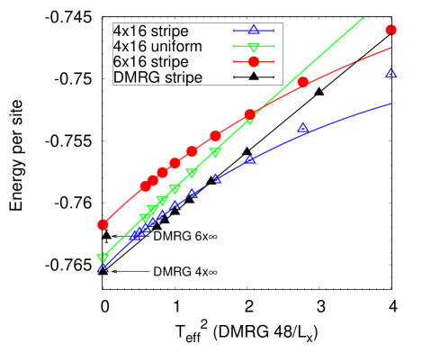
Figure 3: Energy as a function of the effective temperature $T_{\mathrm{eff}}=1/\tau$ for cylinders with different widths. Values at zero horizontal axis result from extrapolations. Here the $D=1$ asymptotic form of Eq. 2 is adopted for the fit of the data in the range $0.7\leq\tau t\leq 1.3$. This form is compatible with the expected low energy spectrum (see text) while the range used is found to be appropriate for $U=8t$ in all cases, included the 2D ones, studied in this work. DMRG energies obtained with open boundary conditions are reported as a function of the inverse cylinder length $L_{x}$ for the $4\times L_{x}$ case, while the extrapolated ones at $L_{x}=\infty$ for both the $4\times L_{x}$ and $6\times L_{x}$ cases.

For $L_{y}$ small the stripe solution is clearly favored as compared with the uniform solution, as found by DMRG. In Fig. 3 the uniform solution is optimized with a non zero $d_{x^{2}-y^{2}}$ BCS pairing but remains clearly above the stripe solution even after extrapolation to $T_{\mathrm{eff}}=0$.

However the situation is quite different when the two-dimensional thermodynamic limit is required. In this case, in order to compare the stripe with periodicity $W=8$ and $W=7$ and the uniform $d-wave$ solution, calculations on a $16\times 16$ and $14\times 16$ clusters are carried out with $16\times 16$ different twists in the BZ. For the $d-$wave ansatz several calculations at different chemical potentials $\mu\simeq 1.8t$ are attempted in order to fulfill a doping $\delta=1/8$ for each effective temperature $T_{\mathrm{eff}}$.

It is seen from the Fig. 4 that in 2D the uniform solution turns out to have an energy competitive with the stripe ones, though the $W=7$ stripe appears to be the most stable solution also because it provides always the lowest variational energy for each $T_{\mathrm{eff}}$. Nevertheless the stripe-uniform phase energy difference, reached at the lowest $T_{\mathrm{eff}}$ shown, is very small $\simeq 0.001t$, though the two variational states remain with qualitatively different types of correlation functions, i.e. a sizable magnetic moment in the former and non negligible $d-wave$ pairing correlations in the latter (see inset in Fig. 4).

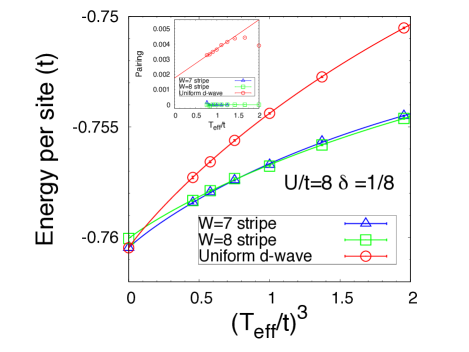
Figure 4: Energy per site at doping $\delta=1/8$ and $U/t=8$ for the stripe solution of different lengths and the uniform $d-wave$ superconducting one, corresponding to the same doping. Values at zero horizontal axis result from extrapolations. Here the $D=2$ fitting form of Eq. 2 is adopted, that is compatible with the expected low energy spectrum (see text). A $16\times 16$ square lattice was used for the $W=8$ stripe and the uniform $d-$wave states while a $14\times 16$ rectangular lattice for the $W=7$ stripe. The inset shows the pairing correlations at maximum horizontal distance $L_{x}/2.$

In Tab. 1 the various extrapolated and best variational energies are compared with the available benchmark resultsLeBlanc et al. (2015); Zheng et al. (2017); Tocchio et al. (2019) obtained with other variational methods. Remarkably VAFQMC provides always the best known variational energies in the thermodynamic limit. In 2D the VAFQMC performances are manifestly excellent if compared with other variational methods, because DMRG becomes rapidly inaccurate with increasing $L_{y}$, and the best variational energy obtained by iPEPS is significantly higher than the VAFQMC one. This may explain why the iPEPS extrapolated energy has a large uncertainty and is much below the VAFQMC and DMRG $6\times\infty$ ones. It is also possible that the extrapolation in the bond dimension is quite inaccurate, and can be substantially improvedCorboz et al. (2018).

Method	$4\times\infty$	$6\times\infty$	$\infty\times\infty$
VMC+backflow Tocchio et al. (2019)	==	-0.7483(1)	-0.74884(1)
DMRG∗Zheng et al. (2017)	-0.76598(3)	-0.7627(5)	==
DMRG∗Chung and White (2018)	-0.7655(1)	==	==
DMRGChung and White (2018)	-0.761826	==	==
iPEPSCorboz (2017)	==	==	-0.75333
iPEPS∗Zheng et al. (2017)	==	==	-0.767(2)
This work	-0.76276(5)	-0.75867(3)	-0.75842(5)
This work∗	-0.7654(1)	-0.7618(1)	-0.7605(1)

Table 1: Best variational energies and extrapolated energies (methods marked by ^∗) for various methods as compared with VAFQMC (last raws) for the $U/t=8$ Hubbard model at $\delta=1/8$. The numbers in parenthesis represent error bars or uncertainties in the extrapolations in the last digit. Other quantum chemistry methods, using also multi reference (MR) expansion, have be shown ”the need for a much larger MR expansion than that afforded"LeBlanc et al. (2015).

Finally the energy and magnetic order parameter are compared at half-filling. In this case there is no sign problem and in principle large imaginary times can be employed without particular difficulties. However, $\tau t\leq 1.3$ has been chosen also in this case, in order to show the strength of this approach even when short time projections are employed. For the order parameter finite effective temperature scaling analysis implies convergence linear in $T_{\mathrm{eff}}$ much slower than the energy (see App.A). Nevertheless remarkably accurate results can be obtained in both cases, as shown in Fig. 5. At finite effective temperature $T_{\mathrm{eff}}$ very weak finite size effects are seen, showing once more the great advantage to use TABC with this approach. The error in the $T_{\mathrm{eff}}\to 0$ extrapolated energy is then compatible with the reference one within the error bars (this work extrapolation $E_{h}=-0.52443(14)$, reference $-0.5247(2)$) whereas the extrapolated order parameter ($0.2894(16)$) is in very good agreement with the benchmark one ($0.2991(2)$).

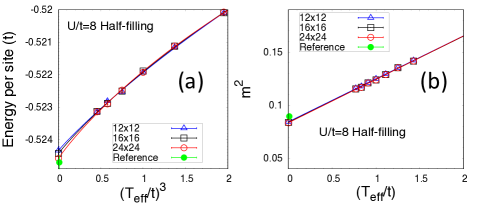
Figure 5: Energy per site (a) and spin-spin correlation function at maximum distance (b) converging to the square antiferromagnetic order parameter $m^{2}$ in the thermodynamic limit. All calculations refer to half-filling and are shown as a function of the effective temperature $T_{\mathrm{eff}}=1/\tau$. Values at zero horizontal axis result from extrapolations. The estimated exact reference values in the thermodynamic limit are taken from Ref.LeBlanc et al., 2015 for the energy and Ref.Seki and Sorella, 2019 for $m$.

V The Hartree-Fock stripe phase

Also within the Hartree-Fock, namely by considering a simple Slater determinant or also uncorrelated BCS mean-field wave functions, very few established results are known, if we allow also nonuniform solutionsSchulz (1990); Xu et al. (2011), i.e. non translation invariant solutions with large unit cell. At half filling it is clear that the simple antiferromagnetic solution, with two site per unit cell, is stable for any $U>0$ as it has been shown analytically by HirschHirsch (1985). On the other hand it is well-known that no superconducting solution is possible for $U>0$. Restricting the solution to a small unit cell containing only two sites leads to a phase separation instabilityEmery et al. (1990), namely the energy per hole:

$$e_{h}(\delta)={\left(e(\delta)-e(0)\right)\over\delta}$$ (20)

acquires a minimum at a finite doping $\delta_{c}$ and for any doping $\delta\leq\delta_{c}$ it is more convenient to expel the holes from a pure antiferromagnet with energy per site $e(0)$ in a region with appropriate size containing an hole rich phase at doping $\delta_{c}$. After this construction (see e.g. App.B) $e_{h}(\delta)$ will be constant in the thermodynamic limit and equal to $e_{h}(\delta_{c})$ for all dopings $\delta\leq\delta_{c}$. This represents a fingerprint of phase separation and the study of the energy per hole can be also considered an implicit way to build a nonuniform solution (when a minimum is found) within not only HF but any variational approach based on a translationally invariant ansatz.

However a better way to expel holes from an antiferromagnet is found by means of the stripe solution already reported in Fig. 2. In particular when the doping $\delta=1/W$ the HF bands show a clear insulating behavior because the unit cell $2\times 2W$ contains $4W$ doubly-degenerate bands and $2W-2$ are fully occupied, as is the case for $\delta=1/8$ shown in Fig. 6. The insulating nature of this stripe solution was also pointed out in weak coupling HF theory by H. SchulzSchulz (1990) who discovered first the stability of incommensurate magnetic states with finite wavevector $Q=(\pi\pm\pi\delta,\pi)$ close to the antiferromagnetic one $Q=(\pi,\pi)$, and the opening of a full gap away from half filling within HF. The occurrence of a finite gap in this case is easily understood not only because the mean-field HF Hamiltonian turns out to have a gap, but also for the following simple general argument holding also in the correlated case. This incommensurate state is adiabatically connected to the insulator having equally spaced empty (i.e. with no-electrons) vertical lines of sites separating half-filled antiferromagnetic insulating regions.

In this way the HF solution can avoid phase separation but the corresponding energy per hole is almost flat at small doping (see Fig. 7a) that is almost equivalent to phase separation. Indeed at small doping the stripes are very far apart $W={1\over\delta}$ and do not interact at all, as can be appreciated in Fig. 7b where the interaction between two vertical stripes at distance $W$ is given by $I(W)=e_{h}(\delta=1/W)-e_{h}(\delta=1/\infty)$. $I(W)$ here defined represents the energy cost per hole for two stripes being at finite distance $W$ rather than at infinite distance, where they do not interact.

At non commensurate doping, for instance $1/8<\delta<1/7$ it is possible to verify that such kind of insulating solutions at $\delta=1/7$ and $\delta=1/8$ can be joined together by forming a smooth doping dependent insulating stripe phase at any intermediate doping (see for instance Fig.7a for $U/t=8$). Many stripes at positions $r_{x_{i}}$ of the lattice can be thought to interact by means of a pairwise repulsive interaction $\propto\sum\limits_{i<j}I(r_{x_{i}}-r_{x_{j}})$, with interaction $I(W)$ as the one computed in Fig. 7b. Thus the rule for obtaining the minimum HF energy is as follows: in order to get the appropriate hole density $\delta$ one alternates energetically more expensive defect stripes of length $W$ smaller than $[1/\delta+1]$ ($W=7$ in this case) by placing them as far as possible.

Figure 6: Hartree-Fock bands for the $W=8$ stripe at $U/t=8$ and doping $\delta=1/8$. There are 32 different bands and only the lowest energy $14$ bands are completely occupied at this filling, implying insulating behavior, as the Fermi energy (blue line) clearly separates the lowest occupied bands from the empty ones. Here $\Gamma=(0,0)$,$X=(\pi/16,0)$ and $M=(\pi/16,\pi/2)$.

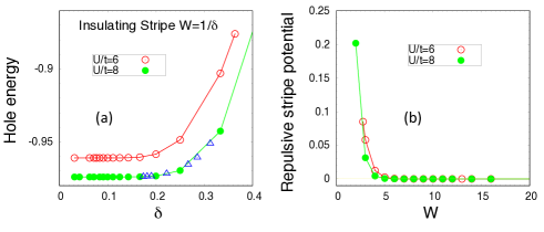
Figure 7: Hole energy (a) for the stripe of width $W$ commensurate with the doping $\delta$ within Hartree-Fock. The blue triangles for $U/t=8$ correspond to intermediate dopings obtained by applying the composition rule described at the end of Sec. V. (b) Effective repulsion energy between equally spaced vertical stripes as a function of their distance $W$.

VI Results for the correlated phase diagram

The rule determined in the previous section to identify the minimum energy insulating stripe solution has been verified also in the correlated case up to the maximum $\tau$ possible with essentially no sign problem, namely $\tau t=1.3,1.73,2.6$ for $U/t=8,6,4$, respectively. Therefore first the stripe wave function (breaking translation and spin symmetry) is computed at commensurate doping $\delta=1/W$, where $W$, being the distance between equally spaced stripes, is an integer. Then, in order to account for intermediate dopings, the corresponding energies are interpolated. Moreover, in order to estimate the error to the exact $T_{\mathrm{eff}}=0$ limit, the results are extrapolated to this limit. Hence the lowest energy of the uniform solution is estimated, that is parametrized by the following mean-field Hamiltonian:

$$H_{MF}(\bm{\alpha_{0}}) = \bar{K}-\mu_{0}\hat{N}+\left[\Delta_{AF}\sum_{R}(-1)^{r_{x}+r_{y}}c^{{\dagger}}_{R,\uparrow}c_{R,\downarrow}\right.$$

$$+ \left.2\Delta_{x^{2}-y^{2}}\sum_{k}(\cos k_{x}-\cos k_{y})c^{{\dagger}}_{k,\uparrow}c^{{\dagger}}_{-k,\downarrow}+{\rm h.c.}\right]$$

where $\bar{K}=\sum\limits_{i,j,\sigma}t_{R,R^{\prime}}c^{\dagger}_{R,\sigma}c_{R^{\prime},\sigma}$ is the translation invariant kinetic energy defined here by the nearest and next nearest neighbor hopping $t$ and $t^{\prime}$, namely $t_{R,R^{\prime}}=-t$ ($t_{R,R^{\prime}}=-t^{\prime}$) if $R$ and $R^{\prime}$ are (next) nearest neighbor sites, $\Delta_{x^{2}-y^{2}}$ determines the gap function for a $d_{x^{2}-y^{2}}$ BCS superconductor, $\Delta_{AF}$ is the mean-field gap due to a commensurate antiferromagnetic state, and $\mu_{0}$ is the mean-field chemical potential value.

By the proposed energy optimization method, as the doping is decreased clear evidence of an instability towards $d_{x^{2}-y^{2}}$ BCS pairing is found, because as soon as $\Delta_{x^{2}-y^{2}}$ turns out to be non zero in the thermodynamic limit, the variational wave function $|\psi_{\tau}\rangle$, breaks the $U(1)$ symmetry $c_{R,\sigma}\to\exp(i\theta)c_{R,\sigma}$ of the Hamiltonian, acquiring the best possible energy for a uniform superconducting phase. In this approach $\Delta_{AF}$ turns out to be non zero only at half filling but it is important to emphasize that, despite the uncorrelated HF case, a non zero $d_{x^{2}-y^{2}}$ BCS pairing is possible at finite doping for $T_{\mathrm{eff}}$ lower than a critical effective temperature, and this represents one of the most important effect of electron correlation, as it is not present in the infinite $T_{\mathrm{eff}}$ HF theory.

In this way we can determine the transition between the translationally invariant phase and the stripe phase as reported in Fig. 8 for the three representative values of $U/t$. Notice also that the location of the transition points does not depend much on the extrapolation, clearly supporting that the phase diagram converges quite fast by lowering $T_{eff}$.

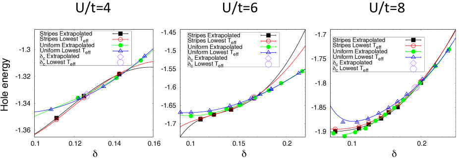
Figure 8: Determination of the critical doping where the transition between the uniform phase and the stripe phase occurs with lower energy at small doping. The empty big dots (tilted squares) represent the transition points corresponding to the best variational estimates (extrapolated to zero temperature ones) at the lowest effective temperatures $T_{\mathrm{eff}}$

As in HF theory, away from the commensurate dopings $1/W$, an insulating phase covering a continuum of different dopings can be constructed by appropriately joining such commensurate solutions, i.e. a doping $2/13$ with insulating properties can be easily obtained by alternating a $W=7$ stripe with a $W=6$ one. This is actually the case in a $26\times 12$ cluster, within VAFQMC, namely the $6+7+6+7$ alternating stripe length solution has an energy slightly lower than the corresponding one $6+6+7+7$, thus satisfying the HF rule stated at the end of the previous section. This phase, competing with the uniform $d_{x^{2}-y^{2}}$ BCS one, has a full charge gap in $H_{MF}(\bm{\alpha_{0}})$, a property that cannot be changed by a small $\tau-$projection. Moreover no coexistence of stripe and BCS order was found within VAFQMC.

In summary, according to Fig. 8, it is possible to conclude that an insulating stripe phase acquires an energy lower than the corresponding uniform phase already at quite large doping around $\delta\simeq 20\%$. Nevertheless, it is important to remark that the uniform phase has a very good energy, competing with the lowest possible ones. Indeed in Fig. 4 the uniform $d-wave$ phase looses only a tiny energy (less than $0.001t$ per site at the lowest $T_{\mathrm{eff}}$) vs the nonuniform stripe phases. Interestingly just around the doping $\delta=1/8$ equally spaced stripes with length $W<1/\delta$ appear lowest in energy, as can be seen in Fig. 9, where the energy of such metallic (at least within the mean-field Hamiltonian $H_{MF}(\bm{\alpha_{0}})$) stripes are compared with the commensurate insulating ones (black lines). For instance the $W=9$ stripe at doping around $1/13$ (i.e. a metallic stripe with $W<1/\delta$) has an hole energy more than $0.01t$ below the corresponding insulating stripe with $W=13$, a huge gain that can be hardly explained by artifacts of the approximations (finite $T_{\mathrm{eff}}$ and/or finite clusters). In this plot we also see that phase separation (a minimum of the hole energy) cannot be excluded for doping $\delta\lesssim 5\%$ but the results strongly depend on the extrapolation and requires therefore more accuracy to be settled. By judging from the extrapolated values it is plausible to expect a similar flat behavior of the energy per hole at low doping as in the corresponding HF plot (Fig.7a). However, within HF, a metallic solution with $W<1/\delta$ was never found to have the lowest energy at low doping, again in agreement with Ref.Schulz, 1990.

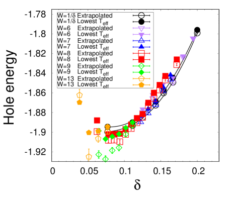
Figure 9: Hole energy at $U/t=8$ for equally spaced stripes of different length $W$ as a function of the doping $\delta$, by considering clusters of dimension larger than $12\times 2W$, namely enough to have negligible finite size effects. For doping around $\delta\simeq{1\over 8}$ stripes with length $W<{1\over\delta}$ become energetically stable and acquire metallic character as the mean-field bands defining the variational wave function used in this work are only partially filled. The commensurate stripe results with $\delta=1/W$ are connected by black lines.

In the following it is worth to discuss rather extensively the main result of this work, namely that, at large doping the stripe melts and a small but sizable superconducting d-wave order clearly remains within the present approach, in the sense that the energy is lowered in the thermodynamic limit by breaking the $U(1)$ global symmetry related to number of particle conservation. This is because both the mean-field Hamiltonians $H_{MF}(\bm{\alpha_{0}})$ and $H_{MF}(\bm{\alpha})$ clearly support a broken symmetry solution of this type when $\Delta_{x^{2}-y^{2}}>0$ in Eq. LABEL:hmf. Indeed, in Fig. 10 the superconducting gap $\Delta_{x^{2}-y^{2}}$ parameter, corresponding to $H_{MF}(\bm{\alpha_{0}})$, is displayed for $U/t=8$ as a function of the doping.

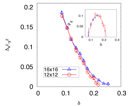
Figure 10: $\Delta_{x^{2}-y^{2}}$ BCS pairing variational parameter in the mean-field Hamiltonian $H_{MF}(\bm{\alpha_{0}})$ (see Eq. LABEL:hmf) defining the spatially uniform variational ansatz of Eq. (1), as a function of the doping $\delta$ for the lowest $T_{\mathrm{eff}}$ and largest clusters considered. Inset: value of the corresponding BCS order parameter evaluated with the $T_{\mathrm{eff}}\to 0$ linear extrapolation of the pairing-paring correlations at distance $L/2$. The error bars include also uncertainty in this extrapolation.

When the $\Delta_{x^{2}-y^{2}}$ is large there are negligible size effects. However when it approaches zero, a long slowly decaying tail shows evident size effects. Indeed with the largest affordable sizes it is possible that the calculated critical doping $\delta_{c}$ above which a symmetric phase is stable indicates only a sharp crossover region separating a phase with sizable strong coupling superconductivity from another phase with very small order parameter, compatible with an exponentially small pairing of the Kohn-Luttinger typeHlubina (1999); Deng et al. (2015). Indeed, within weak coupling theory, the $d-wave$ superconducting phase should remain stable up to $\simeq 40\%$ doping, a doping much larger than the one detected in the present work.

As shown in Fig. 11, within this approach, the critical doping characterizing a strong coupling superconductivity (i.e. a non negligible pairing) can be identified because for $\mu\leq\mu_{c}$ the energy clearly improves by increasing the value of $\Delta_{x^{2}-y^{2}}$ even when starting from a negligible value, representing the symmetric Fermi liquid ground state. Nevertheless there may be non negligible size effects as shown for $U/t=8$, especially considering the difficulty to locate the end of a long tiny tail of the order parameter, as discussed before. Moreover, for smaller $U$ these size effects are expected even larger, but much larger cluster simulations are prohibitive at present. For this reason for $U/t=2$ ($U/t=4$) a much larger mesh for the TABC was used with $64\times 64$ ($32\times 32$) different twists in the BZ, instead of the smaller $16\times 16$ grid used for $U/t=8$ and $U/t=6$. In a mean-field calculation a $64\times 64$ TABC grid in a $16\times 16$ square lattice corresponds to a $1024\times 1024$ cluster with PBC, large enough to probe even a very tiny but non negligible gap parameter $\Delta_{x^{2}-y^{2}}$. Remarkably, at $U/t=2$ no evidence of such a tiny value of the order parameter is found in all relevant doping region, as can be clearly seen in Fig. 11.

Figure 11: $\Delta_{x^{2}-y^{2}}$ BCS pairing variational parameter in the mean-field Hamiltonian $H_{MF}(\bm{\alpha_{0}})$ defining the spatially uniform variational ansatz of Eq. (1), as a function of the energy optimization iterations at the lowest $T_{\mathrm{eff}}$ (i.e. largest $\tau t=4,2.6,1.73,1.3$ for $U/t=2,4,6,8$, respectively) and $16\times 16$ cluster. For all cases the initial wave function was prepared with $\Delta_{x^{2}-y^{2}}=0$ defining the Fermi liquid state. Then this parameter was set to a small value and the iterative stochastic optimization was started. In these calculations, in order to reduce at most the stochastic bias, at each iteration a quite large number ($>3\times 10^{5}$) of samples for evaluating energy derivatives was used, in a way that they are sensitive to very small energy differences $<10^{-5}t$. Optimization of the grand potential $\Omega$ at fixed chemical potential $\mu$ was employed in all cases shown. The corresponding doping was estimated by ${\partial\Omega\over\partial\mu}=-(1-\delta)N_{s}$ using the data for $\Omega$ reported in the supplementary material SI extrapolated to the $T_{\mathrm{eff}}\to 0$ limit. These estimates are consistent with the direct evaluation of the doping $\delta=1-{\langle\psi_{\tau}|\hat{N}|\psi_{\tau}\rangle\over N_{s}\langle\psi_{\tau}|\psi_{\tau}\rangle}$ at the lowest $T_{\mathrm{eff}}$ within half the confidence doping interval reported for each $U/t\neq 2$.

This small but relevant strong coupling region where d-wave superconductivity appears to be stable in the Hubbard model is in agreement with the old findings by cluster dynamical mean-field theoryMaier et al. (2005), though it is located at a slight higher doping, namely at 10% the stripe should be stable also for $U/t=4$. Moreover it is worth mentioning a recent VMC calculationDarmawan et al. (2018) employed at $U/t=10$ and density matrix embedding theory(DMET)Zheng and Chan (2016) supporting also the stability of a $d-$wave superconductivity in a small doping region. On the other hand the proposed phase diagram is also in agreement with the claimQin et al. (2020) of absence of $d-$wave superconductivity in the 2D Hubbard model, because in this work the authors refer mainly to doping $1/8$, where no BCS pairing was found also in this work. The final phase diagram is therefore reported in Fig. 12.

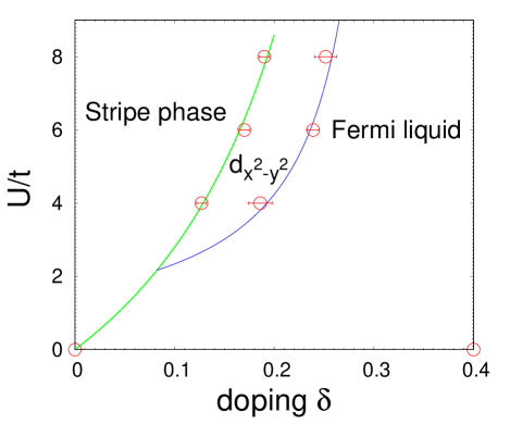
Figure 12: Phase diagram of the Hubbard model by VAFQMC. Blue and green continuous lines are simple interpolations of the transition points (open circles, $\delta=19\%-25.2\%,17\%-23.9\%,12.7\%-18.6\%$ for $U/t=8,6,4$, respectively). The blue line is also determined by the condition that for $U/t=2$ no BCS pairing has been detected, while the green line by the one that the incommensurate spin order cannot show up at non zero doping for $U\to 0$Schulz (1990). In the stripe phase there may be a transition between an insulating stripe and a small doping metallic stripe, as suggested by Fig. 9 for $U/t=8$. In this transition the mean-field VAFQMC Hamiltonian $H_{MF}(\bm{\alpha_{0}})$ has a finite gap (bands are completely filled) or a vanishing one, respectively.

VII Conclusions

In this work the VAFQMC method, able to exploit the power of the auxiliary field technique combined with the simplicity and generality of the standard variational quantum Monte Carlo method, has been introduced. By combining these two successful approaches to strongly correlated systems, it is possible to estimate the evolution of the phase diagram of a lattice model, by improving systematically the accuracy of the correlation term, starting from the HF approximation. This is achieved by lowering an effective temperature $T_{\mathrm{eff}}$ up to a value that turns out to be low enough to provide very accurate variational energies of the Hubbard model in the thermodynamic limit, while remaining far from any sign problem instability, so far affecting most fermion quantum Monte Carlo techniques. Within the assumption that the tiny energy gain between different broken symmetry phases of the model can be sorted out by a careful optimization of a mean-field ansatz in presence of an accurate enough correlation term, the phase diagrams obtained in this way should be considered reliable, at least for the phases studied.

It is clear that the above assumption is very important as, for instance in the Hubbard model, we have estimated an energy per site error of about $2\times 10^{-3}t$ ($4\times 10^{-4}t$) at $U/t=8$ ($U/t=4$), while energy differences of the various phases at the lowest $T_{\mathrm{eff}}$ considered can be even more than an order of magnitude smaller. This is not a difficulty of the present method, providing state of the art variational energies (see supplementary information for detailed benchmark results), but clarifies once more the enormous challenge of the electron correlation problem in numerical calculations. For instance on such clusters it is basically impossible to distinguish an unbroken symmetric metallic phase from a $d-$wave superconducting one with small $\Delta_{x^{2}-y^{2}}$ gap parameter, by judging merely on correlation functions (e.g. pairing correlations), and the above assumption provides a much more sensitive criterium for occurrence of broken symmetry phenomena. Relying on the above assumption, dramatically helps numerical techniques, such as VAFQMC, able to work with boundary conditions fulfilling the symmetries of $H$, that may be possibly broken in the thermodynamic limit.

In any case, the present work provides rigorous and accurate upper bounds of the ground state energies of the Hubbard model for several $U/t$ and doping values well converged in the thermodynamic limit (see supplementary information), that can be useful in future works on this important subject and/or for benchmarking new computational, theoretical or experimental techniques. The fact that extrapolated energies do not depend much on the ansatz adopted (all extrapolated energies agree within $0.001t$ per site) implies that energetic properties are settled within a reasonable accuracy. However, in order to get the right order without assuming it in the initial mean-field ansatz, much larger projection times are required (see for instance Fig.4 where two completely different phases differ in energy by less than $0.001t$ per site), that are at present not possible.

In this study many different mean-field solutions have been attempted with several different initializations of parameters, including also broken time reversal solutionsLee et al. (2006) and different modulations of stripes and pairing. In all cases the smooth convergence of the energy as a function of $T_{\mathrm{eff}}$ has been verified. This is not only important for achieving reasonable extrapolations but especially for excluding being trapped in spurious local minima, that is a limitation of any non linear optimization technique. The phase diagram presented here in Fig.12 shows the phases so far determined with the lowest possible variational energies among the chosen ansatzs.

An important progress in this study is the control of finite size effects within VAFQMC. The conventional approach is to attempt exact calculations (usually very hard if not impossible) at finite number of sites $N_{s}$ and try to extrapolate to ${1\over N_{s}}\to 0$. Within VAFQMC it is much simpler and indeed possible to extrapolate only in the effective temperature $T_{\mathrm{eff}}\to 0$ limit the finite $T_{\mathrm{eff}}\gtrsim t/2$ results. To this purpose it is enough to perform $N_{s}\gtrsim 100$ calculations because they are already very close to the ${1\over N_{s}}\to 0$ limit, thanks to the very effective twisted average boundary condition method.

The results shown in this work are weakly affected by the sign problem. In general the average sign, appearing for instance in the denominator of Eq. (16), should decay exponentially to zero both with $1/T_{\mathrm{eff}}$ and $N_{s}$, yielding prohibitive statistical errors. However for $T_{\mathrm{eff}}$ large enough (i.e. the ones used here) the exponential decay in $N_{s}$ of the average sign is very weak, due to a stability property of the adopted auxiliary field technique, that was discovered several years agoSORELLA (1991). Hence much larger clusters could be safely simulated, that is very promising considering also that the ones reported here are not far from the state of the art simulations not vexed by the ”sign problem”.

In this work a large stripe phase in the Hubbard model exists as an effective way to expel the holes from a clean antiferromagnet. In this way genuine phase separation does not occur in the Hubbard model as a result of a very weak repulsive coupling between stripes at large distance. In practice, at small doping, the energy per hole is almost constant, namely the inverse charge compressibility is vanishingly small, in agreement with the phase separation scenarioEmery et al. (1990) and some previous numerical calculationsCosentini et al. (1998); Chang and Zhang (2008); Sorella (2015).

An important outcome of the present work is that a sizable superconducting phase is present in the Hubbard model with a non negligible order parameter only in the strong coupling regime. For instance for $U/t=2$ no evidence of $d_{x^{2}-y^{2}}$ BCS order was probed and the maximum $\Delta_{x^{2}-y^{2}}\simeq 0.02t$ was obtained with the largest $U/t=8$ considered at about $20\%$ doping. The critical doping $\delta_{c}$ separating the metal from the $d-$wave superconductor turns out to be much smaller than the one obtained with weak coupling analysisHlubina (1999); Deng et al. (2015) and the question is how to reconcile the weak and the strong coupling limits. In principle, as suggested by the results in Fig. 10, a small tail with very weak BCS pairing could distinguish a strong coupling phase with sizable pairing and a weak coupling phase with a sharp crossover (and not a transition) clearly separating the two regimes.

The main features of cuprate superconductivity can be explained with the Hubbard model, but quantitatively there remain several unsolved issues. First, the stripes are completely filled by holes and do not match the half filled ones detected experimentallyTranquada et al. (1995). Second, the $d-$wave superconductivity is sizable but still far to explain $T_{c}\simeq 100K$ because the gap function, that is growing when approaching the Mott insulating phase at zero doping (see Fig.10), is limited by the phase transition to the stripe phase.

VAFQMC has been developed to study properties of strongly correlated systems in the thermodynamic limit. Obviously this method applies also to finite systems for obtaining the best ground state estimates with the largest possible projection time $\tau$. However for finite systems, the symmetry is never broken, and a more accurate wave function should be used by restoring the symmetry with appropriate projection operatorsShi et al. (2014); Tahara and Imada (2008), an improvement that can be done and should be worth doing for this particular purpose. Moreover, several new applications and extensions are possible within VAFQMC. The WF $|\psi_{\tau}\rangle$ can be further generalized to more realistic Hamiltonians, including for instance long range Coulomb interaction or electron-phonon coupling. The finite effective temperature $T_{\mathrm{eff}}$ here defined for a variational wave function is the key to obtain very accurate results well converged in the thermodynamic limit, a feature that could be possibly generalized to several other computational techniques, from tensor networks to machine learning variational wave functions.

Appendix A Finite effective temperature $T_{\mathrm{eff}}$ corrections for the infinite volume ground state projection

Given a $\tau/2$-projected trial function $|\psi_{\tau}\rangle=\exp(-H\tau/2)|\psi_{MF}\rangle$ the pseudo partition function,

$$Z(\tau)=\langle\psi_{\tau}|\psi_{\tau}\rangle=\langle\psi_{MF}|\exp(-\tau H)|\psi_{MF}\rangle,$$ (22)

is considered in the following, namely with an effective temperature $T_{\mathrm{eff}}={1\over\tau}$ fixed when the infinite volume thermodynamic limit is employed. Here the particular case of the Heisenberg model $H=J\sum\limits_{<ij>}\vec{S}_{i}\cdot\vec{S}_{j}$ and $|\psi_{MF}\rangle=|{\rm N\acute{e}el}\rangle$ is studied, but, due to universality, the results should apply to any model, where a classical symmetry, parametrized by a $M-$dimensional real vector is broken. In particular it holds for the wave function of Eq.(1) in the main text, for collinear magnetic order $M=3$ (apply also for the stripe phase) and superconducting $M=2$ one. In the Heisenberg model, in $D$ dimensions, the low energy limit can be studied by introducing coherent states $\vec{n}$ with $|\vec{n}|^{2}=1$ and, by integrating over one of the two sublatticesParola (1989), it follows that:

$$Z=\int d\left[\vec{n}\right]_{0,\tau}\exp\left\{-{1\over 2}\int\limits_{0}^{\tau}dt\int dr^{D}\left[\chi|\partial_{t}\vec{n}|^{2}+\Upsilon\sum\limits_{\nu=1}^{D}|\partial_{\nu}\vec{n}|^{2}\right]\right\}$$ (23)

with the notations given in Ref.Fisher, 1989, where $\Upsilon$ is the spin-wave stiffness and $\chi$ is the transverse susceptibility. In the case of the pseudo partition function of Eq.(23) the following boundary conditions for the $M-$ component field $\vec{n}(\vec{r},t)$ hold:

$$\vec{n}(\vec{r},0)=\vec{n}(\vec{r},\tau)=(1,0,\cdots,0)$$ (24)

because the field at the boundary of the time interval is constrained to have the value of the trial function $|\psi_{MF}\rangle$, a Néel state with the antiferromagnetic order along the x-axis.

Due to the above boundary conditions, the $M-1$ component vector $\vec{\Pi}$, describing the field fluctuations, and defined by:

$$\vec{n}(\vec{r},t)=(1-{|\vec{\Pi}(\vec{r},t)|^{2}\over 2},\vec{\Pi}(\vec{r},t))+o(\Pi^{2})$$ (25)

acquires the following Fourier decomposition:

$$\vec{\Pi}(\vec{r},t)=\sqrt{2\over\tau V}\sum\limits_{n>0,\vec{q}}\vec{\Pi}_{n,\vec{q}}\sin(\omega_{n}t)\exp(i\vec{q}\cdot\vec{r})$$ (26)

where $\vec{q}={2\pi\over L}(n_{x},n_{y},\cdots)$ are the momenta allowed by the periodic boundary conditions, whereas $\omega_{n}={\pi n\over\tau}$ for integers $n>0$, in order to satisfy that the field vanishes at $t=0$ and $t=\tau$. Notice that, in the usual partition function at finite temperature $T={1\over\tau}$ the quantization of the frequencies $\omega_{n}={2\pi n\over\tau}$ (also non positive integers allowed) is slightly different and the calculations can be easily generalized, but they have already been reported in previous worksFisher (1989); Hasenfratz and Niedermayer (1993); Hofmann (2010). Therefore we just mention in the following the standard finite temperature case, in order to check the results derived in this section.

With the above definition, the pseudo partition function acquires a Gaussian form at leading order, valid in the ordered phase:

$$Z = \int\left[d\vec{\Pi}\right]\exp\left\{-{1\over 2}\sum\limits_{n,\vec{q}}(\chi\omega_{n}^{2}+\Upsilon|\vec{q}|^{2})|\vec{\Pi}_{n,\vec{q}}|^{2}\right\}$$ (27)

$$\propto \exp\{-{M-1\over 2}\sum\limits_{n,\vec{q}}\ln(\chi\omega_{n}^{2}+\Upsilon|\vec{q}|^{2})\}$$

On the other hand the average propagator over these Gaussian fluctuations can be readily evaluated:

$$\langle\Pi^{\nu}_{n,\vec{q}}\Pi^{\nu}_{n,-\vec{q}}\rangle={1\over\chi\omega_{n}^{2}+\Upsilon|\vec{q}|^{2}}$$ (28)

where $\nu=1,2,\cdots M-1$ labels the components of the vector $\vec{\Pi}.$

A.1 Energy and order parameter

The expectation value of the energy $E(\tau)$ over the state $|\psi_{\tau}\rangle=\exp(-H\tau/2)|\psi_{MF}\rangle$ can be written as:

$$E(\tau)=-\partial_{\tau}\ln Z$$ (29)

Since $E(\tau)$ in the expression (27), depends on $\tau$ only by means of $\omega_{n}$, it follows that:

$$E(\tau)=-{(M-1)\over\tau}\sum_{n>0,\vec{q}}{\chi\omega_{n}^{2}\over\chi\omega_{n}^{2}+\Upsilon|\vec{q}|^{2}}$$ (30)

On the other hand the local magnetization:

$$m(\tau)={\langle\psi_{\tau}|{1\over V}\int d\vec{r}^{D}(1-{\Pi(\vec{r},\tau/2)^{2}\over 2})|\psi_{\tau}\rangle\over\langle\psi_{\tau}|\psi_{\tau}\rangle}$$ (31)

can be easily evaluated by the knowledge of the propagator in Eq.(28) and the definition of the component in the ordered x-direction in Eq.(25):

$$m(\tau)=1-{(M-1)\over V\tau}\sum\limits_{n>0,\vec{q}}{\sin({\omega_{n}\tau\over 2})^{2}\over\chi\omega_{n}^{2}+\Upsilon|\vec{q}|^{2}}$$ (32)

A.2 Evaluation

As in any field theory the above expressions diverge without introducing infinite counter terms. In the expression of the energy one can subtract and add one in the integrand, whereas in the correction of the magnetic moment it is enough to deal with particular care the $q=0$ mode (this mode may be also avoided by using twisted boundary conditions):

$$E/V = {M-1\over\tau V}\sum\limits_{n>0,\vec{q}}{\Upsilon|\vec{q}|^{2}\over\chi\omega_{n}^{2}+\Upsilon|\vec{q}|^{2}}-{M-1\over\tau V}\sum\limits_{n>0,\vec{q}}1$$

$$m(\tau) = 1-{(M-1)\over V\tau}\sum\limits_{n>0,\vec{q}}{\sin({\omega_{n}\tau\over 2})^{2}\over\chi\omega_{n}^{2}+\Upsilon|\vec{q}|^{2}}$$ (33)

The infinite RHS term in the energy corresponds to an infinite shift of the ground state energy, a typical feature of quantum field theories, as this shift becomes finite by introducing a cutoff, implicitly present in any physical model.

In order to evaluate the above expressions it is useful to consider the following sum:

$$\sum_{n}{1\over z+n}=\pi\cot(\pi z)$$ (34)

that is valid for any complex number $z$. In particular for $z={1\over 2}+iy$ we obtain:

$$\sum_{n}{1\over{1\over 2}+iy+n}=-i\pi\tanh(\pi y)$$ (35)

whereas for $z=iy$ we get:

$$\sum_{n}{1\over iy+n}=-i\pi\coth(\pi y)$$ (36)

Defining the velocity of the Goldstone’s modes $c=\sqrt{\Upsilon\over\chi}$, the sum over $n$ is extended to $-\infty\leq n\leq\infty$, using the even dependence on $n$ and taking into account the extra $n=0$ contribution in the definition of $\epsilon_{0}$. In this way, by using Eq. 36 for evaluating the infinite sums the universal finite size corrections are given by:

$$E/V = {M-1\over 2\tau V}\sum\limits_{n=-\infty}^{\infty}\sum\limits_{\vec{q}}{i\sqrt{\Upsilon}|q|\over 2}\left[{1\over\sqrt{\chi}\omega_{n}+i\sqrt{\Upsilon}|q|}\right.$$ (37)

$$- \left.{1\over\sqrt{\chi}\omega_{n}-i\sqrt{\Upsilon}|q|}\right]-{M-1\over 2\tau V}\sum\limits_{n=-\infty}^{\infty}\sum\limits_{\vec{q}}1$$

$$= \epsilon_{0}+{(M-1)c\over 2V}\sum\limits_{\vec{q}}|q|(\coth(c|q|\tau)-1)$$

where $\epsilon_{0}$ is the ”infinite” ground state energy corrected for the zero point harmonic energy $\epsilon_{0}={M-1\over 2V}\sum\limits_{\vec{q}}c|q|-{M-1\over\tau 2V}\sum\limits_{n=-\infty}^{\infty}\sum\limits_{\vec{q}}1$, a divergent expression depending on the cutoff but not on the boundary conditions (i.e. it is the same divergent term appearing in Ref.Fisher, 1989, by using the trace). In the thermodynamic limit and fixed $\tau$ the convergent contribution can be worked out, by replacing sums over momenta with integrals (i.e. ${1\over V}\sum\limits_{q}\to\int({dq\over 2\pi})^{D}$), and changing the momentum scale $\vec{q}\to c\tau\vec{q}$, so that:

$$E/V=\epsilon_{0}+{(M-1)\over 2c^{D}}f_{e}T_{\mathrm{eff}}^{D+1}$$ (38)

where $f_{e}$ is a dimensional dependent constant defined by:

$$f_{e}=\int({dq\over 2\pi})^{D}|q|(\coth(|q|)-1)$$ (39)

that is clearly a convergent integral for any dimension $D\geq 1$ because $\coth(|q|)$ converges to one exponentially for large $|q|$. The values of $f_{e}$ are therefore $\pi\over 12$, $\zeta(3)\over 4\pi$ ($\zeta(3)=1.20205690316$) and $\pi^{2}\over 240$ in $D=1$, $D=2$ and $D=3$, respectively. In $D=1$ the coefficient $f_{e}$ has not to be taken for granted, since no true long range order is possible (see later), but the qualitative behavior of the correction $\simeq T_{\mathrm{eff}}^{2}$ should hold as it is consistent with the corresponding finite temperature correction derived in $D=1$ for the 1D-Hubbard model by means of the Bethe AnsatzTakahashi (1972).

Thus, in the thermodynamic limit, the finite $\tau$ corrections to the energy depend only on the universal constant $f_{e}$, the number of components $M$ of the order parameter, and the velocity $c$ of the gapless Goldstone modes. In D=2 the finite temperature corrections to the internal energy at infinite volume have been determined in Ref.Hasenfratz and Niedermayer (1993). For this purpose we have repeated the same type of calculation and get that, taking into account the different boundary condition for the field (PBC in time for the trace $\tau=\beta=1/T$):

$$E(T)/V-\epsilon_{0} = {(M-1)c\over 2}\int({dq\over 2\pi})^{D}|q|(\coth({c|q|\beta\over 2})-1)$$ (40)

$$= {(M-1)c\over 2({c\over 2T})^{D+1}}f_{e}$$

that is consistent with the previous calculation reported in D=2, i.e.Hasenfratz and Niedermayer (1993):

$$E(T)/V-\epsilon_{0}=(M-1){\zeta(3)\over c^{2}\pi}T^{3}$$ (41)

On the other hand, for the magnetic order parameter, by noticing that $\sin({\omega_{n}\tau\over 2})^{2}=1$ for $n=2\nu+1$ and zero otherwise, the sum has to be evaluated for odd integer frequencies $\omega_{\nu}={\pi(2\nu+1)\over\tau}$. For this purpose the sum $\sum\limits_{\nu=0}^{\infty}{1\over\chi\omega_{\nu}^{2}+\Upsilon|\vec{q}|^{2}}$ is extended to ${1\over 2}\sum\limits_{\nu=-\infty}^{\infty}{1\over\chi\omega_{\nu}^{2}+\Upsilon|\vec{q}|^{2}}$ because $\omega_{\nu}=-\omega_{-(\nu+1)}$ for $\nu<0$. Therefore by applying Eq. 35 for evaluating the following infinite sums, one obtains:

$$\Delta m(\tau) = -{M-1\over 2V\tau}\sum\limits_{\nu,\vec{q}}{i\over 2\sqrt{\Upsilon}|q|}\left[{1\over{\sqrt{\chi}\pi\over\tau}(2\nu+1)+i\sqrt{\Upsilon}|q|}\right.$$

$$- \left.{1\over{\sqrt{\chi}\pi\over\tau}(2\nu+1)-i\sqrt{\Upsilon}|q|}\right]$$

$$= -{M-1\over 4V\sqrt{\chi\Upsilon}}\sum\limits_{\vec{q}\neq 0}{(\tanh(c|q|\tau/2)-1)\over|q|}-\Delta m_{0}$$

$$= -\Delta m_{0}-{M-1\over 4\sqrt{\chi\Upsilon}c^{D-1}}f_{m}T_{\mathrm{eff}}^{D-1}$$

where $\Delta m_{0}={(M-1)\tau\over 8V\chi}+{M-1\over 4\sqrt{\chi\Upsilon}V}\sum\limits_{\vec{q}\neq 0}{1\over|q|}$ (the first term in $\Delta m_{0}$ is the $q=0$ contribution in Eq. 33 that is convergent for finite $\tau$) and the dimensional dependent constant $f_{m}$ is defined by:

$$f_{m}=\int({dq\over 2\pi})^{D}(\tanh({|q|\over 2})-1)/|q|$$ (43)

that converges in $D>1$. The values of $f_{m}$ are therefore $-{\ln(2)\over\pi}$ and $-{1\over 12}$ for $D=2$ and $D=3$, respectively.

Thus, in the thermodynamic limit the finite $T_{\mathrm{eff}}$ corrections to the antiferromagnetic order parameter depend on the universal constant $f_{m}$, the number of components $M$ of the order parameter, the velocity $c$ and the stiffness $\Upsilon$ of the gapless Goldstone modes.

Notice that the expression above for $f_{m}$ converges in $D=2$. Instead if periodic boundary conditions in $\tau$ are assumed for the field $\vec{\Pi}(x,t)$, corresponding to the standard finite temperature calculation at $\beta=\tau$, by repeating the same steps, it follows that: $\Delta m(\tau)=-{M-1\over 2V\sqrt{\chi\Upsilon}}\sum\limits_{q\neq 0}{\coth(c|q|\tau/2)\over|q|}$ which blows up for $D\leq 2$, thus recovering the Mermin-Wagner theoremMermin and Wagner (1966): no finite $m$ is possible at finite temperature for $D\leq 2$. The advantage of using the projection technique is therefore evident especially in $D=2$ for the study of broken symmetry phases, that are possible, for continuous symmetries, only at zero temperature.

When using finite cylinders with even $L_{y}$ all the above results obtained for $D=1$ apply because the $y$ momentum $q_{y}={2\pi n_{y}\over L_{y}}$ is quantized with $n_{y}=0,1,\cdots,L_{y}-1$ and only the $q_{y}=0$ momentum value provides power law corrections in $1/\tau$ to energy and correlation functions (if converging). This is because all the other contributions acquire a finite $\sim{1\over L_{y}}$ gap and converge much faster.

Appendix B Convexity of the energy as a function density

One can divide a large system $A+B$ in two regions $A$ and $B$ containing a macroscopic number of sites $L_{A}$ and $L_{B}$ and electrons $N_{A}$ and $N_{B}$, respectively. Then, by defining $E_{A+B}$ the energy of the total system, $E_{A}$ and $E_{B}$ the ones of the corresponding parts, $\rho={N_{A}+N_{B}\over L_{A}+L_{B}}=p\rho_{1}+(1-p)\rho_{2}$, $\rho_{1}={N_{A}\over L_{A}}$, $\rho_{2}={N_{B}\over L_{B}}$, $p={L_{A}\over L_{A}+L_{B}}$, $e(\rho_{1})=E_{A}/L_{A}$ and $e(\rho_{2})=E_{B}/L_{B}$ converged in the thermodynamic limit because the two parts are macroscopic, then $e(\rho)={E_{A+B}\over L_{A}+L_{B}}\leq{E_{A}+E_{B}\over L_{A}+L_{B}}=pe(\rho_{1})+(1-p)e(\rho_{2})$ follows because one can neglect in the thermodynamic limit the surface term contribution to the energy separating the region A from the region B. This is because, by assumption, the model is short range as the hopping term connects only nearest neighbor sites and the interaction $U$ is on site. The final inequality:

$$e(\rho)\leq pe(\rho_{1})+(1-p)e(\rho_{2})$$ (44)

therefore holds for arbitrary densities $\rho_{1}\leq\rho\leq\rho_{2}$ and implies, the convexity property of the function $e(\rho)$ in the thermodynamic limit. Whenever phase separation occurs between two densities $\rho_{1}$ and $\rho_{2}$ the inequality 44 turns to a strict equality, namely $e(\rho)$ is a linear function of the density because $p={\rho-\rho_{2}\over\rho_{1}-\rho_{2}}$, so that in particular the energy per hole in Eq. 20 is constant for $\delta\leq\delta_{c}$.

References

- Kohn and Sham (1965) W. Kohn and L. J. Sham, Phys. Rev. 140, A1133 (1965).
- White (1992) S. R. White, Phys. Rev. Lett. 69, 2863 (1992).
- Schollwöck (2005) U. Schollwöck, Rev. Mod. Phys. 77, 259 (2005).
- Orús (2014) R. Orús, Annals of Physics 349, 117 (2014).
- Verstraete et al. (2004) F. Verstraete, D. Porras, and J. I. Cirac, Phys. Rev. Lett. 93, 227205 (2004).
- Schuch et al. (2011) N. Schuch, D. Pérez-García, and I. Cirac, Phys. Rev. B 84, 165139 (2011).
- Sorella et al. (1989) S. Sorella, S. Baroni, R. Car, and M. Parrinello, Europhysics Letters (EPL) 8, 663 (1989).
- Corney and Drummond (2004) J. F. Corney and P. D. Drummond, Phys. Rev. Lett. 93, 260401 (2004).
- Efetov et al. (2009) K. B. Efetov, C. Pépin, and H. Meier, Phys. Rev. Lett. 103, 186403 (2009).
- Booth et al. (2013) G. H. Booth, A. Grüneis, G. Kresse, and A. Alavi, Nature 493, 365 (2013).
- Dobrautz et al. (2019) W. Dobrautz, H. Luo, and A. Alavi, Phys. Rev. B 99, 075119 (2019).
- Yao et al. (2020) Y. Yao, E. Giner, J. Li, J. Toulouse, and C. J. Umrigar, The Journal of Chemical Physics 153, 124117 (2020), https://doi.org/10.1063/5.0018577 .
- Carleo and Troyer (2017) G. Carleo and M. Troyer, Science 355, 602 (2017), https://science.sciencemag.org/content/355/6325/602.full.pdf .
- Carleo et al. (2019) G. Carleo, I. Cirac, K. Cranmer, L. Daudet, M. Schuld, N. Tishby, L. Vogt-Maranto, and L. Zdeborová, Rev. Mod. Phys. 91, 045002 (2019).
- Lieb and Wu (1968) E. H. Lieb and F. Y. Wu, Phys. Rev. Lett. 20, 1445 (1968).
- Kitaev (2006) A. Kitaev, Annals of Physics 321, 2 (2006), january Special Issue.
- Mazurenko et al. (2017) A. Mazurenko, C. S. Chiu, G. Ji, M. F. Parsons, M. Kanász-Nagy, R. Schmidt, F. Grusdt, E. Demler, D. Greif, and M. Greiner, Nature 545, 462 (2017).
- Hirsch (1985) J. E. Hirsch, Phys. Rev. B 31, 4403 (1985).
- Seki and Sorella (2019) K. Seki and S. Sorella, Phys. Rev. B 99, 144407 (2019).
- LeBlanc et al. (2015) J. P. F. LeBlanc, A. E. Antipov, F. Becca, I. W. Bulik, G. K.-L. Chan, C.-M. Chung, Y. Deng, M. Ferrero, T. M. Henderson, C. A. Jiménez-Hoyos, E. Kozik, X.-W. Liu, A. J. Millis, N. V. Prokof’ev, M. Qin, G. E. Scuseria, H. Shi, B. V. Svistunov, L. F. Tocchio, I. S. Tupitsyn, S. R. White, S. Zhang, B.-X. Zheng, Z. Zhu, and E. Gull (Simons Collaboration on the Many-Electron Problem), Phys. Rev. X 5, 041041 (2015).
- Zheng et al. (2017) B.-X. Zheng, C.-M. Chung, P. Corboz, G. Ehlers, M.-P. Qin, R. M. Noack, H. Shi, S. R. White, S. Zhang, and G. K.-L. Chan, Science 358, 1155 (2017), https://science.sciencemag.org/content/358/6367/1155.full.pdf .
- Zhang et al. (1997) S. Zhang, J. Carlson, and J. E. Gubernatis, Phys. Rev. Lett. 78, 4486 (1997).
- Maier et al. (2005) T. A. Maier, M. Jarrell, T. C. Schulthess, P. R. C. Kent, and J. B. White, Phys. Rev. Lett. 95, 237001 (2005).
- Deng et al. (2015) Y. Deng, E. Kozik, N. V. Prokofev, and B. V. Svistunov, EPL (Europhysics Letters) 110, 57001 (2015).
- Qin et al. (2020) M. Qin, C.-M. Chung, H. Shi, E. Vitali, C. Hubig, U. Schollwöck, S. R. White, and S. Zhang (Simons Collaboration on the Many-Electron Problem), Phys. Rev. X 10, 031016 (2020).
- Sorella et al. (2002) S. Sorella, G. B. Martins, F. Becca, C. Gazza, L. Capriotti, A. Parola, and E. Dagotto, Phys. Rev. Lett. 88, 117002 (2002).
- Note (1) Considering the same unit the order parameter was consistent with the previous calculation obtained by VMCSorella et al. (2002) at around 15% doping.
- Becca and Sorella (2017) F. Becca and S. Sorella, Quantum Monte Carlo approaches for correlated systems (Cambridge University Press, 2017).
- Umrigar et al. (2007) C. J. Umrigar, J. Toulouse, C. Filippi, S. Sorella, and R. G. Hennig, Phys. Rev. Lett. 98, 110201 (2007).
- Sorella et al. (1989) S. Sorella, S. Baroni, R. Car, and M. Parrinello, EPL (Europhysics Letters) 8, 663 (1989).
- White et al. (1989) S. R. White, D. J. Scalapino, R. L. Sugar, E. Y. Loh, J. E. Gubernatis, and R. T. Scalettar, Phys. Rev. B 40, 506 (1989).
- Loh et al. (1990) E. Y. Loh, J. E. Gubernatis, R. T. Scalettar, S. R. White, D. J. Scalapino, and R. L. Sugar, Phys. Rev. B 41, 9301 (1990).
- Eichenberger and Baeriswyl (2007) D. Eichenberger and D. Baeriswyl, Phys. Rev. B 76, 180504(R) (2007).
- Yanagisawa et al. (1998) T. Yanagisawa, S. Koike, and K. Yamaji, Journal of the Physical Society of Japan 67, 3867 (1998), https://doi.org/10.1143/JPSJ.67.3867 .
- Yanagisawa (2016) T. Yanagisawa, Journal of the Physical Society of Japan 85, 114707 (2016), https://doi.org/10.7566/JPSJ.85.114707 .
- Beach et al. (2019) M. J. S. Beach, R. G. Melko, T. Grover, and T. H. Hsieh, Phys. Rev. B 100, 094434 (2019).
- Wecker et al. (2015) D. Wecker, M. B. Hastings, and M. Troyer, Phys. Rev. A 92, 042303 (2015).
- Sorella (1998) S. Sorella, Phys. Rev. Lett. 80, 4558 (1998).
- Amari (1998) S. Amari, Neural Computation 10, 251 (1998).
- Fisher (1989) D. S. Fisher, Phys. Rev. B 39, 11783 (1989).
- Hasenfratz and Niedermayer (1993) P. Hasenfratz and F. Niedermayer, Zeitschrift für Physik B Condensed Matter 92, 91 (1993).
- Hofmann (2010) C. P. Hofmann, Phys. Rev. B 81, 014416 (2010).
- Lin et al. (2001) C. Lin, F. H. Zong, and D. M. Ceperley, Phys. Rev. E 64, 016702 (2001).
- Gros (1996) C. Gros, Phys. Rev. B 53, 6865 (1996).
- Karakuzu et al. (2018) S. Karakuzu, K. Seki, and S. Sorella, Phys. Rev. B 98, 075156 (2018).
- Note (2) From this point of view VAFQMC is not different from standard AFQMC or VMC and the expectation value of any operator, not only , can be computed without particular effort.Becca and Sorella (2017).
- Note (3) The numerator and the denominator of Eq. (14) are both real after summations over and because they correspond to the RHS of Eq. (10) and the Hamiltonian is Hermitian. Therefore the real part can be moved inside the summations of Eq. (14) with no approximation.
- Griewank (2000) A. Griewank, Evaluating Derivatives: Principles and Techniques of Algo- rithmic Differentiation (Frontiers in Applied Mathematics, Philadelphia, 2000).
- Griewank (2012) A. Griewank, Documenta Math. Extra Volume, 389 (2012).
- Sorella and Capriotti (2010) S. Sorella and L. Capriotti, The Journal of Chemical Physics 133, 234111 (2010), https://doi.org/10.1063/1.3516208 .
- Liao et al. (2019) H.-J. Liao, J.-G. Liu, L. Wang, and T. Xiang, Phys. Rev. X 9, 031041 (2019).
- Note (4) Convergence in the thermodynamic limit has also been verified by comparing with the cluster within an error of about .
- Note (5) Obviosuly possible DMRG calculations with should provide energies better than the VAFQMC reported ones. So this remark does not imply that VAFQMC provides in general variational energies better than DMRG.
- Tocchio et al. (2019) L. F. Tocchio, A. Montorsi, and F. Becca, SciPost Phys. 7, 21 (2019).
- Corboz et al. (2018) P. Corboz, P. Czarnik, G. Kapteijns, and L. Tagliacozzo, Phys. Rev. X 8, 031031 (2018).
- Chung and White (2018) C.-M. Chung and S. R. White, private communication (2018).
- Corboz (2017) P. Corboz, private communication (2017).
- Schulz (1990) H. J. Schulz, Phys. Rev. Lett. 64, 1445 (1990).
- Xu et al. (2011) J. Xu, C.-C. Chang, E. J. Walter, and S. Zhang, Journal of physics. Condensed matter : an Institute of Physics journal 23 50, 505601 (2011).
- Emery et al. (1990) V. J. Emery, S. A. Kivelson, and H. Q. Lin, Phys. Rev. Lett. 64, 475 (1990).
- Note (6) Spin-up and spin-down bands are degenerate due to the reflection symmetry around any stripe, namely a vertical axis with maximum hole density, see Fig. 2. This transformation changes the spin direction of the antiferromagnetic field, namely the spin-up with the spin-down HF Hamiltonian, that therefore have the same spectrum of eigenvalues.
- Hlubina (1999) R. Hlubina, Phys. Rev. B 59, 9600 (1999).
- Darmawan et al. (2018) A. S. Darmawan, Y. Nomura, Y. Yamaji, and M. Imada, Phys. Rev. B 98, 205132 (2018).
- Zheng and Chan (2016) B.-X. Zheng and G. K.-L. Chan, Phys. Rev. B 93, 035126 (2016).
- Lee et al. (2006) P. A. Lee, N. Nagaosa, and X.-G. Wen, Rev. Mod. Phys. 78, 17 (2006).
- SORELLA (1991) S. SORELLA, International Journal of Modern Physics B 05, 937 (1991), https://doi.org/10.1142/S0217979291000493 .
- Cosentini et al. (1998) A. C. Cosentini, M. Capone, L. Guidoni, and G. B. Bachelet, Phys. Rev. B 58, R14685 (1998).
- Chang and Zhang (2008) C.-C. Chang and S. Zhang, Phys. Rev. B 78, 165101 (2008).
- Sorella (2015) S. Sorella, Phys. Rev. B 91, 241116(R) (2015).
- Tranquada et al. (1995) J. M. Tranquada, B. J. Sternlieb, J. D. Axe, Y. Nakamura, and S. Uchida, Nature 375, 561 (1995).
- Shi et al. (2014) H. Shi, C. A. Jiménez-Hoyos, R. Rodríguez-Guzmán, G. E. Scuseria, and S. Zhang, Phys. Rev. B 89, 125129 (2014).
- Tahara and Imada (2008) D. Tahara and M. Imada, Journal of the Physical Society of Japan 77, 114701 (2008), https://doi.org/10.1143/JPSJ.77.114701 .
- Parola (1989) A. Parola, Phys. Rev. B 40, 7109 (1989).
- Takahashi (1972) M. Takahashi, Progress of Theoretical Physics 47, 69 (1972), https://academic.oup.com/ptp/article-pdf/47/1/69/5305353/47-1-69.pdf .
- Mermin and Wagner (1966) N. D. Mermin and H. Wagner, Phys. Rev. Lett. 17, 1133 (1966).