Mind the Gap
when Conditioning Amortised Inference
in Sequential Latent-Variable Models
Abstract
Amortised inference enables scalable learning of sequential latent-variable models (LVMs) with the evidence lower bound (ELBO). In this setting, variational posteriors are often only partially conditioned. While the true posteriors depend, e. g., on the entire sequence of observations, approximate posteriors are only informed by past observations. This mimics the Bayesian filter—a mixture of smoothing posteriors. Yet, we show that the ELBO objective forces partially-conditioned amortised posteriors to approximate products of smoothing posteriors instead. Consequently, the learned generative model is compromised. We demonstrate these theoretical findings in three scenarios: traffic flow, handwritten digits, and aerial vehicle dynamics. Using fully-conditioned approximate posteriors, performance improves in terms of generative modelling and multi-step prediction.
1 Introduction
Variational inference has paved the way towards learning deep latent-variable models (LVMs): maximising the evidence lower bound (ELBO) approximates maximum likelihood learning (Jordan et al., 1999; Beal, 2003; MacKay, 2003). An efficient variant is amortised variational inference where the approximate posteriors are represented by a deep neural network, the inference network (Hinton et al., 1995). It produces the parameters of the variational distribution for each observation by a single forward pass—in contrast to classical variational inference with a full optimisation process per sample. The framework of variational auto-encoders (Kingma & Welling, 2014; Rezende et al., 2014) adds the reparameterisation trick for low-variance gradient estimates of the inference network. Learning of deep generative models is hence both tractable and flexible, as all its parts can be represented by neural networks and fit by stochastic gradient descent.
The quality of the solution is largely determined by how well the true posterior is approximated: the gap between the ELBO and the log marginal likelihood is the KL divergence from the approximate to the true posterior. Recent works have proposed ways of closing this gap, suggesting tighter alternatives to the ELBO (Burda et al., 2016; Mnih & Rezende, 2016) or more expressive variational posteriors (Rezende & Mohamed, 2015; Mescheder et al., 2017). Cremer et al. (2018) provide an analysis of this gap, splitting it in two. The approximation gap is caused by restricting the approximate posterior to a specific parametric form, the variational family. The amortisation gap comes from the inference network failing to produce the optimal parameters within the family.
In this work, we address a previously unstudied aspect of amortised posterior approximations: successful approximate posterior design is not merely about picking a parametric form of a probability density. It is also about carefully deciding which conditions to feed into the inference network. This is a particular problem in sequential LVMs, where it is common practice to feed only a restricted set of inputs into the inference network: not conditioning on latent variables from other time steps can vastly improve efficiency (Bayer & Osendorfer, 2014; Lai et al., 2019). Further, leaving out observations from the future structurally mimics the Bayesian filter, useful for state estimation in the control of partially observable systems (Karl et al., 2017b; Hafner et al., 2019; Lee et al., 2020).
We analyse the emerging conditioning gap and the resulting suboptimality for sequential amortised inference models. If the variational posterior is only partially conditioned, all those posteriors equal w. r. t. included conditions but different on the excluded ones will need to share an approximate posterior. The result is a suboptimal compromise over many different true posteriors which cannot be mitigated by improving variational family or inference network capacity. We empirically show its effects in an extensive study on three real-world data sets on the common use case of variational state-space models.
2 Amortised Variational Inference
2.1 Variational Auto-Encoders
Consider the task of fitting the parameters of a latent-variable model to a target distribution by maximum likelihood:
| (1) |
In the case of variational auto-encoders (VAEs), the prior distribution is often simple, such as a standard Gaussian. The likelihood on the other hand is mostly represented by a deep neural network producing the likelihood parameters as a function of .
The log marginal likelihood contains a challenging integral within a logarithm. The maximisation of eq. 1 is thus generally intractable. Yet, for a single sample the log marginal likelihood can be bounded from below by the evidence lower bound (ELBO):
| (2) | ||||
where a surrogate distribution , the variational posterior, is introduced. The bound is tighter the better approximates . The gap vanishes with the posterior KL divergence in eq. 2.
Typically, the target distribution is given by a finite data set . In classical variational inference, equally many variational posteriors are determined by direct optimisation. For instance, each Gaussian is represented by its mean and standard deviation . The set of all possible distributions of that parametric form is called the variational family . Learning the generative model parameters can then be performed by an empirical risk minimisation approach, where the average negative ELBO over a data set is minimised:
The situation is different for VAEs. The parameters of the approximate posterior for a specific sample are produced by another deep neural network, the inference network . Instead of directly optimising for sample-wise parameters, a global set of weights for the inference network is found by stochastic gradient-descent of the expected negative ELBO:
This approach tends to scale more gracefully to large data sets.
The Sequential Case
The posterior of a sequential latent-variable model
of observations and latents , with , factorises as
| (3) |
The posterior KL divergence is a sum of step-wise divergences (Cover & Thomas, 2006):
| (4) |
where we have left out the conditions of for now. This decomposition allows us to focus on the non-sequential case in our theoretical analysis, even though the phenomenon most commonly occurs with sequential LVMs.
2.2 The Approximation and Amortisation Gaps
The ELBO and the log marginal likelihood are separated by the posterior Kullback-Leibler divergence , cf. eq. 2. If the optimal member of the variational family is not equal to the true posterior, or , then
so that the ELBO is strictly lower than the log marginal likelihood—the approximation gap.
Using an inference network we must expect that even the optimal variational posterior within the variational family is not found in general. The gap widens:
This phenomenon was first discussed by Cremer et al. (2018). The additional gap
is called the amortisation gap.
The two gaps represent two distinct suboptimality cases when training VAEs. The former is caused by the choice of variational family, the latter by the success of the amortised search for a good candidate .
3 Partial Conditioning of Inference Networks
| Model | ||
| STORN (Bayer & Osendorfer, 2014) | ||
| VRNN (Chung et al., 2015) | ||
| DKF (Krishnan et al., 2015) | (exper.) | |
| DKS (Krishnan et al., 2017) | – | |
| DVBF (Karl et al., 2017a) | ||
| Planet (Hafner et al., 2019) | ||
| SLAC (Lee et al., 2020) |
VAEs add an additional consideration to approximate posterior design compared to classical variational inference: the choice of inputs to the inference networks. Instead of feeding the entire observation , one can choose to feed a strict subset . This is common practice in many sequential variants of the VAE, cf. table 1, typically motivated by efficiency or downstream applications. The discrepancy between inference models inputs and the true posterior conditions has been acknowledged before, e. g. by Krishnan et al. (2017), where they investigate different variants. Their analysis does not go beyond quantitative empirical comparisons. In the following, we show that such design choices lead to a distinct third cause of inference suboptimality, the conditioning gap.
3.1 Minimising Expected KL Divergences Yields Products of Posteriors
The root cause is that all observations that share the same included conditions but differ in the excluded conditions must now share the same approximate posterior by design. This shared approximate posterior optimizes the expected KL divergence
| (5) |
w. r. t. the missing conditions . By rearranging (cf. section A.1 for details)
where denotes a normalising constant, we see that the shared optimal approximate posterior is
Interestingly, this expression bears superficial similarity with the true partially-conditioned posterior
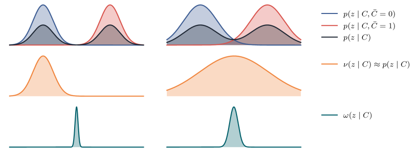
To understand the difference, consider a uniform discrete for the sake of the argument. In this case, the expectation is an average over all missing conditions. The true posterior is then a mixture distribution of all plausible full posteriors . The optimal approximate posterior, because of the logarithm inside the sum, is a product of plausible full posteriors. Such distributions occur e. g. in products of experts (Hinton, 2002) or Gaussian sensor fusion (Murphy, 2012). Products behave differently from mixtures: an intuition due to Welling (2007) is that a factor in a product can single-handedly “veto” a sample, while each term in a mixture can only “pass” it.
This intuition is highlighted in fig. 1. We can see that is located between the modes and sharply peaked. It shares almost no mass with both the posteriors and the marginal posterior. The approximate marginal posterior on the other hand either covers one or two modes, depending on the width of the two full posteriors–-a much more reasonable approximation.
In fact, will only coincide with either or in the the extreme case when , cf. section A.2, which implies statistical independence of and given .
Notice how the suboptimality of assumed neither a particular variational family, nor imperfect amortisation— is the analytically optimal shared posterior. Both approximation and amortisation gap would only additionally affect the KL divergence inside the expectation in eq. 5. As such, the inference suboptimality described here can occur even if those vanish. We call
| (6) |
the conditioning gap, which in contrast to approximation and amortisation gap can only be defined as an expectation w. r. t. .
Notice further that the effects described here assumed the KL divergence, a natural choice due to its duality with the ELBO (cf. eq. 2). To what extent alternative divergences (Ranganath et al., 2014; Li & Turner, 2016) exhibit similar or more favourable behaviour is left to future research.
Learning Generative Models with Partially-Conditioned Posteriors
We find that the optimal partially-conditioned posterior will not correspond to desirable posteriors such as or , even assuming that the variational family could represent them. This also affects learning the generative model. A simple variational calculus argument (section A.3) reveals that, when trained with partially-conditioned approximate posteriors, maximum-likelihood models and ELBO-optimal models are generally not the same. In fact, they coincide only in the restricted cases where . As seen before this is the case if and only if .
3.2 Learning a Univariate Gaussian
It is worth highlighting the results of this section in a minimal scalar linear Gaussian example. The target distribution is . We assume the latent variable model
with free parameter . This implies
With , we recover the target distribution with posterior . Next, we introduce the variational approximation . With the only condition missing, this is a deliberately extreme case of partial conditioning where and . Notice that the true posterior is a member of the variational family, i. e., no approximation gap. We maximise the expected ELBO
i. e., all observations from share the same approximation . One can show that
We immediately see that is neither equal to nor to . Less obvious is that the variance of the optimal solution is much smaller than that of both and . This is a consequence of the product of the expert compromise discussed earlier: the (renormalised) product of Gaussian densities will always have lower variance than either of the factors. This simple example highlights how poor shared posterior approximations can become.
Further, inserting back into the expected ELBO and optimising for reveals that the maximum likelihood model parameter is not optimal. In other words, does not optimise the expected ELBO in —despite being the maximum likelihood model.
3.3 Extension to the Sequential Case
The conditioning gap may arise in each of the terms of eq. 4 if is partially conditioned. Yet, it is common to leave out future observations, e. g. . To the best of our knowledge, in the literature only sequential applications of VAEs are potentially affected by the conditioning gap. Still, sequential latent-variable models with amortised under-conditioned posteriors have been applied success fully to, e. g., density estimation, anomaly detection, and sequential decision making (Bayer & Osendorfer, 2014; Soelch et al., 2016; Hafner et al., 2019). This may seem at odds with the previous results. The gap is not severe in all cases. Let us emphasize two “safe” cases where the gap vanishes because is approximately true. First, where the partially- and the fully-conditioned posterior correspond to the prior transition, i. e.
This is for example the case for deterministic dynamics where the transition is a single point mass. Second, the case where the observations are sufficient to explain the latent state, i. e.
A common case are systems with perfect state information.
Several studies have shown that performance gains of fully-conditioned over partially-conditioned approaches are negligible (Fraccaro et al., 2016; Maddison et al., 2017; Buesing et al., 2018). We conjecture that the mentioned “safe” cases are overrepresented in the studied data sets. For example, environments for reinforcement learning such as the gym or MuJoCo environments (Todorov et al., 2012; Brockman et al., 2016) feature deterministic dynamics. We will address a broader variety of cases in section 5.
4 Related Work
The bias of the ELBO has been studied numerous times (Nowozin, 2018; Huang & Courville, 2019). A remarkable study by Turner & Sahani (2011) contains a series of carefully designed experiments showing how different forms of assumptions on the approximate posterior let different qualities of the solutions emerge. This study predates the introduction of amortised inference (Kingma & Welling, 2014; Rezende et al., 2014) however. Cremer et al. (2018) identify two gaps arising in the context of VAEs: the approximation gap, i. e. inference error resulting from the true posterior not being a member of variational family; and the amortisation gap, i. e. imperfect inference due to an amortised inference procedure, e. g. a single neural network call. Both gaps occur per sample and are independent of the problems in section 3.
Applying stochastic gradient variational Bayes (Kingma & Welling, 2014; Rezende et al., 2014) to sequential models was pioneered by Bayer & Osendorfer (2014); Fabius et al. (2015); Chung et al. (2015). The inclusion of state-space assumptions was henceforth demonstrated by Archer et al. (2015); Krishnan et al. (2015; 2017); Karl et al. (2017a); Fraccaro et al. (2016; 2017); Becker-Ehmck et al. (2019). Specific applications to various domains followed, such as video prediction (Denton & Fergus, 2018), tracking (Kosiorek et al., 2018; Hsieh et al., 2018; Akhundov et al., 2019) or simultaneous localisation and mapping (Mirchev et al., 2019). Notable performance in model-based sequential decision making has also been achieved by Gregor et al. (2019); Hafner et al. (2019); Lee et al. (2020); Karl et al. (2017b); Becker-Ehmck et al. (2020). The overall benefit of latent sequential variables was however questioned by Lai et al. (2019). The performance of sequential latent-variable models in comparison to auto-regressive models was studied, arriving at the conclusion that the added stochasticity does not increase, but even decreases performance. We want to point out that their empirical study is restricted to the setting where , see the appendix of their work. We conjecture that such assumptions lead to a collapse of the model where the latent variables merely help to explain the data local in time, i. e. intra-step correlations.
A related field is that of missing-value imputation. Here, tasks have increasingly been solved with probabilistic models (Ledig et al., 2017; Ivanov et al., 2019). The difference to our work is the explicit nature of the missing conditions. Missing conditions are typically directly considered by learning instead of and appropriate changes to the loss functions.
5 Study: Variational State-Space Models
We study the implications of section 3 for the case of variational state-space models (VSSMs). We deliberately avoid the cases of deterministic dynamics and systems with perfect state information: unmanned aerial vehicle (UAV) trajectories with imperfect state information in section 5.2, a sequential version of the MNIST data set section 5.3 and traffic flow in section 5.4. The reason is that the gap is absent in these cases, see section 3.3. In all cases, we not only report the ELBO, but conduct qualitative evaluations as well. We start out with describing the employed model in section 5.1.
5.1 Variational State-Space Models
The two Markov assumptions that every observation only depends on the current state and every state only depends on the previous state and condition lead to the following generative model:
where are additional conditions from the data set (such as control signals) and . We consider three different conditionings of the inference model
partial with , semi with , and full with . We call the sneak peek, inspired by Karl et al. (2017a). See appendix B for more details.
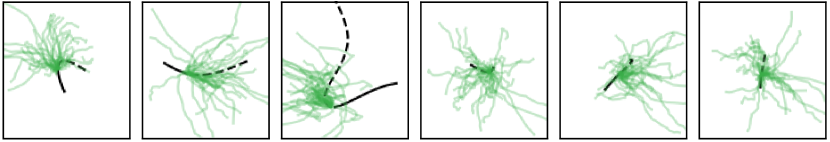
5.2 UAV Trajectories from the Blackbird Data Set
We apply semi- and fully-conditioned VSSMs to UAV modelling (Antonini et al., 2018). By discarding the rotational information, we create a system with imperfect state information, cf. section 3.3. Each observation is the location of an unmanned aerial vehicle (UAV) in a fixed global frame. The conditions , consist of IMU readings, rotor speeds, and pulse-width modulation. The emission model was implemented as a Gaussian with fixed, hand-picked standard deviations, where the mean corresponds to the first three state dimensions (cf. (Akhundov et al., 2019)): . We leave out the partially-conditioned case, as it cannot infer the higher-order derivatives necessary for rigid-body dynamics. A sneak peek of for the semi-conditioned model is theoretically sufficient to infer those moments. See appendix C for details.
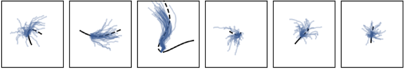
Fully-conditioned models outperform semi-conditioned ones on the test set ELBO, as can be seen in table 2(a). We evaluated the models on prefix-sampling, i. e. the predictive performance of . To restrict the analysis to the found parameters of the generative model only, we inferred the filter distribution using a bootstrap particle filter (Sarkka, 2013). By not using the respective approximate posteriors, we ensure fairness between the different models. Samples from the predictive distribution were obtained via ancestral sampling of the generative model. Representative samples are shown in fig. 4. We performed a posterior-predictive check for both models, where we compare the densities of the final observations obtained from prefix sampling in fig. 2. Both evaluations qualitatively illustrate that the predictions of the fully-conditioned approach concentrate more around the true values. In particular the partially-conditioned model struggles more with long-term prediction.
| UAV | Traffic Flow | |||
| val | test | val | test | |
| partial | - | - | ||
| semi | ||||
| full | ||||
| Distribution | Log-Likelihood | KL |
| data | - | |
| partial | ||
| full | ||
| vhp + rewo | - | |
| iwae (L=2) | - |
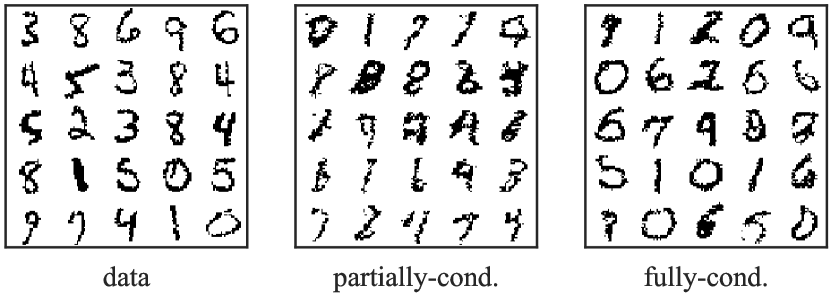
5.3 Row-Wise MNIST
We transformed the MNIST data set into a sequential data set by considering one row in the image plane per time step, from top to bottom. This results in stochastic dynamics: similiar initial rows can result in a 3, 8, 9 or 0, future rows are very informative (cf. section 3.3). Before all experiments, each pixel was binarised by sampling from a Bernoulli with a rate in proportional to the corresponding pixel intensity.
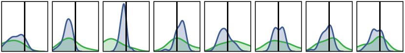
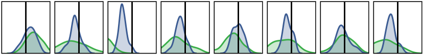
The setup was identical to that of section 5.2, except that a Bernoulli likelihood parameterised by a feed-forward neural network was used: . No conditions and a short sneak-peek () were used. The fully-conditioned model outperforms the partially-conditioned by a large margin, placing it significantly closer to state-of-the-art performance, see table 2(b). This is supported by samples from the model, see fig. 3. Cf. appendix D for details.
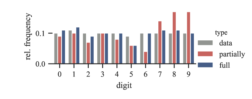
For qualitative evaluation, we used a state-of-the-art classifier111https://github.com/keras-team/keras/blob/2.4.0/examples/mnist_cnn.py to categorise 10,000 samples from each of the models. If the data distribution is learned well, we expect the classifier to behave similarly on both data and generative samples, i. e. yield uniformly distributed class predictions. We report KL-divergences from the uniform distribution of the class prediction distributions in table 2(b). A bar plot of the induced class distributions can be found in fig. 3. Only the fully-conditioned model is able to nearly capture a uniform distribution.
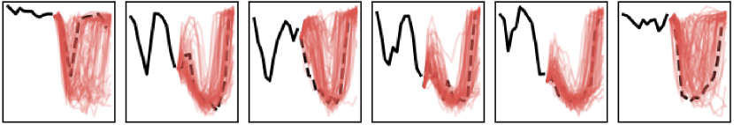
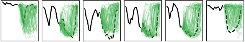
5.4 Traffic Flow
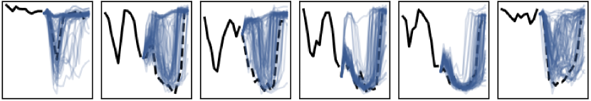
We consider the Seattle loop data set (Cui et al., 2019; 2020) of average speed measurements of cars at 323 locations on motorways near Seattle, from which we selected a single one (42). The dynamics of this system are highly stochastic, which is of special interest for our study, cf. section 3.3. Even though all days start out very similar, traffic jams can emerge suddenly. In this scenario the emission model was a feed-forward network conditioned on the whole latent state, i. e. . We compare partially-, semi- () and fully-conditioned models. See appendix E for details. The results are shown in table 2(a). While the fully-conditioned posterior emerges as the best choice on the validation set, the semi-conditioned and the fully-conditioned one are on par on the test set. We suspect that the sneak peek is sufficient to fully capture a sensible initial state approximation.
We performed a qualitative evaluation of this scenario as well in the form of prefix sampling. Given the first observations, the task is to predict the remaining ones for the day, compare section 5.2. We show the results in fig. 4. The fully-conditioned model clearly shows more concentrated yet multi-modal predictive distributions. The partially-condition model concentrates too much, and the semi-conditioned one too little.
| UAV | Traffic Flow | |
| partial | - |
|
| semi |
|
|
| full |
|
|
6 Discussion & Conclusion
We studied the effect of leaving out conditions of amortised posteriors, presenting strong theoretical findings and empirical evidence that it can impair maximum likelihood solutions and inference. Our work helps with approximate posterior design and provides intuitions for when full conditioning is necessary. We advocate that partially-conditioned approximate inference models should be used with caution in downstream tasks as they may not be adequate for the task, e. g., replacing a Bayesian filter. In general, we recommend conditioning inference models conforming to the true posterior.
References
- Akhundov et al. (2019) Adnan Akhundov, Maximilian Soelch, Justin Bayer, and Patrick van der Smagt. Variational Tracking and Prediction with Generative Disentangled State-Space Models. arXiv:1910.06205 [cs, stat], October 2019. URL http://arxiv.org/abs/1910.06205.
- Antonini et al. (2018) Amado Antonini, Winter Guerra, Varun Murali, Thomas Sayre-McCord, and Sertac Karaman. The blackbird dataset: A large-scale dataset for UAV perception in aggressive flight. In Jing Xiao, Torsten Kröger, and Oussama Khatib (eds.), Proceedings of the 2018 International Symposium on Experimental Robotics, ISER 2018, Buenos Aires, Argentina, November 5-8, 2018, volume 11 of Springer Proceedings in Advanced Robotics, pp. 130–139. Springer, 2018. doi: 10.1007/978-3-030-33950-0““˙12. URL https://doi.org/10.1007/978-3-030-33950-0_12.
- Archer et al. (2015) Evan Archer, Il Memming Park, Lars Buesing, John Cunningham, and Liam Paninski. Black box variational inference for state space models. arXiv:1511.07367 [stat], November 2015. URL http://arxiv.org/abs/1511.07367.
- Bayer & Osendorfer (2014) Justin Bayer and Christian Osendorfer. Learning Stochastic Recurrent Networks. arXiv:1411.7610 [cs, stat], November 2014. URL http://arxiv.org/abs/1411.7610.
- Beal (2003) Matthew J. Beal. Variational Algorithms for Approximate Bayesian Inference. PhD thesis, University College London, UK, 2003. URL http://ethos.bl.uk/OrderDetails.do?uin=uk.bl.ethos.404387.
- Becker-Ehmck et al. (2019) Philip Becker-Ehmck, Jan Peters, and Patrick van der Smagt. Switching Linear Dynamics for Variational Bayes Filtering. In Kamalika Chaudhuri and Ruslan Salakhutdinov (eds.), Proceedings of the 36th International Conference on Machine Learning, volume 97 of Proceedings of Machine Learning Research, pp. 553–562, Long Beach, California, USA, 2019. PMLR. URL http://proceedings.mlr.press/v97/becker-ehmck19a.html.
- Becker-Ehmck et al. (2020) Philip Becker-Ehmck, Maximilian Karl, Jan Peters, and Patrick van der Smagt. Learning to Fly via Deep Model-Based Reinforcement Learning. arXiv:2003.08876 [cs, stat], August 2020. URL http://arxiv.org/abs/2003.08876.
- Bottou (2010) Léon Bottou. Large-scale machine learning with stochastic gradient descent. In Yves Lechevallier and Gilbert Saporta (eds.), 19th International Conference on Computational Statistics, COMPSTAT 2010, Paris, France, August 22-27, 2010 - Keynote, Invited and Contributed Papers, pp. 177–186. Physica-Verlag, 2010. doi: 10.1007/978-3-7908-2604-3““˙16. URL https://doi.org/10.1007/978-3-7908-2604-3_16.
- Brockman et al. (2016) Greg Brockman, Vicki Cheung, Ludwig Pettersson, Jonas Schneider, John Schulman, Jie Tang, and Wojciech Zaremba. OpenAI Gym. arXiv:1606.01540 [cs], June 2016. URL http://arxiv.org/abs/1606.01540.
- Buesing et al. (2018) Lars Buesing, Theophane Weber, Sebastien Racaniere, S. M. Ali Eslami, Danilo Rezende, David P. Reichert, Fabio Viola, Frederic Besse, Karol Gregor, Demis Hassabis, and Daan Wierstra. Learning and Querying Fast Generative Models for Reinforcement Learning. arXiv:1802.03006 [cs], February 2018. URL http://arxiv.org/abs/1802.03006.
- Burda et al. (2016) Yuri Burda, Roger B. Grosse, and Ruslan Salakhutdinov. Importance weighted autoencoders. In Yoshua Bengio and Yann LeCun (eds.), 4th International Conference on Learning Representations, ICLR 2016, San Juan, Puerto Rico, May 2-4, 2016, Conference Track Proceedings, 2016. URL http://arxiv.org/abs/1509.00519.
- Chung et al. (2015) Junyoung Chung, Kyle Kastner, Laurent Dinh, Kratarth Goel, Aaron C. Courville, and Yoshua Bengio. A Recurrent Latent Variable Model for Sequential Data. In Corinna Cortes, Neil D. Lawrence, Daniel D. Lee, Masashi Sugiyama, and Roman Garnett (eds.), Advances in Neural Information Processing Systems 28: Annual Conference on Neural Information Processing Systems 2015, December 7-12, 2015, Montreal, Quebec, Canada, pp. 2980–2988, 2015. URL http://papers.nips.cc/paper/5653-a-recurrent-latent-variable-model-for-sequential-data.
- Cover & Thomas (2006) Thomas M. Cover and Joy A. Thomas. Elements of Information Theory. Wiley Series in Telecommunications and Signal Processing. Wiley-Interscience, USA, 2006. ISBN 978-0-471-24195-9.
- Cremer et al. (2018) Chris Cremer, Xuechen Li, and David Duvenaud. Inference suboptimality in variational autoencoders. In Jennifer G. Dy and Andreas Krause (eds.), Proceedings of the 35th International Conference on Machine Learning, ICML 2018, Stockholmsmässan, Stockholm, Sweden, July 10-15, 2018, volume 80 of Proceedings of Machine Learning Research, pp. 1086–1094. PMLR, 2018. URL http://proceedings.mlr.press/v80/cremer18a.html.
- Cui et al. (2019) Zhiyong Cui, Ruimin Ke, Ziyuan Pu, and Yinhai Wang. Deep Bidirectional and Unidirectional LSTM Recurrent Neural Network for Network-wide Traffic Speed Prediction. arXiv:1801.02143 [cs], November 2019. URL http://arxiv.org/abs/1801.02143.
- Cui et al. (2020) Zhiyong Cui, Kristian Henrickson, Ruimin Ke, and Yinhai Wang. Traffic graph convolutional recurrent neural network: A deep learning framework for network-scale traffic learning and forecasting. IEEE Transactions on Intelligent Transportation Systems, 21(11):4883–4894, 2020. doi: 10.1109/TITS.2019.2950416. URL https://doi.org/10.1109/TITS.2019.2950416.
- Denton & Fergus (2018) Emily Denton and Rob Fergus. Stochastic video generation with a learned prior. In Jennifer G. Dy and Andreas Krause (eds.), Proceedings of the 35th International Conference on Machine Learning, ICML 2018, Stockholmsmässan, Stockholm, Sweden, July 10-15, 2018, volume 80 of Proceedings of Machine Learning Research, pp. 1182–1191. PMLR, 2018. URL http://proceedings.mlr.press/v80/denton18a.html.
- van Erven & Harremoës (2014) Tim van Erven and Peter Harremoës. Rényi divergence and kullback-leibler divergence. IEEE Transactions on Information Theory, 60(7):3797–3820, 2014. doi: 10.1109/TIT.2014.2320500. URL https://doi.org/10.1109/TIT.2014.2320500.
- Fabius et al. (2015) Otto Fabius, Joost R. van Amersfoort, and Diederik P. Kingma. Variational recurrent auto-encoders. In Yoshua Bengio and Yann LeCun (eds.), 3rd International Conference on Learning Representations, ICLR 2015, San Diego, CA, USA, May 7-9, 2015, Workshop Track Proceedings, 2015. URL http://arxiv.org/abs/1412.6581.
- Fraccaro et al. (2016) Marco Fraccaro, Søren Kaae Sønderby, Ulrich Paquet, and Ole Winther. Sequential neural models with stochastic layers. In Daniel D. Lee, Masashi Sugiyama, Ulrike von Luxburg, Isabelle Guyon, and Roman Garnett (eds.), Advances in Neural Information Processing Systems 29: Annual Conference on Neural Information Processing Systems 2016, December 5-10, 2016, Barcelona, Spain, pp. 2199–2207, 2016. URL https://proceedings.neurips.cc/paper/2016/hash/208e43f0e45c4c78cafadb83d2888cb6-Abstract.html.
- Fraccaro et al. (2017) Marco Fraccaro, Simon Kamronn, Ulrich Paquet, and Ole Winther. A disentangled recognition and nonlinear dynamics model for unsupervised learning. In Isabelle Guyon, Ulrike von Luxburg, Samy Bengio, Hanna M. Wallach, Rob Fergus, S. V. N. Vishwanathan, and Roman Garnett (eds.), Advances in Neural Information Processing Systems 30: Annual Conference on Neural Information Processing Systems 2017, December 4-9, 2017, Long Beach, CA, USA, pp. 3601–3610, 2017. URL https://proceedings.neurips.cc/paper/2017/hash/7b7a53e239400a13bd6be6c91c4f6c4e-Abstract.html.
- Gelfand & Fomin (2003) I. M. Gelfand and S. V. Fomin. Calculus of Variations. Dover Publications Inc., Mineola, N.Y, March 2003. ISBN 978-0-486-41448-5.
- Gregor et al. (2019) Karol Gregor, George Papamakarios, Frederic Besse, Lars Buesing, and Theophane Weber. Temporal difference variational auto-encoder. In 7th International Conference on Learning Representations, ICLR 2019, New Orleans, LA, USA, May 6-9, 2019. OpenReview.net, 2019. URL https://openreview.net/forum?id=S1x4ghC9tQ.
- Hafner et al. (2019) Danijar Hafner, Timothy P. Lillicrap, Ian Fischer, Ruben Villegas, David Ha, Honglak Lee, and James Davidson. Learning latent dynamics for planning from pixels. In Kamalika Chaudhuri and Ruslan Salakhutdinov (eds.), Proceedings of the 36th International Conference on Machine Learning, ICML 2019, 9-15 June 2019, Long Beach, California, USA, volume 97 of Proceedings of Machine Learning Research, pp. 2555–2565. PMLR, 2019. URL http://proceedings.mlr.press/v97/hafner19a.html.
- Hinton et al. (1995) G. E. Hinton, P. Dayan, B. J. Frey, and R. M. Neal. The ”wake-sleep” algorithm for unsupervised neural networks. Science, 268(5214):1158–1161, May 1995. ISSN 0036-8075, 1095-9203. doi: 10.1126/science.7761831. URL https://science.sciencemag.org/content/268/5214/1158.
- Hinton (2002) Geoffrey E. Hinton. Training Products of Experts by Minimizing Contrastive Divergence. Neural Computation, 14(8):1771–1800, August 2002. ISSN 0899-7667. doi: 10.1162/089976602760128018. URL https://www.mitpressjournals.org/doi/10.1162/089976602760128018.
- Hoffman et al. (2013) Matthew D. Hoffman, David M. Blei, Chong Wang, and John Paisley. Stochastic Variational Inference. Journal of Machine Learning Research, 14(4):1303–1347, 2013. ISSN 1533-7928. URL http://jmlr.org/papers/v14/hoffman13a.html.
- Hsieh et al. (2018) Jun-Ting Hsieh, Bingbin Liu, De-An Huang, Fei-Fei Li, and Juan Carlos Niebles. Learning to decompose and disentangle representations for video prediction. In Samy Bengio, Hanna M. Wallach, Hugo Larochelle, Kristen Grauman, Nicolò Cesa-Bianchi, and Roman Garnett (eds.), Advances in Neural Information Processing Systems 31: Annual Conference on Neural Information Processing Systems 2018, NeurIPS 2018, December 3-8, 2018, Montréal, Canada, pp. 515–524, 2018. URL https://proceedings.neurips.cc/paper/2018/hash/496e05e1aea0a9c4655800e8a7b9ea28-Abstract.html.
- Huang & Courville (2019) Chin-Wei Huang and Aaron Courville. Note on the bias and variance of variational inference. arXiv:1906.03708 [cs, stat], June 2019. URL http://arxiv.org/abs/1906.03708.
- Ivanov et al. (2019) Oleg Ivanov, Michael Figurnov, and Dmitry P. Vetrov. Variational autoencoder with arbitrary conditioning. In 7th International Conference on Learning Representations, ICLR 2019, New Orleans, LA, USA, May 6-9, 2019. OpenReview.net, 2019. URL https://openreview.net/forum?id=SyxtJh0qYm.
- Jordan et al. (1999) Michael I. Jordan, Zoubin Ghahramani, Tommi S. Jaakkola, and Lawrence K. Saul. An introduction to variational methods for graphical models. Machine Learning, 37(2):183–233, 1999. doi: 10.1023/A:1007665907178. URL https://doi.org/10.1023/A:1007665907178.
- Karl et al. (2017a) Maximilian Karl, Maximilian Soelch, Justin Bayer, and Patrick van der Smagt. Deep Variational Bayes Filters: Unsupervised Learning of State Space Models from Raw Data. In 5th International Conference on Learning Representations, ICLR 2017, Toulon, France, April 24-26, 2017, Conference Track Proceedings. OpenReview.net, 2017a. URL https://openreview.net/forum?id=HyTqHL5xg.
- Karl et al. (2017b) Maximilian Karl, Maximilian Soelch, Philip Becker-Ehmck, Djalel Benbouzid, Patrick van der Smagt, and Justin Bayer. Unsupervised Real-Time Control through Variational Empowerment. arXiv:1710.05101 [stat], October 2017b. URL http://arxiv.org/abs/1710.05101.
- Kingma & Ba (2015) Diederik P. Kingma and Jimmy Ba. Adam: A Method for Stochastic Optimization. In Yoshua Bengio and Yann LeCun (eds.), 3rd International Conference on Learning Representations, ICLR 2015, San Diego, CA, USA, May 7-9, 2015, Conference Track Proceedings, 2015. URL http://arxiv.org/abs/1412.6980.
- Kingma & Welling (2014) Diederik P. Kingma and Max Welling. Auto-Encoding Variational Bayes. In 2nd International Conference on Learning Representations, ICLR 2014, Banff, AB, Canada, April 14-16, 2014, Conference Track Proceedings, 2014. URL http://arxiv.org/abs/1312.6114.
- Kingma et al. (2016) Diederik P. Kingma, Tim Salimans, Rafal Józefowicz, Xi Chen, Ilya Sutskever, and Max Welling. Improving variational autoencoders with inverse autoregressive flow. In Daniel D. Lee, Masashi Sugiyama, Ulrike von Luxburg, Isabelle Guyon, and Roman Garnett (eds.), Advances in Neural Information Processing Systems 29: Annual Conference on Neural Information Processing Systems 2016, December 5-10, 2016, Barcelona, Spain, pp. 4736–4744, 2016. URL https://proceedings.neurips.cc/paper/2016/hash/ddeebdeefdb7e7e7a697e1c3e3d8ef54-Abstract.html.
- Klushyn et al. (2019) Alexej Klushyn, Nutan Chen, Richard Kurle, Botond Cseke, and Patrick van der Smagt. Learning Hierarchical Priors in VAEs. In Hanna M. Wallach, Hugo Larochelle, Alina Beygelzimer, Florence d’Alché-Buc, Emily B. Fox, and Roman Garnett (eds.), Advances in Neural Information Processing Systems 32: Annual Conference on Neural Information Processing Systems 2019, NeurIPS 2019, December 8-14, 2019, Vancouver, BC, Canada, pp. 2866–2875, 2019. URL http://papers.nips.cc/paper/8553-learning-hierarchical-priors-in-vaes.
- Kosiorek et al. (2018) Adam R. Kosiorek, Hyunjik Kim, Yee Whye Teh, and Ingmar Posner. Sequential attend, infer, repeat: Generative modelling of moving objects. In Samy Bengio, Hanna M. Wallach, Hugo Larochelle, Kristen Grauman, Nicolò Cesa-Bianchi, and Roman Garnett (eds.), Advances in Neural Information Processing Systems 31: Annual Conference on Neural Information Processing Systems 2018, NeurIPS 2018, December 3-8, 2018, Montréal, Canada, pp. 8615–8625, 2018. URL https://proceedings.neurips.cc/paper/2018/hash/7417744a2bac776fabe5a09b21c707a2-Abstract.html.
- Krishnan et al. (2015) Rahul G. Krishnan, Uri Shalit, and David Sontag. Deep Kalman Filters. arXiv:1511.05121 [cs, stat], November 2015. URL http://arxiv.org/abs/1511.05121.
- Krishnan et al. (2017) Rahul G. Krishnan, Uri Shalit, and David A. Sontag. Structured inference networks for nonlinear state space models. In Satinder P. Singh and Shaul Markovitch (eds.), Proceedings of the Thirty-First AAAI Conference on Artificial Intelligence, February 4-9, 2017, San Francisco, California, USA, pp. 2101–2109. AAAI Press, 2017. URL http://aaai.org/ocs/index.php/AAAI/AAAI17/paper/view/14215.
- Lai et al. (2019) Guokun Lai, Zihang Dai, Yiming Yang, and Shinjae Yoo. Re-examination of the role of latent variables in sequence modeling. In Hanna M. Wallach, Hugo Larochelle, Alina Beygelzimer, Florence d’Alché-Buc, Emily B. Fox, and Roman Garnett (eds.), Advances in Neural Information Processing Systems 32: Annual Conference on Neural Information Processing Systems 2019, NeurIPS 2019, December 8-14, 2019, Vancouver, BC, Canada, pp. 7812–7822, 2019. URL https://proceedings.neurips.cc/paper/2019/hash/d0ac1ed0c5cb9ecbca3d2496ec1ad984-Abstract.html.
- Ledig et al. (2017) Christian Ledig, Lucas Theis, Ferenc Huszar, Jose Caballero, Andrew Cunningham, Alejandro Acosta, Andrew P. Aitken, Alykhan Tejani, Johannes Totz, Zehan Wang, and Wenzhe Shi. Photo-realistic single image super-resolution using a generative adversarial network. In 2017 IEEE Conference on Computer Vision and Pattern Recognition, CVPR 2017, Honolulu, HI, USA, July 21-26, 2017, pp. 105–114. IEEE Computer Society, 2017. doi: 10.1109/CVPR.2017.19. URL https://doi.org/10.1109/CVPR.2017.19.
- Lee et al. (2020) Alex X. Lee, Anusha Nagabandi, Pieter Abbeel, and Sergey Levine. Stochastic latent actor-critic: Deep reinforcement learning with a latent variable model. In Hugo Larochelle, Marc’Aurelio Ranzato, Raia Hadsell, Maria-Florina Balcan, and Hsuan-Tien Lin (eds.), Advances in Neural Information Processing Systems 33: Annual Conference on Neural Information Processing Systems 2020, NeurIPS 2020, December 6-12, 2020, Virtual, 2020. URL https://proceedings.neurips.cc/paper/2020/hash/08058bf500242562c0d031ff830ad094-Abstract.html.
- Li & Turner (2016) Yingzhen Li and Richard E. Turner. Rényi divergence variational inference. In Daniel D. Lee, Masashi Sugiyama, Ulrike von Luxburg, Isabelle Guyon, and Roman Garnett (eds.), Advances in Neural Information Processing Systems 29: Annual Conference on Neural Information Processing Systems 2016, December 5-10, 2016, Barcelona, Spain, pp. 1073–1081, 2016. URL http://papers.nips.cc/paper/6208-renyi-divergence-variational-inference.
- MacKay (2003) David J. C. MacKay. Information Theory, Inference, and Learning Algorithms. Cambridge University Press, 2003. ISBN 978-0-521-64298-9.
- Maddison et al. (2017) Chris J. Maddison, Dieterich Lawson, George Tucker, Nicolas Heess, Mohammad Norouzi, Andriy Mnih, Arnaud Doucet, and Yee Whye Teh. Filtering variational objectives. In Isabelle Guyon, Ulrike von Luxburg, Samy Bengio, Hanna M. Wallach, Rob Fergus, S. V. N. Vishwanathan, and Roman Garnett (eds.), Advances in Neural Information Processing Systems 30: Annual Conference on Neural Information Processing Systems 2017, December 4-9, 2017, Long Beach, CA, USA, pp. 6573–6583, 2017. URL https://proceedings.neurips.cc/paper/2017/hash/fa84632d742f2729dc32ce8cb5d49733-Abstract.html.
- Mescheder et al. (2017) Lars M. Mescheder, Sebastian Nowozin, and Andreas Geiger. Adversarial variational bayes: Unifying variational autoencoders and generative adversarial networks. In Doina Precup and Yee Whye Teh (eds.), Proceedings of the 34th International Conference on Machine Learning, ICML 2017, Sydney, NSW, Australia, 6-11 August 2017, volume 70 of Proceedings of Machine Learning Research, pp. 2391–2400. PMLR, 2017. URL http://proceedings.mlr.press/v70/mescheder17a.html.
- Mirchev et al. (2019) Atanas Mirchev, Baris Kayalibay, Maximilian Soelch, Patrick van der Smagt, and Justin Bayer. Approximate bayesian inference in spatial environments. In Antonio Bicchi, Hadas Kress-Gazit, and Seth Hutchinson (eds.), Robotics: Science and Systems XV, University of Freiburg, Freiburg Im Breisgau, Germany, June 22-26, 2019, 2019. doi: 10.15607/RSS.2019.XV.083. URL https://doi.org/10.15607/RSS.2019.XV.083.
- Mnih & Rezende (2016) Andriy Mnih and Danilo Jimenez Rezende. Variational inference for monte carlo objectives. In Maria-Florina Balcan and Kilian Q. Weinberger (eds.), Proceedings of the 33nd International Conference on Machine Learning, ICML 2016, New York City, NY, USA, June 19-24, 2016, volume 48 of JMLR Workshop and Conference Proceedings, pp. 2188–2196. JMLR.org, 2016. URL http://proceedings.mlr.press/v48/mnihb16.html.
- Murphy (2012) Kevin P. Murphy. Machine Learning: A Probabilistic Perspective. Adaptive Computation and Machine Learning Series. The MIT Press, 2012. ISBN 978-0-262-01802-9.
- Nowozin (2018) Sebastian Nowozin. Debiasing evidence approximations: On importance-weighted autoencoders and jackknife variational inference. In 6th International Conference on Learning Representations, ICLR 2018, Vancouver, BC, Canada, April 30 - May 3, 2018, Conference Track Proceedings. OpenReview.net, 2018. URL https://openreview.net/forum?id=HyZoi-WRb.
- Ranganath et al. (2014) Rajesh Ranganath, Sean Gerrish, and David M. Blei. Black box variational inference. In Proceedings of the Seventeenth International Conference on Artificial Intelligence and Statistics, AISTATS 2014, Reykjavik, Iceland, April 22-25, 2014, volume 33 of JMLR Workshop and Conference Proceedings, pp. 814–822. JMLR.org, 2014. URL http://proceedings.mlr.press/v33/ranganath14.html.
- Rezende & Mohamed (2015) Danilo Jimenez Rezende and Shakir Mohamed. Variational inference with normalizing flows. In Francis R. Bach and David M. Blei (eds.), Proceedings of the 32nd International Conference on Machine Learning, ICML 2015, Lille, France, 6-11 July 2015, volume 37 of JMLR Workshop and Conference Proceedings, pp. 1530–1538. JMLR.org, 2015. URL http://proceedings.mlr.press/v37/rezende15.html.
- Rezende et al. (2014) Danilo Jimenez Rezende, Shakir Mohamed, and Daan Wierstra. Stochastic backpropagation and approximate inference in deep generative models. In Proceedings of the 31th International Conference on Machine Learning, ICML 2014, Beijing, China, 21-26 June 2014, volume 32 of JMLR Workshop and Conference Proceedings, pp. 1278–1286. JMLR.org, 2014. URL http://proceedings.mlr.press/v32/rezende14.html.
- Sarkka (2013) Simo Sarkka. Bayesian Filtering and Smoothing. Cambridge University Press, Cambridge, 2013. ISBN 978-1-139-34420-3. doi: 10.1017/CBO9781139344203. URL http://ebooks.cambridge.org/ref/id/CBO9781139344203.
- Schuster & Paliwal (1997) Mike Schuster and Kuldip K. Paliwal. Bidirectional recurrent neural networks. IEEE Transactions on Signal Processing, 45(11):2673–2681, 1997. doi: 10.1109/78.650093. URL https://doi.org/10.1109/78.650093.
- Soelch et al. (2016) Maximilian Soelch, Justin Bayer, Marvin Ludersdorfer, and Patrick van der Smagt. Variational Inference for On-line Anomaly Detection in High-Dimensional Time Series. arXiv:1602.07109 [cs, stat], February 2016. URL http://arxiv.org/abs/1602.07109.
- Todorov et al. (2012) Emanuel Todorov, Tom Erez, and Yuval Tassa. MuJoCo: A physics engine for model-based control. In 2012 IEEE/RSJ International Conference on Intelligent Robots and Systems, IROS 2012, Vilamoura, Algarve, Portugal, October 7-12, 2012, pp. 5026–5033. IEEE, 2012. doi: 10.1109/IROS.2012.6386109. URL https://doi.org/10.1109/IROS.2012.6386109.
- Turner & Sahani (2011) Richard Eric Turner and Maneesh Sahani. Two problems with variational expectation maximisation for time series models. In A. Taylan Cemgil, David Barber, and Silvia Chiappa (eds.), Bayesian Time Series Models, pp. 104–124. Cambridge University Press, Cambridge, 2011. ISBN 978-0-521-19676-5. doi: 10.1017/CBO9780511984679.006. URL https://www.cambridge.org/core/books/bayesian-time-series-models/two-problems-with-variational-expectation-maximisation-for-time-series-models/31D8D42F70970751C86FEC41E0E7E8D3.
- Welling (2007) Max Welling. Product of experts. Scholarpedia, 2(10):3879, October 2007. ISSN 1941-6016. doi: 10.4249/scholarpedia.3879. URL http://www.scholarpedia.org/article/Product_of_experts.
Appendix A Detailed Derivations
A.1 Derivation of the Solution to an Expected KL-Divergence
We want to show that
This can be seen from
where is the normalizing constant of
A.2 Analyzing the Optimal Partially-Conditioned Posterior
In this section, we show that assuming either or implies .
We begin by observing
Now, firstly,
Secondly,
A.3 Proof of Suboptimal Generative Model
We investigate whether a maximum likelihood solution is a minimum of the expected negative ELBO. From calculus of variations (Gelfand & Fomin, 2003), we derive necessary optimality conditions for maximum likelihood and the expected negative ELBO as
| (max. likelihood) | (7) | ||||
| (ELBO) | (8) |
respectively. is a constraint ensuring that is a valid density, and are Lagrange multipliers. refers to the posterior divergence in eq. 2. Equating 7 and 8 and rearranging gives
| (9) |
Equation 9 is a necessary and sufficient condition (van Erven & Harremoës, 2014) that the Kullback-Leibler divergence is minimised as a function of , which happens when for all .
Appendix B Model Details
We restrict our study to a class of current state-of-the-art variational sequence models: that of residual state-space models. The fact that inference is not performed on the full latent state, but merely the residual, allows more efficient learning through better gradient flow (Karl et al., 2017b; Fraccaro et al., 2016).
Generative Model
The two Markov assumptions that every observation only depends on the current state and every state only depends on the previous state and condition lead to the following model:
where are additional conditions from the data set (such as control signals) and . Such models can be represented efficiently by choosing a convenient parametric form (e. g. neural networks) which map the conditions to the parameters of an appropriate distribution . In this work, we let the emission model be a feed-forward neural network parameterised by :
For example, we might use a Gaussian distribution that is parameterised by its mean and variance, which are outputs of a feed-forward neural network (FNN).
Further, we represent the transition model as a deterministic step plus a component-wise scaled residual:
Here produces a gain with which the residual is multiplied element-wise. The residual distribution is assumed to be zero-centred and independent across time steps. Gaussian noise is hence a convenient choice.
The initial state needs to have a separate implementation, as it has no predecessor and is hence structurally different. In this work, we consider a base distribution that is transformed into the distribution of interest by a bijective map, ensuring tractability. We use an inverse auto-regressive flow (Kingma et al., 2016) and write to indicate the dependence on trainable parameters, but do not specify the base distribution further for clarity.
Amortised Inference Models
This formulation allows for an efficient implementation of inference models. Given the residual, the state is a deterministic function of the preceding state—and hence it is only necessary to infer the residual. Consequently we implement the inference model as such:
Note that that the state-space assumptions imply (Sarkka, 2013). We reuse the deterministic part of the transition . Features define whether the inference is partially-conditioned and are explained below.
Due to the absence of a predecessor, the initial latent state needs special treatment as in the generative case. We employ a separate feed-forward neural network to yield the parameters of the variational posterior at the first time step:
Under-, Semi-, and Fully-Conditioned Posteriors
We control whether a variational posterior is partially-, semi- or fully conditioned by the design of the features . In the case of a fully-conditioned approximate posterior, we employ a bidirectional RNN (Schuster & Paliwal, 1997):
For the case of an partially-conditioned model, a unidirectional RNN is an option. Since it is common practice (Karl et al., 2017b) to condition the initial inference model on parts of the future as well, we let the feature at the first time step sneak peek into a chunk of length of the future:
where the recurrent network is unidirectional. We call this approach a semi-conditioned model.
Appendix C Details on the Experimental Setup of UAV Modelling
We go with a typical split into training, validation and test data. Each consists of 10,240 sequences of 25 time steps starting out at the origin. The distribution of the residuals and approximate posteriors is Gaussian. A hyper-parameter search of 128 experiments was conducted. Models were trained by stochastic gradient descent using Adam (Bottou, 2010; Kingma & Ba, 2015) on the negative ELBO. We selected the best model for semi- and fully-conditioned models separately according to the respective ELBOs on the validation set after 30,000 updates, which was sufficient for all models to converge.
C.1 Hyper-Parameter Search Space
| field | range |
| batch_size | Choice([8, 16, 32, 64, 128]) |
| optimizer.learning_rate | Choice([0.003, 0.001, 0.0003, 0.0001, 3e-05]) |
| optimizer.beta1 | Choice([0.5, 0.8, 0.9]) |
| n_latent | Range(low=16, high=33) |
| initial.n_flows | Choice([2, 4, 8, 12]) |
| initial.layer_sizes.0 | Choice([8, 16, 32, 64]) |
| initial.layer_sizes.1 | Choice([8, 16, 32, 64]) |
| transition.kind | stochastic |
| transition.func_kind | Choice([’residual’, ’highway’, ’plain’]) |
| transition.layers.0.units | Choice([16, 32, 64, 128, 192]) |
| transition.layers.0.activation | Choice([’softsign’, ’softplus’, ’relu’, ’tanh’]) |
| transition.layers.1.units | Choice([16, 32, 64, 128, 192]) |
| transition.layers.1.activation | Choice([’softsign’, ’softplus’, ’relu’, ’tanh’]) |
| inv_initial.layers.0.units | Choice([16, 32, 64, 128]) |
| inv_initial.layers.0.activation | Choice([’softsign’, ’softplus’, ’relu’, ’tanh’]) |
| inv_initial.layers.1.units | Choice([16, 32, 64, 128]) |
| inv_initial.layers.1.activation | Choice([’softsign’, ’softplus’, ’relu’, ’tanh’]) |
| inv_disturbance.layers.0.units | Choice([16, 32, 64, 128]) |
| inv_disturbance.layers.0.activation | Choice([’softsign’, ’softplus’, ’relu’, ’tanh’]) |
| inv_disturbance.layers.1.units | Choice([16, 32, 64, 128]) |
| inv_disturbance.layers.1.activation | Choice([’softsign’, ’softplus’, ’relu’, ’tanh’]) |
| feature_rnn.n_states | Choice([32, 64, 128]) |
| feature_rnn.n_layers | Choice([1, 2]) |
| feature_rnn.bidirectional | True |
| feature_rnn.cell_type | gru |
| feature_rnn.initial_mlp.prefix_length | 7 |
| feature_rnn.initial_mlp.layers.0.units | Choice([16, 32, 64, 128]) |
| feature_rnn.initial_mlp.layers.0.activation | Choice([’softsign’, ’softplus’, ’relu’, ’tanh’]) |
| feature_rnn.initial_mlp.layers.1.units | Choice([16, 32, 64, 128]) |
| feature_rnn.initial_mlp.layers.1.activation | Choice([’softsign’, ’softplus’, ’relu’, ’tanh’]) |
| emission.scale_kind | fixed |
| emission.scale | array([0.15 , 0.15 , 0.075]) |
C.2 Hyper-Parameters of Semi-Conditioned Model
| field | value |
| batch_size | 16 |
| optimizer.learning_rate | 0.001 |
| optimizer.beta1 | 0.9 |
| n_latent | 22 |
| initial.n_flows | 12 |
| initial.layer_sizes.0 | 8 |
| initial.layer_sizes.1 | 8 |
| transition.kind | stochastic |
| transition.func_kind | residual |
| transition.layers.0.units | 16 |
| transition.layers.0.activation | tanh |
| transition.layers.1.units | 32 |
| transition.layers.1.activation | softplus |
| inv_initial.layers.0.units | 16 |
| inv_initial.layers.0.activation | tanh |
| inv_initial.layers.1.units | 16 |
| inv_initial.layers.1.activation | softsign |
| inv_disturbance.layers.0.units | 64 |
| inv_disturbance.layers.0.activation | tanh |
| inv_disturbance.layers.1.units | 128 |
| inv_disturbance.layers.1.activation | relu |
| feature_rnn.n_states | 128 |
| feature_rnn.n_layers | 1 |
| feature_rnn.bidirectional | True |
| feature_rnn.cell_type | gru |
| feature_rnn.initial_mlp.prefix_length | 7 |
| eature_rnn.initial_mlp.layers.0.units | 32 |
| eature_rnn.initial_mlp.layers.0.activation | softplus |
| eature_rnn.initial_mlp.layers.1.units | 32 |
| eature_rnn.initial_mlp.layers.1.activation | softsign |
| emission.scale_kind | fixed |
| emission.scale | array([0.15 , 0.15 , 0.075]) |
C.3 Hyper-Parameters of Fully-Conditioned Model
| field | value |
| batch_size | 32 |
| optimizer.learning_rate | 0.003 |
| optimizer.beta1 | 0.8 |
| n_latent | 20 |
| initial.n_flows | 12 |
| initial.layer_sizes.0 | 16 |
| initial.layer_sizes.1 | 8 |
| transition.kind | stochastic |
| transition.func_kind | highway |
| transition.layers.0.units | 64 |
| transition.layers.0.activation | softplus |
| transition.layers.1.units | 16 |
| transition.layers.1.activation | softplus |
| inv_initial.layers.0.units | 32 |
| inv_initial.layers.0.activation | tanh |
| inv_initial.layers.1.units | 128 |
| inv_initial.layers.1.activation | relu |
| inv_disturbance.layers.0.units | 128 |
| inv_disturbance.layers.0.activation | tanh |
| inv_disturbance.layers.1.units | 128 |
| inv_disturbance.layers.1.activation | relu |
| feature_rnn.n_states | 128 |
| feature_rnn.n_layers | 1 |
| feature_rnn.bidirectional | True |
| feature_rnn.cell_type | gru |
| feature_rnn.initial_mlp.prefix_length | 7 |
| feature_rnn.initial_mlp.layers.0.units | 128 |
| feature_rnn.initial_mlp.layers.0.activation | softsign |
| feature_rnn.initial_mlp.layers.1.units | 32 |
| feature_rnn.initial_mlp.layers.1.activation | softplus |
| emission.scale_kind | fixed |
| emission.scale | array([0.15 , 0.15 , 0.075]) |
Appendix D Details on the experimental setup of MNIST modelling
We conducted a hyper parameter search of 64 experiments for 15,000 iterations. The 5 best experiments (according to the ELBO at the last iteration) were continued for 85,000 further iterations. Test ELBOs are reported in table 2(b).
D.1 Hyper-Parameters of Partially-Conditioned Model
| field | range |
| batch_size | 32 |
| optimizer.learning_rate | 0.003 |
| optimizer.beta1 | 0.8 |
| n_latent | 25 |
| initial.n_flows | 12 |
| initial.layer_sizes.0 | 64 |
| initial.layer_sizes.1 | 32 |
| emission.scale_kind | learnable |
| emission.scale | 0.2 |
| emission.layers.0.units | 16 |
| emission.layers.0.activation | relu |
| emission.layers.1.units | 32 |
| emission.layers.1.activation | softplus |
| transition.kind | stochastic |
| transition.func_kind | highway |
| transition.layers.0.units | 32 |
| transition.layers.0.activation | softsign |
| transition.layers.1.units | 128 |
| transition.layers.1.activation | softplus |
| inv_initial.layers.0.units | 32 |
| inv_initial.layers.0.activation | softsign |
| inv_initial.layers.1.units | 64 |
| inv_initial.layers.1.activation | tanh |
| inv_disturbance.layers.0.units | 64 |
| inv_disturbance.layers.0.activation | softplus |
| inv_disturbance.layers.1.units | 64 |
| inv_disturbance.layers.1.activation | softsign |
| feature_rnn.n_states | 128 |
| feature_rnn.bidirectional | True |
| feature_rnn.cell_type | gru |
| feature_rnn.initial_mlp.prefix_length | 1 |
| feature_rnn.initial_mlp.layers.0.units | 16 |
| feature_rnn.initial_mlp.layers.1.units | 32 |
| feature_rnn.initial_mlp.layers.0.activation | softplus |
| feature_rnn.initial_mlp.layers.1.activation | softsign |
D.2 Hyper-Parameters of Fully-Conditioned Model
| field | value |
| batch_size | 128 |
| optimizer.learning_rate | 0.003 |
| optimizer.beta1 | 0.9 |
| n_latent | 25 |
| initial.n_flows | 4 |
| initial.layer_sizes.0 | 64 |
| initial.layer_sizes.1 | 32 |
| emission.scale_kind | learnable |
| emission.scale | 0.02 |
| emission.layers.0.units | 64 |
| emission.layers.0.activation | softsign |
| emission.layers.1.units | 64 |
| emission.layers.1.activation | softplus |
| transition.kind | stochastic |
| transition.func_kind | highway |
| transition.layers.0.units | 192 |
| transition.layers.0.activation | relu |
| transition.layers.1.units | 192 |
| transition.layers.1.activation | tanh |
| inv_initial.layers.0.units | 64 |
| inv_initial.layers.0.activation | softsign |
| inv_initial.layers.1.units | 16 |
| inv_initial.layers.1.activation | relu |
| inv_disturbance.layers.0.units | 64 |
| inv_disturbance.layers.0.activation | relu |
| inv_disturbance.layers.1.units | 16 |
| inv_disturbance.layers.1.activation | softsign |
| feature_rnn.n_states | 32 |
| feature_rnn.bidirectional | True |
| feature_rnn.cell_type | gru |
| feature_rnn.initial_mlp.prefix_length | 1 |
| feature_rnn.initial_mlp.layers.0.units | 16 |
| feature_rnn.initial_mlp.layers.0.activation | tanh |
| feature_rnn.initial_mlp.layers.1.units | 128 |
| feature_rnn.initial_mlp.layers.1.activation | softplus |
Appendix E Details on the experimental setup of traffic flow modelling
The data is down-sampled to contain average speeds over 30 minute windows from 6:30 to 19:00, resulting in 26 time steps per day. The data was split into training, validation and testing data by months, January up to July for training, July to September for validation and the remainder for testing. The standard deviation was determined during hyper-parameter optimisation along with the architectural and optimisation parameters. A hyper parameter search of 128 configurations was conducted. After 150,000 weight updates, the model for each partially-, semi- and fully-conditioned with the lowest negative ELBO on the validation set was selected.
E.1 Hyper-Parameter Search Space
| field | range |
| batch_size | Choice([8, 16, 32, 64, 128]) |
| optimizer.learning_rate | Choice([0.0003, 0.0001, 3e-05]) |
| optimizer.beta1 | Choice([0.5, 0.8, 0.9]) |
| n_latent | 64 |
| initial.n_flows | 4 |
| initial.layer_sizes.0 | Choice([8, 16, 32, 64]) |
| initial.layer_sizes.1 | Choice([8, 16, 32, 64]) |
| transition.kind | stochastic |
| transition.func_kind | Choice([’residual’, ’highway’, ’plain’]) |
| transition.layers.0.units | 64 |
| transition.layers.0.activation | softsign |
| transition.layers.0.kernel_initia… | orthogonal |
| inv_initial.layers.0.units | 64 |
| inv_initial.layers.0.activation | softplus |
| inv_initial.layers.0.kernel_initi… | glorot_normal |
| inv_disturbance.layers.0.units | 64 |
| inv_disturbance.layers.0.activation | softplus |
| inv_disturbance.layers.0.kernel_i… | glorot_normal |
| feature_rnn.n_states | 64 |
| feature_rnn.n_layers | 1 |
| feature_rnn.bidirectional | True |
| feature_rnn.cell_type | gru |
| feature_rnn.initial_mlp.prefix_length | 7 |
| feature_rnn.initial_mlp.layers.0.units | Choice([16, 32, 64, 128]) |
| feature_rnn.initial_mlp.layers.0.activation | Choice([’softsign’, ’softplus’, ’relu’, ’tanh’]) |
| feature_rnn.initial_mlp.layers.1.units | Choice([16, 32, 64, 128]) |
| feature_rnn.initial_mlp.layers.1.activation | Choice([’softsign’, ’softplus’, ’relu’, ’tanh’]) |
| emission.scale_kind | fixed |
| emission.scale | Choice([0.1, 0.2689655172413793, 0.43793103448… |
| emission.layers.0.units | 64 |
| emission.layers.0.activation | softplus |
| emission.layers.0.kernel_initializer | glorot_normal |
| n_hidden | 64 |
E.2 Hyper-Parameters of Partially-Conditioned Model
| field | value |
| batch_size | 8 |
| optimizer.learning_rate | 0.0001 |
| optimizer.beta1 | 0.5 |
| n_latent | 64 |
| initial.n_flows | 4 |
| initial.layer_sizes.0 | 32 |
| initial.layer_sizes.1 | 64 |
| transition.kind | stochastic |
| transition.func_kind | plain |
| transition.layers.0.units | 64 |
| transition.layers.0.activation | softsign |
| transition.layers.0.kernel_initia… | orthogonal |
| inv_initial.layers.0.units | 64 |
| inv_initial.layers.0.activation | softplus |
| inv_initial.layers.0.kernel_initi… | glorot_normal |
| inv_disturbance.layers.0.units | 64 |
| inv_disturbance.layers.0.activation | softplus |
| inv_disturbance.layers.0.kernel_i… | glorot_normal |
| feature_rnn.n_states | 64 |
| feature_rnn.n_layers | 1 |
| feature_rnn.bidirectional | True |
| feature_rnn.cell_type | gru |
| feature_rnn.initial_mlp.prefix_length | 1 |
| feature_rnn.initial_mlp.layers.0.activation | softsign |
| feature_rnn.initial_mlp.layers.0.units | 128 |
| feature_rnn.initial_mlp.layers.1.activation | relu |
| feature_rnn.initial_mlp.layers.1.units | 128 |
| emission.scale_kind | fixed |
| emission.scale | 2.97241 |
| emission.layers.0.units | 64 |
| emission.layers.0.activation | softplus |
| emission.layers.0.kernel_initializer | glorot_normal |
| n_hidden | 64 |
E.3 Hyper-Parameters of Semi-Conditioned Model
| field | value |
| batch_size | 128 |
| optimizer.learning_rate | 0.0003 |
| optimizer.beta1 | 0.5 |
| n_latent | 64 |
| initial.n_flows | 4 |
| initial.layer_sizes.0 | 8 |
| initial.layer_sizes.1 | 32 |
| transition.kind | stochastic |
| transition.func_kind | plain |
| transition.layers.0.units | 64 |
| transition.layers.0.activation | softsign |
| transition.layers.0.kernel_initia… | orthogonal |
| inv_initial.layers.0.units | 64 |
| inv_initial.layers.0.activation | softplus |
| inv_initial.layers.0.kernel_initi… | glorot_normal |
| inv_disturbance.layers.0.units | 64 |
| inv_disturbance.layers.0.activation | softplus |
| inv_disturbance.layers.0.kernel_i… | glorot_normal |
| feature_rnn.n_states | 64 |
| feature_rnn.n_layers | 1 |
| feature_rnn.bidirectional | True |
| feature_rnn.cell_type | gru |
| feature_rnn.initial_mlp.prefix_length | 7 |
| feature_rnn.initial_mlp.layers.0.units | 128 |
| feature_rnn.initial_mlp.layers.1.units | 16 |
| feature_rnn.initial_mlp.layers.0.activation | softsign |
| feature_rnn.initial_mlp.layers.1.activation | tanh |
| emission.scale_kind | fixed |
| emission.scale | 0.775862 |
| emission.layers.0.units | 64 |
| emission.layers.0.activation | softplus |
| emission.layers.0.kernel_initializer | glorot_normal |
| n_hidden | 64 |
E.4 Hyper-Parameters of Fully-Conditioned Model
| field | value |
| batch_size | 8 |
| optimizer.learning_rate | 0.0003 |
| optimizer.beta1 | 0.8 |
| n_latent | 64 |
| initial.n_flows | 4 |
| initial.layer_sizes.0 | 8 |
| initial.layer_sizes.1 | 8 |
| transition.kind | stochastic |
| transition.func_kind | plain |
| transition.layers.0.units | 64 |
| transition.layers.0.activation | softsign |
| transition.layers.0.kernel_initia… | orthogonal |
| inv_initial.layers.0.units | 64 |
| inv_initial.layers.0.activation | softplus |
| inv_initial.layers.0.kernel_initi… | glorot_normal |
| inv_disturbance.layers.0.units | 64 |
| inv_disturbance.layers.0.activation | softplus |
| inv_disturbance.layers.0.kernel_i… | glorot_normal |
| feature_rnn.n_states | 64 |
| feature_rnn.n_layers | 1 |
| feature_rnn.bidirectional | True |
| feature_rnn.cell_type | gru |
| feature_rnn.initial_mlp.prefix_length | 7 |
| feature_rnn.initial_mlp.layers.0.units | 64 |
| feature_rnn.initial_mlp.layers.0.activation | relu |
| feature_rnn.initial_mlp.layers.1.units | 32 |
| feature_rnn.initial_mlp.layers.1.activation | softsign |
| emission.scale_kind | fixed |
| emission.scale | 1.28276 |
| emission.layers.0.units | 64 |
| emission.layers.0.activation | softplus |
| emission.layers.0.kernel_initializer | glorot_normal |
| n_hidden | 64 |