Magnetoelastic properties of a spin-1/2 Ising-Heisenberg diamond chain in vicinity of a triple coexistence point

Abstract

We study magnetoelastic properties of a spin-1/2 Ising-Heisenberg diamond chain, whose elementary unit cell consists of two decorating Heisenberg spins and one nodal Ising spin. It is assumed that each couple of the decorating atoms including the Heisenberg spins harmonically vibrates perpendicularly to the chain axis, while the nodal atoms involving the Ising spins are placed at rigid positions when ignoring their lattice vibrations. An effect of the magnetoelastic coupling on a ground state and finite-temperature properties is particularly investigated close to a triple coexistence point depending on a spring-stiffness constant ascribed to the Heisenberg interaction. The magnetoelastic nature of the Heisenberg dimers is reflected through a non-null plateau of the entropy emergent in a low-temperature region, whereas the specific heat displays an anomalous peak slightly below the temperature region corresponding to the entropy plateau. The magnetization also exhibits a plateau in the same temperature region at almost saturated value before it gradually tends to zero upon increasing of temperature. The magnetic susceptibility displays within the plateau region an inverse temperature dependence, which slightly drops above this plateau, whereas an inverse temperature dependence is repeatedly recovered at high enough temperatures.

Key words: magnetoelastic chain, spin magnetization, thermodynamics

Abstract

Ìè âèâчàєìî ìàãíåòîåëàñòèчíi âëàñòèâîñòi ñïií-1/2 ðîìáiчíîãî ëàíöþæêà Içiíґà-Ãàéçåíáåðґà, åëåìåíòàðíi êîìiðêè ÿêèõ ñêëàäàþòüñÿ ç äâîõ äåêîðîâàíèõ Ãàéçåíáîðãîâèõ ñïiíiâ i îäíîãî öåíòðàëüíîãî Içiíґîâîãî ñïiíà. Ïðèïóñêàєìî, ùî êîæíà ïàðà äåêîðîâàíèõ àòîìiâ, ÿêi íåñóòü Ãàéçåíáîðґîâi ñïiíè, âiáðóє ïåðïåíäèêóëÿðíî äî îñi ëàíöþæêà, â òîé чàñ ÿê Içiíґîâi ñïiíè ïåðåáóâàþòü ó ôiêñîâàíèõ ïîçèöiÿõ âíàñëiäîê âiäñóòíîñòi iíøèõ âiáðàöié ãðàòêè. Âïëèâ ìàãíåòîåëåñòèчíî¿ âçàєìîäi¿ íà îñíîâíèé ñòàí i ñêiíчåííî-òåìïåðàòóðíi âëàñòèâîñòi äîñëiäæóþòüñÿ áiëÿ ïîòðiéíî¿ òîчêè ñïiâiñíóâàííÿ â çàëåæíîñòi âiä êîíñòàíòè æîðñòêîñòi, ÿêà âiäíîñèòüñÿ äî Ãàéçåíáåðґîâî¿ âçàєìîäi¿. Ìàãíåòîåëàñòèчíà ïðèðîäà Ãàéçåíáåðґîâèõ äèìåðiâ âiäîáðàæàєòüñÿ чåðåç  íåíóëüîâå ïëàòî åíòðîïi¿ â íèçüêîòåìïåðàòóðíié îáëàñòi, â òîé чàñ ÿê òåïëîєìíiñòü äåìîíñòðóє àíîìàëüíèé ïiê äåùî íèæчå òåìïåðàòóðíî¿ îáëàñòi, ùî âiäïîâiäàє ïëàòî åíòðîïi¿. Íàìàãíiчåíiñòü òàêîæ âèÿâëÿє ïëàòî ó öié æå æ òåìïåðàòóðíié îáëàñòi áëèçüêî äî çíàчåíü íàñèчåííÿ ïåðåä òèì ÿê âîíà ïîñòóïîâî ïðÿìóє äî íóëÿ çi çðîñòàííÿì òåìïåðàòóðè. Â ìåæàõ îáëàñòi ïëàòî ìàãíiòíà ñïðèéíÿòëèâiñòü ïîêàçóє îáåðíåíó òåìïåðàòóðíó çàëåæíiñòü, ÿêà ðóéíóєòüñÿ íèæчå öüîãî ïëàòî, â òîé чàñ ÿê îáåðíåíà òåìïåðàòóðíà çàëåæíiñòü âiäíîâëþєòüñÿ ïðè äîñòàòíüî âèñîêèõ òåìïåðàòóðàõ.

Ключовi слова: ìàãíåòîåëàñòèчíé ëàíöþæîê, ñïiíîâà íàìàãíiчåíiñòü, òåðìîäèíàìiêà

1 Introduction

Atomic vibrations of the crystalline materials may influence the magnetic ordering and vice versa. This effect usually has peculiar manifestations especially in a close vicinity of phase transitions related to a breakdown of spontaneous long-range order of two- and three-dimensional magnetic crystals [1, 2, 3]. The magnetoelastic interaction produces deformation of a lattice structure (magnetostriction) when applying the external magnetic field and, consequently, magneto-thermodynamic properties of ferromagnetic materials are also altered. A rigorous thermodynamic study of the magnetic crystals involving their magnetic, vibrational, and elastic properties still remains a challenging problem of current research interest owing to computational difficulties arising from a mutual coupling of the magnetic and lattice degrees of freedom through the magnetoelastic interaction. The magnetoelastic changes are typically quite small, the measured strain is for instance of the order of $10^{-5}-10^{-4}$ for Fe-, Ni- and Co-based alloys although some specific materials like $\mathrm{Tb_{0.3}Dy_{0.7}Fe_{1.9}}$ may exhibit giant magnetoelastic changes with the measured strain of the order $\sim 10^{-3}$ [4]. A new type of magnetostriction was found in the materials later referred to as ferromagnetic shape-memory alloys such as $\mathrm{Ni_{2}MnGa}$ [5, 6].

An effect of the magnetoelastic coupling was previously investigated in a class of the mixed spin-(1/2,$S$) Ising models on decorated planar lattices [7, 8]. Magnetic and lattice degrees of freedom were in this particular case decoupled from each other through the local canonical transformation [9], which either gives rise to an effective next-nearest-neighbor interaction for the spin case $S=1/2$ [7] or an effective three-site four-spin interaction and uniaxial single-ion anisotropy for the spin case $S>1/2$ [8]. It was evidenced that the magnetoelastic coupling enforces a remarkable spin frustration of the decorating atoms, which was comprehensively studied in the mixed-spin Ising model with the three-site four-spin interaction on decorated planar lattices [10, 11] with the help of exact mapping transformations [12, 13, 14, 15, 16].

On the other hand, the magnetic behavior of one-dimensional Ising systems drew attention due to the influence of the lattice compressibility. In early 1960-ies Mattis and Schultz [17] reported an exact solution for the compressible Ising chain with free boundary condition and concluded that there is no effect due to the spin-lattice coupling. Later Enting [9] considered the periodic boundary condition and verified that the effective spin Hamiltonian is equivalent to a rigid Ising chain with first- and second-neighbor interactions. Salinas [18] obtained the free energy of the compressible Ising chain subjected to fixed forces by a standard Legendre transformation, which relates it to the free energy of the compressible Ising chain confined to a fixed length. Early in 1980s Kneževič and Miloševič [19] considered the compressible Ising chain with higher spin values $S=1$ and $S=3/2$, which can be mapped to an effective rigid spin Hamiltonian with an additional biquadratic interaction.

More recently, several aspects of compressible spin chains were investigated such as the effect of two independent fields on the compressible Ising chain [20], thermodynamic properties of the Ising-chain model accounting both for elastic and vibrational degrees of freedom [21] and the magnetocaloric properties of the Ising chain [22]. The seminal contribution in this field of study was by Derzhko and co-workers when rigorously solving a set of four deformable spin-chain models [23]. Among other matters, Derzhko et al. proved that the (inverse) compressibility of the Ising chain in a longitudinal field and the quantum $XX$ chain in a transverse field shows a sudden jump at field-driven quantum phase transition, while it gradually diminishes near quantum critical points of the Ising chain in a transverse field and the Heisenberg-Ising chain [23].

Lately, different versions of the Ising-Heisenberg diamond chains have provided a useful playground full of intriguing features and unexpected findings such as the existence of intermediate magnetization plateaus [24, 25, 26], Lyapunov exponent and superstability [27], the non-conserved magnetization and “fire-and-ice” ground states [28], the enhanced magnetocaloric effect [29], the pseudo-critical behavior mimicking a temperature-driven phase transition [30, 31, 32, 33] or the pseudo-universality [34]. Most importantly, Derzhko and co-workers [35] convincingly evidenced that the exact solution for the Ising-Heisenberg diamond chain may be used as a useful starting point for the perturbative treatment of the full Heisenberg counterpart model. It was shown that this type of many-body perturbation theory may even bring insight into exotic quantum states such as a quantum spin liquid not captured by the original Ising-Heisenberg model [35].

This article is organized as follows. Section 2 is devoted to a definition and solution of the spin-1/2 Ising-Heisenberg diamond chain with the vibrating character of the Heisenberg dimers. The ground-state phase diagram as a function of the spring stiffness, magnetoelastic constant and geometric structure is explored in section 3. In section 4 we present the thermodynamics of the model, where the magnetization, entropy and specific heat are analyzed in detail. Finally our conclusions are reported in section 5.

2 Ising-Heisenberg diamond chain with magnetoelastic coupling

Let us consider the spin-1/2 Ising-Heisenberg diamond chain schematically depicted in figure 1, which in an elementary unit cell involves two Heisenberg spins $S_{a,j}$ and $S_{b,j}$ and one nodal Ising spin $\sigma_{j}$. It will be further assumed that the decorating atoms involving the Heisenberg spins harmonically vibrate perpendicularly to the chain axis, while the nodal atoms involving the Ising spins are rather rigid when neglecting their lattice vibrations.

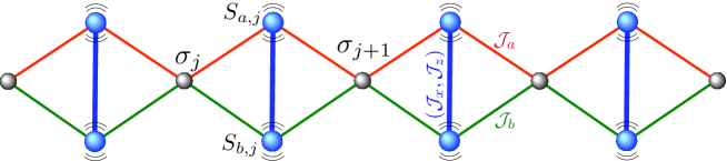
Figure 1: (Colour online) A schematic representation of the spin-1/2 Ising-Heisenberg diamond chain with the magnetoelastic coupling. The Ising spins $\sigma_{j}$ are placed at rigid lattice positions, while the Heisenberg spins $S_{a,j}$ and $S_{b,j}$ harmonically vibrate in a direction perpendicular with respect to the chain axis.

Under this condition, the spin-1/2 Ising-Heisenberg diamond chain can be defined through the Hamiltonian

$${\cal{H}}=\sum_{j=1}^{N}{\cal H}_{j}=\sum_{j=1}^{N}\left({\cal{H}}_{j}^{({\text{p}})}+{\cal{H}}_{j}^{({\text{me}})}\right),$$ (2.1)

where ${\cal H}_{j}^{({\rm p})}$ corresponds to the pure phonon part and ${\cal H}_{j}^{({\rm me})}$ stands for the magnetoelastic part of the Hamiltonian ${\cal H}_{j}$ explicitly given in what follows.

A specification of the displacements within the diamond unit cell is depicted in figure 2 (a), where $x_{0}$ is the equilibrium distance between the Ising spins, $y_{0}$ corresponds to the equilibrium distance between the Heisenberg spins, and $d_{0}$ is the equilibrium distance between the Ising and Heisenberg spins. It is supposed that the decorating atoms $a$ and $b$ including the Heisenberg spins perform harmonic oscillations around their equilibrium lattice positions, which can be characterized through small displacements $y_{a}$ and $y_{b}$, while nodal Ising spins are considered at a rigid position (heavy atoms), this assumption is also reasonable because there is no direct interaction between Ising spins. Consequently, the instantaneous distances between the Heisenberg and Ising spins are changed to $d_{a}=d_{0}+y_{a}\sin({\theta}/{2})$ and $d_{b}=d_{0}+y_{b}\sin({\theta}/{2})$ though the distance $x_{0}$ between the Ising spins remains unaltered. Note that $y_{a}$ and $y_{b}$ are considered positive when dimer particles expand, but when they compress, we consider them negative.

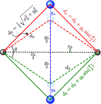
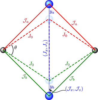
(a)

(b)

Figure 2: (Colour online) A specification of the diamond unit cell under the geometric deformation through the displacements (a) and the exchange interactions (b).

Under the linear approximation, the magnetoelastic part of the bond Hamiltonian (2.1) can be written in this form

$${\cal H}_{j}^{({\rm me})}= -\mathcal{J}_{x,j}\left(S_{a,j}^{x}S_{b,j}^{x}+S_{a,j}^{y}S_{b,j}^{y}\right)-\mathcal{J}_{z,j}S_{a,j}^{z}S_{b,j}^{z}-\left(\mathcal{J}_{a,j}S_{a,j}^{z}+\mathcal{J}_{b,j}S_{b,j}^{z}\right)\left(\sigma_{j}+\sigma_{j+1}\right)$$

$$-h_{\mathrm{H}}\left(S_{a,j}^{z}+S_{b,j}^{z}\right)-\frac{h_{\mathrm{I}}}{2}\left(\sigma_{j}+\sigma_{j+1}\right),$$ (2.2)

where the exchange interactions [see figure 2 (b)] are given by

$$\mathcal{J}_{x,j}\!\!\! = \!\!\!J_{x}\left[1-\kappa(\mathsf{y}_{a,j}+\mathsf{y}_{b,j})\right],\qquad\mathcal{J}_{z,j}=J_{z}\left[1-\kappa(\mathsf{y}_{a,j}+\mathsf{y}_{b,j})\right],$$

$$\mathcal{J}_{a,j}\!\!\! = \!\!\!J_{0}\left[1-\eta\mathsf{y}_{a,j}\sin\left(\frac{\theta}{2}\right)\right],\qquad\mathcal{J}_{b,j}=J_{0}\left[1-\eta\mathsf{y}_{b,j}\sin\left(\frac{\theta}{2}\right)\right].$$ (2.3)

Here, $J_{x}$ and $J_{z}$ correspond to $xy$- and $z$-component of the Heisenberg exchange interaction when assuming the decorating atoms at equilibrium positions. Similarly, $J_{0}$ corresponds to the Ising exchange interaction between the Heisenberg and Ising spins at equilibrium positions. Finally, $\kappa$ is the linear expansion coefficient for the magnetoelastic coupling within the Heisenberg dimers and $\eta$ is the linear expansion coefficient for the magnetoelastic coupling between the Ising and Heisenberg spins. We do not include a term of second-order contribution, because we assume simply a linear dependence as considered in reference [8] and in references therein.

For simplicity, from now on, we will consider the standard atomic units (au) which means the Planck’s constant is $\hbar=1$, Boltzmann constant becomes $k_{\mathrm{B}}=1$, Bohr magneton constant is $\mu_{\mathrm{B}}=1/2$ and the gyromagnetic ratio is estimated as $\gamma\approx 2$, so we have $\mu_{\mathrm{B}}\gamma=1$. Therefore, exchange interaction parameters, external magnetic field, displacements, Hooke’s constant are all in atomic units.

The purely elastic part of the bond Hamiltonian (2.1) can be defined as follows:

$${\cal H}_{j}^{({\rm p})}= \frac{\mathsf{p}_{a,j}^{2}}{2m}\!+\!\frac{\mathsf{p}_{b,j}^{2}}{2m}\!+\!\frac{\bar{K}}{2}\negmedspace\left(\mathsf{y}_{a,j}^{2}\!+\!\mathsf{y}_{b,j}^{2}\right)\!+\!\frac{\mathsf{k}_{{}_{\mathrm{H}}}}{2}\left(\mathsf{y}_{a,j}\!+\!\mathsf{y}_{b,j}\right)^{2},$$ (2.4)

where $\mathsf{p}_{a,j}$ and $\mathsf{p}_{b,j}$ are momenta of the decorating atoms with the mass $m$, $\mathsf{y}_{a,j}$ and $\mathsf{y}_{b,j}$ denote their displacements from equilibrium positions, $\mathsf{k}_{{}_{\mathrm{H}}}$ is the “spring-stiffness” constant ascribed to the Heisenberg coupling, and $\bar{K}=2\mathsf{k}{}_{{}_{\mathrm{I}}}\sin^{2}({\theta}/{2})$ is the effective “spring-stiffness” constant of the Ising coupling when $\mathsf{k}{}_{{}_{\mathrm{I}}}$ is a true “spring-stiffness” constant ascribed to the Ising coupling.

2.1 Local canonical transformation

The Hamiltonian (2.1) involves magnetoelastic and pure elastic (phonon) contributions, which are coupled together through the linear expansion coefficients $\kappa$ and $\eta$ pertinent to the magnetoelastic couplings. However, both contributions can be decoupled through the local canonical coordinate transformation

$$\bm{q}_{j}=\frac{1}{\sqrt{2}}\left(\mathsf{y}_{a,j}+\mathsf{y}_{b,j}\right)\quad\text{and}\quad\bar{\bm{q}}_{j}=\frac{1}{\sqrt{2}}\left(\mathsf{y}_{a,j}-\mathsf{y}_{b,j}\right),$$ (2.5)

which defines the positions of two fictitious particles. Analogously, the momenta in the canonical coordinates take the form

$$\bm{p}_{j}=\frac{1}{\sqrt{2}}\left(\mathsf{p}_{a,j}+\mathsf{p}_{b,j}\right)\quad\text{and}\quad\bar{\bm{p}}_{j}=\frac{1}{\sqrt{2}}\left(\mathsf{p}_{a,j}-\mathsf{p}_{b,j}\right).$$ (2.6)

Thus, the Hamiltonian (2.4) in the canonical coordinates can be rewritten as follows:

$${\cal H}_{j}^{({\rm p})}= \frac{\bm{p}_{j}^{2}}{2m}+\frac{\bar{\bm{p}}_{j}^{2}}{2m}+\frac{\bar{K}}{2}\left(\bm{q}_{j}^{2}+\bar{\bm{q}}_{j}^{2}\right)+\mathsf{k}_{{}_{\mathrm{H}}}\bm{q}_{j}^{2}\,.$$ (2.7)

2.2 Diagonalization of the magnetoelastic part

Since the commutation relation $[{\cal H}_{i}^{({\rm me})},{\cal H}_{j}^{({\rm me})}]=0$ is satisfied, the magnetoelastic part of the bond Hamiltonian (2.2) can be diagonalized separately for each unit cell and the respective eigenvalues can be expressed as a function of the canonical coordinate for a position $\bm{q}_{j}$ in the following form

$$\varepsilon_{k,j}= \mathfrak{e}_{k,j}^{(0)}+\mathfrak{e}_{k,j}^{(1)}\bm{q}_{j}\,,$$ (2.8)

with the first index being $k=\{1,2,3,4\}$ and the second index specifying the unit cell. The eigenvalues (2.8) were decomposed into two terms, whereas the first terms $\mathfrak{e}_{k,j}^{(0)}$ correspond to a fully rigid diamond chain

$$\mathfrak{e}_{1,j}^{(0)}\!\!\! = \!\!\!-\frac{J_{z}}{4}-h_{\mathrm{H}}-\left(\frac{h_{\mathrm{I}}}{2}+J_{0}\right)\mu_{j}\,,\qquad\mathfrak{e}_{2,j}^{(0)}=-\frac{J_{z}}{4}+h_{\mathrm{H}}-\left(\frac{h_{\mathrm{I}}}{2}-J_{0}\right)\mu_{j}\,,$$

$$\mathfrak{e}_{3,j}^{(0)}\!\!\! = \!\!\!\frac{J_{z}}{4}+\frac{J_{x}}{2}-\frac{h_{\mathrm{I}}}{2}\mu_{j}\,,\qquad\qquad\qquad\mathfrak{e}_{4,j}^{(0)}=\frac{J_{z}}{4}-\frac{J_{x}}{2}-\frac{h_{\mathrm{I}}}{2}\mu_{j}\,,$$ (2.9)

which can be alternatively interpreted as the energy eigenvalues when the decorating atoms are at equilibrium positions $y_{a,j}=y_{b,j}=0$ and for simplicity, we denoted $\mu_{j}=(\sigma_{j}+\sigma_{j+1})$. The second terms $\mathfrak{e}_{k,j}^{(1)}$ determine a vibrational contribution to the overall energy, which is given by

$$\mathfrak{e}_{1,j}^{(1)}\!\!\! = \!\!\!\frac{\sqrt{2}}{4}\left[{\it J_{z}}\kappa+2J_{0}\eta\mu_{j}\sin\left(\frac{\theta}{2}\right)\right],\qquad\mathfrak{e}_{2,j}^{(1)}=\frac{\sqrt{2}}{4}\left[{\it J_{z}}\kappa-2J_{0}\eta\mu_{j}\sin\left(\frac{\theta}{2}\right)\right],$$

$$\mathfrak{e}_{3,j}^{(1)}\!\!\! = \!\!\!-\frac{\sqrt{2}}{4}\kappa(2J_{x}+J_{z}),\qquad\qquad\qquad\mathfrak{e}_{4,j}^{(1)}=\frac{\sqrt{2}}{4}\kappa(2J_{x}-J_{z}).$$ (2.10)

The eigenvectors, which correspond to the energy eigenvalues (2.8), can be expressed using the notation $|_{S_{b}^{z}}^{S_{a}^{z}}\rangle_{j}$ as follows

$$|\varphi_{1}\rangle_{j}=|_{+}^{+}\rangle_{j}\,,\quad|\varphi_{2}\rangle_{j} = |_{-}^{-}\rangle_{j}\,,\quad|\varphi_{3}\rangle_{j}=\sin(\vartheta_{j})|{}_{-}^{+}\rangle_{j}-\cos(\vartheta_{j})|{}_{+}^{-}\rangle_{j}\,,$$

$$|\varphi_{4}\rangle_{j} = \cos(\vartheta_{j})|{}_{-}^{+}\rangle_{j}+\sin(\vartheta_{j})|{}_{+}^{-}\rangle_{j}\,,$$

whereas the relevant mixing angle $\vartheta_{j}$ entering the last two eigenvectors is defined as follows:

$$\tan(2\vartheta_{j})=\frac{J_{x}(1-\kappa\sqrt{2}q_{j})}{\sqrt{2}J_{0}\eta\sin(\frac{\theta}{2})\bar{q}_{j}\mu_{j}}\,.$$

It is worth to mention that the last two eigenvectors depend on the positions $q_{j}$ and $\bar{q}_{j}$ of the decorating atoms.

2.3 Diagonalization of the phonon part

After performing the canonical coordinate transformation and diagonalizing, the magnetoelastic part for each eigenvalue of bond Hamiltonian takes the form

$${\cal H}_{k,j}=\mathfrak{e}_{k,j}^{(0)}+\mathfrak{e}_{k,j}^{(1)}\bm{q}_{j}+\frac{\bm{p}_{j}^{2}}{2m}+\frac{\bar{\bm{p}}_{j}^{2}}{2m}+\frac{\bar{K}}{2}\left(\bm{q}_{j}^{2}+\bar{\bm{q}}_{j}^{2}\right)+\mathsf{k}_{{}_{\mathrm{H}}}\bm{q}_{j}^{2}\,.$$ (2.11)

The above result can be subsequently fully decoupled and diagonalized by completing square through an additional local transformation for relative position of the Heisenberg dimers

$$\bm{q}_{j}=\bm{q}_{j}^{\prime}-\frac{\mathfrak{e}_{k,j}^{(1)}}{K}\,,$$ (2.12)

which is defined through the effective spring-stiffness constants $K=\bar{K}+2\mathsf{k}_{{}_{\mathrm{H}}}$ and $\bar{K}=2\mathsf{k}_{{}_{\mathrm{I}}}\sin^{2}({\theta}/{2})$. Substituting a shift of the canonical coordinate for position (2.12) into equation (2.11), one actually achieves a decoupling of the magnetoelastic and pure phonon parts of the bond Hamiltonian, whereas the effective phonon part becomes

$$\mathcal{H}_{j}^{({\rm p})}= \frac{\bm{p}_{j}^{2}}{2m}+\frac{\bar{\bm{p}}_{j}^{2}}{2m}+\frac{K}{2}(\bm{q}_{j}^{\prime})^{2}+\frac{\bar{K}}{2}\bar{\bm{q}}_{j}^{2}\,,$$ (2.13)

while the effective magnetoelastic part reads

$$\mathcal{H}_{k,j}^{({\rm me})}= \mathfrak{e}_{k,j}^{(0)}-\frac{\bigl{(}\mathfrak{e}_{k,j}^{(1)}\bigr{)}^{2}}{2K}\,.$$ (2.14)

To proceed further, let us introduce the annihilation $\bm{b}_{j}$ and creation $\bm{b}_{j}^{\dagger}$ bosonic operators describing phonon positions, which satisfy the standard bosonic commutation relations $[\bm{b}_{j},\bm{b}_{j^{\prime}}^{\dagger}]=\delta_{j,j^{\prime}}$ and $[\bm{b}_{j},\bm{b}_{j^{\prime}}]=0$. The shifted position $\bm{q}^{\prime}_{j}$ and momentum operator $\bm{p}_{j}$ of the Heisenberg dimer can be consequently rewritten in terms of the newly defined creation $\bm{b}_{j}^{\dagger}$ and annihilation $\bm{b}_{j}$ bosonic operators (in units of $\hbar=1$)

$$\bm{q}^{\prime}_{j}=\frac{1}{\sqrt{2m\omega}}(\bm{b}_{j}^{\dagger}+\bm{b}_{j})\quad\text{and}\quad\bm{p}_{j}=i\sqrt{\frac{m\omega}{2}}(\bm{b}_{j}^{\dagger}-\bm{b}_{j}),$$ (2.15)

where $\omega=\sqrt{K/m}$ is the respective phonon frequency. Similarly, one may also introduce the annihilation $\bar{\bm{b}}_{j}$ and creation $\bar{\bm{b}}_{j}^{\dagger}$ bosonic operators describing the corresponding phonon term, which also satisfy the standard bosonic commutation relations $[\bar{\bm{b}}_{j},\bar{\bm{b}}_{j^{\prime}}^{\dagger}]=\delta_{j,j^{\prime}}$ and $[\bar{\bm{b}}_{j},\bar{\bm{b}}_{j^{\prime}}]=0$. Therefore, the position $\bar{\bm{q}}_{j}$ and momentum $\bar{\bm{p}}_{j}$ can be also defined as

$$\bar{\bm{q}}_{j}=\frac{1}{\sqrt{2m\bar{\omega}}}(\bar{\bm{b}}_{j}^{\dagger}+\bar{\bm{b}}_{j})\quad\text{and}\quad\bar{\bm{p}}_{j}=i\sqrt{\frac{m\bar{\omega}}{2}}(\bar{\bm{b}}_{j}^{\dagger}-\bar{\bm{b}}_{j}),$$ (2.16)

where $\bar{\omega}=\sqrt{\bar{K}/m}$ is the respective phonon frequency. The phonon part of the Hamiltonian (2.13) can be subsequently expressed in terms of the number operators $\bm{n}_{j}$ and $\bar{\bm{n}}_{j}$ for two aforedescribed phonons

$$\mathcal{H}_{j}^{({\rm p})}= \left(\frac{1}{2}\!+\!\bm{b}_{j}^{\dagger}\bm{b}_{j}\right)\omega\!+\!\left(\frac{1}{2}\!+\!\bar{\bm{b}}_{j}^{\dagger}\bar{\bm{b}}_{j}\right)\bar{\omega}=\left(\frac{1}{2}\!+\!\bm{n}_{j}\right)\omega\!+\!\left(\frac{1}{2}\!+\!\bar{\bm{n}}_{j}\right)\bar{\omega}.$$ (2.17)

In this way, we have achieved diagonalization of the phonon part of the Hamiltonian (2.17) as the number operators $\bm{n}_{j}$ and $\bar{\bm{n}}_{j}$ acquire the following set of eigenvalues $n_{j}$ and $\bar{n}_{j}\in\{0,1,2,...\}$ with regard to the bosonic character of the underlying operators. It is worthwhile to remark that the bond Hamiltonian $\mathcal{H}_{k,j}=\mathcal{H}_{k,j}^{(\mathrm{me})}+\mathcal{H}_{j}^{(\mathrm{p})}$ is now expressed in a fully diagonal form with regard to the diagonal character of the magnetoelastic (2.14) and the phonon (2.17) parts, which additionally mutually commute with each other, which will be of principal importance for calculation of the partition function presented in section 4.

3 Ground-state phase diagram

Before exploring the magnetoelastic properties, let us first analyze a ground-state phase diagram of the spin-1/2 Ising-Heisenberg diamond chain supplemented with the magnetoelastic coupling, which exhibits three different ground states on the assumption that $k_{\mathrm{H}}=k_{\mathrm{I}}$ and $\kappa=\eta$. The first ground state can be classified as the saturated paramagnetic state (SA) given by the eigenvector

$$|\mathrm{SA}\rangle=\prod_{j=1}^{N}|_{+}^{+}\rangle_{j}|\uparrow\rangle_{j}\,,$$ (3.1)

whereas the former (latter) state vector defines a spin state of the Heisenberg dimer (the Ising spin) from the $j$th unit cell. The saturated paramagnetic state has the following eigenenergy

$$E_{\mathrm{SA}}=-\frac{J_{z}}{4}-h_{\mathrm{H}}-\frac{h_{\mathrm{I}}}{2}-J_{0}-\frac{\left({\it J_{z}}\kappa+2J_{0}\eta\sin\frac{\theta}{2}\right)^{2}}{16K}\,.$$ (3.2)

The second ground state can be viewed as the classical ferrimagnetic phase (FI₁) given by the eigenvector

$$|\mathrm{FI}_{1}\rangle=\prod_{j=1}^{N}|_{+}^{+}\rangle_{j}|\downarrow\rangle_{j}\,,$$ (3.3)

whereas the corresponding energy becomes

$$E_{\mathrm{FI}_{1}}=-\frac{J_{z}}{4}-h_{\mathrm{H}}+\frac{h_{\mathrm{I}}}{2}+J_{0}-\frac{\left({\it J_{z}}\kappa-2J_{0}\eta\sin\frac{\theta}{2}\right)^{2}}{16K}\,.$$ (3.4)

The sublattice magnetization of the Ising spins is $M_{\mathrm{I}}=-1/2$ per unit cell, the sublattice magnetization of the Heisenberg spins is $M_{\mathrm{H}}=1$ per unit cell so that the total magnetization per unit cell is $M_{\mathrm{t}}=1/2$. The third ground state can be classified as the quantum ferrimagnetic phase (FI₂) given by the eigenvector

$$|\mathrm{FI}_{2}\rangle=\prod_{j=1}^{N}\left(\cos(\vartheta_{j})|{}_{-}^{+}\rangle_{j}+\sin(\vartheta_{j})|{}_{+}^{-}\rangle_{j}\right)|\uparrow\rangle_{j}\,,$$ (3.5)

whose corresponding eigenenergy reads as follows:

$$E_{\mathrm{FI}_{2}}=\frac{J_{z}}{4}-\frac{J_{x}}{2}-\frac{h_{\mathrm{I}}}{2}-\frac{\kappa^{2}(2J_{x}-J_{z})^{2}}{16K}\,.$$ (3.6)

The sublattice magnetization of the Heisenberg spins is $M_{\mathrm{H}}=0$ due to a singlet-like character of the Heisenberg dimers and hence, the sublattice magnetization of the Ising spins $M_{\mathrm{I}}=1/2$ provides the only nonzero contribution to the total magnetization per unit cell $M_{\mathrm{t}}=1/2$.

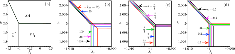
Figure 3: (Colour online) Ground-state phase diagram in $J_{z}-h$ plane for $J_{0}=-1$, $J_{x}=1$ and: (a)–(b) $\kappa=0.5$, $\theta=\piup/2$ and $k_{\mathrm{H}}=\{25,50,200,1000\}$; (c) $\kappa=0.5$, $k_{\mathrm{H}}=50$ and $\theta=\{2\piup/3,\piup/2,\piup/3,\piup/4,\piup/8\}$; (d) $\theta=\piup/3$, $k_{\mathrm{H}}=50$ and $\kappa=\{0.1,0.2,0.3,0.4,0.5\}$.

Here, we consider the local magnetic fields $h=h_{\mathrm{I}}=h_{\mathrm{H}}$ acting on the Ising and Heisenberg spins, which physically corresponds to the equality of their Landé g-factors. A few typical ground-state phase diagrams are plotted in figure 3 in $J_{z}-h$ plane for the fixed values of the coupling constants $J_{0}=-1$ and $J_{x}=1$. It is evident that the ground-state phase boundaries are only gradually shifted with respect to a perfectly rigid limit when assuming realistic (rather high) values of the spring-stiffness constants (see [36] for a comparison). As a matter of fact, the changes in the ground-state phase diagram shown in figure 3 (a) for the fixed values of $\kappa=0.5$ and $\theta=\piup/2$ due to variation of the spring-stiffness constant $k_{\mathrm{H}}=\{25,50,200,1000\}$ are almost indistinguishable within the displayed scale, while they become evident just in a magnified scale as illustrated in figure 3 (b). Note that similar effects also result from the changes of other interaction parameters [see figure 3 (c)–(d)]. The role of lattice geometry can be traced back in figure 3 (c), where the ground-state phase diagrams are plotted for fixed values of $\kappa=0.5$, $k_{\mathrm{H}}=50$ and several values of the angle $\theta=\{2\piup/3,\piup/2,\piup/3,\piup/4,\piup/8\}$. Finally, the effect of magnetoelastic constant on the ground-state phase diagrams is illustrated in figure 3 (d) when assuming a fixed value of $\theta=\piup/3$, $k_{\mathrm{H}}=50$ upon variation of $\kappa=\{0.1,0.2,0.3,0.4,0.5\}$.

The phase boundary between two ferrimagnetic phases FI₁ and FI₂ is given by

$$J_{z}=\frac{\left[4\!\left(2J_{0}\!+\!J_{x}\right)\!k_{\mathrm{H}}\!-\!J_{0}^{2}\kappa^{2}\right]\!\left(\sin^{2}\frac{\theta}{2}+1\right)\!+\!\left(J_{0}^{2}\!+\!J_{x}^{2}\right)\!\kappa^{2}}{\kappa^{2}\left(J_{x}-J_{0}\sin\frac{\theta}{2}\right)+4k_{\mathrm{H}}\left(\sin^{2}\frac{\theta}{2}+1\right)}\,,$$ (3.7)

which is independent of the magnetic field $h$ as evidenced by a vertical character of the relevant phase boundaries in figure 3. The phase boundary between the phases FI₁ and SA follows from the formula

$$h=-2J_{0}-\frac{J_{0}J_{z}\kappa^{2}\sin\frac{\theta}{2}}{4{\it k}_{\mathrm{H}}\left(\sin^{2}\frac{\theta}{2}+1\right)}\,.$$ (3.8)

While this phase boundary is for a perfectly rigid model ($\kappa=0$) completely independent of $J_{z}$, the model with nonzero magnetoelastic coupling constant $\kappa\neq 0$ shows a relatively weak dependence on the coupling constant $J_{z}$ because $\kappa$ is in general a very small quantity ($\kappa\ll 1$), while the spring-stiffness constant $k_{\mathrm{H}}\gg\mathfrak{e}_{k,j}^{(1)}$ [i.e. $k_{\mathrm{H}}\gg J_{0}J_{z}$, see figure 3 (b)–(d) for illustration]. A similar finding concerns with the phase boundary between FI₂ and SA phases, which is given by

$$h= \frac{1}{2}\left(J_{x}-2J_{0}-J_{z}\right)+\kappa^{2}\frac{\left({\it J_{x}}+J_{0}\sin\frac{\theta}{2}\right)\left({\it J_{x}}-J_{z}-J_{0}\sin\frac{\theta}{2}\right)}{8k_{\mathrm{H}}\left(\sin^{2}\frac{\theta}{2}+1\right)}\,.$$ (3.9)

This phase boundary depends on the coupling constant $J_{z}$ even in the perfectly rigid limit ($\kappa=0$), but there appears a small correction to this dependence once nonzero magnetoelastic coupling constant ($\kappa\neq 0$) is taken into consideration.

4 Thermodynamics

As previously commented, the phonon $\mathcal{H}_{j}^{(\mathrm{p})}$ and magnetoelastic $\mathcal{H}_{k,j}^{(\mathrm{me})}$ parts of the bond Hamiltonian [2.14 and (2.17)] commute with each other. For this reason, the bond Hamiltonians corresponding to two different unit cells also satisfy the commutation relation $[{\cal H}_{j},{\cal H}_{j^{\prime}}]=0$. The partition function of the spin-1/2 Ising-Heisenberg diamond chain accounting for the magnetoelastic interaction can be accordingly obtained by using the transfer-matrix approach. A decoupled character of the phonon and magnetoelastic parts of the Hamiltonian allows one to factorize the partition function into a product of two terms

$$\mathcal{Z}_{N}={\cal Z}_{N}^{(\mathrm{p})}{\cal Z}_{N}^{(\mathrm{me})},$$ (4.1)

whereas the former one ${\cal Z}_{N}^{(\mathrm{p})}$ denotes the phonon contribution and the latter one ${\cal Z}_{N}^{(\mathrm{me})}$ corresponds to the magnetoelastic contribution. It is noteworthy that the phonons corresponding to $(\bm{p},\bm{q})$ and $(\bar{\bm{p}},\bar{\bm{q}})$ of the Heisenberg dimers are independent of each other and hence, the phonon part of the partition function can be expressed more explicitly as follows

$${\cal Z}_{N}^{(\mathrm{p})}=\left(u\bar{u}\right)^{N},$$ (4.2)

where individual contributions stemming from two kinds of phonons involved in the Hamiltonian (2.14) follow from a summation over all accessible values of the quantum numbers $n_{j}$ and $\bar{n}_{j}$

$$u=\sum_{n_{j}=0}^{\infty}{\rm e}^{-\beta\left(\frac{1}{2}+n_{j}\right)\omega}=\frac{1}{2{\rm sinh}\left(\frac{\beta\omega}{2}\right)},\qquad\bar{u}=\sum_{\bar{n}_{j}=0}^{\infty}{\rm e}^{-\beta\left(\frac{1}{2}+\bar{n}_{j}\right)\bar{\omega}}=\frac{1}{2{\rm sinh}\left(\frac{\beta\bar{\omega}}{2}\right)}\,.$$ (4.3)

The magnetoelastic part of the partition function can be calculated using the transfer matrix

$$\bm{W}=\left(\begin{array}[]{cc}w_{1}&w_{0}\\ w_{0}&w_{-1}\end{array}\right),$$ (4.4)

which involves the Boltzmann factors of the $j$th Heisenberg dimer defined as follows:

$$w_{\mu_{j}}=\sum_{k=1}^{4}{\rm e}^{-\beta\bigl{[}\mathfrak{e}_{k,j}^{(0)}-\frac{1}{2K}\bigl{(}\mathfrak{e}_{k,j}^{(1)}\bigr{)}^{2}\bigr{]}}\,.$$ (4.5)

In the above, the energy contributions $\mathfrak{e}_{k,j}^{(0)}$ and $\mathfrak{e}_{k,j}^{(1)}$ are given by equations (2.9) and (2.10), respectively. After a straightforward diagonalization of the transfer matrix (4.4), one gets two eigenvalues

$$\lambda_{\pm}=\frac{1}{2}\left(w_{1}+w_{-1}\pm\sqrt{(w_{1}-w_{-1})^{2}+4w_{0}^{2}}\right).$$ (4.6)

The magnetoelastic part of the partition function can be expressed via the transfer-matrix eigenvalues

$${\cal Z}_{N}^{(\mathrm{me})}=\lambda_{+}^{N}+\lambda_{-}^{N}\,.$$ (4.7)

At this stage, one may substitute the phonon and magnetoelastic parts of the partition functions (4.2 and (4.7)) into equation (4.1) in order to get the final result for the partition function and the associated free energy, which in the thermodynamic limit reduces to the form

$$f=-\frac{1}{\beta}\lim_{N\to\infty}\frac{1}{N}\ln{\cal Z}_{N}=-\frac{1}{\beta}\ln\left(u\bar{u}\right)-\frac{1}{\beta}\ln\left(\lambda_{+}\right).$$ (4.8)

With the free energy in hand, we are able to discuss magnetoelastic properties of the spin-1/2 Ising-Heisenberg diamond chain at nonzero temperatures.

In what follows our particular attention will be devoted to the magnetoelastic behavior at and near a triple point, where all three phases SA, FI₁ and FI₂ coexist together at zero temperature. In the case of a completely rigid model ($\kappa=\eta=0$), the three phases coexist together for fixed parameters $J_{0}=-1$, $J_{x}=1$, $J_{z}=-1$ when the magnetic field $h\rightarrow 2$ [see in figure 3 (a)]. After some algebraic manipulations, one obtains the following asymptotic expression for the free energy of the rigid model $f_{0}=-T\ln\left(\lambda_{+}\right)$ in the zero-temperature limit $T\rightarrow 0$

$$f_{0}= E_{0}-T\ln\left(\frac{3+\sqrt{5}}{2}\right)-\frac{\sqrt{5}}{10}\left(h_{\mathrm{I}}-2\right)-\frac{1}{2}\left(1+\frac{\sqrt{5}}{5}\right)\left(h_{\mathrm{H}}-2\right),$$ (4.9)

where $E_{0}=E_{\mathrm{FI}_{2}}=E_{\mathrm{FI}_{1}}=E_{\mathrm{SA}}$ defines the corresponding ground-state energy at a triple point. Now, one may differentiate the free energy (4.9) in order to calculate the entropy

$$\mathcal{S}_{0}=-\left(\frac{\partial f_{0}}{\partial T}\right)_{h}=\ln\left(\frac{3+\sqrt{5}}{2}\right)\approx 0.962423,$$ (4.10)

the sublattice magnetization of the Ising spins $M_{\mathrm{I},0}=-\left({\partial f_{0}}/{\partial h_{\mathrm{I}}}\right)_{T}={\sqrt{5}}/{10}$, the sublattice magnetization of the Heisenberg spins $M_{\mathrm{H},0}=-\left({\partial f_{0}}/{\partial h_{\mathrm{H}}}\right)_{T}=1/2\cdot\left(1+{\sqrt{5}}/{5}\right),$ while the total magnetization per unit cell equals

$$M_{\mathrm{t},0}=M_{\mathrm{I},0}+M_{\mathrm{H},0}=\frac{1}{2}+\frac{\sqrt{5}}{5}\approx 0.9472136.$$ (4.11)

This exact result will be confirmed later by numerical computation at finite temperatures.

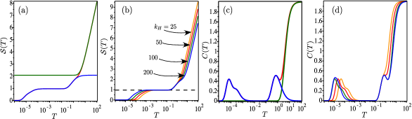
Figure 4: (Colour online)  (a) The entropy as a function of temperature in a semi-logarithmic scale for fixed values of $k_{\mathrm{H}}=100$, $\kappa=0.5$, $J_{0}=-1$, $J_{x}=1$, $J_{z}=-1$, $\theta=\piup/2$ and $h=2$. A blue line corresponds to the rigid model, a green line describes the phonon contribution and a red line reports the overall entropy of the model with the magnetoelastic coupling; (b) The overall entropy as a function of temperature in a semi-logarithmic scale for fixed values of $\kappa=0.5$, $J_{0}=-1$, $J_{x}=1$, $J_{z}=-1$, $\theta=\piup/2$, $h=2$ and four different values of $k_{\mathrm{H}}=\{25,50,100,200\}$; (c) Temperature variations of the specific heat corresponding to the panel (a); (d) Temperature variations of the specific heat corresponding to the panel (b).

Now, let us compare the magnetic behavior of the model accounting for the magnetoelastic coupling in the vicinity of the triple point with that of the fully rigid model in order to find out differences arising from the magnetoelastic coupling. To this end, the entropy is plotted in figure 4 (a) as a function of temperature in semi-logarithmic scale, whereas a blue line corresponds to the fully rigid model, a green line describes the phonon contribution and a red line reports the overall entropy for the fixed values $k_{\mathrm{H}}=100$, $\kappa=0.5$, $J_{0}=-1$, $J_{x}=1$, $J_{z}=-1$, $\theta=\piup/2$ and $h=2$. It can be seen that the entropy closely follows the entropy of the rigid model at low enough temperatures, whereas it tends to the phonon contribution at a sufficiently high temperature. Figure 4 (c) depicts the temperature dependencies of the specific heat corresponding to figure 4 (a). Figure 4 (b) illustrates the overall entropy of the model accounting for the magnetoelastic coupling for the fixed values of $\kappa=0.5$, $J_{0}=-1$, $J_{x}=1$, $J_{z}=-1$, $\theta=\piup/2$, $h=2$ and four different values of the spring-stiffness constant $k_{\mathrm{H}}=\{25,50,100,200\}$. It is evident from this figure that the entropy displays a plateau at $\mathcal{S}_{0}=\ln[{(3+\sqrt{5})}/{2}]$ regardless of the spring-stiffness constant in the range of moderate temperatures $10^{-3}\lesssim T\lesssim 10^{-1}$ before it tends to zero in the asymptotic limit $T\to 0$. Note that the fully rigid model $(k_{\mathrm{H}}\rightarrow\infty)$ exhibits, for the considered set of parameters, the residual entropy $\mathcal{S}_{0}=\ln[{(3+\sqrt{5})}/{2}]$, which is however lifted for finite values of the spring-stiffness constant due to the shift of the ground-state phase boundaries. Finally, figure 4 (d) depicts temperature variations of the specific heat corresponding to figure 4 (b), where the formation of the additional small peak can be observed in a low-temperature region due to the respective changes of the entropy from a nonzero plateau to null.

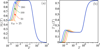
Figure 5: (Colour online) (a) The total magnetization per unit cell as a function of temperature in a semi-logarithmic scale for fixed values of $\kappa=0.5$, $J_{0}=-1$, $J_{x}=1$, $J_{z}=-1$, $\theta=\piup/2$, $h=2$ and four different values of $k_{\mathrm{H}}=\{25,50,100,200\}$; (b) A semi-logarithmic plot of the magnetic susceptibility times temperature ($\chi T$) product for the same parameter set as used in figure 5 (a) for the magnetization.

The total magnetization is depicted in figure 5 (a) against the temperature in a semi-logarithmic scale by assuming fixed values of $\kappa=0.5$, $J_{0}=-1$, $J_{x}=1$, $J_{z}=-1$, $\theta=\piup/2$, $h=2$ and four different values of the spring-stiffness constant $k_{\mathrm{H}}=\{25,50,100,200\}$. It turns out that the total magnetization per unit cell tends in the zero-temperature limit to the initial value $M_{\mathrm{t}}=0.5$ irrespective of the spring-stiffness constant. Then it increases in agreement with the formula (4.11) to the value $M_{\mathrm{t}}\sim 0.947$ in the range of moderate temperatures $10^{-3}\lesssim T\lesssim 10^{-1}$ before it finally tends to zero in the high-temperature region. Figure 5 (b) illustrates the respective temperature variations of the magnetic susceptibility times temperature ($\chi T$) product for the same set of parameters as used in figure 5 (a) for the magnetization. It is obvious that the product vanishes $\chi T\rightarrow 0$ as temperature tends to zero, an intermediate plateau around the value $\chi T\sim 0.18$ is found at moderate temperatures $10^{-3}\lesssim T\lesssim 10^{-1}$ and the product reaches the asymptotic value $\chi T\sim 0.8$ in the high-temperature limit.

5 Conclusions

In the present paper we have examined in detail the magnetoelastic properties of the spin-1/2 Ising-Heisenberg diamond chain, which involves two Heisenberg spins and one nodal Ising spin in each unit cell. It is supposed that the decorating atoms involving the Heisenberg spins harmonically vibrate perpendicular to the chain axis, while the nodal atoms involving the Ising spins are placed at rigid lattice positions when completely neglecting their lattice vibrations. In particular, we have first investigated the ground-state phase diagram depending on the magnetoelastic constant and the spring-stiffness constant ascribed to the Heisenberg coupling with the main emphasis laid on an investigation of the parameter region close to a triple coexistence point of two ferrimagnetic phases and one saturated paramagnetic phase. Next, we have also examined in detail the thermodynamic properties at nonzero temperatures.

It has been found that the magnetoelastic nature of the Heisenberg dimers is reflected through a nonzero plateau of the entropy in a low-temperature region, whereas the specific heat displays an anomalous peak slightly below the temperature region corresponding to the entropy plateau. It also turns out that the magnetization exhibits a plateau at almost saturated value in the same temperature region as the entropy before it gradually tends to zero upon further increase of temperature. The magnetic susceptibility displays within the plateau region an inverse temperature dependence, which slightly drops above this plateau, whereas an inverse temperature dependence is repeatedly recovered at high enough temperatures.

Ukrainian 0

Ìàãíåòîåëàñòèчíi âëàñòèâîñòi ñïií-1/2 ðîìáiчíîãî ëàíöþæêà Içiíґà-Ãàéçåíáåðґà ïîáëèçó ïîòðiéíî¿ òîчêè ñïiâiñíóâàííÿ

Í. Ôåððåéðà${}^{\textsf{\footnotesize{\mbox{?}}}}$, Äæ. Òîððiêî${}^{\textsf{\footnotesize{\mbox{?}}}}$, Ñ.Ì. äå Ñîóçà${}^{\textsf{\footnotesize{\mbox{?}}}}$, Î. Ðîõàñ${}^{\textsf{\footnotesize{\mbox{?}}}}$, É. Ñòðåчêà${}^{\textsf{\footnotesize{\mbox{?}}}}$

             
${}^{\textsf{\footnotesize 1}}$ Êàôåäðà ôiçèêè, Ôåäåðàëüíèé óíiâåðñèòåò Ëàâðàñà, C. P. 3037, 37200-900, Ëiâðàñ, Ìiíà Æåðå,
Áðàçèëiÿ ${}^{\textsf{\footnotesize 2}}$ Êàôåäðà ôiçèêè, Ôåäåðàëüíèé óíiâåðñèòåò Ìiíà Æåðå, C. P. 702, 30123-970, Áåëó-Îðèçîíòi,
Ìiíà Æåðå, Áðàçèëiÿ ${}^{\textsf{\footnotesize 3}}$ Iíñòèòóò ôiçèêè, Ôàêóëüòåò ïðèðîäíèчèõ íàóê, Óíiâåðñèòåò iìåíi Ï. É. Øàôàðèêà, ïàðê Àíãåëiíóì 9, Êîøèöi 04001, Ñëîâàччèíà

References

- [1] Henriques V.B., Salinas S.R., J. Phys. C: Solid State Phys., 1987, 20, 2415, doi:10.1088/0022-3719/20/16/014.
- [2] Massimino P., Diep H.T., J. Appl. Phys., 2000, 87, 7043, doi:10.1063/1.372925.
-
[3]
Boubcheur E., Massimino P., Diep H.T., J. Magn.
Magn. Mater., 2001, 223, 163,
doi:10.1016/S0304-8853(00)00752-6. - [4] Armstrong W.D., Mater. Sci. Eng., B, 1997, 47, 47, doi:10.1016/S0921-5107(97)02040-0.
-
[5]
Tickle R., James R.D., Shield T., Wuttig M.,
Kokorin V.V., IEEE Trans. Magn., 1999, 35, 4301,
doi:10.1109/20.799080. - [6] Tickle R., James R.D., J. Magn. Magn. Mater., 1999, 195, 627, doi:10.1016/S0304-8853(99)00292-9.
- [7] Strečka J., Rojas O., de Souza S.M., Phys. Lett. A, 2012, 376, 197, doi:10.1016/j.physleta.2011.11.008.
-
[8]
Strečka J., Rebič M., Rojas O., de Souza S.M., J. Magn. Magn. Mater., 2019, 469, 655,
doi:10.1016/j.physleta.2019.05.017. - [9] Enting I.G., J. Phys. A: Math. Nucl. Gen., 1973, 6, 170, doi:10.1088/0305-4470/6/2/008.
-
[10]
Jaščur M., Štubňa V., Szalowski K.,
Balcerzak T., J. Magn. Magn. Mater., 2016, 417,
92, doi:10.1016/j.jmmm.2016.05.048. - [11] Štubňa V., Jaščur M., J. Magn. Magn. Mater., 2017, 442, 364, doi:10.1016/j.jmmm.2017.07.011.
- [12] Fisher M.E., Phys. Rev., 1959, 113, 969, doi:10.1103/PhysRev.113.969.
-
[13]
Syozi I., In: Phase Transitions and Critical Phenomena, Vol. 1,
C. Domb and M. S. Green (Eds.),
Academic Press, New York, 1972. - [14] Rojas O., Valverde J.S., de Souza S.M., Physica A, 2009, 388, 1419, doi:10.1016/j.physa.2008.12.063.
- [15] Strečka J., Phys. Lett. A, 2010, 374, 3718, doi:10.1016/j.physleta.2010.07.030.
- [16] Rojas O., de Souza S.M., J. Phys. A: Math. Theor., 2011, 44, 245001, doi:10.1088/1751-8113/44/24/245001.
- [17] Mattis D.C., Schultz T.D., Phys. Rev., 1963, 129, 175, doi:10.1103/PhysRev.129.175.
- [18] Salinas S.R., J. Phys. A: Math. Nucl. Gen., 1973, 6, 1527, doi:10.1088/0305-4470/6/10/011.
- [19] Kneževič M., Miloševič S., J. Phys. A: Math. Gen., 1980, 13, 2479, doi:10.1088/0305-4470/13/7/029.
-
[20]
Lemos C.G.O., Santos M., Ferreira A.L.,
Figuereido W., Phys. Rev. E, 2019, 99, 012129,
doi:10.1103/PhysRevE.99.012129. -
[21]
Balcerzak T., Szałowski K., Jaščur M.,
J. Magn. Magn. Mater., 2020, 507, 166825,
doi:10.1016/j.jmmm.2020.166825. - [22] Qi Y., Jia L., Yu N., Du A., Solid State Commun., 2016, 233, 1, doi:10.1016/j.ssc.2016.02.001.
- [23] Derzhko O., Strečka J., Gálisová L., Eur. Phys. J. B, 2013, 86, 88, doi:10.1140/epjb/e2013-30979-4.
- [24] Lisnyi B., Strečka J., Phys. Status Solidi B, 2014, 251, 1083, doi:10.1002/pssb.201350393.
- [25] Lisnyi B., Strečka J., Physica A, 2016, 462, 104, doi:10.1016/j.physa.2016.06.088.
- [26] Ananikian N., Strečka J., Hovhannisyan V., Solid State Commun., 2014, 194, 48, doi:10.1016/j.ssc.2014.06.015.
- [27] Ananikian N.S., Hovhannisyan V.V., Physica A, 2013, 392, 2375, doi:10.1016/j.physa.2013.01.040.
- [28] Torrico J., Ohanyan V., Rojas O., J. Magn. Magn. Mater., 2018, 454, 85, doi:10.1016/j.jmmm.2018.01.044.
- [29] Gálisová L., Condens. Matter Phys., 2014, 17, 13001, doi:10.5488/CMP.17.13001.
- [30] De Souza S.M., Rojas O., Solid State Commun., 2018, 269, 131, doi:10.1016/j.ssc.2017.10.006.
- [31] Gálisová L., Strečka J., Phys. Rev. E, 2015, 91, 022134, doi:10.1103/PhysRevE.91.022134.
-
[32]
Torrico J., Rojas M., de Souza S.M., Rojas O., Phys.
Lett. A, 2016, 380, 3655,
doi:10.1016/j.physleta.2016.08.007. -
[33]
Carvalho I.M., Torrico J., de Souza S.M., Rojas O.,
Derzhko O., Ann. Phys., 2019,
402, 45, doi:10.1016/j.aop.2019.01.001. -
[34]
Rojas O., Strečka J., Lyra M.L., de Souza S.M., Phys. Rev. E, 2019,
99, 042117, doi:10.1103/PhysRevE.99.042117. - [35] Derzhko O., Krupnitska O., Lisnyi B., Strečka J., EPL, 2015, 112, 37002, doi:10.1209/0295-5075/112/37002.
- [36] Čanová L., Strečka J., Jaščur M., J. Phys.: Condens. Matter, 2006, 18, 4967, doi:10.1088/0953-8984/18/20/020.
Ukrainian \adddialect\l@ukrainian0 \l@ukrainian