Microscopic theory of high-temperature superconductivity in
strongly correlated electronic systems ††thanks: The paper is devoted to the 60-th
birthday of Professor A. Shvaika
Abstract
A consistent microscopic theory of superconductivity for strongly correlated electronic systems is presented. The Dyson equation for the normal and anomalous Green functions for the projected (Hubbard) electronic operators is derived. To compare various mechanisms of pairing, the extended Hubbard model is considered where the intersite Coulomb repulsion and the electron-phonon interaction are taken into account. We obtain the -wave pairing with high- induced by the strong kinematical interaction of electrons with spin fluctuations, while the Coulomb repulsion and the electron-phonon interaction are suppressed for the -wave pairing. These results support the spin-fluctuation mechanism of high-temperature superconductivity in cuprates previously proposed in phenomenological models.
Key words: strongly correlated electron systems, Hubbard model, unconventional superconductivity, cuprate superconductors
Abstract
Ïðåäñòàâëåíî ïîñëiäîâíó ìiêðîñêîïiчíó òåîðiþ íàäïðîâiäíîñòi äëÿ ñèëüíîñêîðåëüîâàíèõ åëåêòðîííèõ ñèñòåì. Âèâåäåíî ðiâíÿííÿ Äàéñîíà äëÿ íîðìàëüíî¿ òà àíîìàëüíî¿ ôóíêöié Ґðiíà íà ìîâi ïðîåêöiéíèõ (ãàáàðäiâñüêèõ) åëåêòðîííèõ îïåðàòîðiâ. Äëÿ ïîðiâíÿííÿ ðiçíèõ ìåõàíiçìiâ ñïàðþâàííÿ, áóëî ðîçãëÿíóòî óçàãàëüíåíó ìîäåëü Ãàáàðäà, äå âðàõîâàíî ìiæâóçëîâå êóëîíiâñüêå âiäøòîâõóâàííÿ i åëåêòðîí-ôîíîííó âçàєìîäiþ. Ìè îòðèìàëè -õâèëüîâå ñïàðþâàííÿ ç âèñîêîþ , ùî çóìîâëåíî ñèëüíîþ êiíåòèчíîþ âçàєìîäiєþ åëåêòðîíiâ çi ñïiíîâèìè ôëóêòóàöiÿìè, òîäi ÿê êóëîíiâñüêå âiäøòîâõóâàííÿ òà åëåêòðîí-ôîíîííà âçàєìîäiÿ ïðè -õâèëüîâîìó ñïàðþâàííi ïîñëàáëþþòüñÿ. Öi ðåçóëüòàòè óçãîäæóþòüñÿ ç ñïií-ôëóêòóàöiéíèì ìåõàíiçìîì âèñîêîòåìïåðàòóðíî¿ íàäïðîâiäíîñòi â êóïðàòàõ, ùî ðàíiøå áóâ çàïðîïîíîâàíèé ó ôåíîìåíîëîãiчíèõ ìîäåëÿõ.
Ключовi слова: ñèëüíîñêîðåëüîâàíi åëåêòðîííi ñèñòåìè, Ãàáàðäîâà ìîäåëü, íåçâèчàéíà íàäïðîâiäíiñòü, êóïðàòíi íàäïðîâiäíèêè
1 Introduction
Intensive experimental investigations of high-temperature superconductivity (HTSC) in copper-oxides (cuprates) discovered by Bednorz and Müller [1] more than 30 years ago produced a detailed information concerning unconventional physical properties of cuprates (see, e.g., reference [2]). However, the corresponding theoretical studies of various microscopical models have not yet resulted in a commonly accepted theory of HTSC. The main problem in the theoretical study is that the conventional Fermi-liquid approach fails to describe the electronic structure of the cuprates due to strong electron correlations [3]. They are Mott-Hubbard (more accurately, charge-transfer) antiferromagnetic (AF) insulators where the conduction band splits into two Hubbard subbands: the filled singly occupied subband and the empty doubly occupied ones. They become poor conductors when doped by holes or electrons in the corresponding subbands. To describe such strongly correlated metal one has to use for the subbands the projected (Hubbard) electronic operators which are difficult to treat. Various theoretical methods were used to take into account the complicated non-Fermionic character of these operators, such as numerical simulation for finite clusters, variational approach, diagram technique, cluster approximations, slave boson (electron) representation, etc. (see references [2, 4]).
Recently, we have developed a microscopic theory of spin excitations [5, 6] and superconductivity [7, 8, 9, 10, 11] for cuprates. We employed the equation of motion method for the thermodynamic Green functions [12, 13] (GFs) in terms of the Hubbard operators (HOs) which enabled us to take into account rigorously the non-Fermionic character of electronic operators. We emphasize that the commutation relations for HOs result in the specific kinematical interaction which plays an important role in studying strongly correlated electronic systems. In this paper we present the results of these investigations.
In the next section 2 we consider the Hubbard model of an electronic system with strong correlations and explain how the kinematical interaction appears in the model. Then, we describe the theory of superconductivity developed in our studies. To disclose the mechanism of HTSC, we consider in section 3 the extended Hubbard model where we can compare contributions from the spin-fluctuations and the electron-phonon interaction (EPI) and evaluate a role of the intersite Coulomb interaction (CI). The exact Dyson equation for the normal and anomalous (pair) GFs is derived for this model which is solved in the self-consistent Born approximation (SCBA) for the self-energy. In section 4 the equation for the superconducting order parameter is considered. We found the -wave pairing with high- mediated by the kinematical electron interaction with spin-excitations. can be suppressed only for a large intersite CI of the order of kinematical interaction, much larger than EPI. This supports the spin-fluctuation mechanism of high- in cuprates. In conclusion we summarize our results.
2 Kinematical interaction
The problem of the many-body effects caused by strong electron correlations in solids is one of the most difficult ones which has not yet found a comprehensive solution. Strong electron correlations are usually treated within specific models in which only few relevant electronic states are taken into account (for a review see [3, 4]). In the simplest approximation, one can consider a one-band model and take into account only a single-electron hopping matrix element between the nearest neighbors and a large single-site Coulomb energy . In this approximation, the complicated multiband electronic model of cuprates is reduced to the so-called Hubbard model [14]:
| (2.1) |
where () are the creation (annihilation) operators for electrons of spin at the lattice site and is the electron occupation number. In the limit of strong correlation, , the conduction band splits into two subbands for the singly occupied and doubly occupied states. In this case, to describe the electronic excitations, one has to use the projected electron operators referring to these subbands: where . It is convenient to use the HO representation [15]:
| (2.2) |
The matrix of HOs describes the transition from the state to the state on a lattice site taking into account four possible electronic states: an empty state , a singly occupied electronic state , and a doubly occupied electronic state . The number operator and the spin operators in terms of the HOs are defined as
| (2.3) | |||||
| (2.4) |
From the multiplication rule for the HOs, , there follow their commutation relations
| (2.5) |
with the upper sign for the Fermi-type operators (such as ) and the lower sign for the Bose-type operators (such as the number or spin operators). The HOs obey the completeness relation
| (2.6) |
which rigorously preserves the local constraint that only one quantum state can be occupied on any lattice site . This no-double-occupancy restriction is the most difficult property of the projected electronic operators which is considered in many theoretical approaches in mean-field approximation (MFA) resulting in unjustified results.
The unconventional commutation relations (2.5) for HOs result in the kinematical interaction. The term was introduced by Dyson in a general theory of spin-wave interactions [16] for the spin-wave creation and annihilation operators for spin-. It appears that they are Bose operators on different lattice sites and Fermi operators on the same lattice site. Similar commutation relations hold for the electron creation and annihilation operators,
| (2.7) |
Therefore, the HOs for electrons can be considered as Fermi operators on different lattice sites but on the same lattice site electron kinematical interaction occurs with charge and spin fluctuations. This results in dressing the electron hopping by spin and charge fluctuations with the coupling constant of the order of the kinetic energy (for a two dimensional lattice). The latter is much larger than the antiferromagnetic exchange interaction proposed by Anderson [17] as the coupling parameter for superconducting pairing in cuprates. The superconducting pairing induced by the kinematical interaction for the HOs was first proposed by Zaitsev and Ivanov [18, 19, 20]. However, they found in the MFA the momentum-independent -wave superconducting gap which violates the no-double-occupancy restriction as was shown in references [21, 22]. The spin-fluctuation pairing in the second order of the kinematical interaction beyond the MFA should be taken into account which results in the -wave pairing as discussed below.
3 Green function equations
We apply our theory for consideration of HTSC in cuprate superconductors. To compare electron-phonon and spin-fluctuation pairing mechanisms, we consider the extended Hubbard model which includes the intersite CI and the EPI . In terms of the HOs, the model reads:
| (3.1) | |||||
| (3.2) |
where is the single-electron hopping parameter between lattice sites and , is the single-particle energy and is the two-particle energy, is the chemical potential. describes an atomic displacement on the lattice site for a particular phonon mode. We emphasize that in the Hubbard model (3.1) there is no dynamical coupling of electrons (holes) with spin or charge fluctuations. Its role is played by the kinematical interaction as was discussed in the previous section.
To consider the superconducting pairing in the model (3.1), we introduce the thermodynamic GF [13] using the four-component Nambu operators, and :
| (3.3) |
where , , is the statistical average of operators , and is the Heaviside function. The Fourier representation of the GF (3.3) in the -space is defined by the relation:
| (3.4) |
The Fourier components of the GF (3.4) are convenient to write in the matrix form
| (3.5) |
where the normal and anomalous (pair) GFs are matrices for the two Hubbard subbands.
To calculate the GF (3.3) we use the projection technique in the equation of motion method [23] by differentiating the GF with respect to time and , similar to the Mori projection technique [24]. This method can be applied to any type of operators since it is not based on any diagram technique. A general theory of superconductivity within this method is presented in [25]. As a result, we derive the Dyson equation in the form (for details see [9, 11]):
| (3.6) |
where is the unit matrix. is the quasiparticle (QP) electronic excitation energy in the generalized MFA given by the matrix:
| (3.7) |
The correlation function determines the spectral weights of the Hubbard subbands where and is the unit matrix. In the paramagnetic state and depend on the average occupation number of electrons .
The self-energy operator is given by the multiparticle GF
| (3.8) |
where and the proper part notation means that the multiparticle GF cannot be cut into two parts connected by the singleparticle GF. The self-energy operator (3.8) can be written in the same matrix form as the GF (3.5):
| (3.9) |
where the matrices and denote the corresponding normal and anomalous (pair) components of the self-energy operator. As a result, we obtain an exact representation for the GF (3.3) in the Dyson equation (3.6) detemined by the zero-order QP excitation energy (3.7) and the self-energy (3.9). The self-energy takes into account processes of inelastic scattering of electrons (holes) on spin and charge fluctuations due to the kinematical interaction and the dynamic intersite CI and the EPI.
We calculate the self-energy (3.8) in the SCBA. Let us consider, for instance, the anomalous component of the self-energy for the the doubly occupied subband:
| (3.10) |
Performing commutations of the HOs with the Hamiltonian (3.1) in , we obtain for the self-energy (3.10) such terms as where the Bose-type operator is induced by the kinematical interaction in equation (2.7). According to the spectral representation for the GFs [13], they can be written in terms of the corresponding two-time correlation function, in our case, . In the SCBA, a propagation of excitations described by the Fermi-type operators and the Bose-type operators on different lattice sites is assumed to be independent. Therefore, the multiparticle correlation function can be written as a product of fermionic and bosonic time-dependent correlation functions:
| (3.11) |
The fermionic correlation function is self-consistently calculated from the corresponding GF . The bosonic correlation function can be written in terms of the dynamical spin susceptibility and the dynamical charge susceptibility . The same SCBA is used to calculate the normal components of the self-energy . In this approximation, we obtain the self-consistent system of equations for the GF (3.6) and the the self-energy (3.9).
4 Superconductivity in the extended Hubbard model
The electronic spectrum in the normal state is determined by the normal components of the matrix (3.7) and the self-energy matrix in equation (3.9). The spectrum was considered in detail in references [9, 10, 11]. Therefore, here we discuss only the superconductivity in the model. Let us consider the equation for the superconducting order parameter, the gap function, e.g., in the doubly occupied hole subband. The gap is determined by the anomalous contribution in equation (3.7), and the anomalous self-energy component (3.10):
| (4.1) |
To calculate the superconducting , we consider a simplified version of the linearized equation for the gap function (4.1) at the Fermi energy :
| (4.2) | |||||
where in the static approximation for the self-energy we introduce the static charge , spin , and phonon susceptibilities. The renormalized electronic energy is determined by the renormalization parameter related to the QP weight in the normal state.
To estimate various contributions in the gap equation (4.2), we consider a model -wave gap function where . Integrating equation (4.2) with the function over we obtain the gap equation in the form:
| (4.3) | |||||
Here, we take into account that for functions in the tetragonal phase, . Therefore, for the -wave pairing only symmetry components of the interaction functions give contributions:
| (4.4) |
For the intersite CI we consider the model with various values of (see reference [10]). EPI is described by the model where we take a large coupling constant . The screening constant depends on doping, , and determines the strong EPI at a small doping, while it is suppressed at a large doping (see reference [9]).
For the AF spin susceptibility in (4.4) we take a model function with a peak at the AF wave vector . The strength of the spin-fluctuation interaction is determined by the static susceptibility for . It is calculated from the normalization condition and is given by the equation (see reference [9]):
| (4.5) |
The model is determined by two parameters: the AF correlation length which depends on doping and the characteristic energy of spin excitations of the order of the exchange energy . For the doping dependence of the AF correlation length (in units of the lattice parameter ), we use a simple approximation observed in neutron scattering experiments . For a small doping, is large and the spin-fluctuation interaction is strong, while for a large doping, the parameter decreases and the spin-fluctuation interaction becomes weak. This dependence partially explains the variation of induced by spin-fluctuations. The doping dependence of the density of electronic states also influences the dependence induced both by the spin fluctuation interaction and EPI. Note that the negative sign of the spin-fluctuation contribution in equations (4.2) and (4.3) is compensated by the negative sign of the parameter since the main contribution in equation (4.4) comes at the AF wave vector where .
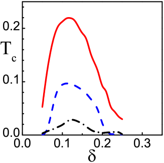
To compare various mechanisms of pairing, let us consider the solution of equation (4.3) for as a function of hole doping in the weak coupling approximation (WCA) neglecting the self-energy contribution by taking . In WCA we obtain high values for as shown in figure 1. A very high is found when all the contributions are taken into account. The spin-fluctuation pairing results in superconducting which is much larger than mediated only by EPI. The doping dependence of qualitatively agrees with experiments in cuprates but its value is too high. It is important to stress that contributions from CI and EPI are suppressed since they are given by component of the interactions. In particular, EPI may be strong for phonon modes with -independent interaction resulting in but providing a pronounced polaronic effect observed in experiments. Similar contribution from single-site CI is zero. We also note that the pairing in the MFA induced by the AF exchange proposed by Anderson [17] provides quite a low which is suppressed by the intersite CI since .
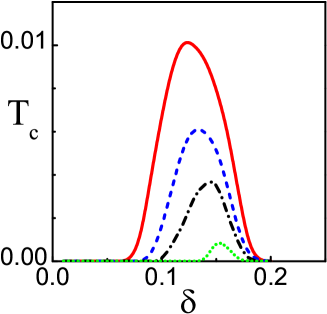
Now, we consider the solution of equation (4.2) taking into account the renormalization parameter which is quite large, , as shown in references [9, 10]. In this case we obtain the values of that are an order of magnitude smaller. Figure 2 shows the solution of equation (4.2) for in the presence of the intersite CI. for is quite high due to a strong coupling induced by the kinematical interaction and is close to experimentally observed one, K, for the characteristic value of eV. Increasing suppresses which becomes small only for high values of comparable with the spin-fluctuation coupling and is much larger than the EPI and the AF exchange interaction .
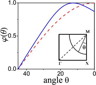
As discussed in [9, 10, 11], numerical solution of the full gap equation shows the energy gap dependence characteristic of the pairing induced by bosons, in our theory — spin-fluctuations. The -dependence of the gap function on the Fermi surface at doping shown in figure 3 reveals the -wave symmetry which angle dependence is close to the model -wave dependence .
By taking into account the electron-phonon interaction within the extended Hubbard model (3.1) the isotope effect (IE) was found [11]. The IE exponent is small, , at optimal doping, while in the underdoped region, the IE increases and can be even larger than in the conventional superconductors, , which is in a qualitative agreement with experiments.
5 Conclusion
The microscopic theory of superconductivity of strongly correlated electronic systems such as cuprates is formulated. The superconducting pairing is provided by strong kinematical interaction of electrons with spin excitations. The EPI and the intersite CI are suppressed for the -wave pairing since only symmetry components of the interactions give contributions. We emphasize that there is no kinematical interaction in the phenomenological spin-fermion models where the conventional electrons interacting with spin fluctuations are considered. The kinematical interaction is lost in the slave-boson (-fermion) models treated in the MFA where the projected electron operators are approximated by a product of conventional electron and boson operators in MFA: .
The spin-fluctuation mechanism was supported in many publications, in particular, for systems with strong electron correlations. Here, we refer to numerical simulations for finite clusters (see reviews [26, 29, 27, 30, 28]), the dynamical cluster approximation (DCA) [31, 32, 33], and the cluster dynamical mean-field theory (see, e.g., [34, 35, 36]). Extensive numerical studies for finite clusters have revealed a tendency to the -wave pairing in the Hubbard model at large , though a delicate balance between superconductivity and other instabilities (AF, spin-density wave, charge-density wave, etc.) was found in the above cited references. In [37], using the DCA with the quantum Monte Carlo method, the superconducting -wave pairing and the isotope effect similar to the one observed in cuprates were found for the Hubbard-Holstein model. However, in some finite cluster calculations, an appearance of the long-range superconducting order has not been confirmed (see, e.g., [38]). The drawback of this result may be due to a finite number of electrons in clusters.
Our conclusion concerning the importance of the kinematical mechanism of pairing is supported by the studies in [39]. Using the variational Monte Carlo technique the superconducting -wave gap was observed for the extended Hubbard model with a weak exchange interaction and a repulsion in a broad range of . It was found that the gap decreases with increasing at all and can be suppressed for for small . However, for large the gap becomes robust and exists up to large values of . We can give an explanation of these results by pointing out that at large , the concomitant decrease of the bandwidth results in the splitting of the Hubbard band into the upper and lower subbands, and the emerging kinematical interaction induces the -wave pairing in one Hubbard subband. In that case, the second subband for large gives a small contribution which results in the -independent pairing. This can be suppressed by the repulsion being only larger than the kinematical interaction, as in our analytical calculations, figure 2. This suggests that the spin-fluctuation pairing induced by kinematical interaction is the most probable mechanism of superconductivity in the Hubbard model in the limit of strong correlations.
References
- [1] Bednorz J.G., Müller K.A, Z. Phys. B: Condens. Matter, 1986, 64, 189, doi:10.1007/BF01303701.
- [2] Plakida N.M., High-Temperature Cuprate Superconductors, Springer Series in Solid-State Sciences, Vol. 166, Springer–Verlag, Berlin, 2010.
- [3] Fulde P., Electronic correlations in molecules and solids (third Ed.), Springer–Verlag, Berlin, 1995.
- [4] Avella A., Mancini F. (Eds.), Theoretical Methods for Strongly Correlated Systems, Springer Series in Solid–State Sciences, Vol. 171, Springer–Verlag, Heidelberg, 2011.
-
[5]
Vladimirov A.A., Ihle D., Plakida N.M.,
Phys. Rev. B, 2009, 80, 104425 (12 pages),
doi:10.1103/PhysRevB.80.104425. -
[6]
Vladimirov A.A., Ihle D.,
Plakida N.M., Phys. Rev. B, 2011, 83, 024411 (13 pages),
doi:10.1103/PhysRevB.83.024411. - [7] Plakida N.M., Oudovenko V.S., Phys. Rev. B, 1999, 59, 11949–11961, doi:10.1103/PhysRevB.59.11949.
- [8] Plakida N.M., Oudovenko V.S., J. Exp. Theor. Phys., 2007, 104, 230–244, doi:10.1134/S1063776107020082. [Zh. Eksp. Teor. Fiz., 2007, 131, 259-274 (in Russian)].
- [9] Plakida N.M., Oudovenko V.S., Eur. Phys. J. B, 2013, 86, 115 (15 pages), doi:10.1140/epjb/e2013-31157-6.
-
[10]
Plakida N.M., Oudovenko V.S.,
J. Exp. Theor. Phys., 2014, 119, No. 3, 554–566,
doi:10.1134/S1063776114080123. [Zh. Eksp. Teor. Fiz., 2014, 146, 631 (in Russian)]. - [11] Plakida N.M., Physica C, 2016, 531, 39–59, doi:10.1016/j.physc.2016.10.002.
-
[12]
Bogoliubov N. N., Tyablikov S.V., Sov. Phys. Dokl. 1959, 4, 604,
[Doklady AN SSSR, 1959, 126, 53
(in Russian)]. - [13] Zubarev D.N., Sov. Phys. Usp., 1960, 3, 320–345, doi:10.3367/UFNr.0071.196005c.0071 [Uspekhi Fiz. Nauk, 1960, 71, No. 1, 71–116, (in Russian), doi:10.3367/UFNr.0071.196005c.0071].
- [14] Hubbard J., Proc. R. Soc. London, Ser. A, 1963, 276, 276.
- [15] Hubbard J., Proc. R. Soc. London, Ser. A, 1965 285, 542.
- [16] Dyson F., Phys. Rev., 1956, 102, 1217, doi:10.1103/PhysRev.102.1217.
- [17] Anderson P.W., Science, 1987, 235, 1196–1198, doi:10.1126/science.235.4793.1196.
- [18] Zaitsev R.O., Ivanov V.A., Soviet Phys. Solid State, 1987, 29, 2554.
- [19] Zaitsev R.O., Ivanov V.A., Soviet Phys. Solid State, 1987, 29, 3111.
- [20] Zaitsev R.O., Ivanov V.A., Int. J. Mod. Phys. B, 1988, 5, 153.
- [21] Plakida N.M., Yushankhai V.Yu., Stasyuk I.V., Physica C, 1989, 160, 80, doi:10.1016/0921-4534(89)90456-5.
- [22] Yushankhai V.Yu., Plakida N.M., Kalinay P., Physica C, 1991, 174, 401, doi:10.1016/0921-4534(91)91576-P.
- [23] Plakida N.M., In: Theoretical Methods for Strongly Correlated Systems, Springer Series in Solid–State Sciences, Vol. 171, Avella A., Mancini F. (Eds.), Springer–Verlag, Heidelberg, 2011, Chapter 6, 173–202.
- [24] Mori H., Prog. Theor. Phys., 1965, 34, 399, doi:10.1143/PTP.34.399.
- [25] Plakida N.M., In High-Temperature Cuprate Superconductors, Springer Series in Solid-State Sciences, Vol. 166, Springer–Verlag, Berlin, 2010, Appendix.
- [26] Scalapino D.J., Phys. Rep., 1995, 250, 329.
- [27] Scalapino D.J., In: Handbook of High-Temperature Superconductivity. Theory and Experiment, J.R. Schrieffer and J.S. Brooks (Eds.), Springer-Verlag, New York, 2007, 495–526.
- [28] Scalapino D.J., Rev. Mod. Phys., 2012, 84, 1383, doi:10.1103/RevModPhys.84.1383.
- [29] Bulut N., Adv. Phys., 2002, 51, 1587, doi:0.1080/00018730210155142.
- [30] Sénéchal D., In: Theoretical Methods for Strongly Correlated Systems, Springer Series in Solid–State Sciences, Vol. 171, Avella A., Mancini F. (Eds.), Springer–Verlag, Heidelberg, 2011, Chapter 11.
-
[31]
Maier Th., Jarrel M., Pruschke Th.,
Hettler M.H., Rev. Mod. Phys., 2005, 77, 1027,
doi:10.1103/RevModPhys.77.1027. - [32] Maier Th., Jarrel M., Scalapino D.J., Phys. Rev. Lett., 2006, 96, 047005, doi:10.1103/PhysRevLett.96.047005;
- [33] Maier Th., Jarrel M., Scalapino D.J., Phys. Rev. B, 2006, 74, 094513, doi:10.1103/PhysRevB.74.094513.
- [34] Capone M., Kotliar G., Phys. Rev. B, 2006, 74, 054513, doi:10.1103/PhysRevB.74.054513.
- [35] Haule K., Kotliar G., Phys. Rev. B, 2007, 76, 104509, doi:10.1103/PhysRevB.76.104509.
- [36] Kancharla S. S., Kyung B., Sénéchal D., Civelli M., Capone M., Kotliar G., Tremblay A.-M.S., Phys. Rev. B, 2008, 77, 184516, doi:10.1103/PhysRevB.77.184516.
- [37] Macridin A., Jarrell M., Phys. Rev. B, 2009, 79, 104517, doi:10.1103/PhysRevB.79.104517.
- [38] Aimi T., Imada M., J. Phys. Soc. Jpn., 2007, 76, 13708, doi:10.1143/JPSJ.76.113708.
- [39] Plekhanov E., Sorella S., Fabrizio M., Phys. Rev. Lett., 2003, 90, 187004, doi:10.1103/PhysRevLett.90.187004.
Ukrainian \adddialect\l@ukrainian0 \l@ukrainian
Ìiêðîñêîïiчíà òåîðiÿ âèñîêîòåìïåðàòóðíî¿ íàäïðîâiäíîñòi â ñèëüíîñêîðåëüîâàíèõ åëåêòðîííèõ ñèñòåìàõ Ì. Ì. Ïëàêiäà
Îá’єäíàíèé iíñòèòóò ÿäåðíèõ äîñëiäæåíü, 141980 Äóáíà, Ðîñiÿ