On the Computational Properties of
Obviously Strategy-Proof Mechanisms

Abstract

“Does there exist a strategy-proof mechanism for choice rule $c$?” “Does there exist an obviously strategy-proof mechanism for $c$?” We find that these two problems are of similar complexity. When $c$ is represented as a payoff table, both problems can be decided in polynomial time. When $c$ is represented as a Boolean circuit, both problems are co-NP-complete.

1 Introduction

Classical mechanism design focuses on direct mechanisms, but there is strong empirical evidence that the extensive form of the mechanism affects the rate of optimal play. A growing body of laboratory experiments documents that human subjects make frequent mistakes in direct mechanisms, but not in equivalent extensive-form mechanisms (Kagel et al., 1987; Kagel and Levin, 2001; McGee and Levin, 2019; Zhang and Levin, 2020; Schneider and Porter, 2020; Bó and Hakimov, 2020a, b).

Which mechanisms are easy for human beings to understand? Some intuitively simple extensive-form mechanisms, such as ascending auctions or dynamic serial dictatorships, are obviously strategy-proof (Li, 2017). Obvious strategy-proofness requires that for any information set reachable under the truth-telling strategy, and for any deviation starting at that information set, every possible outcome under the deviation is no better than every possible outcome from truth-telling. This formalizes a cognitive limitation: A mechanism is obviously strategy-proof if and only if participants can detect that truth-telling is optimal without using contingent reasoning. Another interpretation of obviously strategy-proof mechanisms is that they provide incentives under weaker assumptions about the designer’s commitment power.

Obvious strategy-proofness depends on the extensive form of the mechanism. For instance, ascending auctions are obviously strategy-proof, but second-price auctions are not. This raises new obstacles for mechanism design. By the revelation principle, the question “does there exist a strategy-proof (SP) mechanism for choice rule $c$?” reduces to the question of whether the corresponding direct mechanism is strategy-proof (Gibbard, 1973; Myerson, 1979). By contrast, the question “does there exist an obviously strategy-proof (OSP) mechanism for choice rule $c$?” is about the entire class of extensive-form game trees, which is combinatorially complex.

Extensive-form mechanisms can be simpler for the agents, but are they much more complicated for the designer? There is a growing literature that studies which choice rules have OSP mechanisms, in settings such as school choice, object allocation, social choice with single-peaked preferences, and the division problem. Do these clean characterizations arise because of particular assumptions about preferences, or is there hidden structure that makes the problem tractable in general?

To address these questions, we study the computational complexity of designing SP and OSP mechanisms. As input, we have agents with private preferences (types) and a choice rule (a function from type profiles to outcomes). The SP decision problem is “Does there exist a SP mechanism for this choice rule?”, and similarly for the OSP decision problem. The complexity of a problem is the computation time required to correctly answer “yes” or “no”, as a function of the input size. This depends on the input language—with a more concise language, more time is required to decide the problem for a given input size.

We start by studying the SP and OSP decision problems under table inputs. That is, the agents’ preferences and the choice rule are represented as a table, which specifies the payoff of each type of each agent, at each reported type profile.

Table inputs are a natural yardstick, because strategy-proofness asserts a system of inequalities with rank linear in the table size. To decide if the direct mechanism is strategy-proof, it is sufficient to check all these inequalities, so the SP problem can be solved in polynomial time. By contrast, there are exponentially many extensive-form mechanisms for each choice rule, so to decide the OSP problem by brute-force search would take exponential time.

We prove that the OSP decision problem with table inputs can be solved in polynomial time. Moreover, we show that OSP mechanisms, when they exist, can be constructed in polynomial time.

Along the way, we discover a characterization of OSP-implementable choice rules that may be of independent interest. Given any choice rule, we define a corresponding obvious directed acyclic graph (O-dag). The root of the O-dag corresponds to the set of all type profiles. Each vertex of the O-dag corresponds to a set of type profiles with a product structure.

The directed edges of the O-dag correspond to inferences that we can make by asking ‘obvious’ questions. That is, for any two vertices $v$ and $v^{\prime}$, there is a directed edge from $v$ to $v^{\prime}$ if we can make an ‘obvious’ binary query to one agent about his type, such that the type profile lies in $v^{\prime}$ if and only if the type profile lies in $v$ and the agent’s answer is “yes”. A binary query is obvious if, given the choice rule and given that the type profile is in $v$, every possible outcome from lying is no better than every possible outcome from answering truthfully.

We show that a choice rule has an OSP mechanism if and only if its O-dag is nicely connected, meaning that every singleton vertex can be reached from the root. Hence, one way to solve the OSP decision problem is to construct the O-dag and check whether it is nicely connected. However, a brute force approach to this verification does not yield a polynomial-time algorithm, because the O-dag has a vertex set that grows exponentially with the number of types.

Instead, our algorithm detects whether the O-dag is nicely connected without explicitly constructing the entire O-dag. We define a greedy algorithm that starts from the root and searches for a path to each singleton vertex. Since the algorithm is greedy, it quickly either finds such a path or returns a failure. We then exploit the structure of the O-dag to prove that failure to greedily find a path implies that no path exists.

The greedy algorithm terminates in sub-quadratic time with respect to the input table size. For comparison, deciding the SP decision problem requires time linear in the table size.

To summarize, deciding whether there exists an OSP mechanism for a choice rule is equivalent to deciding whether the corresponding O-dag is nicely connected, which can be done in polynomial time by a greedy algorithm.

The greedy algorithm can also be used to construct OSP mechanisms in polynomial time when they exist. Specifically, the O-dag edges visited by the algorithm assemble to form the desired mechanism.

The preceding results indicate that the SP and OSP decision problems are of similar computational complexity—they are both in the complexity class P when the inputs are payoff tables. However, in many natural settings, choice rules and utility functions have special structure that permits a shorter description. If we consider a more concise input language, are the problems still of similar complexity?

So far, the table inputs we have considered cannot concisely describe settings with many agents, because the table size required to describe a choice rule grows exponentially in the number of agents. Many natural choice rules are anonymous, in the sense that one agent’s payoffs are not changed when we permute the types of the other agents. These can be described using anonymous table inputs that grow only polynomially in the number of agents. By adapting the greedy algorithm to anonymous table inputs, we show that the OSP problem can still be decided in polynomial time.

Now we consider the SP and OSP decision problems when the utility functions and the choice rule are represented by Boolean circuits, one for each function. Each circuit consists of input nodes that are fed through a network of logic gates to the output nodes. The size of a circuit is the number of logic gates.

Boolean circuits are a more concise input language than payoff tables. When choice rules and utility functions have a ‘well-behaved’ logical structure, then they can often be represented using a small number of logic gates, even if the resulting table of payoffs is quite large. Consequently, we should expect that (for a given input size) the time to decide both problems will increase under circuit inputs.

Our results for circuit inputs involve the complexity class co-NP. Roughly, this consists of problems such that whenever the answer is “no”, there exists a proof that can be quickly checked. Formally, a decision problem is in co-NP if for every no-instance there exists a polynomial-length certificate that can be verified by a polynomial-time algorithm. It is widely believed that the hardest problems in co-NP cannot be solved in polynomial time.

Boolean circuits are a very concise input language, so one may expect that the SP and OSP decision problems are hard with circuit inputs. We prove that both problems are co-NP-hard, that is, at least as hard as the hardest problems in co-NP. The proof proceeds by a reduction from Boolean satisfiability, a NP-hard decision problem. This result provides a lower bound for the complexity of deciding whether an SP (or OSP) mechanism exists for a given choice rule.

Next we establish upper bounds for the complexity of the SP and OSP problems. When a choice rule is not strategy-proof, this can be certified by presenting a type profile and a profitable deviation for one agent. Such a certificate can be checked in polynomial time, so the SP decision problem with circuit inputs is in co-NP.

Is the OSP problem with circuit inputs in co-NP? That is, when no OSP mechanism exists for a given choice rule, is there always a quick proof of non-existence? We prove this by exploiting the O-dag structure developed earlier. We find that there exists no OSP mechanism for a choice rule if and only if some non-singleton vertex of its O-dag has no children. Thus, one can certify the no-instances of the OSP problem by exhibiting such a vertex and proving that it has no children, which can be done in polynomial time.

The preceding results imply that the SP and OSP problems are co-NP-complete under circuit inputs. That is, they are as hard as, but no harder than, the hardest problems in co-NP. This implies that either problem can be reduced to the other in polynomial time.

In summary, our results indicate that it is similarly complex to decide whether a choice rule has a corresponding SP mechanism or OSP mechanism, despite the apparent hurdles introduced by considering extensive forms. With table inputs, one can decide the OSP problem and construct the mechanism in polynomial time. With circuit inputs, when the desired mechanism does not exist, there is always a short proof of the claim.

Computational constraints can be just as real as the constraints imposed by information or incentives. There is growing interest in how these constraints affect the design of economic systems (Mu’Alem and Nisan, 2008; Hartline and Lucier, 2015; Camara, 2021; Akbarpour et al., 2022). The present results suggest that making mechanisms simple for human participants does not come at a large cost in computational complexity for the designer.

2 Model and primitives

Consider a finite set of agents $N$ with type sets $T_{1},\dots,T_{n}$, and an outcome set $X$. We assume private values: each agent has a utility function $u_{i}:T_{i}\times X\rightarrow\mathbb{R}$. For each type $t_{i}$, let the binary relation $\succeq_{t_{i}}$ denote the weak preference ordering over outcomes induced by $t_{i}$, that is, $x\succeq_{t_{i}}x^{\prime}$ if $u_{i}(t_{i},x)\geq u_{i}(t_{i},x^{\prime})$. Let $T\equiv T_{1}\times\cdots\times T_{n}$, with representative element $t$.

A choice rule is a function $c:T\rightarrow X$. As usual, we use $T_{-i}$ to denote $\prod_{j\in N\setminus\{i\}}T_{j}$, and $t_{-i}$ to denote an element of $T_{-i}$. We use analogous notation for products of subsets of the type sets.

Definition 1.

Choice rule $c$ is strategy-proof (SP) if for all $t_{i}$, $t^{\prime}_{i}$, and $t_{-i}$,

$$c(t_{i},t_{-i})\succeq_{t_{i}}c(t^{\prime}_{i},t_{-i}).$$ (1)

2.1 Definition of extensive-form mechanisms

Informally, a mechanism is an extensive game form for which each terminal history is associated with some outcome. In principle, such a mechanism could have imperfect information or even imperfect recall. Furthermore, agents could in principle play mixed strategies or behavioral strategies. However, for our purposes it is without loss of generality to restrict attention to mechanisms in which agents take turns to make public announcements about their private information, and play pure strategies (Mackenzie, 2020). To ease notation, we restrict attention to this class, which was identified by Ashlagi and Gonczarowski (2018), and refined by Pycia and Troyan (2021), Bade and Gonczarowski (2017), and Mackenzie (2020). We additionally restrict attention to mechanisms in which every type profile results in a finite play.

Formally, given a choice rule $c$, a mechanism for $c$ specifies a directed rooted tree with vertex set $V$ and edge set $E$. Essentially, we start play from the root vertex $\overline{v}$, and at each step one agent makes a declaration about his type. We use $\text{out}(v)$ to denote the out-edges of vertex $v$, and $Z$ to denote the terminal vertices, i.e. those with no out-edges. For each non-terminal vertex $v$, some agent is called to play, whom we denote $P(v)$. Figure 1 illustrates such a mechanism.

Each vertex $v\in V$ is associated with a set of types $T_{i}^{v}\subseteq T_{i}$ for each agent $i$, and we denote $T^{v}=\prod_{i}T_{i}^{v}$. We interpret the out-edges as reports that could be made by $P(v)$. Hence, for any non-terminal vertex $v$, each edge $e\in\text{out}(v)$ corresponds to a non-empty subset of $P(v)$’s types, denoted $T_{P(v)}^{e}$. We require that the family of sets $(T_{P(v)}^{e})_{e\in\text{out}(v)}$ is a partition of $T_{P(v)}^{v}$.

We interpret $T_{i}^{v}$ as the types of $i$ consistent with the reports so far, which requires some record-keeping. Hence we require that at the root vertex all types are possible, $T^{\overline{v}}=T$. We also require that if $v^{\prime}$ is child of $v$ reached by edge $e$, then $T_{P(v)}^{v^{\prime}}=T_{P(v)}^{e}$ and for all $i\neq P(v)$, $T_{i}^{v^{\prime}}=T_{i}^{v}$.

We require that every type profile results in a finite play; that is, for all $t\in T$, there exists a terminal vertex $v\in Z$ such that $t\in T^{v}$. This implies that the terminal vertices $Z$ induce a partition of $T$, which is $(T^{v})_{v\in Z}$.

Finally, we require that the reports yield enough information to enact the choice rule. Formally, this means that the choice rule $c$ is measurable with respect to the partition induced by the terminal vertices, i.e. for all $v\in Z$ and all $t,t^{\prime}\in T^{v}$, $c(t)=c(t^{\prime})$.

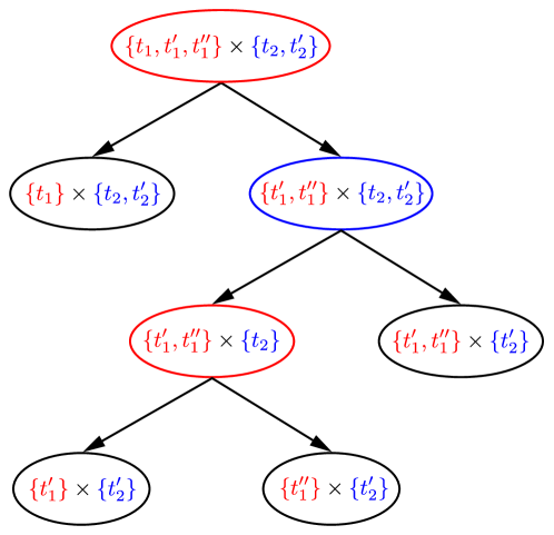
Figure 1: Example of a mechanism. Agent $1$ plays at the red vertices, agent $2$ plays at the blue vertex, and the other vertices are terminal.

2.2 Obvious strategy-proofness

Given some non-terminal vertex $v$, we say that $t_{P(v)}$ and $t^{\prime}_{P(v)}$ diverge at $v$ if $t_{P(v)},t^{\prime}_{P(v)}\in T_{P(v)}^{v}$ and they make distinct reports, that is, if there is no $e\in\text{out}(v)$ such that $t_{P(v)},t^{\prime}_{P(v)}\in T_{P(v)}^{e}$.

Definition 2.

A mechanism for $c$ is obviously strategy-proof (OSP) if for any agent $i$, any vertex $v$ with $P(v)=i$, any $t_{i}$ and $t^{\prime}_{i}$ that diverge at $v$, and any $t_{-i},t^{\prime}_{-i}\in T_{-i}^{v}$, we have that

$$c(t_{i},t_{-i})\succeq_{t_{i}}c(t^{\prime}_{i},t^{\prime}_{-i}).$$ (2)

We say that $c$ is OSP-implementable if there exists an OSP mechanism for $c$.

We will also sometimes use the following intuitive terminology. By definition, each vertex $v$ has the associated query $(P(v),T^{v},\{T_{P(v)}^{e}\}_{e\in\text{out}(v)})$ that asks player $P(v)$ which partition element $T_{P(v)}^{e}$ contains their type, given that the overall type profile lies in $T^{v}$. We say this query is obvious if (2) holds for any $t_{i}$ and $t_{i}^{\prime}$ that diverge at $v$, and any $t_{-i},t^{\prime}_{-i}\in T_{-i}^{v}$. Then a mechanism is OSP if and only if the query at every vertex is obvious.

We now contrast Definition 1 and Definition 2. Definition 1 is a state-by-state comparison; for any $t_{-i}$, type $t_{i}$ must prefer truthful reporting to any deviation. By contrast, Definition 2 compares every possible outcome following the truthful report to every possible outcome following a deviation, but restricts this comparison to vertices at which play diverges. This property depends on the extensive form of the mechanism.

Definition 2 is a stronger requirement than Definition 1. For any choice rule $c$, if $c$ is OSP-implementable, then $c$ is SP.

The original definition of OSP restricts attention to mechanisms with a uniform bound on the depth of the game tree (Li, 2017). Here we have only made the weaker requirement that every type profile results in a finite play. Definition 2 is equivalent to the original definition on game trees with a uniform bound. Were we to make this additional restriction, we would need to strengthen the connectedness requirement (Definition 4), but it would not otherwise alter any of the results.

3 A characterization of OSP-implementable choice rules

For any given choice rule $c$, the number of mechanisms for $c$ is exponential in $|T_{i}|$ for each agent $i$. In this section, we develop a machinery that associates each choice rule with a single directed acyclic graph. We then prove that there exists an OSP mechanism for $c$ if and only if the graph is connected in a particular way.

Definition 3.

The obvious directed acyclic graph (O-dag) of choice rule $c$ is the directed acyclic graph with vertex set

$$\left\{\prod_{i}T_{i}^{\prime}\ \middle|\ \forall i:\emptyset\subset T_{i}^{\prime}\subseteq T_{i}\right\}$$ (3)

and with edge set containing all edges of the form

$$T^{\prime}\Rightarrow(A_{i},T^{\prime}_{-i})$$ (4)

where $\emptyset\subset A_{i}\subset T_{i}^{\prime}$, such that for all $a_{i}\in A_{i}$, all $a^{\prime}_{i}\in T_{i}^{\prime}\setminus A_{i}$, and all $t_{-i},t^{\prime}_{-i}\in T^{\prime}_{-i}$

$$c(a_{i},t_{-i})\succeq_{a_{i}}c(a^{\prime}_{i},t^{\prime}_{-i})\text{ and }c(a^{\prime}_{i},t^{\prime}_{-i})\succeq_{a^{\prime}_{i}}c(a_{i},t_{-i}).$$ (5)

The similarity between the inequalities in Definition 2 and Definition 3 can be explained as follows: The O-dag contains exactly those edges $T^{\prime}\Rightarrow(A_{i},T_{-i}^{\prime})$ for which the binary query $(i,T^{\prime},\{A_{i},T_{i}^{\prime}\setminus A_{i}\})$ asking whether agent $i$’s type lies in $A_{i}$ or $T_{i}^{\prime}\setminus A_{i}$ is obvious (see Section 2.2).

Definition 4.

The O-dag of $c$ is nicely connected if for every $t\in T$, there exists a path from the root $T$ to the vertex $\{t\}$.

The main result of this section, stated below, shows that OSP-implementable choice rules are characterized by this connectedness property. This enables us to reduce a question about the class of all mechanisms for $c$ to a question about the O-dag of $c$.

Theorem 1.

For any choice rule $c$, there exists an OSP mechanism for $c$ if and only if the O-dag of $c$ is nicely connected.

In subsequent sections, we will use the O-dag characterization to answer algorithmic questions about OSP mechanisms. However, the characterization may be of independent interest. For instance, Lemma 2 below and Theorem 1 together yield a tractable method to prove the non-existence of OSP mechanisms for particular choice rules, stated in the following corollary.

Corollary 1.

For any choice rule $c$, if the O-dag of $c$ contains a non-singleton vertex $T^{\prime}$, and $t\in T^{\prime}$ such that there is no path from $T^{\prime}$ to $\{t\}$, then $c$ is not OSP-implementable.

When type spaces are finite, all paths in the O-dag are finite. This property gives the stronger condition below.

Corollary 2.

If all $T_{i}$ are finite, then a choice rule $c$ is OSP-implementable if and only if every non-singleton vertex in its O-dag has a child.

Proof.

If the O-dag of $c$ contains a non-singleton vertex with no child, then Corollary 1 implies that $c$ is not OSP-implementable.

For the converse, let every non-singleton vertex of the O-dag have a child. Consider any $t\in T$. Inductively construct a path $T^{1},T^{2},\dots$ with $T^{1}=T$ such that $T^{k+1}$ is any child of $T^{k}$ that contains $t$. The path ends upon reaching some $T^{K}$ with no such child. If $T^{K}$ were non-singleton, then it would have some children $(A_{i},T_{-i}^{K})$ and $(T_{i}^{K}\setminus A_{i},T_{-i}^{K})$, one of which contains $t$, a contradiction. Thus $T^{K}=\{t\}$. Therefore the O-dag is nicely connected, so $c$ is OSP-implementable by Theorem 1. ∎

We now turn to proving Theorem 1. To begin, we establish some properties of the O-dag that aid in the characterization. The following lemma shows that each edge in the O-dag implies the existence of all edges obtained by passing to restricted type sets. That is, an obvious binary query remains obvious upon restricting the set of possible types.

Lemma 1.

If the O-dag of $c$ contains an edge $T^{\prime}\Rightarrow(A_{i},T^{\prime}_{-i})$, then for any vertex $B\subseteq T^{\prime}$ such that $\emptyset\subset(A_{i}\cap B_{i})\subset B_{i}$, the O-dag of $c$ also contains the edge $B\Rightarrow(A_{i}\cap B_{i},B_{-i})$.

Proof.

Take any $a_{i}\in A_{i}\cap B_{i}$, any $a^{\prime}_{i}\in B_{i}\setminus(A_{i}\cap B_{i})$, and any $t_{-i},t^{\prime}_{-i}\in B_{-i}$. Observe that $A_{i}\cap B_{i}\subseteq A_{i}$, $B_{i}\setminus(A_{i}\cap B_{i})\subseteq T^{\prime}_{i}\setminus A_{i}$, and $B_{-i}\subseteq T^{\prime}_{-i}$. Since the O-dag of $c$ contains $T^{\prime}\Rightarrow(A_{i},T^{\prime}_{-i})$, we have that

$$c(a_{i},t_{-i})\succeq_{a_{i}}c(a^{\prime}_{i},t^{\prime}_{-i})\text{ and }c(a^{\prime}_{i},t^{\prime}_{-i})\succeq_{a^{\prime}_{i}}c(a_{i},t_{-i}).$$ (6)

Hence, the O-dag of $c$ contains the edge $B\Rightarrow(A_{i}\cap B_{i},B_{-i})$. ∎

To ease notation, note that the Cartesian product is distributive over intersections, so for any two sets $A=\prod_{i}A_{i}$ and $B=\prod_{i}B_{i}$ we have $A\cap B=\prod_{i}\left(A_{i}\cap B_{i}\right)$.

Below, we iteratively apply Lemma 1 to show that each path in the O-dag implies the existence of all paths obtained by passing to restricted type sets.

Lemma 2.

If the O-dag of $c$ contains a path from vertex $T^{\prime}$ to vertex $T^{\prime\prime}$, then for any vertex $B$ such that $B_{i}\cap T^{\prime\prime}_{i}\neq\emptyset$ for all $i$, the O-dag contains a path from $B\cap T^{\prime}$ to $B\cap T^{\prime\prime}$.

Proof.

Let $T^{1},T^{2},\ldots,T^{K}$ be a path with $T^{1}=T^{\prime}$ and $T^{K}=T^{\prime\prime}$. By construction, for all $k<K$ we have an edge $T^{k}\Rightarrow T^{k+1}$ and for some agent $i$, $T^{k+1}=(T_{i}^{k+1},T_{-i}^{k})$ and $\emptyset\subset T_{i}^{k+1}\subset T_{i}^{k}$.

Suppose $B_{i}\cap T_{i}^{k}\supset B_{i}\cap T_{i}^{k+1}$. Observe that $B_{i}\cap T_{i}^{k+1}\supseteq B_{i}\cap T^{\prime\prime}_{i}\neq\emptyset$. Then by Lemma 1, the O-dag contains the edge $B\cap T^{k}\Rightarrow B\cap T^{k+1}$.

Suppose $B_{i}\cap T_{i}^{k}=B_{i}\cap T_{i}^{k+1}$. Then, by $T_{-i}^{k}=T_{-i}^{k+1}$, we have that $B\cap T^{k}=B\cap T^{k+1}$.

Hence, for all $k<K$, either there exists an edge $B\cap T^{k}\Rightarrow B\cap T^{k+1}$ or $B\cap T^{k}=B\cap T^{k+1}$, so there exists a path from $B\cap T^{\prime}$ to $B\cap T^{\prime\prime}$. ∎

We now introduce notation for the ‘answers’ that are feasible from a vertex $T^{\prime}$ of the O-dag, which are precisely the possible answers to obvious queries at $T^{\prime}$. For any vertex $T^{\prime}$ in the O-dag of $c$, let $\mathcal{A}_{i}(T^{\prime})$ denote the family of sets

$$\left\{A_{i}\ \middle|\ \text{the O-dag contains $T^{\prime}\Rightarrow(A_{i},T^{\prime}_{-i}))$}\right\}.$$ (7)

The symmetry of Definition 3 implies that $\mathcal{A}_{i}(T^{\prime})$ is closed under complements (relative to $T^{\prime}_{i}$). We now prove that it is closed under intersections and unions.

Lemma 3.

Let $T^{\prime}$ be any vertex of the O-dag of $c$. For any agent $i$, consider some indexed sub-family $\{A_{i}^{k}\mid k\in K\}\subseteq\mathcal{A}_{i}(T^{\prime})$ with at least one member.

1. If $\emptyset\subset\bigcap_{k}A_{i}^{k}$, then $\bigcap_{k}A_{i}^{k}\in\mathcal{A}_{i}(T^{\prime})$.

2. If $\bigcup_{k}A_{i}^{k}\subset T^{\prime}_{i}$, then $\bigcup_{k}A_{i}^{k}\in\mathcal{A}_{i}(T^{\prime})$.

Proof.

Suppose the antecedent of Clause 1, $\emptyset\subset\bigcap_{k}A_{i}^{k}$. By Definition 3, we have $\bigcap_{k}A_{i}^{k}\subset T^{\prime}_{i}$. Take any $t_{i}\in\bigcap_{k}A_{i}^{k}$. For all $k$, $A_{i}^{k}\in\mathcal{A}_{i}(T^{\prime})$. Thus, for all $t^{\prime}_{i}\in\bigcup_{k}(T^{\prime}_{i}\setminus A_{i}^{k})$, we have

$$\forall t_{-i},t^{\prime}_{-i}\in T^{\prime}_{-i}:c(t_{i},t_{-i})\succeq_{t_{i}}c(t^{\prime}_{i},t^{\prime}_{-i})$$ (8)

$$\forall t_{-i},t^{\prime}_{-i}\in T^{\prime}_{-i}:c(t^{\prime}_{i},t^{\prime}_{-i})\succeq_{t^{\prime}_{i}}c(t_{i},t_{-i}).$$ (9)

Moreover, $\bigcup_{k}(T^{\prime}_{i}\setminus A_{i}^{k})=T^{\prime}_{i}\setminus\bigcap_{k}A_{i}^{k}$, so $\bigcap_{k}A_{i}^{k}\in\mathcal{A}_{i}(T^{\prime})$. This proves Clause 1 of Lemma 3.

Suppose the antecedent of Clause 2, $\bigcup_{k}A_{i}^{k}\subset T^{\prime}_{i}$. Note that $T^{\prime}_{i}\setminus\bigcup_{k}A_{i}^{k}=\bigcap_{k}(T^{\prime}_{i}\setminus A_{i}^{k})$, so we have

$$\emptyset\subset\bigcap_{k}(T^{\prime}_{i}\setminus A_{i}^{k}).$$ (10)

For all $k$, $A_{i}^{k}\in\mathcal{A}_{i}(T^{\prime})$, so by closure under relative complement we have that for all $k$,

$$T^{\prime}_{i}\setminus A_{i}^{k}\in\mathcal{A}_{i}(T^{\prime}).$$ (11)

By Clause 1, (10), and (11), we have that

$$\bigcap_{k}(T^{\prime}_{i}\setminus A_{i}^{k})\in\mathcal{A}_{i}(T^{\prime}).$$ (12)

Substituting $\bigcap_{k}(T^{\prime}_{i}\setminus A_{i}^{k})=T^{\prime}_{i}\setminus\bigcup_{k}A_{i}^{k}$ in (12) and applying closure under relative complement yields $\bigcup_{k}A_{i}^{k}\in\mathcal{A}_{i}(T^{\prime})$, which proves Clause 2 of Lemma 3. ∎

These observations imply there exists a partition of $T_{i}^{\prime}$ that contains all minimal elements of $\mathcal{A}_{i}(T^{\prime})$. This partition provides the most fine-grained set of answers of any obvious query for agent $i$ at vertex $T^{\prime}$. We formalize this idea below.

Lemma 4.

Let $T^{\prime}$ be any vertex in the O-dag of $c$. For any $i$, if $\mathcal{A}_{i}(T^{\prime})$ is non-empty, then there exists a partition $\overline{\mathcal{A}}_{i}(T^{\prime})$ of $T^{\prime}_{i}$ such that:

1. $\overline{\mathcal{A}}_{i}(T^{\prime})\subseteq\mathcal{A}_{i}(T^{\prime})$

2. For any $A_{i}\in\mathcal{A}_{i}(T^{\prime})$ and any $t_{i}\in A_{i}$, the unique element $A^{\prime}_{i}\in\overline{\mathcal{A}}_{i}(T^{\prime})$ such that $t_{i}\in A^{\prime}_{i}$ satisfies $A^{\prime}_{i}\subseteq A_{i}$.

Proof.

For any $t_{i}\in T^{\prime}_{i}$, let us define

$$\mathcal{A}_{i}(t_{i},T^{\prime})\equiv\left\{A_{i}\in\mathcal{A}_{i}(T^{\prime})\ \middle|\ t_{i}\in A_{i}\right\}.$$ (13)

Note that by $\mathcal{A}_{i}(T^{\prime})$ non-empty, there exists at least one element $A^{\prime}_{i}\in\mathcal{A}_{i}(T^{\prime})$. By closure under relative complement, we have $T^{\prime}_{i}\setminus A^{\prime}_{i}\in\mathcal{A}_{i}(T^{\prime})$. Hence, for all $t_{i}\in T^{\prime}_{i}$, $\mathcal{A}_{i}(t_{i},T^{\prime})$ is non-empty. Now we define

$$\overline{\mathcal{A}}_{i}(T^{\prime})\equiv\left\{\bigcap\mathcal{A}_{i}(t_{i},T^{\prime})\ \middle|\ t_{i}\in T^{\prime}_{i}\right\}.$$ (14)

Observe that for all $t_{i}\in T^{\prime}_{i}$, we have $t_{i}\in\bigcap\mathcal{A}_{i}(t_{i},T^{\prime})$, which implies that $\bigcup\overline{\mathcal{A}}_{i}(T^{\prime})=T^{\prime}$.

Next we prove Clause 1 of Lemma 4. Take any $t_{i}\in T^{\prime}_{i}$. By construction $\emptyset\subset\{t_{i}\}\subseteq\bigcap\mathcal{A}_{i}(t_{i},T^{\prime})$. By Lemma 3, $\bigcap\mathcal{A}_{i}(t_{i},T^{\prime})\in\mathcal{A}_{i}(T^{\prime})$. And $t_{i}$ was chosen arbitrarily, so we have that $\overline{\mathcal{A}}_{i}(T^{\prime})\subseteq\mathcal{A}_{i}(T^{\prime})$, which proves Clause 1.

Now we prove that any two elements of $\overline{\mathcal{A}}_{i}(T^{\prime})$ are either disjoint or identical. Take any $A_{i},A^{\prime}_{i}\in\overline{\mathcal{A}}_{i}(T^{\prime})$. By Clause 1, $A_{i},A^{\prime}_{i}\in\mathcal{A}_{i}(T^{\prime})$. By construction, there exists $t_{i}$ such that $A_{i}=\bigcap\mathcal{A}_{i}(t_{i},T^{\prime})$. Either $t_{i}\in A^{\prime}_{i}$ or $t_{i}\in T^{\prime}_{i}\setminus A^{\prime}_{i}$.

Suppose $t_{i}\in A^{\prime}_{i}$. By Lemma 3, $A_{i}\cap A^{\prime}_{i}\in\mathcal{A}_{i}(T^{\prime})$, so $A_{i}\cap A^{\prime}_{i}\in\mathcal{A}_{i}(t_{i},T^{\prime})$, which yields $A_{i}=\bigcap\mathcal{A}_{i}(t_{i},T^{\prime})\subseteq A_{i}\cap A^{\prime}_{i}\subseteq A^{\prime}_{i}$.

Suppose $t_{i}\in T^{\prime}_{i}\setminus A^{\prime}_{i}$. By closure under relative complement, $T^{\prime}_{i}\setminus A^{\prime}_{i}\in\mathcal{A}_{i}(T^{\prime})$. By Lemma 3, $A_{i}\cap(T^{\prime}_{i}\setminus A^{\prime}_{i})\in\mathcal{A}_{i}(T^{\prime})$, so $A_{i}\cap(T^{\prime}_{i}\setminus A^{\prime}_{i})\in\mathcal{A}_{i}(t_{i},T^{\prime})$. Thus, we have $A_{i}=\bigcap\mathcal{A}_{i}(t_{i},T^{\prime})\subseteq A_{i}\cap(T^{\prime}_{i}\setminus A^{\prime}_{i})\subseteq T^{\prime}_{i}\setminus A^{\prime}_{i}$. This implies that $A_{i}\cap A^{\prime}_{i}=\emptyset$.

We have proved that either $A_{i}\cap A^{\prime}_{i}=\emptyset$ or $A_{i}\subseteq A^{\prime}_{i}$. By symmetry, we also have that $A_{i}\cap A^{\prime}_{i}=\emptyset$ or $A_{i}\supseteq A^{\prime}_{i}$. Thus, $A_{i}$ and $A^{\prime}_{i}$ are either disjoint or identical. We have established that $\overline{\mathcal{A}}_{i}(T^{\prime})$ is a partition of $T^{\prime}$.

Clause 2 follows by construction of $\overline{\mathcal{A}}_{i}(T^{\prime})$. Observe that for any $A_{i}\in\mathcal{A}_{i}(T^{\prime})$ and any $t_{i}\in A_{i}$, we have that $A_{i}\in\mathcal{A}_{i}(t_{i},T^{\prime})$. So for $A^{\prime}_{i}=\bigcap\mathcal{A}_{i}(t_{i},T^{\prime})$, we have that $A^{\prime}_{i}\subseteq A_{i}$, which completes the proof. ∎

We are now ready to prove Theorem 1.

Proof of Theorem 1.

Suppose there exists an OSP mechanism for $c$, and denote its vertex set $V$ and its edge set $E$. Take any $t\in T$. There exists a terminal vertex $z$ such that $t\in T^{z}$. Hence there exists a path $v^{1},v^{2},\ldots,v^{K}$ in the tree such that $\overline{v}=v^{1}$ and $v^{K}=z$.

We now prove that for all $k<K$, the O-dag of $c$ contains the edge $T^{v^{k}}\Rightarrow T^{v^{k+1}}$. Let $i=P(v^{k})$. By construction, $\emptyset\subset T_{i}^{v^{k+1}}\subset T_{i}^{v^{k}}$ and $T_{-i}^{v^{k+1}}=T_{-i}^{v^{k}}$. Take any $t_{i}\in T_{i}^{v^{k+1}}$ and any $t^{\prime}_{i}\in T_{i}^{v^{k}}\setminus T_{i}^{v^{k+1}}$. Since $t_{i}$ and $t^{\prime}_{i}$ diverge at $v^{k}$ and the mechanism is OSP, it follows that for any $t_{-i},t^{\prime}_{-i}\in T_{-i}^{v^{k}}$,

$$c(t_{i},t_{-i})\succeq_{t_{i}}c(t^{\prime}_{i},t^{\prime}_{-i}).$$ (15)

Symmetry of Definition 2 implies that

$$c(t^{\prime}_{i},t^{\prime}_{-i})\succeq_{t^{\prime}_{i}}c(t_{i},t_{-i}).$$ (16)

which proves that the O-dag of $c$ contains the edge $T^{v^{k}}\Rightarrow T^{v^{k+1}}$.

Since $c$ is measurable with respect to the terminal vertices of the mechanism, we have that for all $t^{\prime},t^{\prime\prime}\in T^{v^{K}}$, $c(t^{\prime})=c(t^{\prime\prime})$. This implies that if $T^{v^{K}}\neq\{t\}$, then the O-dag contains the edge $T^{v^{K}}\Rightarrow\{t\}$. Thus, for all $t$, the O-dag of $c$ has a path from the root $T$ to $\{t\}$. This proves that if there exists an OSP mechanism for $c$, then the O-dag of $c$ is nicely connected.

Suppose that the O-dag of $c$ is nicely connected. We now construct an OSP mechanism for $c$. Essentially, we cycle through the bidders in a fixed order, keeping track of the type profiles consistent with all previous reports, $\tilde{T}^{k}$. At the $k$th step, we ask bidder $i$ to report a cell of the minimal partition $\overline{\mathcal{A}}_{i}(\tilde{T}^{k})$ if it is non-empty. Otherwise, we skip bidder $i$. The key is to show that the O-dag being nicely connected implies that this procedure does not get stuck for any type profile.

Formally, we generate the mechanism using the following procedure: As before, we identify agents with integers $1,\ldots,n$. Let $i^{k}\equiv(k\mod n)+1$. We initialize $\tilde{T}^{0}=T$. For $k=0,1,2,\ldots$, if $\mathcal{A}_{i^{k}}(\tilde{T}^{k})$ is non-empty, then $i^{k}$ reports $A_{i^{k}}\in\overline{\mathcal{A}}_{i^{k}}(\tilde{T}^{k})$ such that $t_{i^{k}}\in A_{i^{k}}$, which is well-defined and unique by Lemma 4. We then define $\tilde{T}^{k+1}\equiv(A_{i^{k}},\tilde{T}_{-i^{k}}^{k})$. If $\mathcal{A}_{i^{k}}(\tilde{T}^{k})$ is empty, we define $\tilde{T}^{k+1}\equiv\tilde{T}^{k}$. The procedure terminates if $\tilde{T}^{k}$ is singleton.

We now prove that the above procedure generates a mechanism for $c$. In particular, we show that for any $t\in T$, there is a terminal vertex $v$ of the mechanism such that $T^{v}=\{t\}$, which implies that every type profile results in a finite play, and also that the choice rule is measurable with respect to the partition induced by the terminal vertices.

Take any $t\in T$. Since the O-dag is nicely connected, there exists a path in the O-dag from $T$ to $\{t\}$, which we denote $T^{0},T^{1},\ldots,T^{K}$. Consider the sequence generated by the procedure when the type profile is $t$, which we denote $(\tilde{T}_{k})_{k=1}^{\infty}$. For convenience, if the procedure terminates at step $\tilde{K}$, we define $\tilde{T}^{k}=\tilde{T}^{\tilde{K}}$ for $k>\tilde{K}$.

We prove by induction that $\tilde{T}^{nk}\subseteq T^{k}$ for all $k\leq K$. The inductive hypothesis holds for $k=0$, since $\tilde{T}^{0}=T=T^{0}$. Suppose it holds for some $k<K$; we now prove it holds for $k+1$. Since $T^{0},T^{1},\ldots,T^{K}$ is a path in the O-dag, there exists some agent $j$ and some $A_{j}\subset T_{j}^{k}$ such that $(A_{j},T_{-j}^{k})=T^{k+1}$, and the O-dag contains edge

$$T_{j}^{k}\Rightarrow(A_{j},T_{-j}^{k})$$ (17)

If $\tilde{T}_{j}^{nk}\subseteq A_{j}$, then $\tilde{T}^{n(k+1)}\subseteq\tilde{T}^{nk}\subseteq(A_{j},T_{-j}^{k})=T^{k+1}$ and we are done. Suppose not, so $A_{j}\cap\tilde{T}_{j}^{nk}\subset\tilde{T}_{j}^{nk}$. Observe that $t\in A_{j}\cap\tilde{T}_{j}^{nk}$, so we have that

$$\emptyset\subset A_{j}\cap\tilde{T}_{j}^{nk}\subset\tilde{T}_{j}^{nk}.$$ (18)

$i^{l}=j$ for some $l$ weakly between $nk$ and $n(k+1)-1$, and $\tilde{T}_{j}^{l}=\tilde{T}_{j}^{nk}$. By construction and then by the inductive hypothesis,

$$\tilde{T}^{l}\subseteq\tilde{T}^{nk}\subseteq T^{k}.$$ (19)

By (17), (18), (19), and Lemma 1, the O-dag contains the edge

$$\tilde{T}^{l}\Rightarrow(A_{j}\cap\tilde{T}_{j}^{l},\tilde{T}^{l}_{-j}).$$ (20)

Since $\overline{\mathcal{A}}_{j}(\tilde{T}^{l})$ consists of the minimal elements of $\mathcal{A}_{j}(\tilde{T}^{l})$, (20) and the definition of the sequence imply that

$$\tilde{T}_{j}^{l+1}\subseteq A_{j}\cap\tilde{T}_{j}^{l}.$$ (21)

Hence,

$$\tilde{T}^{n(k+1)}\subseteq\tilde{T}^{l+1}\subseteq(A_{j}\cap\tilde{T}_{j}^{l},\tilde{T}_{-j}^{nk})\subseteq(A_{j},T_{-j}^{k})=T^{k+1}$$ (22)

which proves the inductive step. Thus, for all $k\leq K$, we have that $\tilde{T}^{nk}\subseteq T^{k}$. In particular, $\tilde{T}^{nK}\subseteq T^{K}=\{t\}$, so the procedure terminates after no more than $nK$ steps.

Consequently, for every type profile $t$, there exists a terminal vertex $v$ in the corresponding mechanism such that $T^{v}=\{t\}$, so the procedure generates a mechanism for $c$.

Finally, the mechanism generated by the procedure is OSP. In particular, if $t_{i}$ and $t^{\prime}_{i}$ diverge at some vertex $v$ of the mechanism, then $t_{i}$ and $t^{\prime}_{i}$ are in distinct cells of $\overline{\mathcal{A}}_{i}(T^{v})$. Hence, we have that for any $t_{-i},t^{\prime}_{-i}\in T_{-i}^{v}$,

$$c(t_{i},t_{-i})\succeq_{t_{i}}c(t^{\prime}_{i},t^{\prime}_{-i}).$$ (23)

Thus, if the O-dag of $c$ is nicely connected, then there exists an OSP mechanism for $c$. ∎

4 An algorithm for deciding whether a choice rule is OSP-implementable

This section studies the computational problem of determining whether a choice rule is OSP-implementable, assuming finite type spaces. For an arbitrary choice rule $c$, we use the structure of the O-dag of $c$ to efficiently determine if $c$ is OSP-implementable.

Suppose we have finite type sets $(T_{i})_{i\in N}$, outcome set $X$, a choice rule $c:\prod_{i}T_{i}\rightarrow X$, and utility functions $u_{i}:T_{i}\times X\rightarrow\mathbb{R}$. An instance of the decision problem is comprised by $\sum_{i}|T_{i}|$ functions, one for each type $t_{i}$,

$$u_{i}(t_{i},\cdot)\circ c:T_{1}\times\cdots\times T_{n}\rightarrow\mathbb{R}.$$ (24)

Each of these functions requires $\prod_{i}|T_{i}|$ real numbers to express in general. In our decision problem, we take these functions as the input. Hence, we define

$$|c|=\left(\sum_{i}|T_{i}|\right)\prod_{i}|T_{i}|$$ (25)

which is the size of the table that specifies the payoffs to each type of each agent, for each profile of reports. Running times for algorithms on $c$ will be expressed as a function of $|c|$.

First consider the problem of deciding whether $c$ is strategy-proof. For each $i$ and each $t_{i}\in T_{i}$, it is necessary and sufficient to verify for all $t_{i}^{\prime}\in T_{i}$ and all $t_{-i}\in T_{-i}$ that $u_{t_{i}}(c(t_{i},t_{-i}))\geq u_{t_{i}}(c(t_{i}^{\prime},t_{-i}))$. This verification requires $\sum_{i}|T_{i}|^{2}|T_{-i}|=|c|$ steps, so deciding whether $c$ is SP requires linear time.

The following result states that it is not much more difficult to determine if $c$ is OSP-implementable.

Theorem 2.

There exists a $O(|c|\sum_{i}|T_{i}|)$-time algorithm for deciding whether $c$ is OSP-implementable.

To put this result in context, consider that while the number of histories in an arbitrary OSP mechanism for $c$ may grow exponentially in $|c|$, the gradual revelation principle of Bade and Gonczarowski (2017) guarantees that every OSP mechanism for $c$ has an OSP implementation of depth at most $\sum_{i}|T_{i}|$ and with at most $\prod_{i}|T_{i}|$ distinct terminal histories, so that $c$ has an OSP implementation of size at most $|c|$. It can be verified in polynomial time that any such implementation is OSP, so it follows that the problem of deciding whether $c$ is OSP-implementable lies in NP. However, the number of (extensive-form) mechanisms of size at most $|c|$ grows exponentially in $|c|$, so a brute force search through all mechanisms would require exponential time. A brute force search through the O-dag of $c$ is similarly inefficient, as the number of vertices in the O-dag grows exponentially in $|c|$. It is therefore not immediately clear that the problem of deciding whether $c$ is OSP-implementable lies in P; this is the contribution of Theorem 2. Note that $|c|\sum_{i}|T_{i}|\leq|c|^{2}$, with strict inequality if $\prod_{i}|T_{i}|>1$, so Theorem 2 asserts that the problem can be decided in sub-quadratic time.

The proof of Theorem 2 leverages the structure of the O-dag presented in Section 3 to efficiently find paths from the root to each singleton vertex, without a brute force search through all vertices. We will use the following lemma.

Lemma 5.

For any vertex $T^{\prime}$ in the O-dag of $c$, there exists a $O((\sum_{i}|T_{i}^{\prime}|)\prod_{i}|T_{i}^{\prime}|)$-time algorithm that determines for each $i$ if $\mathcal{A}_{i}(T^{\prime})$ is nonempty, and if so then computes the partition $\overline{\mathcal{A}}_{i}(T^{\prime})$.

Proof.

For each agent $i$, construct an undirected graph $G_{i}(T^{\prime})$ with vertex set $T^{\prime}_{i}$ and edge set containing all pairs $\{t_{i}^{\prime},t_{i}^{\prime\prime}\}$ such that

$$\min_{t^{\prime}_{-i}\in T^{\prime}_{-i}}u_{i}(t^{\prime}_{i},c(t_{i}^{\prime},t^{\prime}_{-i}))<\max_{t^{\prime}_{-i}\in T^{\prime}_{-i}}u_{i}(t^{\prime}_{i},c(t_{i}^{\prime\prime},t^{\prime}_{-i}))$$ (26)

or

$$\min_{t^{\prime}_{-i}\in T^{\prime}_{-i}}u_{i}(t^{\prime\prime}_{i},c(t_{i}^{\prime\prime},t^{\prime}_{-i}))<\max_{t^{\prime}_{-i}\in T^{\prime}_{-i}}u_{i}(t^{\prime\prime}_{i},c(t^{\prime}_{i},t^{\prime}_{-i}))$$ (27)

That is, if $G_{i}(T^{\prime})$ has an edge $\{t_{i}^{\prime},t_{i}^{\prime\prime}\}$, then any child of $T^{\prime}$ in the O-dag of $c$ contains either none or both of $t_{i}^{\prime},t_{i}^{\prime\prime}$. Each maximization or minimization takes $O(|T_{-i}^{\prime}|)$ time, so the construction of $G_{i}(T^{\prime})$ takes $O(|T_{i}^{\prime}|^{2}\cdot|T_{-i}^{\prime}|)$ time. Thus, to construct $G_{i}(T^{\prime})$ for all $i$ takes $O((\sum_{i}|T_{i}^{\prime}|)\prod_{i}|T_{i}^{\prime}|)$ time.

For each $i$, the connected components of $G_{i}(T^{\prime})$ can be found in $O(|T_{i}|^{2})$ time. To do this for all $i$ takes $O(\sum_{i}|T_{i}|^{2})$ time. By Definition 3 and the construction of $G_{i}(T^{\prime})$, a subset $\emptyset\subset A_{i}\subset T_{i}^{\prime}$ belongs to $\mathcal{A}_{i}(T^{\prime})$ iff there are no edges in $G_{i}(T^{\prime})$ between $A_{i}$ and $T_{i}^{\prime}\setminus A_{i}$. Thus $\mathcal{A}_{i}(T^{\prime})=\emptyset$ iff $G_{i}(T^{\prime})$ has a single connected component, and if $\mathcal{A}_{i}(T^{\prime})\neq\emptyset$, then $\overline{\mathcal{A}}_{i}(T^{\prime})$ is the partition of $T_{i}$ given by the connected components of $G_{i}(T^{\prime})$. The total running time of the algorithm is $O((\sum_{i}|T_{i}^{\prime}|)\prod_{i}|T_{i}^{\prime}|)+O(\sum_{i}|T_{i}^{\prime}|^{2})=O((\sum_{i}|T_{i}^{\prime}|)\prod_{i}|T_{i}^{\prime}|)$. ∎

We now define a recursive algorithm that, given any vertex $T^{\prime}$ of the O-dag, determines whether the sub-dag rooted at $T^{\prime}$ is nicely connected.

Function NicelyConnected($T^{\prime}$)

       if $|T^{\prime}|=1$ then

             return True

      else if $\mathcal{A}_{i}(T^{\prime})=\emptyset\;\forall i\in N$ then

             return False

      else

             Choose some $i=i(T^{\prime})\in N$ with $\mathcal{A}_{i}(T^{\prime})\neq\emptyset$

             return $\bigwedge_{A_{i}\in\overline{\mathcal{A}}_{i}(T^{\prime})}$NicelyConnected($A_{i},T_{-i}^{\prime}$)

      

Algorithm 1 Determine if subdag of O-dag rooted at $T^{\prime}$ is nicely connected.

Proof of Theorem 2.

By Theorem 1, choice rule $c$ is OSP-implementable if and only if the O-dag of $c$ is nicely connected. Therefore Algorithm 1 presents the desired algorithm NicelyConnected($T^{\prime}$), which determines if the subdag of the O-dag of $c$ rooted at any vertex $T^{\prime}$ is nicely connected.

We show the correctness of NicelyConnected by induction on the vertex $T^{\prime}$. For the base case, if $|T^{\prime}|=1$ then the subdag rooted at $T^{\prime}$ is by definition nicely connected. For the inductive step, assume that $|T^{\prime}|>1$, and that for any vertex $T^{\prime\prime}\subset T^{\prime}$, NicelyConnected($T^{\prime\prime}$) returns True iff the subdag rooted at $T^{\prime\prime}$ is nicely connected. We now show that NicelyConnected($T^{\prime}$) returns True iff the subdag rooted at $T^{\prime}$ is nicely connected.

First assume that NicelyConnected($T^{\prime}$) returns True, so that there exists some $i$ such that $\mathcal{A}_{i}(T^{\prime})\neq\emptyset$ and for each $A_{i}\in\overline{\mathcal{A}}_{i}(T^{\prime})$, the subdag rooted at $(A_{i},T_{-i}^{\prime})$ is nicely connected. Then for any $t\in T^{\prime}$, by definition $t_{i}\in A_{i}$ for some $A_{i}\in\overline{\mathcal{A}}_{i}(T^{\prime})$, so by the inductive hypothesis the O-dag of $c$ must have a path from $T^{\prime}$ to $\{t\}$ whose first edge is $T^{\prime}\Rightarrow(A_{i},T_{-i}^{\prime})$. Therefore if NicelyConnected($T^{\prime}$) returns True, then the subdag rooted at $T^{\prime}$ is nicely connected.

Now assume that the subdag rooted at $T^{\prime}$ is nicely connected. By definition $T^{\prime}$ must have outgoing edges in the O-dag of $c$, so there exists some $i$ with $\mathcal{A}_{i}(T^{\prime})\neq\emptyset$. Then for any $A_{i}\in\overline{\mathcal{A}}_{i}(T^{\prime})$ and any $t\in(A_{i},T_{-i}^{\prime})$, nice connectedness at $T^{\prime}$ implies that the O-dag of $c$ contains a path from $T^{\prime}$ to $\{t\}$, from which it follows by Lemma 2 that the O-dag contains a path from $(A_{i},T_{-i}^{\prime})$ to $\{t\}$. Thus the subdag rooted at $(A_{i},T_{-i}^{\prime})$ is nicely connected for all $A_{i}\in\overline{\mathcal{A}}_{i}(T^{\prime})$, so NicelyConnected($T^{\prime}$) returns True, completing the inductive step.

It remains to be shown that NicelyConnected($T$) runs in $O((\sum_{i}|T_{i})|c|)$ time. For any $d\geq 1$, let $\mathcal{V}^{d}$ denote the set of all vertices $T^{\prime}$ such that NicelyConnected($T^{\prime}$) is called at recursive depth $d$ during the execution of NicelyConnected($T$). For example, $\mathcal{V}^{1}=\{T\}$, and either $\mathcal{V}^{2}=\emptyset$ or $\mathcal{V}^{2}=\overline{\mathcal{A}}_{i}(T)$ for some $i$. Because any call to NicelyConnected($T^{\prime}$) will only recursively invoke NicelyConnected($T^{\prime\prime}$) if $T^{\prime\prime}_{i}\subseteq T_{i}^{\prime}$ for all $i$ with a proper inclusion for some $i$, it follows that the recursion can go at most $\sum_{i}|T_{i}|$ levels deep, so $\mathcal{V}^{d}=\emptyset$ for $d>\sum_{i}|T_{i}|$.

For any vertex $T^{\prime}$ in the O-dag of $c$, Lemma 5 gives a $O((\sum_{i}|T_{i}^{\prime}|)\prod_{i}|T_{i}^{\prime}|)$-time algorithm for determining if $\mathcal{A}_{i}(T^{\prime})=\emptyset$ and computing $\overline{\mathcal{A}}_{i}(T^{\prime})$ for all $i$. Therefore the running time of NicelyConnected($T$) is at most

$$O\left(\sum_{d=1}^{\sum_{i}|T_{i}|}\sum_{T^{\prime}\in\mathcal{V}^{d}}\left(\sum_{i}|T_{i}^{\prime}|\right)\prod_{i}|T_{i}^{\prime}|\right).$$ (28)

Because $\mathcal{V}^{1}=\{T\}$, the $d=1$ term of the above sum equals $|c|$. Thus to show the desired running time bound of $O((\sum_{i}|T_{i}|)|c|)$, it is sufficient to show that for all $d\geq 1$, the $d$-term of the sum above bounds the $(d+1)$-term, that is,

$$\sum_{T^{\prime}\in\mathcal{V}^{d}}\left(\sum_{i}|T_{i}^{\prime}|\right)\prod_{i}|T_{i}^{\prime}|\geq\sum_{T^{\prime}\in\mathcal{V}^{d+1}}\left(\sum_{i}|T_{i}^{\prime}|\right)\prod_{i}|T_{i}^{\prime}|.$$ (29)

Consider any $T^{\prime}\in\mathcal{V}^{d}$. If $\mathcal{A}_{i}(T^{\prime})=\emptyset$ for all $i$, then NicelyConnected($T^{\prime}$) makes no recursive calls. Otherwise, for some $i=i(T^{\prime})$ this invocation calls NicelyConnected($A_{i},T_{-i}$) for all $A_{i}\in\overline{\mathcal{A}}_{i}(T^{\prime})$, so

$$\mathcal{V}^{d+1}=\bigcup_{T^{\prime}\in\mathcal{V}^{d}\mid\exists i=i(T^{\prime})\text{ with }\mathcal{A}_{i}(T^{\prime})\neq\emptyset}\{(A_{i},T_{-i}^{\prime})\mid A_{i}\in\overline{\mathcal{A}}_{i}(T^{\prime})\}.$$ (30)

For any $T^{\prime}$ and $i=i(T^{\prime})$,

$$\left(\sum_{j}|T_{j}^{\prime}|\right)\prod_{j}|T_{j}^{\prime}|=\sum_{A_{i}\in\overline{\mathcal{A}}_{i}(T^{\prime})}\left(\sum_{j}|T_{j}^{\prime}|\right)|A_{i}|\prod_{j\neq i}|T_{j}^{\prime}|\geq\sum_{A_{i}\in\overline{\mathcal{A}}_{i}(T^{\prime})}\left(|A_{i}|+\sum_{j\neq i}|T_{j}^{\prime}|\right)|A_{i}|\prod_{j\neq i}|T_{j}^{\prime}|.$$ (31)

Summing this inequality over all $T^{\prime}\in\mathcal{V}^{d}$ and applying (30) gives (29), as desired. ∎

Theorem 2 guarantees that we can decide in polynomial time whether there exists an OSP mechanism for $c$. The following theorem shows that we can construct such an OSP mechanism in polynomial time, if one exists.

Theorem 3.

If $c$ is OSP-implementable, then there exists $O((\sum_{i}|T_{i}|)|c|)$-time algorithm that constructs an OSP mechanism for $c$.

Proof.

Let $\mathcal{M}(T^{\prime})$ be the subtree of the O-dag of $c$ given by the recursion tree from a call to NicelyConnected($T^{\prime}$). Formally, the vertices of $\mathcal{M}(T^{\prime})$ are the O-dag vertices $T^{\prime\prime}$ for which NicelyConnected($T^{\prime\prime}$) is called at some point during the execution of NicelyConnected($T^{\prime}$), and the children in $\mathcal{M}(T^{\prime})$ of $T^{\prime\prime}$ are the vertices $\{(A_{i(T^{\prime\prime})},T_{-i(T^{\prime\prime})}):A_{i(T^{\prime\prime})}\in\overline{\mathcal{A}}_{i(T^{\prime\prime})}(T^{\prime\prime})\}$. The tree $\mathcal{M}(T)$ produced by NicelyConnected($T$) is by definition an OSP mechanism for $c$, where the player at vertex $T^{\prime}$ is $i(T^{\prime})$. The function NicelyConnected($T^{\prime}$) may be modified to store and return the tree $\mathcal{M}(T^{\prime})$ during its execution with only a constant factor slowdown in running time, so the result follows by the running time analysis of NicelyConnected in Theorem 2. ∎

5 Anonymous choice rules

The table inputs studied in Section 4 are natural for settings with few agents. However, the size of the table grows exponentially in the number of agents $n$. In practice, choice rules for settings with many agents have symmetries that enable shorter descriptions.

In this section, we require that the choice rule is anonymous, meaning each agent’s utility is invariant under permutations of the other agents. Such choice rules permit a more concise input representation than the tables of Section 4, but we nevertheless show that there once again exist polynomial time algorithms for determining OSP-implementability and running OSP mechanisms, at least in the case of constant-sized type sets.

Definition 5.

A choice rule $c$ is anonymous if $T_{1}=T_{2}=\cdots=T_{n}$, and for every agent $i\in N$ and every permutation $\pi$ on $N\setminus\{i\}$, it holds for all $t_{i},t_{i}^{\prime}\in T_{i}$ and $t_{-i}\in T_{-i}$ that

$$u_{i}(t_{i},c(t_{i}^{\prime},t_{-i}))=u_{i}(t_{i},c(t_{i}^{\prime},\pi(t_{-i}))).$$ (32)

Here $\pi(t_{-i})=(t_{\pi(j)})_{j\in N\setminus\{i\}}$ denotes the type profile obtained from $t_{-i}$ by permuting the agents $N\setminus\{i\}$ according to $\pi$.

Note that we do not require the utility functions $u_{i}:T_{i}\times X\rightarrow\mathbb{R}$ to be the same across agents. That is, for distinct $i,j\in N$, the same type $t_{i}=t_{j}\in T_{i}=T_{j}$ may represent different utility functions $u_{i}(t_{i},\cdot)\neq u_{j}(t_{j},\cdot)$.

For example, second price auctions are anonymous, as an agent’s utility depends only on the value of the highest bid that was placed by any other agent, and does not depend on who placed this highest bid.

All choice rules $c$ in this section will be assumed to be anonymous, unless specified otherwise. The following notion of a histogram will be helpful to analyze anonymous choice rules.

Definition 6.

Assume that $T_{1}=\cdots=T_{n}$. For a type profile $t\in T$, the histogram of $t$ is the tuple $h(t)\in\{0,\dots,n\}^{T_{i}}$ defined by

$$h(t)_{a_{i}}=|\{j\in N:t_{j}=a_{i}\}|.$$ (33)

For a vertex $T^{\prime}$ the O-dag of $c$, it will often be helpful to consider the image $h(T^{\prime})=\{h(t):t\in T^{\prime}\}$. In particular, $h(T)$ is the set of all histograms for $n$ agents’ types across $|T_{i}|$ possible types, so $|h(T)|={n+|T_{i}|-1\choose|T_{i}|-1}$.

This definition of a histogram also naturally applies to type profiles for subsets of the agents. In particular, for $t_{-i}\in T_{-i}$, we will often consider the histogram $h(t_{-i})\in\{0,\dots,n-1\}^{T_{i}}$.

The requirement that $c$ is anonymous simply means that all the composed functions

$$u_{i}(t_{i},c(t_{i}^{\prime},\cdot))\circ c:T_{-i}\rightarrow\mathbb{R}$$ (34)

must not depend on the order of their inputs, that is, these functions all factor through the histogram function $h:T_{-i}\rightarrow h(T_{-i})$. Thus an anonymous choice rule can be provided as a table that assigns a utility value to each tuple $(i,t_{i},t_{i}^{\prime},h(t_{-i}))$ consisting of an agent $i$, their true type $t_{i}\in T_{i}$, their reported type $t_{i}^{\prime}$, and the histogram $h(t_{-i})$ of the reported type profile $t_{-i}\in T_{-i}$ of the other agents. We therefore define

$$|c|_{\text{anon}}=n|T_{i}|^{2}|h(T_{-i})|=n|T_{i}|^{2}{n+|T_{i}|-2\choose|T_{i}|-1},$$ (35)

which is the number of real numbers in this table that specifies each agent’s utility under every possible outcome for an anonymous choice rule $c$ with $n$ agents, each having $|T_{1}|=\cdots=|T_{n}|$ possible types.

The anonymous choice rule representation size $|c|_{\text{anon}}$ is most reduced in comparison to the general table representation size $|c|$ when $|T_{i}|$ is small. Therefore in this section, we will typically think of $|T_{i}|=O(1)$ as being a constant, so that $|c|_{\text{anon}}$ grows polynomially in $n$, whereas $|c|$ grows exponentially in $n$.

First consider the problem of deciding whether an anonymous choice rule $c$ is strategy-proof. For each $i$ and each $t_{i}\in T_{i}$, it is necessary and sufficient to verify for all $t_{i}^{\prime}\in T_{i}$ and all histograms $h_{-i}\in h(T_{-i})$ that $u_{i}(t_{i},c(t_{i},t_{-i}))\geq u_{i}(t_{i},c(t_{i}^{\prime},t_{-i}))$, where $t_{-i}\in T_{-i}$ is any type profile such that $h(t_{-i})=h_{-i}$ (anonymity guarantees that the choice of $t_{-i}$ does not affect the relevant inequalities). This verification requires $\sum_{i}|T_{i}|^{2}|h(T_{-i})|=|c|_{\text{anon}}$ steps, so deciding whether $c$ is SP requires linear time in $|c|_{\text{anon}}$.

The following theorem is an analogue of Theorem 2 for anonoymous choice rules.

Theorem 4.

There exists a $O\left(n2^{|T_{i}|}{n+2^{|T_{i}|}-2\choose 2^{|T_{i}|}-2}^{2}\right)$-time algorithm for deciding whether an anonymous choice rule $c$ is OSP-implementable.

When $|T_{i}|=O(1)$, Theorem 4 shows that there exists a polynomial-time algorithm for determining whether $c$ is OSP-implementable. The strength of this result is in avoiding an exponential dependence on $n$. For instance, the algorithm of Theorem 2 visited all $|T_{i}|^{n}$ singleton vertices in the O-dag, so it is not sufficient to prove Theorem 4.

More generally, the histogram table representation for anonymous choice rules $c$ is sufficiently powerful that an extensive-form mechanism for $c$ may be exponentially large in $|c|_{\text{anon}}$. Therefore we could not hope to verify OSP-implementability by any algorithm that explicitly computes an entire OSP implementation.

Instead, our proof of Theorem 4 leverages the anonymity requirement to simultaneously check that large groups of O-dag vertices all have children. The correctness of the algorithm follows from Corollary 2.

As described above, an OSP mechanism for $c$ may be exponentially large in $|c|_{\text{anon}}$, so we cannot hope for a fast algorithm that outputs the entire mechanism. Nevertheless, the following analogue of Theorem 3 shows that when $|T_{i}|=O(1)$, there exists a polynomial-time algorithm that provides oracle access to an OSP mechanism for any given anonymous choice rule $c$. Such oracle access is all that is needed to run the OSP mechanism in practice, as the oracle may be repeatedly queried to determine the current player and their action set at a given vertex.

Theorem 5.

If an anonymous choice rule $c$ is OSP-implementable, then there exists a $O\left(n|T_{i}|(n+|T_{i}|){n+|T_{i}|-2\choose|T_{i}|-1}\right)$-time algorithm that provides oracle access to an OSP mechanism for $c$. Specifically, the algorithm takes as input the O-dag vertex $T^{v}$ associated to some vertex $v$ in the OSP mechanism for $c$, and outputs the player $P(v)$ at vertex $v$ as well as the partition $(T_{P(v)}^{e})_{e\in\text{out}(v)}$ of $T_{P(v)}^{v}$ that represents the action set of player $P(v)$ at vertex $v$.

If $|T_{i}|$ is allowed to grow, then whereas the bound in Theorem 4 has a doubly exponential dependence on $|T_{i}|$, the bound in Theorem 5 only has a singly exponential dependence. In particular, the time bound in Theorem 5 is at most $O(n|c|_{\text{anon}})$, which is at most quadratic in $|c|_{\text{anon}}$.

The proofs of Theorem 4 and Theorem 5 are in Appendix A.

6 Specifying choice rules with circuits

So far, we have studied decision problems for which the inputs are tables, specifying the payoffs to each type of each agent, at each profile of reports. However, in economic applications, utility functions and choice rules often have special structure that permits a more concise description.

In this section, we investigate what happens when we make the decision problem harder by using a more concise input language. In particular, we modify the computational model to represent utility functions and choice rules as Boolean circuits. A Boolean circuit consists of input nodes that are fed through a network of logic gates to the output nodes. The network is a directed acyclic graph, and the logic gates compute the Boolean functions AND, OR, and NOT. The size of a circuit is the number of logic gates.

We again consider agents $N$ with finite type sets $T_{1},\dots,T_{n}$ and outcome set $X$. Each agent $i$ has utility function $u_{i}:T_{i}\times X\rightarrow\{0,\dots,|X|-1\}$, which reflects arbitrary ordinal preferences over outcomes in $X$.

Utility functions $u_{i}$ and choice rule $c$ are represented as Boolean circuits $C_{u_{i}}$ and $C_{c}$ respectively. Letting each $T_{i}=\{0,\dots,|T_{i}|-1\}$, the information $(N,(T_{1},\dots,T_{n}),(u_{1},\dots,u_{n}),c)$ can be encoded as follows:

$$(1^{|T_{1}|},\dots,1^{|T_{n}|},C_{u_{1}},\dots,C_{u_{n}},C_{c}).$$ (36)

The outcome set $X$ is implicitly defined by the output bits of $C_{c}$. Note that the sizes $|T_{i}|$ are expressed in unary, using $\Theta(|T_{i}|)$ bits as opposed to $\Theta(\log|T_{i}|)$ bits, which permits a polynomial time algorithm with the above input to use $\text{poly}(\sum_{i}|T_{i}|)$ time.

The following results show that when choice rules are expressed as in (36), deciding whether a choice rule is SP is co-NP-complete, and so is deciding whether a choice rule is OSP-implementable.

Theorem 6.

Under the circuit model, deciding whether a choice rule is SP is co-NP-complete.

Proof.

To see that deciding SP-implementability is in co-NP, consider that $c$ is not SP iff there exists some $t_{i},t_{i}^{\prime}\in T_{i},t_{-i}\in T_{-i}$ such that

$$u_{i}(t_{i},c(t_{i},t_{-i}))<u_{i}(t_{i},c(t_{i}^{\prime},t_{-i})).$$ (37)

Thus a proof that $c$ is not SP may consist of $(i,t_{i},t_{i}^{\prime},t_{-i})$, and the verification of the above inequality requires time $O(|C_{u_{i}}|+|C_{c}|)$.

We use a reduction from Boolean satisfiability (SAT) to show that deciding whether a choice rule is SP is co-NP-complete. Fix a Boolean formula $C_{\text{form}}$, which is by definition also a circuit. Let $n$ be one plus the number of inputs to $C_{\text{form}}$. Let $T_{i}=\{t_{i}^{0},t_{i}^{1}\}$ for all $i$ and $X=\{0,1\}$. Fix some agent $i$, and define $u_{i}(t_{i}^{0},x)=x$ and $u_{i}(t_{i}^{1},x)=0$ for $x\in X$. For all $j\in N\setminus\{i\}$, $t_{j}\in T_{j}$, and $x\in X$, let $u_{j}(t_{j},x)=0$. For $t_{-i}\in T_{-i}$, let $c(t_{i}^{0},t_{-i})=0$ and $c(t_{i}^{1},t_{-i})=C_{\text{form}}(t_{-i})$, where $C_{\text{form}}(t_{-i})$ denotes the evaluation of $C_{\text{form}}$ on input $t_{-i}\in T_{-i}\cong\{0,1\}^{n-1}$.

The construction of $(1^{|T_{1}|},\dots,1^{|T_{n}|},C_{u_{1}},\dots,C_{u_{n}},C_{c})$ requires time $O(C_{\text{form}})$, as each $u_{i}$ has has two input bits and one output bit and therefore may be constructed in constant time, while $C_{c}$ can be constructed in time $O(C_{\text{form}})$. Specifically, $C_{c}$ is given by conditioning the output of $C_{\text{form}}(t_{-i})$ on the value of $t_{i}$, which requires adding a constant number of gates to $C_{\text{form}}$.

By definition, $c$ is not SP iff agent $i$ with type $t_{i}^{0}$ may ever benefit from a deviation, that is, if there exists some $t_{-i}\in T_{-i}$ for which $c(t_{i}^{1},t_{-i})=1$. This equality holds iff $C_{\text{form}}(t_{-i})=1$, so $c$ is not SP iff $C_{\text{form}}$ is satisfiable. Thus deciding whether a choice rule is SP-implementable is co-NP-complete because SAT is NP-complete. ∎

Next, we apply the O-dag structure to show that the OSP-implementability decision problem is also co-NP-complete. The main idea in the proof is to use a non-singleton vertex with no child in the O-dag as a witness to non-OSP-implementability. This approach is justified by Corollary 2.

Theorem 7.

Under the circuit model, deciding whether a choice rule is OSP-implementable is co-NP-complete.

To place Theorem 7 in context, first observe that without the results in this paper, basic reasoning only places the OSP-implementability decision problem under the circuit model in the larger complexity class NEXPTIME. Specifically, the number of terminal vertices in an extensive-form mechanism for $c$ can equal $\prod_{i}|T_{i}|$, which can be exponentially large in the input size, for instance if all type sets $T_{i}$ and circuits $C_{u_{i}}$ and $C_{c}$ have constant size as $n$ grows. It then requires exponential time in the size of the circuit encoding (36) to verify if a given extensive-form mechanism for $c$ is OSP, so the OSP-implementability decision problem lies in NEXPTIME.

Our results from Section 4 imply that deciding OSP-implementability under the circuit model in fact lies in the smaller class $\textsf{PSPACE}\subseteq\textsf{NEXPTIME}$, as Algorithm 1 for verifying whether a choice rule is OSP-implementable requires space growing polynomially in the size of the circuit encoding (36).

Theorem 7 shows the stronger result that deciding OSP-implementability under the circuit model is co-NP-complete, thereby completely resolving the problem’s complexity. Note that in contrast to the reasoning above for NEXPTIME, which gave an exponential-time algorithm for verifying that a given implementation of $c$ is OSP, we prove Theorem 7 by giving a polynomial-time algorithm for verifying that no implementation of $c$ is OSP.

Proof.

First we show that deciding OSP-implementability is in co-NP. By Corollary 2, in order to show that $c$ is not OSP-implementable, it is sufficient to present a non-singleton set $T^{\prime}=T_{1}^{\prime}\times\cdots\times T_{n}^{\prime}\subseteq T$, along with a proof that $T^{\prime}$ has no child in the O-dag of $c$. By definition $T^{\prime}$ has no child iff for all $i$, the graph $G_{i}(T^{\prime})$ from the proof of Lemma 5 is connected, or equivalently, $G_{i}(T^{\prime})$ has a spanning tree. Recall that $G_{i}(T^{\prime})$ has vertex set $T_{i}^{\prime}$, and a pair $\{t_{i},t_{i}^{\prime}\}\subseteq T_{i}^{\prime}$ forms an edge in $G_{i}(T^{\prime})$ iff there exist some $t_{-i},t_{-i}^{\prime}\in T_{-i}^{\prime}$ such that one of the following inequalities holds:

$$u_{i}(t_{i},c(t_{i},t_{-i})) <u_{i}(t_{i},c(t_{i}^{\prime},t_{-i}^{\prime}))$$ (38)

$$u_{i}(t_{i}^{\prime},c(t_{i}^{\prime},t_{-i}^{\prime})) <u_{i}(t_{i}^{\prime},c(t_{i},t_{-i})).$$ (39)

Thus a proof that $c$ is not OSP-implementable may consist of the following:

• A vertex $T^{\prime}$ with no child in the O-dag of $c$

• For each $i$, a set $H_{i}$ containing $|T_{i}^{\prime}|-1$ tuples $(t,t^{\prime})\in{T^{\prime}}^{2}$ such that:

  1. $\{\{t_{i},t_{i}^{\prime}\}:(t,t^{\prime})\in H_{i}\}$ forms a spanning tree of $G_{i}(T^{\prime})$

  2. Each $(t,t^{\prime})\in H_{i}$ satisfies at least one of the inequalities in (38).

To verify the proof that each $G_{i}(T^{\prime})$ is connected, it is sufficient to verify for each $i$ that $\{\{t_{i},t_{i}^{\prime}\}:(t,t^{\prime})\in H_{i}\}$ forms a tree over the vertex set $T_{i}^{\prime}$, and that each $(t,t^{\prime})\in H_{i}$ satisfies at least one inequality in (38). These verifications may be done in time $O(|H_{i}|)$ and $O(|T_{i}|(|C_{u_{i}}|+|C_{c}|))$ time respectively, where $|H_{i}|=(|T_{i}^{\prime}|-1)\cdot 2\sum_{i}\lceil\log|T_{i}|\rceil$ is the number of bits to store $H_{i}$. The circuit $C_{c}$ takes as input $t\in T$, so its size $|C_{c}|$ is at least the number of input bits $\sum_{i}\lceil\log|T_{i}|\rceil$, and therefore $|H_{i}|=O(|T_{i}||C_{c}|)$. Thus the verification for all $i$ runs in time

$$\sum_{i}O(|H_{i}|+|T_{i}|(|C_{u_{i}}|+|C_{c}|))=O\left(\sum_{i}|T_{i}|(|C_{u_{i}}|+|C_{c}|)\right),$$ (40)

which is at most quadratic in $|(1^{|T_{1}|},\dots,1^{|T_{n}|},C_{u_{1}},\dots,C_{u_{n}},C_{c})|$. Therefore deciding OSP-implementability is in co-NP.

In the proof of Theorem 6, we reduced SAT to the problem of verifying that a choice rule is not SP. This may also be used to reduce SAT to verifying that no OSP mechanism exists for a choice rule. In particular, all choice rules used in the reduction have at most one agent $i$ for which $u_{i}$ is non-constant. If such a choice rule is SP, then any mechanism in which all agents in $N\setminus\{i\}$ report their types and finally $i$ reports his type is OSP. Hence, such a choice rule is SP iff it is OSP-implementable. Thus, deciding OSP-implementability is co-NP-complete. ∎

The preceding results suggest that SP and OSP are computationally comparable. When inputs are expressed as a table, the SP and OSP decision problems are both in P, while when inputs are expressed as circuits, both decision problems are co-NP-complete. Even though OSP depends on the extensive form of the mechanism, this does not seem to substantially raise computational complexity.

7 Concluding remarks

We have studied the problem of deciding whether an arbitrary choice rule has an associated OSP mechanism. Another approach is to make substantive assumptions about agents’ preferences, and then to investigate which choice rules have OSP mechanisms. This approach has been pursued successfully in a variety of settings.

These two approaches are distinct and complementary. The algorithm presented above determines whether a single choice rule is OSP-implementable. Of course, there are important questions that this does not directly answer. For instance, given some class of choice rules that satisfy other desiderata, is every rule in the class OSP-implementable (Ashlagi and Gonczarowski, 2018; Arribillaga et al., 2020a)? As another example, if we restrict attention to some economic setting, do the OSP mechanisms have a special structure, such as clock auctions (Li, 2017) or millipede games (Pycia and Troyan, 2021)?

The present results might be of interest to economists for several reasons. First, we have proposed algorithms that enable researchers to rapidly check cases, testing and refining conjectures. Second, explicit computational models can be a metaphor for analytic tractability. From that perspective, our results suggest that extensive-form mechanism design, despite breaking the revelation principle, need not come at a large cost in tractability. Third, the characterization of OSP-implementable choice rules in Section 3 allows us to reduce claims about the existence of a desirable mechanism in a combinatorially large class to claims about the O-Dag of a choice rule. Because the O-Dag has a tractable structure, this equivalence can be a stepping stone to new theorems.

Appendix A Proof of Theorems 4 and 5

To prove Theorem 4, it will be helpful to also use another class of histograms, defined below. We first introduce the following notion of a vertex collection.

Definition 7.

Fix a choice rule $c$. For $i\in N$, let $\mathcal{T}_{i}=2^{T_{i}}\setminus\{\emptyset\}$, and let $\mathcal{T}=\prod_{i}\mathcal{T}_{i}$ be the collection of all vertices in the O-dag of $c$. Let a vertex collection in the O-dag of $c$ be any set $\mathcal{T}^{\prime}$ of O-dag vertices such that $\mathcal{T}^{\prime}=\prod_{i}\mathcal{T}_{i}^{\prime}$ for some subsets $\mathcal{T}_{i}^{\prime}\subseteq\mathcal{T}_{i}$ for $i\in N$.

Definition 8.

Assume that $T_{1}=\cdots=T_{n}$. For a vertex $T^{\prime}$ in the O-dag of $c$, the histogram of $T^{\prime}$ is the tuple $H(T^{\prime})\in\{0,\dots,n\}^{\mathcal{T}_{i}}$ defined by

$$H(T^{\prime})_{A_{i}}=|\{j\in N:T_{j}^{\prime}=A_{i}\}|.$$ (41)

Below, it will once again be helpful to consider the image $H(\mathcal{T}^{\prime})=\{H(T^{\prime}):T^{\prime}\in\mathcal{T}^{\prime}\}$ of $H$ under vertex collections $\mathcal{T}^{\prime}$, and also to consider histograms of profiles $T_{-i}^{\prime}$ that exclude an agent $i$.

Function ComputeHistograms($T^{\prime}$)

       Set $f_{\emptyset}:h(T^{\prime}_{\emptyset})=\{(0,\dots,0)\}\rightarrow\{0,1\}$ to ouput $1$

       for $i\in\{1,\dots,n\}$ do

             Initialize $f_{[i]}:h(T_{[i]})\rightarrow\{0,1\}$ to always ouput $0$

             for $t_{i}\in T_{i}^{\prime}$ do

                   Initialize $h_{[i-1]}\leftarrow(i-1,0,\dots,0)\in h(T_{[i-1]})$

                   for $h_{[i]}\in h(T_{[i]})$ (traversed lexicographically) do

                         if $(h_{[i]})_{t_{i}}\geq 1$ then

                               if $f_{[i-1]}(h_{[i-1]})=1$ then

                                     Set $f_{[i]}(h_{[i]})=1$

                              Lexicographically increment $h_{[i-1]}$

                        

                  

            

      

return $f_{[n]}$

Algorithm 2 Compute the set of histograms $h(T^{\prime})$.

Lemma 6.

For every vertex $T^{\prime}$ in the O-dag of an anonymous choice rule $c$, there exists a $O\left(\sum_{i}|T_{i}^{\prime}||h(T)|\right)$-time algorithm that computes the set $h(T^{\prime})$.

Proof.

The desired algorithm uses a standard technique to inductively construct the set $h(T^{\prime})$, and is given in Algorithm 2. In this algorithm, the notation $T_{I}$ or $T^{\prime}_{I}$ refers to the restriction of the respective set of type profiles to agents in $I\subseteq N$. Furthermore, we impose an arbitrary order on the elements of $T_{i}$ so that histograms have a well defined lexicographic order.

The algorithm inductively computes the indicator function $f_{[i]}:h(T_{[i]})\rightarrow\{0,1\}$ for the set $h(T^{\prime}_{[i]})\subseteq h(T_{[i]})$. For the base case, restricting to $N=\emptyset$, then the only possible histogram is $(0,\dots,0)\in\{0\}^{T_{i}}$.

For the inductive step, for $1\leq i\leq n$, assume that we have computed the set $h(T_{[i-1]}^{\prime})$ of histograms relative to $T^{\prime}$ when restricting to agents in $[i-1]$. Algorithm 2 initializes $f_{[i]}:h(T_{[i]})\rightarrow\{0,1\}$ to always output $0$, and then flips the appropriate entries to $1$ as it computes the elements of $h(T^{\prime}_{[i]})$. Specifically, for each $t_{i}\in T_{i}^{\prime}$, the algorithm loops through every $h_{[i]}\in h(T_{[i]})$, and if $(h_{[i]})_{t_{i}}\geq 1$, the algorithm sets $h_{[i-1]}\in h(T_{[i-1]})$ to be the histogram $h_{[i]}$ with the $t_{i}$-entry decreased by $1$. Then if $h_{[i-1]}\in h(T^{\prime}_{[i-1]})$, then we must have $h_{[i]}\in h(T^{\prime}_{[i]})$, so the algorithm sets $f_{[i]}(h_{[i]})=1$. Note that conversely, if every $h_{[i-1]}\in h(T_{[i-1]})$ obtained by decrementing one component of $h_{[i]}$ lies outside of $h(T^{\prime}_{[i-1]})$, then $h_{[i]}$ must lie outside of $h(T^{\prime}_{[i]})$. Thus after the algorithm terminates, the function $f_{[i]}$ indeed gives the indicator function for $h(T^{\prime}_{[i]})$, so in particular, the algorithm returns the indicator function $f_{[n]}$ for $h(T^{\prime})$.

It remains to analyze the running time of Algorithm 2. The functions $f_{[i]}:h(T_{[i]})\rightarrow\{0,1\}$ can be stored as length-$|h(T_{[i]})|$ tuples of bits, ordered lexicographically, as we only ever access the values in lexicographic order. A histogram can be lexicographically incremented in constant time, for instance by maintaining a stack (array) containing the indices of the histogram’s nonzero components; each increment operation only needs to access at most three nonzero components of the histogram. Thus every instruction in the innermost loop of Algorithm 2 takes constant time, so the overall running time is $O(\sum_{i\in N}|T_{i}^{\prime}||h(T_{[i]})|)=O(\sum_{i\in N}|T_{i}^{\prime}||h(T)|)$. ∎

If we replace each type set $T_{i}$ in Lemma 6 with $\mathcal{T}_{i}$, we immediately obtain the following corollary.

Corollary 3.

For every vertex collection $\mathcal{T}^{\prime}$ in the O-dag of an anonymous choice rule $c$, there exists a $O(\sum_{i}|\mathcal{T}^{\prime}_{i}||H(\mathcal{T})|)$-time algorithm that computes the set $H(\mathcal{T}^{\prime})$.

The following analogue of Lemma 5 applies Lemma 6 to efficiently compute the children of a given vertex in the O-dag.

Lemma 7.

Let $c$ be anonymous, and let $T^{\prime}$ be an arbitrary vertex in the O-dag of $c$. There exists a $O((|T_{i}^{\prime}|^{2}+\sum_{j\neq i}|T_{j}^{\prime}|)|h(T_{-i})|)$-time algorithm GetAnswers($i,T_{i}^{\prime},H(T_{-i}^{\prime})$) that takes as input an agent $i\in N$, the set $T_{i}^{\prime}$, and the histogram $H(T_{-i}^{\prime})$, and outputs $\emptyset$ if $\mathcal{A}_{i}(T^{\prime})$ is empty. If $\mathcal{A}_{i}(T^{\prime})$ is nonempty, then the algorithm outputs the partition $\overline{\mathcal{A}}_{i}(T^{\prime})$.

Proof.

The proof is similar to that of Lemma 5, although more care is needed to ensure efficiency in the anonymous case.

We will again construct an undirected graph $G_{i}(T^{\prime})$ with vertex set $T^{\prime}_{i}$ and edge set containing all pairs $\{t_{i}^{\prime},t_{i}^{\prime\prime}\}$ such that

$$\min_{t^{\prime}_{-i}\in T^{\prime}_{-i}}u_{i}(t^{\prime}_{i},c(t_{i}^{\prime},t^{\prime}_{-i}))<\max_{t^{\prime}_{-i}\in T^{\prime}_{-i}}u_{i}(t^{\prime}_{i},c(t_{i}^{\prime\prime},t^{\prime}_{-i}))$$ (42)

or

$$\min_{t^{\prime}_{-i}\in T^{\prime}_{-i}}u_{i}(t^{\prime\prime}_{i},c(t_{i}^{\prime\prime},t^{\prime}_{-i}))<\max_{t^{\prime}_{-i}\in T^{\prime}_{-i}}u_{i}(t^{\prime\prime}_{i},c(t^{\prime}_{i},t^{\prime}_{-i}))$$ (43)

That is, if $G_{i}(T^{\prime})$ has an edge $\{t_{i}^{\prime},t_{i}^{\prime\prime}\}$, then any child of $T^{\prime}$ in the O-dag of $c$ contains either none or both of $t_{i}^{\prime},t_{i}^{\prime\prime}$.

The anonymity of $c$ implies that the inputs $T_{i}^{\prime},H(T_{-i}^{\prime})$ together contain enough information to compute the minimizations and maximizations above, even though we are not explicitly provided the vertex $T^{\prime}$. Specifically, the algorithm may choose $T^{\prime}$ to be an arbitrary vertex in the O-dag such that $T_{i}^{\prime}$ and $H(T_{-i}^{\prime})$ are as specified in the input. This chosen vertex $T^{\prime}$ agrees with the true vertex $T^{\prime}$ up to permutations of the agents $N\setminus\{i\}$; such permutations are irrelevant for purpose of this algorithm.

We now show how to compute the minimizations and maximizations above. First, the set $h(T_{-i}^{\prime})$ can be computed in time $O(\sum_{j\neq i}|T_{j}^{\prime}||h(T_{-i})|)$ by Lemma 6. Now for all $t_{i}^{\prime},t_{i}^{\prime\prime}\in T_{i}^{\prime}$, the set $h(T_{-i}^{\prime})$ can be used to compute each desired minimization $\min_{t_{-i}^{\prime}\in T_{-i}^{\prime}}u_{i}(t_{i}^{\prime},c(t_{i}^{\prime},t_{-i}^{\prime}))$ and maximization $\max_{t_{-i}^{\prime}\in T_{-i}^{\prime}}u_{i}(t_{i}^{\prime},c(t_{i}^{\prime\prime},t_{-i}^{\prime}))$, by walking through the provided input table for $c$ mapping histograms in $h(T_{-i})$ to utility values for agent $i$ under true type $t_{i}^{\prime}$ and reported type $t_{i}^{\prime}$ or $t_{i}^{\prime\prime}$. Therefore each individual minimization or maximization takes time $O(|h(T_{-i})|)$. To compute $G_{i}(T^{\prime})$, we perform one minimization for each $t_{i}^{\prime}\in T_{i}^{\prime}$, and one maximization for each pair $(t_{i}^{\prime},t_{i}^{\prime\prime})\in{T_{i}^{\prime}}^{2}$ such that $t_{i}^{\prime}\neq t_{i}^{\prime\prime}$. Therefore excluding the preprocessing, we perform a total of $|T_{i}^{\prime}|^{2}$ minimizations or maximizations, which takes $O(|T_{i}^{\prime}|^{2}|h(T_{-i})|)$ time. When we add in the $O(\sum_{j\neq i}|T_{j}^{\prime}||h(T_{-i})|)$ preprocessing time used to compute $h(T_{-i}^{\prime})$, we obtain an overall running time of $O(|T_{i}^{\prime}|^{2}|h(T_{-i})|+\sum_{j\neq i}|T_{j}^{\prime}||h(T_{-i})|)=O((|T_{i}^{\prime}|^{2}+\sum_{j\neq i}|T_{j}^{\prime}|)|h(T_{-i})|)$.

As shown in the proof of Lemma 5, once $G_{i}(T^{\prime})$ is constructed, then its connected components can be computed in $O(|T_{i}^{\prime}|^{2})$ time. Furthermore, if $\mathcal{A}_{i}(T^{\prime})=\emptyset$, then $G_{i}(T^{\prime})$ will have a single connected component, while if $\mathcal{A}_{i}(T^{\prime})\neq\emptyset$, then the connected components of $G_{i}(T^{\prime})$ give the partition $\overline{\mathcal{A}}_{i}(T^{\prime})$. The total running time of this algorithm is $O((|T_{i}^{\prime}|^{2}+\sum_{j\neq i}|T_{j}^{\prime}|)||h(T_{-i})|)$. ∎

We are now ready to prove Theorem 5.

Proof of Theorem 5.

By the definition of the O-dag, an OSP mechanism for $c$ is given as follows. Let the extensive-form mechanism have the same vertex set $\mathcal{T}$ as the O-dag of $c$. For every vertex $v=T^{v}\in\mathcal{T}$, let $P(v)$ be the least $i\in N$ such that $\mathcal{A}_{i}(T^{v})\neq\emptyset$, and let $\{T_{P(v)}^{e}\}_{e\in\text{out}(v)}$ be the partition of $T_{P(v)}^{v}$ given by $\overline{\mathcal{A}}_{i}(T^{v})$.

Thus to compute $P(v)$ and $\text{out}(v)$ for a given vertex $v$, it suffices to determine for each $i\in N$ whether $\mathcal{A}_{i}(T^{v})$ is nonempty, and if so, then to compute $\overline{\mathcal{A}}_{i}(T^{v})$. This computation may be performed by applying Lemma 7 to each $i\in N$, which gives a total running time of

$$O\left(\sum_{i}\left(|T_{i}^{\prime}|^{2}+\sum_{j\neq i}|T_{j}^{\prime}|\right)|h(T_{-i})|\right)=O\left(n|T_{i}|(n+|T_{i}|){n+|T_{i}|-2\choose|T_{i}|-1}\right).$$ (44)

∎

Function AnonDetermineOSP($c$)

       for $H_{N}\in H(\mathcal{T})\subseteq\{0,\dots,n\}^{\mathcal{T}_{i}}$ do

             if $H_{N}$ not entirely supported on singletons then

                   for $i\in N$ do

                         Initialize $\mathcal{B}_{i}\leftarrow\emptyset$

                         for $T_{i}^{\prime}$ in the support of $H_{N}$ do

                               Let $H_{-i}$ equal $H_{N}$ with $1$ subtracted from the $T_{i}$-entry

                               if $\textnormal{{GetAnswers(}}\textnormal{\emph{$i,T_{i}^{\prime},H_{-i}$}}\textnormal{{)}}=\emptyset$ (see Lemma 7) then

                                     Add $T_{i}^{\prime}$ to $\mathcal{B}_{i}$

                              

                        

                  if $H_{N}\in H(\mathcal{B})$ (compute using Corollary 3) then

                         return False

                  

            

      return True

Algorithm 3 Determine if an anonymous choice rule $c$ is OSP-implementable.

We next prove Theorem 4.

Proof of Theorem 4.

Algorithm 3 provides the desired algorithm that returns True iff $c$ is OSP-implementable. We will first show the correctness of this algorithm. By Corollary 2, $c$ is OSP-implementable iff every vertex in the O-dag of $c$ has a child. As the number of O-dag vertices grows exponentially in $n$, it is not feasible to check each vertex individually for children. Instead, Algorithm 3 loops through all histograms $H_{N}\in H(\mathcal{T})$, and efficiently checks whether there exists some vertex $T^{\prime}$ with $H(T^{\prime})=H_{N}$ such that $T^{\prime}$ has no children in the O-dag.

Formally, for each histogram $H_{N}\in H(\mathcal{T})$ that is not entirely supported on singletons, Algorithm 3 computes a vertex collection $\mathcal{B}=\prod_{i}\mathcal{B}_{i}$ of “bad” vertices. Specifically, $\mathcal{B}_{i}\subseteq\mathcal{T}_{i}$ contains all $T_{i}^{\prime}\in\mathcal{T}_{i}$ such that for any $T_{-i}^{\prime}$ with $H(T_{i}^{\prime},T_{-i}^{\prime})=H_{N}$, then $\mathcal{A}_{i}(T_{i}^{\prime},T_{-i}^{\prime})=\emptyset$ (recall that by anonymity, the choice of $T_{-i}^{\prime}$ does not affect $\mathcal{A}_{i}(T_{i}^{\prime},T_{-i}^{\prime})$ as long as $H(T_{i}^{\prime},T_{-i}^{\prime})=H_{N}$).

Thus if a non-singleton vertex $T^{\prime}$ with $H(T^{\prime})=H_{N}$ has no children in the O-dag, then $T_{i}^{\prime}\in\mathcal{B}_{i}$ for all $i$, that is, $T^{\prime}\in\mathcal{B}$, so that $H(T^{\prime})=H_{N}\in H(\mathcal{B})$, and Algorithm 3 will return False. Conversely, if Algorithm 3 returns False, then for some $H_{N}\in H(\mathcal{T})$ with associated “bad” vertex collection $\mathcal{B}$, we have $H_{N}\in H(\mathcal{B})$, that is, some $T^{\prime}\in\mathcal{B}$ has $H(T^{\prime})=H_{N}$, and therefore $T^{\prime}$ has no children in the O-dag. Furthermore, as $H_{N}$ is not entirely supported on singletons, $T^{\prime}$ is non-singleton.

Therefore we have shown that Algorithm 3 returns False iff there exists a non-singleton vertex $T^{\prime}$ in the O-dag with no children, which by Corollary 2 holds iff $c$ is not OSP-implementable.

We now analyze the running time of Algorithm 3. For each $H_{N}\in H(\mathcal{T})$, Algorithm 3 first runs GetAnswers($i,T_{i}^{\prime},H_{-i}$) for all $i\in N$ and all $T_{i}^{\prime}\in\operatorname{supp}(H_{N})\subseteq\mathcal{T}_{i}$, and then computes $H(\mathcal{B})$ using Corollary 3. Each call to GetAnswers($i,T_{i}^{\prime},H_{-i}$) requires $O((|T_{i}^{\prime}|^{2}+\sum_{j}|T_{j}^{\prime}|)|h(T)|)$ time by Lemma 7, where $T_{-i}^{\prime}$ is chosen arbitrarily such that $H(T_{i}^{\prime},T_{-i}^{\prime})=H_{N}$. Each computation of $H(\mathcal{B})$ requires $O(\sum_{i}|\mathcal{B}^{\prime}_{i}||H(\mathcal{T})|)$ time by Corollary 3. Thus the overall running time of Algorithm 3 is

$$O\left(|H(\mathcal{T})|\left(\sum_{i}|\mathcal{T}_{i}|(|T_{i}|^{2}+\sum_{j\neq i}|T_{j}|)|h(T_{-i})|+\sum_{i}|\mathcal{T}_{i}||H(\mathcal{T})|\right)\right)$$ (45)

$$=O(|H(\mathcal{T})|(n|\mathcal{T}_{i}|(|T_{i}|^{2}+n|T_{i}|)|h(T_{-i})|+n|\mathcal{T}_{i}||H(\mathcal{T})|).$$ (46)

By definition $|h(T_{-i})|={n+|T_{i}|-2\choose|T_{i}|-1}$, $|\mathcal{T}_{i}|=2^{|T_{i}|}-1$, and $|H(\mathcal{T})|={n+2^{|T_{i}|}-2\choose 2^{|T_{i}|}-2}$, so the above expression for running time becomes

$$O\left({n+2^{|T_{i}|}-2\choose 2^{|T_{i}|}-2}n2^{|T_{i}|}\left(|T_{i}|(|T_{i}|+n){n+|T_{i}|-2\choose|T_{i}|-1}+{n+2^{|T_{i}|}-2\choose 2^{|T_{i}|}-2}\right)\right)$$ (47)

$$=O\left(n2^{|T_{i}|}{n+2^{|T_{i}|}-2\choose 2^{|T_{i}|}-2}^{2}\right),$$ (48)

where the equality above holds because $|T_{i}|(|T_{i}|+n){n+|T_{i}|-2\choose|T_{i}|-1}=O({n+2^{|T_{i}|}-2\choose 2^{|T_{i}|}-2})$. ∎

References

- Akbarpour et al. (2022) Akbarpour, M., S. D. Kominers, K. M. Li, S. Li, and P. R. Milgrom (2022): “Investment incentives in truthful approximation mechanisms,” working paper.
- Arribillaga et al. (2020a) Arribillaga, R. P., J. Massó, and A. Neme (2020a): “All sequential allotment rules are obviously strategy-proof,” .
- Arribillaga et al. (2020b) Arribillaga, R. P., J. Massó, and A. Neme (2020b): “On obvious strategy-proofness and single-peakedness,” Journal of Economic Theory, 186, 104992.
- Ashlagi and Gonczarowski (2018) Ashlagi, I. and Y. A. Gonczarowski (2018): “Stable matching mechanisms are not obviously strategy-proof,” Journal of Economic Theory, 177, 405–425.
- Bade (2019) Bade, S. (2019): “Matching with single-peaked preferences,” Journal of Economic Theory, 180, 81–99.
- Bade and Gonczarowski (2017) Bade, S. and Y. A. Gonczarowski (2017): “Gibbard-Satterthwaite Success Stories and Obvious Strategyproofness,” in Proceedings of the 2017 ACM Conference on Economics and Computation, New York, NY, USA: ACM, EC ’17, 565–565, event-place: Cambridge, Massachusetts, USA.
- Bó and Hakimov (2020a) Bó, I. and R. Hakimov (2020a): “Iterative versus standard deferred acceptance: Experimental evidence,” The Economic Journal, 130, 356–392.
- Bó and Hakimov (2020b) ——— (2020b): “Pick-an-object Mechanisms,” Available at SSRN.
- Camara (2021) Camara, M. K. (2021): “Computationally Tractable Choice,” working paper.
- Charness and Levin (2009) Charness, G. and D. Levin (2009): “The origin of the winner’s curse: a laboratory study,” American Economic Journal: Microeconomics, 1, 207–36.
- Esponda and Vespa (2014) Esponda, I. and E. Vespa (2014): “Hypothetical thinking and information extraction in the laboratory,” American Economic Journal: Microeconomics, 6, 180–202.
- Esponda and Vespa (2016) ——— (2016): “Contingent preferences and the sure-thing principle: Revisiting classic anomalies in the laboratory,” working paper.
- Gibbard (1973) Gibbard, A. (1973): “Manipulation of voting schemes: a general result,” Econometrica, 587–601.
- Hartline and Lucier (2015) Hartline, J. D. and B. Lucier (2015): “Non-optimal mechanism design,” American Economic Review, 105, 3102–24.
- Hopcroft and Tarjan (1973) Hopcroft, J. and R. Tarjan (1973): “Algorithm 447: efficient algorithms for graph manipulation,” Communications of the ACM, 16, 372–378.
- Kagel et al. (1987) Kagel, J. H., R. M. Harstad, and D. Levin (1987): “Information impact and allocation rules in auctions with affiliated private values: A laboratory study,” Econometrica, 1275–1304.
- Kagel and Levin (2001) Kagel, J. H. and D. Levin (2001): “Behavior in multi-unit demand auctions: experiments with uniform price and dynamic Vickrey auctions,” Econometrica, 69, 413–454.
- Leyton-Brown et al. (2017) Leyton-Brown, K., P. Milgrom, and I. Segal (2017): “Economics and computer science of a radio spectrum reallocation,” Proceedings of the National Academy of Sciences, 114, 7202–7209.
- Li (2017) Li, S. (2017): “Obviously Strategy-Proof Mechanisms,” American Economic Review, 107, 3257–3287.
- Mackenzie (2020) Mackenzie, A. (2020): “A revelation principle for obviously strategy-proof implementation,” Games and Economic Behavior.
- Mandal and Roy (2020) Mandal, P. and S. Roy (2020): “Obviously Strategy-proof Implementation of Assignment Rules: A New Characterization,” .
- Martínez-Marquina et al. (2019) Martínez-Marquina, A., M. Niederle, and E. Vespa (2019): “Failures in contingent reasoning: The role of uncertainty,” American Economic Review, 109, 3437–74.
- McGee and Levin (2019) McGee, P. and D. Levin (2019): “How obvious is the dominant strategy in an English Auction? Experimental evidence,” Journal of Economic Behavior & Organization, 159, 355–365.
- Mu’Alem and Nisan (2008) Mu’Alem, A. and N. Nisan (2008): “Truthful approximation mechanisms for restricted combinatorial auctions,” Games and Economic Behavior, 64, 612–631.
- Myerson (1979) Myerson, R. B. (1979): “Incentive compatibility and the bargaining problem,” Econometrica, 61–73.
- Pycia and Troyan (2021) Pycia, M. and P. Troyan (2021): “A Theory of Simplicity in Games and Mechanism Design,” working paper, 71.
- Schneider and Porter (2020) Schneider, M. and D. Porter (2020): “Effects of experience, choice architecture, and cognitive reflection in strategyproof mechanisms,” Journal of Economic Behavior & Organization, 171, 361–377.
- Thomas (2020) Thomas, C. (2020): “Classification of Priorities Such That Deferred Acceptance is Obviously Strategyproof,” arXiv preprint arXiv:2011.12367.
- Troyan (2019) Troyan, P. (2019): “Obviously Strategy‐Proof Implementation of Top Trading Cycles,” International Economic Review, 60, 1249–1261.
- Zhang and Levin (2020) Zhang, L. and D. Levin (2020): “Partition Obvious Preference and Mechanism Design: Theory and Experiment,” Mimeo, Department of Economics, Ohio State University.