Learning Neural Ordinary Equations for Forecasting Future Links on Temporal Knowledge Graphs

Abstract

There has been an increasing interest in inferring future links on temporal knowledge graphs (KG). While links on temporal KGs vary continuously over time, the existing approaches model the temporal KGs in discrete state spaces. To this end, we propose a novel continuum model by extending the idea of neural ordinary differential equations (ODEs) to multi-relational graph convolutional networks. The proposed model preserves the continuous nature of dynamic multi-relational graph data and encodes both temporal and structural information into continuous-time dynamic embeddings. In addition, a novel graph transition layer is applied to capture the transitions on the dynamic graph, i.e., edge formation and dissolution. We perform extensive experiments on five benchmark datasets for temporal KG reasoning, showing our model’s superior performance on the future link forecasting task.

1 Introduction

Reasoning on relational data has long been considered an essential subject in artificial intelligence with wide applications, including decision support and question answering. Recently, reasoning on knowledge graphs has gained increasing interest Ren and Leskovec (2020); Das et al. (2018). A Knowledge Graph (KG) is a graph-structured knowledge base to store factual information. KGs represent facts in the form of triples $(s,r,o)$, e.g., (Bob, livesIn, New York), in which $s$ (subject) and $o$ (object) denote nodes (entities), and $r$ denotes the edge type (relation) between $s$ and $o$. Knowledge graphs are commonly static and store facts in their current state. In reality, however, the relations between entities often change over time. For example, if Bob moves to California, the triple of (Bob, livesIn, New York) will be invalid. To this end, temporal knowledge graphs (tKG) were introduced. A tKG represents a temporal fact as a quadruple $(s,r,o,t)$ by extending a static triple with time $t$, describing that this fact is valid at time $t$. In recent years, several sizable temporal knowledge graphs, such as ICEWS Boschee et al. (2015), have been developed that provide widespread availability of such data and enable reasoning on temporal KGs. While lots of work García-Durán et al. (2018); Goel et al. (2020); Lacroix et al. (2020) focus on the temporal KG completion task and predict missing links at observed timestamps, recent work Jin et al. (2019); Trivedi et al. (2017) paid attention to forecast future links of temporal KGs. In this work, we focus on the temporal KG forecasting task, which is more challenging than the completion task.

Most existing work Jin et al. (2019); Zhu et al. (2020) models temporal KGs in a discrete-time domain where they take snapshots of temporal KGs sampled at regularly-spaced timestamps. Thus, these approaches cannot model irregular time intervals, which convey essential information for analyzing dynamics on temporal KGs, e.g., the dwelling time of a user on a website becomes shorter, indicating that the user’s interest in the website decreases. KnowEvolve Trivedi et al. (2017) uses a neural point process to model continuous-time temporal KGs. However, Know-Evolve does not take the graph’s structural information into account, thus losing the power of modeling temporal topological information. Also, KnowEolve is a transductive method that cannot handle unseen nodes. In this paper, we present a graph neural-based approach to learn dynamic representations of entities and relations on temporal KGs. Specifically, we propose a graph neural ordinary differential equation to model the graph dynamics in the continuous-time domain.

Inspired by neural ordinary differential equations (NODEs) Chen et al. (2018), we extend the idea of continuum-depth models to encode the continuous dynamics of temporal KGs. To apply NODEs to temporal KG reasoning, we employ a NODE coupled with multi-relational graph convolutional (MGCN) layers. MGCN layers are used to capture the structural information of multi-relational graph data, while the NODE learns the evolution of temporal KGs over time. Specifically, we integrate the hidden representations over time using an ODE solver and output the continuous-time dynamic representations of entities and relations. Unlike many existing temporal KG models that learn the dynamics by employing recurrent model structures with discrete depth, our model lets the time domain coincide with the depth of a neural network and takes advantage of NODE to steer the latent entity features between two timestamps smoothly. Besides, existing work simply uses the adjacency tensor from previous snapshots of the tKG to predict its linkage structure at a future time. Usually, most edges do not change between two observations, while only a few new edges have formatted or dissolved since the last observation. However, the dissolution and formation of these small amounts of edges always contain valuable temporal information and are more critical than unchanged edges for learning the graph dynamics. For example, we know an edge with the label economicallyCooperateWith between two countries $x$ and $y$ at time $t$, but this dissolves at $t+\Delta t_{1}$. Additionally, there is another edge with the label banTradesWith between these two countries that are formated at $t+\Delta t_{2}$ ($\Delta t_{2}>\Delta t_{1}$). Intuitively, the dissolution of ($x$, economicallyCooperateWith, $y$) is an essential indicator of the quadruple ($x$, banTradesWith, $y$, $t+\Delta t_{2}$). Thus, it should get more attention from the model. However, suppose we only feed the adjacency tensors of different observation snapshots into the model. In that case, we do not know whether the model can effectively capture the changes of the adjacency tensors and puts more attention on the evolving part of the graph. To let the model focus on the graph’s transitions, we propose a graph transition layer that takes a graph transition tensor containing edge formation and dissolution information as input and uses graph convolutions to process the transition information explicitly.

In this work, we propose a model to perform Temporal Knowledge Graph Forecasting with Neural Ordinary Equations (TANGO). The main contributions are summarized as follows:

• We propose a continuous-depth multi-relational graph neural network for forecasting future links on temporal KGs by defining a multi-relational graph neural ordinary differential equation. The ODE enables our model to learn continuous-time representations of entities and relations. We are the first to show that the neural ODE framework can be extended to modeling dynamic multi-relational graphs.

• We propose a graph transition layer to model the edge formation and dissolution of temporal KGs, which effectively improves our model’s performance.

• We propose two new tasks, i.e., inductive link prediction and long horizontal link forecasting, for temporal KG models. They evaluate a model’s potential by testing the model’s performance on previously unseen entities and predicting the links happening in the farther future.

• We apply our model to forecast future links on five benchmark temporal knowledge graph datasets, showing its state-of-the-art performance.

2 Preliminaries and Related Work

2.1 Graph Convolutional Networks

Graph convolutional networks (GCNs) have shown great success in capturing structural dependencies of graph data. GCNs come in two classes: $i)$ spectral methods (Kipf and Welling, 2016; Defferrard et al., 2016) and $ii)$ spatial methods (Niepert et al., 2016; Gilmer et al., 2017). However, common GCNs can only deal with homogeneous graphs. To distinguish between different relations, R-GCN Schlichtkrull et al. (2017) introduces relation-specific weight matrices for message transformations. However, the number of parameters in R-GCN grows rapidly with the number of relations, easily leading to overfitting. Vashishth et al. (2019) proposed a multi-relational GCN, which is compatible with KGs and leverages various entity-relation composition operations from KG embedding techniques. Additionally, some work combines GCN with temporal graphs (Yan et al., 2018; Li et al., 2020). However, they are designed for homogeneous graphs but not for multi-relational graphs.

2.2 Neural Ordinary Differential Equations

Neural Ordinary Differential Equation (NODE) Chen et al. (2018) is a continuous-depth deep neural network model. It represents the derivative of the hidden state with a neural network:

$$\frac{d\textbf{z}(t)}{dt}=f(\textbf{z}(t),t,\theta),$$ (1)

where $\textbf{z}(t)$ denotes the hidden state of a dynamic system at time $t$, and $f$ denotes a function parameterized by a neural network to describe the derivative of the hidden state regarding time. $\theta$ represents the parameters in the neural network. The output of a NODE framework is calculated using an ODE solver coupled with an initial value:

$$\textbf{z}(t_{1})=\textbf{z}(t_{0})+\int_{t_{0}}^{t_{1}}f(\textbf{z}(t),t,\theta)dt.$$ (2)

Here, $t_{0}$ is the initial time point, and $t_{1}$ is the output time point. $\textbf{z}(t_{1})$ and $\textbf{z}(t_{0})$ represent the hidden state at $t_{1}$ and $t_{0}$, respectively. Thus, the NODE can output the hidden state of a dynamic system at any time point and deal with continuous-time data, which is extremely useful in modeling continuous-time dynamic systems.

Moreover, to reduce the memory cost in the backpropagation, Chen et al. (2018) introduced the adjoint sensitivity method into NODEs. An adjoint is $\textbf{a}(t)=\frac{\partial\mathcal{L}}{\partial\textbf{z}(t)}$, where $\mathcal{L}$ means the loss. The gradient of $\mathcal{L}$ with regard to network parameters $\theta$ can be directly computed by the adjoint and an ODE solver:

$$\frac{d\mathcal{L}}{d\theta}=-\int_{t_{1}}^{t_{0}}\textbf{a}(t)^{T}\frac{\partial f(\textbf{z}(t),t,\theta)}{\partial\theta}dt.$$ (3)

In other words, the adjoint sensitivity method solves an augmented ODE backward in time and computes the gradients without backpropagating through the operations of the solver.

2.3 Temporal Knowledge Graph Reasoning

Let $\mathcal{V}$ and $\mathcal{R}$ represent a finite set of entities and relations, respectively. A temporal knowledge graph (tKG) $\mathcal{G}$ is a multi-relational graph whose edges evolve over time. At any time point, a snapshot $\mathcal{G}(t)$ contains all valid edges at $t$. Note that the time interval between neighboring snapshots may not be regularly spaced. A quadruple $q=(s,r,o,t)$ describes a labeled timestamped edge at time $t$, where $r\in\mathcal{R}$ represents the relation between a subject entity $s\in\mathcal{V}$ and an object entity $o\in\mathcal{V}$. Formally, we define the tKG forecasting task as follows. Let $(s_{q},r_{q},o_{q},t_{q})$ denote a target quadruple and $\mathcal{F}$ represent the set of all ground-truth quadruples. Given query $(s_{q},r_{q},?,t_{q})$ derived from the target quadruple and a set of observed events $\mathcal{O}=\{(s,r,o,t_{i})\in\mathcal{F}|t_{i}<t_{q}\}$, the tKG forecasting task predicts the missing object entity $o_{q}$ based on observed past events. Specifically, we consider all entities in set $\mathcal{V}$ as candidates and rank them by their scores to form a true quadruple together with the given subject-relation-pair ($s_{q},r_{q}$) at time $t_{q}$. In this work, we add reciprocal relations for every quadruple, i.e., adding $(o,r^{-1},s,t)$ for every $(s,r,o,t)$. Hence, the restriction to predict object entities does not lead to a loss of generality.

Extensive studies have been done for temporal KG completion task (Leblay and Chekol, 2018; García-Durán et al., 2018; Goel et al., 2020; Han et al., 2020a). Besides, a line of work Trivedi et al. (2017); Jin et al. (2019); Deng et al. (2020); Zhu et al. (2020) has been proposed for the tKG forecasting task and can generalize to unseen timestamps. Specifically, Trivedi et al. (2017) and Han et al. (2020b) take advantage of temporal point processes to model the temporal KG as event sequences and learn evolving entity representations.

3 Our Model

Our model is designed to model time-evolving multi-relational graph data by learning continuous-time representations of entities. It consists of a neural ODE-based encoder and a decoder based on classic KG score functions. As shown in Figure 1(b), the input of the network will be fed into two parallel modules before entering the ODE Solver. The upper module denotes a multi-relational graph convolutional layer that captures the graph’s structural information according to an observation at time $t$. And the lower module denotes a graph transition layer that explicitly takes the edge transition tensor of the current observation representing which edges have been added and removed since the last observation. The graph transition layer focuses on modeling the graph transition between neighboring observations for improving the prediction of link formation and dissolution. For the decoder, we compare two score functions, i.e., DistMult Yang et al. (2014) and TuckER Balazevic et al. (2019). In principle, the decoder can be any score function.

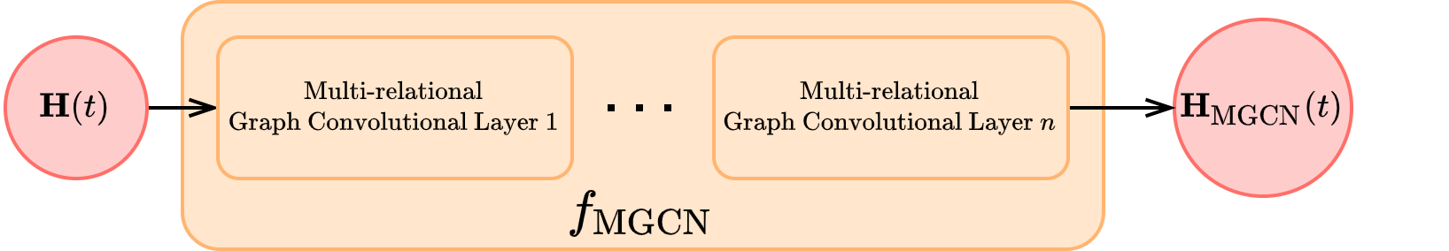
(a) $f_{\textrm{MGCN}}$

(b) $f_{\textrm{TANGO}}$

Figure 1: (a) The structure of $f_{\textrm{MGCN}}$: stacked multi-relational graph convolutional layers (the orange block). $\textbf{H}(t)$ denotes the hidden representations of entities and relations at time $t$. $\textbf{H}_{\textrm{MGCN}}(t)$ denotes the output of the stacked multi-relational graph convolutional layers. (b) The architecture of TANGO that parameterizes the derivatives of the hidden representations $\mathbf{H}(t)$. In addition to $f_{\textrm{MGCN}}$, a graph transition layer $f_{\textrm{trans}}$ is employed to model the edge formation and dissolution.

3.1 Neural ODE for Temporal KG

The temporal dynamics of a time-evolving multi-relational graph can be characterized by the following neural ordinary differential equation

$$\frac{d\textbf{H}(t)}{dt}= f_{\textrm{TANGO}}(\textbf{H}(t),\textbf{T}(t),\mathcal{G}(t),t)$$ (4)

$$= f_{\textrm{MGCN}}(\textbf{H}(t),\mathcal{G}(t),t)$$

$$+wf_{\textrm{trans}}(\textbf{H}(t),\textbf{T}(t),\mathcal{G}(t),t),$$

where $\textbf{H}\in R^{(|\mathcal{V}|+2|\mathcal{R}|)\times d}$ denotes the hidden representations of entities and relations. $f_{\textrm{TANGO}}$ represents the neural network that parameterizes the derivatives of the hidden representations. Besides, $f_{\textrm{MGCN}}$ denotes stacked multi-relational graph convolutional layers, $f_{\textrm{trans}}$ represents the graph transition layer, and $\mathcal{G}(t)$ denotes the snapshot of the temporal KG at time $t$. $\textbf{T}(t)$ contains the information on edge formation and dissolution since the last observation. $w$ is a hyperparameter controlling how much the model learns from edge formation and dissolution. We set $\textbf{H}(t=0)=\textrm{Emb}(\mathcal{V},\mathcal{R})$, where Emb($\mathcal{V},\mathcal{R}$) denotes the learnable initial embeddings of entities and relations on the temporal KG. Thus, given a time window $\Delta t$, the representation evolution performed by the neural ODE assumes the following form

$$\textbf{H}(t+\Delta t)-\textbf{H}(t)$$ (5)

$$=\int_{t}^{t+\Delta t}f_{\textrm{TANGO}}(\textbf{H}(\tau),\textbf{T}(\tau),\mathcal{G}(\tau),\tau)\,d\tau$$

$$=\int_{t}^{t+\Delta t}(f_{\textrm{MGCN}}(\textbf{H}(\tau),\mathcal{G}(\tau),\tau)$$

$$\quad\quad\quad\quad\ \ +wf_{\textrm{trans}}(\textbf{H}(\tau),\textbf{T}(\tau),\tau))d\tau.$$

In this way, we use the neural ODE to learn the dynamics of continuous-time temporal KGs.

3.2 Multi-Relational Graph Convolutional Layer

Inspired by Vashishth et al. (2019) and Yang et al. (2014), we use the entity-relation composition to model relational information. Specifically, we propose a multi-relational graph convolutional layer as follows. At time $t$, for every object entity $o\in\mathcal{V}$ with $\mathcal{N}(o)=\{(s,r)|(s,r,o,t)\in\mathcal{G}(t)\}$, its hidden representation evolves as

$$\widetilde{\textbf{h}}_{o}^{l+1}(t)=\frac{1}{|\mathcal{N}(o)|}\sum\limits_{(s,r)\in\mathcal{N}(o)}\textbf{W}^{l}(\textbf{h}_{s}^{l}(t)*\textbf{h}_{r}),$$ (6)

$$\textbf{h}_{o}^{l+1}(t)=\mathbf{h}_{o}^{l}(t)+\delta\sigma(\widetilde{\textbf{h}}_{o}^{l+1}(t)),$$

where $\mathbf{h}_{o}^{l+1}(t)$ denotes the hidden representation of the object $o$ at the $(l+1)^{th}$ layer, $\textbf{W}^{l}$ represents the weight matrix on the $l^{th}$ layer, $*$ denotes element-wise multiplication. $\mathbf{h}_{s}^{l}(t)$ means the hidden representation of the subject $s$ at the $l^{th}$ layer. $\mathbf{h}^{l=0}_{s}(t)=\mathbf{h}_{s}(t)$ is obtained by the ODE Solver that integrates Equation 4 until $t$. $\delta$ is a learnable weight. In this work, we assume that the relation representations do not evolve, and thus, $\mathbf{h}_{r}$ is time-invariant. We use $ReLU(\cdot)$ as the activation function $\sigma(\cdot)$. From the view of the whole tKG, we use $\mathbf{H}(t)$ to represent the hidden representations of all entities and relations on the tKG. Besides, we use $f_{\textrm{MGCN}}$ to denote the network consisting of multiple multi-relational graph convolutional layers (Equation 6).

3.3 Graph Transition Layer

To let the model focus on the graph’s transitions, we define a transition tensor for tKGs and use graph convolutions to capture the information of edge formation and dissolution. Given two graph snapshots $\mathcal{G}(t-\Delta t)$ and $\mathcal{G}(t)$ at time $t-\Delta t$ and $t$, respectively, the graph transition tensor $\mathbf{T}(t)$ is defined as

$$\textbf{T}(t)=\textbf{A}(t)-\textbf{A}(t-\Delta t),$$ (7)

where $\textbf{A}(t)\in\{0,1\}^{|\mathcal{V}|\times|\mathcal{R}|\times|\mathcal{V}|}$ is a three-way adjacency tensor whose entries are set such that

$$A_{sro}=\left\{\begin{aligned} &1,\textrm{if the triple $(s,r,o)$ exists at time $t$},\\ &0,\textrm{otherwise}.\end{aligned}\right.$$ (8)

Intuitively, $\textbf{T}(t)\in\{-1,0,1\}^{|\mathcal{V}|\times|\mathcal{R}|\times|\mathcal{V}|}$ contains the information of the edges’ formation and dissolution since the last observation $\mathcal{G}(t-\Delta t)$. Specifically, $T_{sro}(t)=-1$ means that the triple $(s,r,o)$ disappears at $t$, and $T_{sro}(t)=1$ means that the triplet $(s,r,o)$ is formatted at $t$. For all unchanged edges, their values in $\textbf{T}(t)$ are equal to $0$. Additionally, we use graph convolutions to extract the information provided by the graph transition tensor:

$$\widetilde{\textbf{h}}^{l+1}_{o,\textrm{trans}}(t)=\textbf{W}_{\textrm{trans}}(T_{sro}(t)(\textbf{h}^{l}_{s}(t)*\textbf{h}_{r}))$$ (9)

$$\textbf{h}^{l+1}_{o,\textrm{trans}}(t)=\sigma\left(\frac{1}{|\mathcal{N}_{T}(o)|}\sum\limits_{(s,r)\in\mathcal{N}_{T}(o)}\widetilde{\textbf{h}}^{l+1}_{o,\textrm{trans}}(t)\right)$$

Here, $\textbf{W}_{\textrm{trans}}$ is a trainable diagonal weight matrix and $\mathcal{N}_{T}(o)=\{(s,r)|T_{sro}(t)\neq 0)\}$. By employing this graph transition layer, we can better model the dynamics of temporal KGs. We use $f_{\textrm{trans}}$ to denote Equation 9. By combining the multi-relational graph convolutional layers $f_{\textrm{MGCN}}$ with the graph transition layer $f_{\textrm{trans}}$, we get our final network that parameterizes the derivatives of the hidden representations $\textbf{H}(t)$, as shown in Figure 1(b).

3.4 Learning and Inference

TANGO is an autoregressive model that forecasts the entity representation at time $t$ by utilizing the graph information before $t$. To answer a link forecasting query $(s,r,?,t)$, TANGO takes three steps. First, TANGO computes the hidden representations $\mathbf{H}(t)$ of entities and relations at the time $t$. Then TANGO uses a score function to compute the scores of all quadruples $\{(s,r,o,t)|o\in\mathcal{V}\}$ accompanied with candidate entities. Finally, TANGO chooses the object with the highest score as its prediction.

Representation inference

The representation inference procedure is done by an ODE Solver, which is $\mathbf{H}(t)=\textrm{ODESolver}(\textbf{H}(t-\Delta t),f_{\textrm{TANGO}},t-\Delta t,t,\Theta_{\textrm{TANGO}},\mathcal{G})$. Adaptive ODE solvers may incur massive time consumption in our work. To keep the training time tractable, we use fixed-grid ODE solvers coupled with the Interpolated Reverse Dynamic Method (IRDM) proposed by Daulbaev et al. (2020). IRDM uses Barycentric Lagrange interpolation Berrut and Trefethen (2004) on Chebyshev grid Tyrtyshnikov (2012) to approximate the solution of the hidden states in the reverse-mode of NODE. Thus, IRDM can lower the time cost in the backpropagation and maintain good learning accuracy. Additional information about representation inference is provided in Appendix A.

Score function

Given the entity and relation representations at the query time $t_{q}$, one can compute the scores of every triple at $t_{q}$. In our work, we take two popular knowledge graph embedding models, i.e., Distmult Yang et al. (2014) and TuckER Balazevic et al. (2019). Given triple $(s,r,o)$, its score is computed as shown in Table 1.

Table 1: Score Functions. $\textbf{h}_{s},\textbf{h}_{r},\textbf{h}_{o}$ denote the entity representations of the subject entity $s$, object entity $o$, and the representation of the relation $r$, respectively. $d$ denotes the hidden dimension of representations. $\mathcal{W}\in\mathbb{R}^{d\times d\times d}$ is the core tensor specified in Balazevic et al. (2019). As defined in Tucker (1964), $\times_{1},\times_{2},\times_{3}$ are three operators indicating the tensor product in three different modes.

Method	Score Function
Distmult Yang et al. (2014)	$<\textbf{h}_{s},\textbf{h}_{r},\textbf{h}_{o}>$	$\textbf{h}_{s},\textbf{h}_{r},\textbf{h}_{o}\in\mathbb{R}^{d}$
TuckER Balazevic et al. (2019)	$\mathcal{W}\times_{1}\textbf{h}_{s}\times_{2}\textbf{h}_{r}\times_{3}\textbf{h}_{o}$	$\textbf{h}_{s},\textbf{h}_{r},\textbf{h}_{o}\in\mathbb{R}^{d}$

Parameter Learning

For parameter learning, we employ the cross-entropy loss:

$$\mathcal{L}=\sum\limits_{(s,r,o,t)\in\mathcal{F}}-\textrm{log}(f(o|s,r,t,\mathcal{V})),$$ (10)

where $f(o|s,r,t,\mathcal{V})=\frac{\textrm{exp}(score(\mathbf{h}_{s}(t),\mathbf{h}_{r},\mathbf{h}_{o}(t)))}{\sum\limits_{e\in\mathcal{V}}\textrm{exp}(score(\mathbf{h}_{s}(t),\mathbf{h}_{r},\mathbf{h}_{e}(t)))}$. $e\in\mathcal{V}$ represents an object candidate, and $score(\cdot)$ is the score function. $\mathcal{F}$ summarizes valid quadruples of the given tKG.

4 Experiments

4.1 Experimental Setup

We evaluate our model by performing future link prediction on five tKG datasets. We compare TANGO’s performance with several existing methods and evaluate its potential with inductive link prediction and long horizontal link forecasting. Besides, an ablation study is conducted to show the effectiveness of our graph transition layer.

4.1.1 Datasets

We use five benchmark datasets to evaluate TANGO: 1) ICEWS14 Trivedi et al. (2017) 2) ICEWS18 Boschee et al. (2015) 3) ICEWS05-15 García-Durán et al. (2018) 4) YAGO Mahdisoltani et al. (2013) 5) WIKI Leblay and Chekol (2018). Integrated Crisis Early Warning System (ICEWS) Boschee et al. (2015) is a dataset consisting of timestamped political events, e.g., (Barack Obama, visit, India, 2015-01-25). Specifically, ICEWS14 contains events occurring in 2014, while ICEWS18 contains events from January 1, 2018, to October 31, 2018. ICEWS05-15 is a long-term dataset that contains the events between 2005 and 2015. WIKI and YAGO are two subsets extracted from Wikipedia and YAGO3 Mahdisoltani et al. (2013), respectively. The details of each dataset and the dataset split strategy are provided in Appendix D.

4.1.2 Evaluation Metrics

We use two metrics to evaluate the model performance on extrapolated link prediction, namely Mean Reciprocal Rank (MRR) and Hits@1/3/10. MRR is the mean of the reciprocal values of the actual missing entities’ ranks averaged by all the queries, while Hits@1/3/10 denotes the proportion of the actual missing entities ranked within the top 1/3/10. The filtering settings have been implemented differently by various authors. We report results based on two common implementations: $i)$ time-aware (Han et al., 2021) and $ii)$ time-unaware filtering (Jin et al., 2019). We provide a detailed evaluation protocol in Appendix B.

4.1.3 Baseline Methods

We compare our model performance with nine baselines. We take three static KG models as the static baselines, including Distmult Yang et al. (2014), TuckER Balazevic et al. (2019), and COMPGCN Vashishth et al. (2019). For tKG baselines, we report the performance of TTransE (Leblay and Chekol, 2018), TA-Distmult García-Durán et al. (2018), CyGNet (Zhu et al., 2020), DE-SimplE (Goel et al., 2020), TNTComplEx (Lacroix et al., 2020), and RE-Net Jin et al. (2019). We provide implementation details of baselines and TANGO in Appendix C.

4.2 Experimental Results

4.2.1 Time-aware filtered Results

Datasets	ICEWS05-15 - aware filtered				ICEWS14 - aware filtered				ICEWS18 - aware filtered				WIKI - aware filtered				YAGO - aware filtered
Model	MRR	Hits@1	Hits@3	Hits@10	MRR	Hits@1	Hits@3	Hits@10	MRR	Hits@1	Hits@3	Hits@10	MRR	Hits@1	Hits@3	Hits@10	MRR	Hits@1	Hits@3	Hits@10
Distmult	24.75	16.10	27.67	42.42	14.49	8.15	15.31	27.66	16.69	9.68	18.12	31.21	49.66	46.17	52.81	54.13	54.84	47.39	59.81	68.52
TuckER	27.13	17.01	29.93	47.81	18.96	11.23	20.77	33.94	20.68	12.58	22.60	37.27	50.01	46.12	53.60	54.86	54.86	47.42	59.63	68.96
CompGCN	29.68	20.72	32.51	47.87	17.81	10.12	19.49	33.11	20.56	12.01	22.96	38.15	49.88	45.78	52.91	55.58	54.35	46.72	59.26	68.29
TTransE	21.24	4.98	31.48	49.88	9.67	1.25	12.29	28.37	8.08	1.84	8.25	21.29	29.27	21.67	34.43	42.39	31.19	18.12	40.91	51.21
TA-DistMult	24.39	14.77	27.80	44.22	10.34	4.72	10.54	21.48	11.38	5.58	12.04	22.82	44.53	39.92	48.73	51.71	54.92	48.15	59.61	66.71
CyGNet	35.79	26.09	40.18	54.48	22.83	14.28	25.36	39.97	24.93	15.90	28.28	42.61	33.89	29.06	36.10	41.86	52.07	45.36	56.12	63.77
DE-SimplE	35.57	26.33	39.41	53.97	21.58	13.77	23.68	37.15	19.30	11.53	21.86	34.80	45.43	42.6	47.71	49.55	54.91	51.64	57.30	60.17
TNTComplEx	35.88	26.92	39.55	53.43	23.81	15.58	26.27	40.12	21.23	13.28	24.02	36.91	45.03	40.04	49.31	52.03	57.98	52.92	61.33	66.69
RE-Net	40.23	30.30	44.83	59.59	25.66	16.69	28.35	43.62	27.90	18.45	31.37	46.37	49.66	46.88	51.19	53.48	58.02	53.06	61.08	66.29
-TuckER	42.86	32.72	48.14	62.34	26.25	17.30	29.07	44.18	28.97	19.51	32.61	47.51	51.60	49.61	52.45	54.87	62.50	58.77	64.73	68.63
	$\pm$ 0.2	$\pm$ 0.3	$\pm$ 0.2	$\pm$ 0.2	$\pm$ 0.1	$\pm$ 0.1	$\pm$ 0.1	$\pm$ 0.1	$\pm$ 0.2	$\pm$ 0.1	$\pm$ 0.2	$\pm$ 0.3	$\pm$ 0.3	$\pm$ 0.2	$\pm$ 0.3	$\pm$ 0.3	$\pm$ 0.5	$\pm$ 0.2	$\pm$ 0.1	$\pm$ 0.4
-Distmult	40.71	31.23	45.33	58.95	24.70	16.36	27.26	41.35	27.56	18.68	30.86	44.94	53.04	51.52	53.84	55.46	63.34	60.04	65.19	68.79
	$\pm$ 0.3	$\pm$ 0.4	$\pm$ 0.1	$\pm$ 0.5	$\pm$ 0.1	$\pm$ 0.1	$\pm$ 0.1	$\pm$ 0.1	$\pm$ 0.2	$\pm$ 0.2	$\pm$ 0.2	$\pm$ 0.3	$\pm$ 0.3	$\pm$ 0.4	$\pm$ 0.2	$\pm$ 0.1	$\pm$ 0.4	$\pm$ 0.4	$\pm$ 0.1	$\pm$ 0.2

Table 2: Extrapolated link prediction results on five datasets. Evaluation metrics are time-aware filtered MRR (%) and Hits@1/3/10 (%). denotes TANGO. The best results are marked in bold.

We run TANGO five times and report the averaged results. The time-aware filtered results are presented in Table 2, where denotes TANGO. As explained in Appendix B, we take the time-aware filtered setting as the fairest evaluation setting. Results demonstrate that TANGO outperforms all the static baselines on every dataset. This implies the importance of utilizing temporal information in tKG datasets. The comparison between Distmult and TANGO-Distmult shows the superiority of our NODE-based encoder, which can also be observed by the comparison between TuckER and TANGO-TuckER. Additionally, TANGO achieves much better results than COMPGCN, indicating our method’s strength in incorporating temporal features into tKG representation learning.

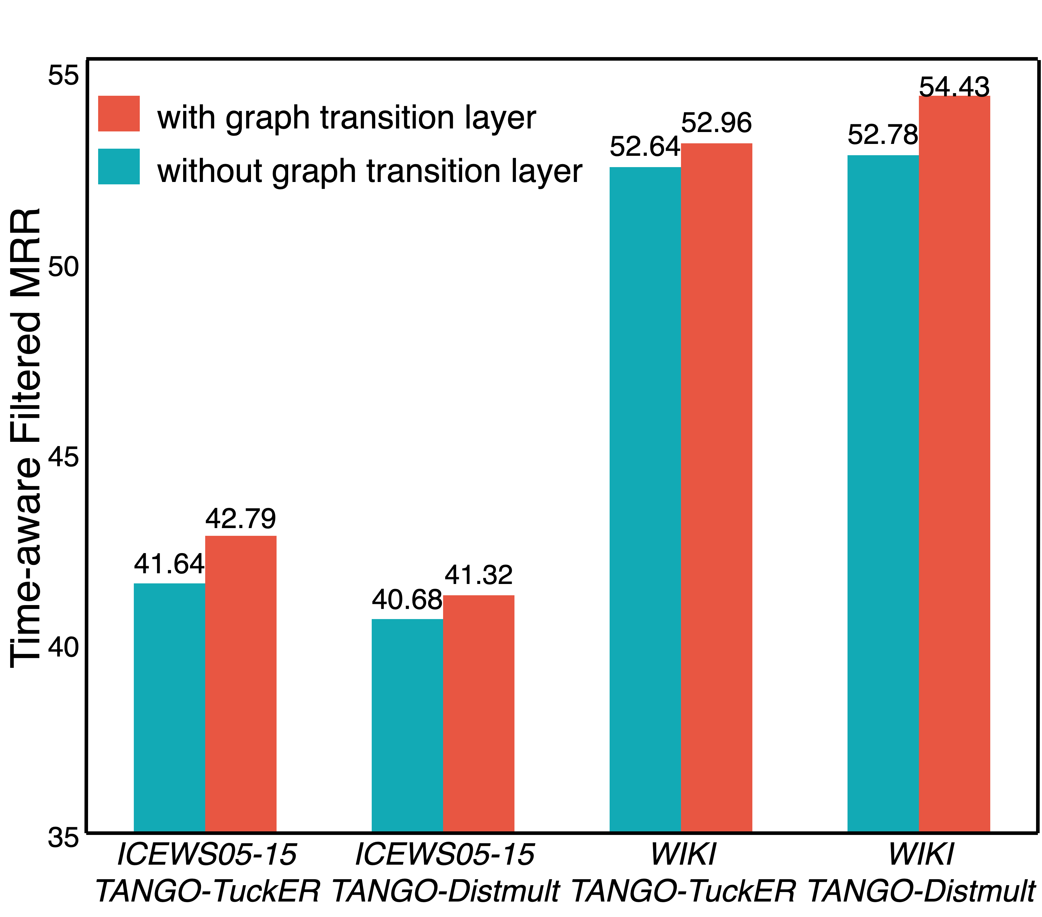
Figure 2: Time-aware filtered MRR of TANGO with or without the graph transition layer on subsets of ICEWS05-15 and WIKI. We split the graph snapshots into two groups, where the transition tensor’s norm $||\mathbf{T}(t)||_{L1}$ of each graph snapshot in the first group is larger than that of all graph snapshots in the second group. Since the graph transition layer is tailored to graph changes, we show the results of the first group here. The corresponding result of the ablation study on the whole test sets are presented in Figure 8 in the appendix.

Similarly, TANGO outperforms all the tKG baselines as well. Unlike TTransE and TA-Distmult, RE-Net uses a recurrent neural encoder to capture temporal information, which shows great success on model performance and is the strongest baseline. Our model TANGO implements a NODE-based encoder in the recurrent style to capture temporal dependencies. It consistently outperforms RE-Net on all datasets because TANGO explicitly encodes time information into hidden representations while RE-Net only considers the temporal order between events. Additionally, we provide the raw and time-unaware filtered results in Table 5 and 4 in the appendix.

4.2.2 Ablation Study

To evaluate the effectiveness of our graph transition layer, we conduct an ablation study on two datasets, i.e., ICEWS05-15 and WIKI. We choose these two datasets as the representative of two types of tKG datasets. ICEWS05-15 contains events that last shortly and happen multiple times, i.e., Obama visited Japan. In contrast, the events in the WIKI datasets last much longer and do not occur periodically, i.e., Eliran Danin played for Beitar Jerusalem FC between 2003 and 2010. The improvement of the time-aware filtered MRR brought by the graph transition layer is illustrated in Figure 2, showing that the graph transition layer can effectively boost the model performance by incorporating the edge formation and dissolution information.

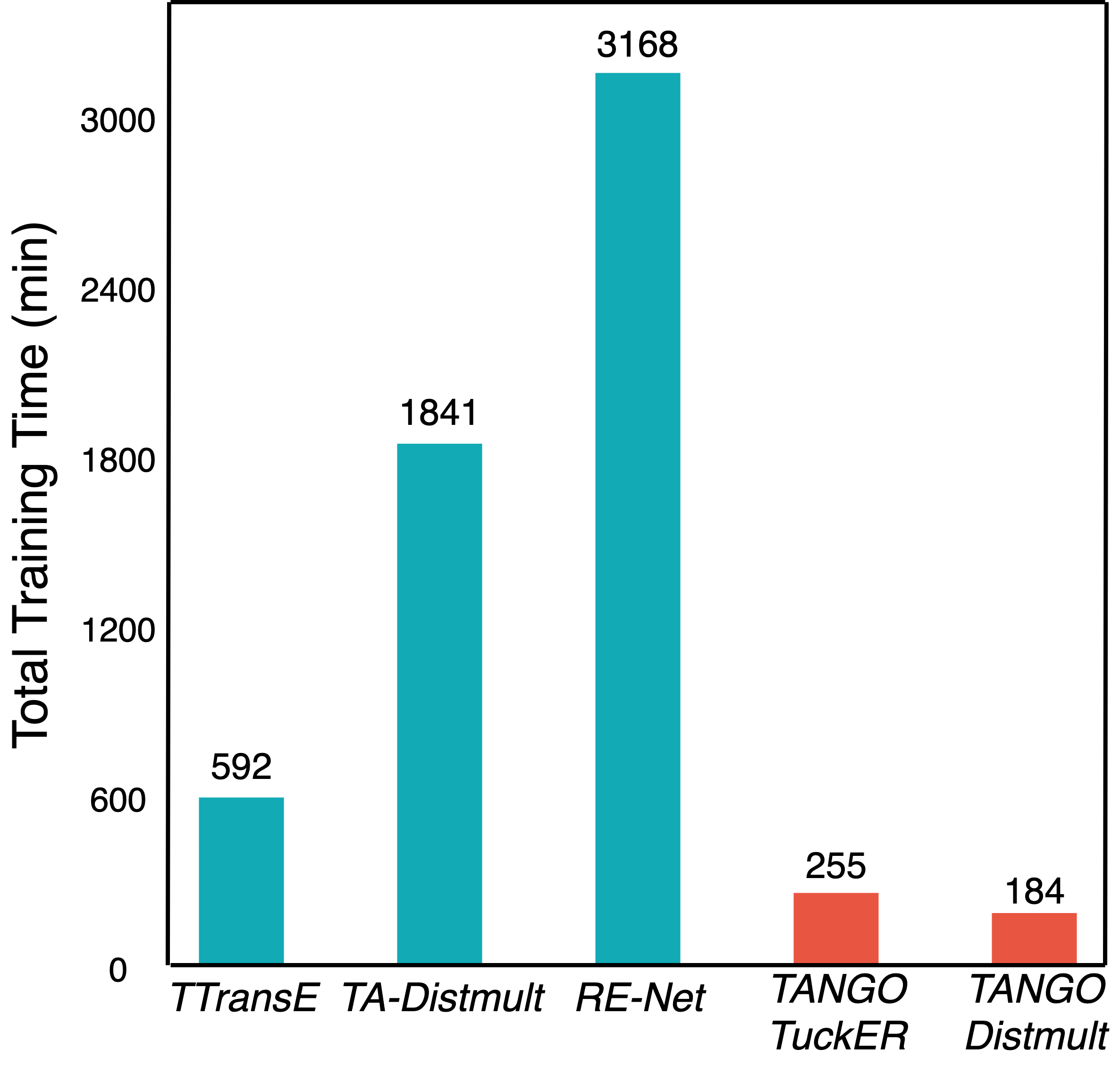
Figure 3: Time cost comparison on ICEWS05-15. Columns marked as orange denote the time consumed by our model.

4.2.3 Time Cost Analysis

Keeping training time short while achieving a strong performance is significant in model evaluation. We report in Figure 3 the total training time of our model and the baselines on ICEWS05-15. We see that static KG reasoning methods generally require less training time than temporal methods. Though the total training time for TTransE is short, its performance is low, as reported in the former sections. TA-Distmult consumes more time than our model and is also beaten by TANGO in performance. RE-Net is the strongest baseline in performance; however, it requires almost ten times as much as the total training time of TANGO. TANGO ensures a short training time while maintaining the state-of-the-art performance for future link prediction, which shows its superiority.

Datasets	ICEWS05-15 - raw				ICEWS05-15 - aware filtered				ICEWS05-15 - unaware filtered
Model	MRR	Hits@1	Hits@3	Hits@10	MRR	Hits@1	Hits@3	Hits@10	MRR	Hits@1	Hits@3	Hits@10
RE-Net	4.96	2.20	5.39	10.12	5.02	2.29	5.49	10.12	5.50	2.95	5.93	10.26
-TuckER w.o.trans	5.13	2.58	5.67	9.91	5.18	2.64	5.70	9.94	5.98	3.34	6.71	10.67
-Distmult w.o.trans	3.72	2.05	3.80	6.76	3.76	2.09	3.82	6.77	4.09	2.46	4.17	6.99
-TuckER	5.74	3.07	6.48	10.74	5.81	3.16	6.52	10.78	6.75	4.11	7.60	11.54
-Distmult	5.00	2.70	5.67	9.16	5.05	2.78	5.69	9.17	5.69	3.45	6.27	9.69

Table 3: Inductive future link prediction results on ICEWS05-15. Evaluation metrics are raw, time-aware filtered, and time-unaware filtered MRR (%), Hits@1/3/10 (%). w.o.trans means without the graph transition layer. The best results are marked in bold.

4.3 New Evaluation Tasks

4.3.1 Long Horizontal Link Forecasting

Given a sequence of observed graph snapshots until time $t$, the future link prediction task infers the quadruples happening at $t+\Delta t$. $\Delta t$ is usually small, i.e., one day, in standard settings (Trivedi et al., 2017; Jin et al., 2019; Zhu et al., 2020). However, in some scenarios, the graph information right before the query time is likely missing. This arouses the interest in evaluating the temporal KG models by predicting the links in the farther future. In other words, given the same input, the model should predict the links happening at $t+\Delta T$, where $\Delta T>>\Delta t$. Based on this idea, we define a new evaluation task, e.g., long horizontal link forecasting.

Figure 4: Long horizontal link forecasting: time-aware filtered MRR (%) on ICEWS05-15 with regard to different $\Delta t$.

To perform long horizontal link forecasting, we adjust the integral length according to how far the future we want to predict. As described in Figure 5, the integration length between the neighboring timestamps is short for the first $k$ steps, e.g., integration from $(t-t_{k})$ to $(t-t_{k}+\Delta t)$. However, for the last step, e.g., integration from $t$ to $t+\Delta T$, the integration length becomes significantly large according to how far the future we want to predict. The larger $\Delta T$ is, the longer the length is for the last integration step.

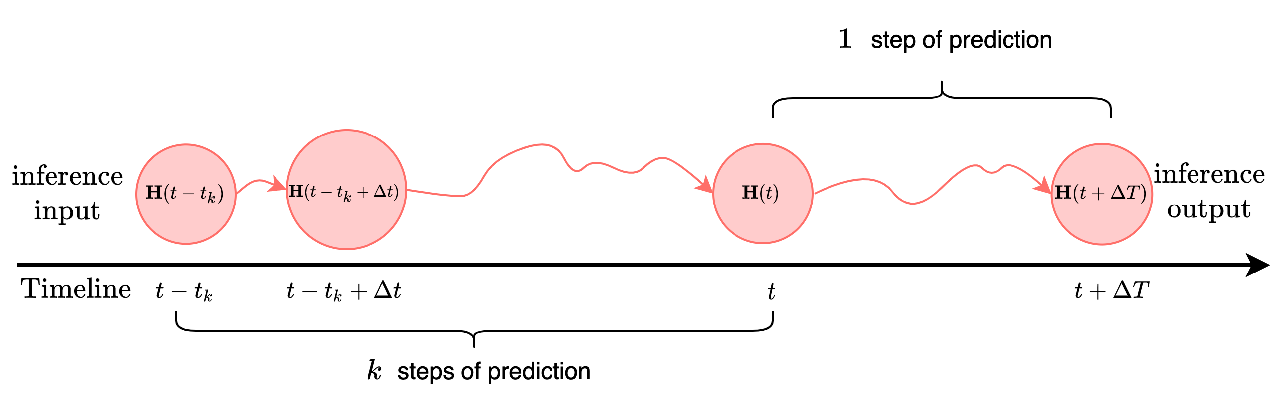
Figure 5: Graphical illustration of long horizontal link forecasting. Given a sequence of graph snapshots $\mathbb{G}=\{\mathcal{G}(t-t_{k}),...,\mathcal{G}(t)\}$, whose length is $k$, test quadruples at $t+\Delta T$ are to be predicted.

We report the results corresponding to different $\Delta T$ on ICEWS05-15 and compare our model with the strongest baseline RE-Net. In Figure 4, we observe that our model outperforms RE-Net in long horizontal link forecasting. The gap between the performances of the two models diminishes as $\Delta T$ increases. This trend can be explained in the following way. Our model employs an ODE solver to integrate the graph’s hidden states over time. Since TANGO takes the time information into account and integrates the ODE in the continuous-time domain, its performance is better than RE-Net, which is a discrete-time model. However, TANGO assumes that the dynamics it learned at $t$ also holds at $t+\Delta T$. This assumption holds when $\Delta T$ is small. As $\Delta T$ increases, the underlying dynamics at $t+\Delta T$ would be different from the dynamics at $t$. Thus, the TANGO’s performance degrades accordingly, and the advancement compared to RE-Net also vanishes.

4.3.2 Inductive Link Prediction

New graph nodes might emerge as time evolves in many real-world applications, i.e., new users and items. Thus, a good model requires a strong generalization power to deal with unseen nodes. We propose a new task, e.g., inductive link prediction, to validate the model potential in predicting the links regarding unseen entities at a future time. A test quadruple is selected for the inductive prediction if either its subject or object or both haven’t been observed in the training set. For example, in the test set of ICEWS05-15, we have a quadruple (Raheel Sharif, express intent to meet or negotiate, Chaudhry Nisar Ali Khan, 2014-12-29). The entity Raheel Sharif does not appear in the training set, indicating that the aforementioned quadruple contains an entity that the model does not observe in the training set. We call the evaluation of this kind of test quadruples the inductive link prediction analysis.

We perform the future link prediction on these inductive link prediction quadruples, and the results are shown in Table 3. We compare our model with the strongest baseline RE-Net on ICEWS05-15. We also report the results achieved by TANGO without the graph transition layer to show the performance boost brought by it. As shown in Table 3, TANGO-TuckER achieves the best results across all metrics. Both TANGO-TuckER and TANGO-Distmult can beat RE-Net, showing the strength of our model in inductive link prediction. The results achieved by the TANGO models are much better than their variants without the graph transition layers, which proves that the proposed graph transition layer plays an essential role in inductive link prediction.

5 Conclusions

We propose a novel representation method, TANGO, for forecasting future links on temporal knowledge graphs (tKGs). We propose a multi-relational graph convolutional layer to capture structural dependencies on tKGs and learn continuous dynamic representations using graph neural ordinary differential equations. Especially, our model is the first one to show that the neural ODE can be extended to modeling dynamic multi-relational graphs. Besides, we couple our model with the graph transition layer to explicitly capture the information provided by the edge formation and deletion. According to the experimental results, TANGO achieves state-of-the-art performance on five benchmark datasets for tKGs. We also propose two new tasks to evaluate the potential of link forecasting models, namely inductive link prediction and long horizontal link forecasting. TANGO performs well in both tasks and shows its great potential.

Appendix

Datasets	ICEWS05-15 - raw				ICEWS14 - raw				ICEWS18 - raw				WIKI - raw				YAGO - raw
Model	MRR	Hits@1	Hits@3	Hits@10	MRR	Hits@1	Hits@3	Hits@10	MRR	HITS@1	HITS@3	HITS@10	MRR	Hits@1	Hits@3	Hits@10	MRR	Hits@1	Hits@3	Hits@10
Distmult	24.55	15.85	27.53	42.17	14.00	7.72	14.65	27.16	16.30	9.25	17.67	30.93	42.08	34.29	48.69	53.25	47.66	36.59	55.89	67.45
TuckER	26.95	16.81	29.69	47.61	18.39	10.69	20.01	33.42	20.20	12.08	21.99	36.91	42.50	34.41	49.41	53.90	47.48	36.20	55.55	68.07
COMPGCN	29.41	20.41	32.17	47.65	17.13	9.36	18.84	32.54	19.98	11.45	22.25	37.73	42.33	34.02	48.65	54.63	47.08	65.36	66.90	68.81
TTransE	20.89	4.88	3.11	49.66	9.21	1.12	11.19	27.46	7.92	1.75	8.00	21.02	19.53	12.34	23.11	32.47	26.18	12.36	36.16	48.00
TA-DistMult	24.03	14.37	27.36	44.04	9.92	4.39	9.99	20.90	11.05	5.24	11.72	22.55	27.33	19.94	32.05	39.42	45.54	36.54	51.08	62.15
RE-Net	39.31	28.88	44.40	59.38	23.84	14.60	26.48	42.58	26.62	16.91	30.26	45.82	31.10	25.31	34.13	41.33	46.28	37.52	51.77	61.55
-TuckER	41.82	31.10	47.55	62.19	24.36	15.12	27.15	43.07	27.59	17.77	31.40	46.92	31.99	25.74	35.00	42.61	49.31	40.78	55.12	63.73
-Distmult	40.23	30.53	44.95	59.05	22.87	14.22	25.43	40.32	26.21	16.92	29.77	44.41	32.53	26.33	35.75	43.17	49.49	40.90	55.42	63.74

Table 4: Future link prediction results on benchmark datasets. Evaluation metrics are raw MRR (%) and Hits@1/3/10 (%). denotes TANGO. The best results are marked in bold.

Datasets	ICEWS05-15 - unaware filtered				ICEWS14 - unaware filtered				ICEWS18 - unaware filtered				WIKI - unaware filtered				YAGO - unaware filtered
Model	MRR	Hits@1	Hits@3	Hits@10	MRR	Hits@1	Hits@3	Hits@10	MRR	Hits@1	Hits@3	Hits@10	MRR	Hits@1	Hits@3	Hits@10	MRR	Hits@1	Hits@3	Hits@10
Distmult	48.77	43.85	51.22	57.99	33.88	27.86	36.16	45.14	40.28	36.04	41.78	48.36	53.22	52.61	53.41	54.20	67.55	66.76	67.49	69.11
TuckER	58.69	54.74	59.82	66.57	46.51	41.11	49.45	57.34	44.50	38.33	46.11	53.71	53.97	52.70	54.15	54.94	67.40	66.22	67.62	69.84
COMPGCN	49.60	43.13	52.85	61.59	38.15	31.04	41.00	51.44	35.68	27.87	39.38	49.94	53.54	52.29	53.61	55.76	66.66	65.36	66.90	68.81
TTransE	28.81	5.83	48.67	60.38	15.95	1.57	25.98	42.67	10.52	3.01	11.98	26.16	31.94	24.82	36.91	43.55	33.73	20.99	43.51	52.61
TA-DistMult	38.54	29.94	42.92	54.81	18.74	11.97	20.32	31.95	16.27	10.22	17.39	27.91	50.18	48.65	51.41	52.37	66.06	64.36	66.78	68.74
RE-Net	57.66	51.86	60.40	68.60	45.24	37.82	48.53	58.92	43.02	36.26	45.61	56.03	52.27	50.92	52.73	53.57	64.68	62.94	65.11	67.82
-TuckER	59.93	54.99	62.65	69.64	46.42	38.94	50.25	59.80	44.56	37.87	47.46	57.06	53.28	52.21	53.61	54.84	67.21	65.56	67.59	70.04
-Distmult	58.89	54.42	60.76	67.47	46.68	41.20	48.64	57.05	44.00	38.64	45.78	54.27	54.05	51.52	53.84	55.46	68.34	67.05	68.39	70.70

Table 5: Future link prediction results on benchmark datasets. Evaluation metrics are time-unaware filtered MRR (%) and Hits@1/3/10 (%). denotes TANGO. The best results are marked in bold.

Datasets	ICEWS05-15 - aware filtered				ICEWS18 - aware filtered				WIKI - aware filtered				YAGO - aware filtered
Model	MRR	Hits@1	Hits@3	Hits@10	MRR	Hits@1	Hits@3	Hits@10	MRR	Hits@1	Hits@3	Hits@10	MRR	Hits@1	Hits@3	Hits@10
-TuckER	44.57	34.40	49.94	63.95	30.68	20.75	34.61	50.43	62.29	59.54	63.92	66.63	69.29	64.33	72.40	77.63
-Distmult	43.33	33.46	48.45	62.05	29.62	20.18	33.35	48.36	63.93	62.14	64.74	67.06	70.79	66.15	74.04	78.18

Table 6: Validation results on benchmark datasets regarding our model. Evaluation metrics are time-aware filtered MRR (%) and Hits@1/3/10 (%). denotes TANGO. The best results are marked in bold. ICEWS14 has no validation set.

Appendix A Representation Inference

Assume we want to forecast a link at $t$. We take the graph histories between the timestamp $(t-t_{k})$ and the timestamp $t$ into account, where $t_{k}$ indicates the length of history. To infer the hidden representations $\mathbf{H}(t)$, we first use the initial embeddings $\textrm{Emb}(\mathcal{V},\mathcal{R})$ to approximate the hidden representations $\textbf{H}(t-t_{k})$. Then we take $\textbf{H}(t-t_{k})$ as the NODE input at the timestamp $(t-t_{k})$, and integrate it with an ODE solver $\textrm{ODESolver}(\textbf{H}(t-t_{k}),f_{\textrm{TANGO}},t-t_{k},t,\Theta_{\textrm{TANGO}},\mathcal{G})$ over time. As the hidden state evolves with time, it learns from different graph observations taken at different time. The whole process is described in Figure 6 and Algorithm 1. In Figure 6, set_graph and set_transition stand for two functions used to feed graph snapshots and the transition tensors into the neural network $f_{\textrm{TANGO}}$. They are called at every observation time before integration.

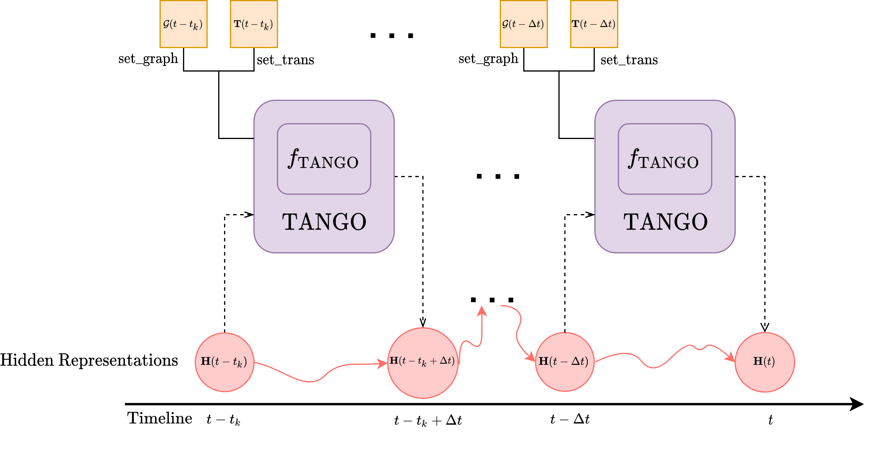
Figure 6: Illustration of the inference procedure. The shaded purple area represents the whole architecture of TANGO. It is a Neural ODE equipped with a GNN-based module $f_{\textrm{TANGO}}$. Dashed arrows denote the input and the output path of the graph’s hidden state. Red solid arrows indicate the continuous hidden state flows learned by TANGO. Black solid lines represent that TANGO calls the function set_graph and set_trans. The corresponding graph snapshots $\mathcal{G}$ and transition tensors T are input into $f_{\textrm{TANGO}}$ for learning temporal dynamics.

Appendix B Evaluation Metrics

We report the results in three settings, namely raw, time-unaware filtered, and time-aware filtered. For time-unaware filtered results, we follow the filtered evaluation constraint applied in Bordes et al. (2013); Jin et al. (2019), where we remove from the list of corrupted triplets all the triplets that appear either in the training, validation, or test set except the triplet of interest. Time-unaware filtering setting is inappropriate for temporal KG reasoning, while the time-aware filtering setting provides fairer results. For time-aware filtered results, we follow the setting proposed by Han et al. (2021) by only removing from the list of corrupted triplets all the triplets that appear at the query time $t_{q}$. The following example illustrates the reason why the time-aware filtered results are fairer than the time-unaware filtered results. Assume we have a test quadruple of interest (Xi Jinping, make a visit, New Zealand, 2014-11-26) in the test set, and we derive an object prediction query (Xi Jinping, make a visit, $?$, 2014-11-26) from this quadruple where the query time is 2014-11-26. Additionally, we have another quadruple (Xi Jinping, make a visit, South Korea, 2014-07-05) in the test set. According to the time-unaware filtering setting Bordes et al. (2013), (Xi Jinping, make a visit, South Korea) will be filtered out since it appears in the test set. However, it is unreasonable because (Xi Jinping, make a visit, South Korea) is not valid at 2014-11-26. Therefore, we use the time-aware filtered setting, which, in our example, will only filter the triplets (Xi Jinping, make a visit, $o$) appearing at 2014-11-26. Here, $o$ denotes all the objects from triplets accompanied with Xi Jinping, Make a visit, and the date 2014-11-26.

Appendix C Implementation Details

We train TANGO with the following settings. We tune the model across a range of hyperparameters as shown in Table 7. We do 432 trials, and each trial runs 20 epochs. We select the best-performing configuration according to filtered MRR on validation data. The best configuration will be further trained until its convergence. We run the selected configuration five times and obtain an averaged results. Specifically, we use a fixed-grid ODE solver, fourth-order Runge-Kutta, as the ODE solver, and implement the interpolated reverse dynamic method Daulbaev et al. (2020) with 3 Chebyshev nodes to keep training time tractable while maintaining high precision. To improve the ODE solver’s precision, we re-scale the time range of each dataset from 0 to 0.01 (or 0.1). This step restricts the length of ODE integration, preventing the high error induced by ODE solvers. For each query, we set the time range of the input history $t_{k}$ to 4 days for the ICEWS datasets. For WIKI and YAGO, we set $t_{k}$ to 4 years. Besides, we choose different values for the transition coefficient $w$ for different datasets. Our model is implemented with PyTorch Paszke et al. (2019), and the experiments are run on GeForce RTX 2080 Ti. A detailed report of the best configuration is provided in Table 8.

We implement Distmult in PyTorch and use the binary cross-entropy loss for learning parameters. We use the official implementation of  TuckER, COMPGCN, and RE-Net. For a fair comparison, we choose to use the variant of RE-Net with ground truth history during multi-step inference, and thus the model knows all the interactions before the time for testing. Besides, we set the history length of RE-Net to 10 and use the max-pooling in the global model. Additionally, we use the implementation of TTransE and TA-Distmult provided in Jin et al. (2019). For TA-Distmult, the vocabulary of temporal tokens consists of year, month, and day for all the datasets. We use the released code to implement DE-SimplE, TNTComplEx, and CyGNet. All the baselines are trained with Adam Optimizer Kingma and Ba (2017), and the batch size is set to 512.

Table 7: Search space of hyperparameters. $w$ represents the weight controlling how much the model learns from edge formation and dissolution. Scale represents the time range re-scaling parameter as introduced in C.

Hyperparameter	Search space
Embedding size	{200, 300}
# MGCN layer	{2, 3}
Decoder	{TuckER, Distmult}
Scale	{0.001, 0.01, 0.1}
$w$	{0.01, 0.1, 1}
Dropout	{0.3, 0.5}
History length	{4, 6, 10}

Table 8: Best hyperparameter settings on each dataset.

Datasets	ICEWS14	ICEWS18	ICEWS05-15	WIKI	YAGO
Hyperparameter
Embedding size	200	200	200	200	300
# MGCN layer	2	2	2	2	3
Decoder	TuckER	TuckER	TuckER	Distmult	Distmult
Scale	0.01	0.1	0.1	0.1	0.1
$w$	0.01	1	0.01	1	1
Dropout	0.3	0.3	0.3	0.3	0.3
History length	4	4	4	4	4

Appendix D Datasets

Table 9 We follow the data preprocessing method and the dataset split strategy proposed in Jin et al. (2019). Specifically, we split each dataset except ICEWS14 in chronological order into three parts, e.g., $80\%/10\%/10\%$ (training/validation/test). For ICEWS14, we split it into the training set and testing set with $50\%/50\%$ since ICEWS14 is not provided with a validation set. As explained in Jin et al. (2019), the difference between the first type (ICEWS) and the second type (WIKI and YAGO) of tKG datasets is that the first type datasets are events that often last shortly and happen multiple times, i.e., Obama visited Japan four times. In contrast, the events in the second type datasets last much longer and do not occur periodically, i.e., Eliran Danin played for Beitar Jerusalem FC between 2003 and 2010.

Dataset	$N_{\textrm{train}}$	$N_{\textrm{valid}}$	$N_{\textrm{test}}$	$|\mathcal{V}|$	$|\mathcal{R}|$	$N_{\textrm{obs}}$
ICEWS14 Trivedi et al. (2017)	$323,895$	$-$	$341,409$	$12,498$	$260$	$365$
ICEWS18 Boschee et al. (2015)	$373,018$	$45,995$	$49,545$	$23,033$	$256$	$304$
ICEWS05-15 García-Durán et al. (2018)	$369,104$	$46,188$	$46,037$	$10,488$	$251$	$4,017$
WIKI Leblay and Chekol (2018)	$539,286$	$67,538$	$63,110$	$12,554$	$24$	$232$
YAGO Mahdisoltani et al. (2013)	$161,540$	$19,523$	$20,026$	$10,623$	$10$	$189$

Table 9: Dataset statistics. $N_{\textrm{train}}$, $N_{\textrm{valid}}$, $N_{\textrm{test}}$ represent the number of quadruples in the training set, validation set, and test set, respectively. $N_{\textrm{obs}}$ denotes the number of observations, where we take a snapshot of the tKG at each observation.

Appendix E Impact of Past History Length

As mentioned in A, TANGO utilizes the previous histories between $(t-t_{k})$ and $t$ to forecast a link at $t$, where $t_{k}$ is a hyperparameter. Figure 7 shows the performance with various lengths of past histories along with the corresponding training time. When TANGO uses longer histories, MRR is getting higher. However, a long history requires more forwarding inferences. The choice of history length is a trade-off between the performance and computational cost. We observe that the gain of MRR compared to the training time is not significant when the length of history is four and over. Thus, the history length of four is chosen in our experiments.

Figure 7: Time-aware filtered MRR (%) and Training Time (seconds) on ICEWS05-15 corresponding to different history length (days).

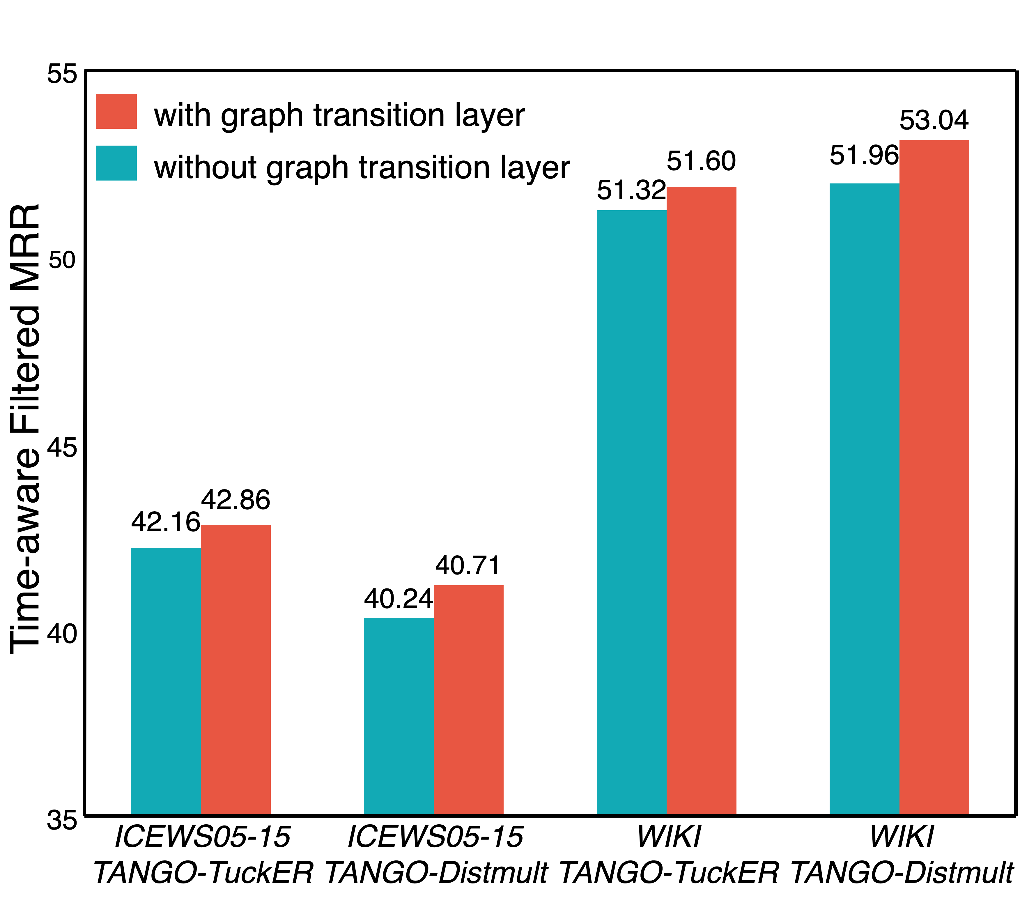
Figure 8: Time-aware filtered MRR of TANGO with or without the graph transition layer on the whole test sets of ICEWS05-15 and WIKI.

Datasets	ICEWS05-15 continuous - aware filtered				ICEWS05-15 - aware filtered
Model	MRR	Hits@1	Hits@3	Hits@10	MRR	Hits@1	Hits@3	Hits@10
TTransE	20.55	5.36	29.80	47.54	21.24	4.98	31.48	49.88
CyGNet	34.13	25.06	37.85	51.94	35.79	26.09	40.18	54.48
DE-SimplE	33.56	24.79	37.32	50.63	35.57	26.33	39.41	53.97
TNTComplEx	33.96	24.93	37.86	51.30	35.88	26.92	39.55	53.43
-TuckER	37.69	28.01	45.00	59.05	42.86	32.72	48.14	62.34
-Distmult	36.91	26.91	40.28	54.34	40.71	31.23	45.33	58.95

Table 10: Future link prediction results on ICEWS05-15 continuous dataset. Evaluation metrics are time-aware filtered MRR (%) and Hits@1/3/10 (%). denotes TANGO. The best results are marked in bold.

Dataset	$N_{\textrm{train}}$	$N_{\textrm{valid}}$	$N_{\textrm{test}}$	$|\mathcal{V}|$	$|\mathcal{R}|$	$N_{\textrm{obs}}$
ICEWS05-15 continuous	$149,001$	$17,962$	$17,902$	$10,488$	$251$	$1,589$

Table 11: Dataset statistics. $N_{\textrm{train}}$, $N_{\textrm{valid}}$, $N_{\textrm{test}}$ represent the number of quadruples in the training set, validation set, and test set, respectively. $N_{\textrm{obs}}$ denotes the number of observations, where we take a snapshot of the tKG at each observation.

Appendix F Analysis on Temporal KGs with Irregular Time Intervals

Most existing tKG reasoning models cannot properly deal with temporal KGs with irregular time intervals, while TANGO model them much better due to the nature of Neural ODE. We verify this via experiments on a new dataset. We call it ICEWS05-15_continuous. We sample the timestamps in ICEWS05-15 and keep the time intervals between each two of them in a range from 1 to 4. We only keep the temporal KG snapshots at the sampled time and extract a new subset. ICEWS05-15_continuous fits the setting when observations are taken non-periodically in continuous time. The dataset statistics of ICEWS05-15_continuous is reported in Table 11. We train our model and baseline methods on it and evaluate them with time-aware filtered MRR. As shown in Table 10, we validate that TANGO performs well on temporal KGs with irregular time intervals.

Appendix G Average runtime for each approach

Table 12 show the average runtime for each model.

Table 12: Average training time (second) until convergence

Datasets	ICEWS14	ICEWS18	ICEWS05-15	WIKI	YAGO
Model	Runtime	Runtime	Runtime	Runtime	Runtime
Distmult	743	1,365	401	2,245	3,310
TuckER	730	3,147	1,626	5,093	2,795
COMPGCN	9,226	6,432	1,607	5,810	2,233
TTransE	15,840	23,894	35,520	19,337	5,395
TA-Distmult	6,232	112,188	110,460	83,999	27,833
RE-Net	33,313	46,068	190,076	42,983	27,489
-TuckER	5,796	3,786	15,301	9,218	2,355
-Distmult	3,593	2,883	11,085	15,086	5,106

References

- Balazevic et al. (2019) Ivana Balazevic, Carl Allen, and Timothy Hospedales. 2019. TuckER: Tensor factorization for knowledge graph completion. In Proceedings of the 2019 Conference on Empirical Methods in Natural Language Processing and the 9th International Joint Conference on Natural Language Processing (EMNLP-IJCNLP), pages 5185–5194, Hong Kong, China. Association for Computational Linguistics.
- Berrut and Trefethen (2004) Jean-Paul Berrut and Lloyd N Trefethen. 2004. Barycentric lagrange interpolation. SIAM review, 46(3):501–517.
- Bordes et al. (2013) Antoine Bordes, Nicolas Usunier, Alberto Garcia-Durán, Jason Weston, and Oksana Yakhnenko. 2013. Translating embeddings for modeling multi-relational data. In Proceedings of the 26th International Conference on Neural Information Processing Systems - Volume 2, NIPS’13, page 2787–2795, Red Hook, NY, USA. Curran Associates Inc.
- Boschee et al. (2015) Elizabeth Boschee, Jennifer Lautenschlager, Sean O’Brien, Steve Shellman, James Starz, and Michael Ward. 2015. ICEWS Coded Event Data.
- Chen et al. (2018) Ricky TQ Chen, Yulia Rubanova, Jesse Bettencourt, and David K Duvenaud. 2018. Neural ordinary differential equations. In Advances in neural information processing systems, pages 6571–6583.
- Das et al. (2018) Rajarshi Das, Shehzaad Dhuliawala, Manzil Zaheer, Luke Vilnis, Ishan Durugkar, Akshay Krishnamurthy, Alex Smola, and Andrew McCallum. 2018. Go for a walk and arrive at the answer: Reasoning over paths in knowledge bases using reinforcement learning.
- Daulbaev et al. (2020) Talgat Daulbaev, Alexandr Katrutsa, Larisa Markeeva, Julia Gusak, Andrzej Cichocki, and Ivan Oseledets. 2020. Interpolated adjoint method for neural odes. arXiv preprint arXiv:2003.05271.
- Defferrard et al. (2016) Michaël Defferrard, Xavier Bresson, and Pierre Vandergheynst. 2016. Convolutional neural networks on graphs with fast localized spectral filtering. In Advances in neural information processing systems, pages 3844–3852.
- Deng et al. (2020) Songgaojun Deng, Huzefa Rangwala, and Yue Ning. 2020. Dynamic knowledge graph based multi-event forecasting. In Proceedings of the 26th ACM SIGKDD International Conference on Knowledge Discovery & Data Mining, pages 1585–1595.
- García-Durán et al. (2018) Alberto García-Durán, Sebastijan Dumančić, and Mathias Niepert. 2018. Learning sequence encoders for temporal knowledge graph completion. In Proceedings of the 2018 Conference on Empirical Methods in Natural Language Processing, pages 4816–4821, Brussels, Belgium. Association for Computational Linguistics.
- Gilmer et al. (2017) Justin Gilmer, Samuel S Schoenholz, Patrick F Riley, Oriol Vinyals, and George E Dahl. 2017. Neural message passing for quantum chemistry. arXiv preprint arXiv:1704.01212.
- Goel et al. (2020) Rishab Goel, Seyed Mehran Kazemi, Marcus Brubaker, and Pascal Poupart. 2020. Diachronic embedding for temporal knowledge graph completion. In Proceedings of the AAAI Conference on Artificial Intelligence, volume 34, pages 3988–3995.
- Han et al. (2020a) Zhen Han, Peng Chen, Yunpu Ma, and Volker Tresp. 2020a. Dyernie: Dynamic evolution of riemannian manifold embeddings for temporal knowledge graph completion. arXiv preprint arXiv:2011.03984.
- Han et al. (2021) Zhen Han, Peng Chen, Yunpu Ma, and Volker Tresp. 2021. xerte: Explainable reasoning on temporal knowledge graphs for forecasting future links.
- Han et al. (2020b) Zhen Han, Yuyi Wang, Yunpu Ma, Stephan Guünnemann, and Volker Tresp. 2020b. The graph hawkes network for reasoning on temporal knowledge graphs. arXiv preprint arXiv:2003.13432.
- Jin et al. (2019) Woojeong Jin, He Jiang, Meng Qu, Tong Chen, Changlin Zhang, Pedro Szekely, and Xiang Ren. 2019. Recurrent event network: Global structure inference over temporal knowledge graph. arXiv preprint arXiv:1904.05530.
- Kingma and Ba (2017) Diederik P. Kingma and Jimmy Ba. 2017. Adam: A method for stochastic optimization.
- Kipf and Welling (2016) Thomas N Kipf and Max Welling. 2016. Semi-supervised classification with graph convolutional networks. arXiv preprint arXiv:1609.02907.
- Lacroix et al. (2020) Timothee Lacroix, Guillaume Obozinski, and Nicolas Usunier. 2020. Tensor decompositions for temporal knowledge base completion. ICLR preprint https://openreview.net/pdf?id=rke2P1BFwS.
- Leblay and Chekol (2018) Julien Leblay and Melisachew Wudage Chekol. 2018. Deriving validity time in knowledge graph. In Companion Proceedings of the The Web Conference 2018, pages 1771–1776.
- Li et al. (2020) Jianan Li, Xuemei Xie, Zhifu Zhao, Yuhan Cao, Qingzhe Pan, and Guangming Shi. 2020. Temporal graph modeling for skeleton-based action recognition. arXiv preprint arXiv:2012.08804.
- Mahdisoltani et al. (2013) Farzaneh Mahdisoltani, Joanna Biega, and Fabian M Suchanek. 2013. Yago3: A knowledge base from multilingual wikipedias.
- Niepert et al. (2016) Mathias Niepert, Mohamed Ahmed, and Konstantin Kutzkov. 2016. Learning convolutional neural networks for graphs. In International conference on machine learning, pages 2014–2023.
- Paszke et al. (2019) Adam Paszke, Sam Gross, Francisco Massa, Adam Lerer, James Bradbury, Gregory Chanan, Trevor Killeen, Zeming Lin, Natalia Gimelshein, Luca Antiga, et al. 2019. Pytorch: An imperative style, high-performance deep learning library. In Advances in neural information processing systems, pages 8026–8037.
- Ren and Leskovec (2020) Hongyu Ren and Jure Leskovec. 2020. Beta embeddings for multi-hop logical reasoning in knowledge graphs.
- Schlichtkrull et al. (2017) Michael Schlichtkrull, Thomas N. Kipf, Peter Bloem, Rianne van den Berg, Ivan Titov, and Max Welling. 2017. Modeling relational data with graph convolutional networks.
- Trivedi et al. (2017) Rakshit Trivedi, Hanjun Dai, Yichen Wang, and Le Song. 2017. Know-evolve: Deep temporal reasoning for dynamic knowledge graphs.
- Tucker (1964) L. R. Tucker. 1964. The extension of factor analysis to three-dimensional matrices.
- Tyrtyshnikov (2012) Eugene E Tyrtyshnikov. 2012. A brief introduction to numerical analysis. Springer Science & Business Media.
- Vashishth et al. (2019) Shikhar Vashishth, Soumya Sanyal, Vikram Nitin, and Partha Talukdar. 2019. Composition-based multi-relational graph convolutional networks. arXiv preprint arXiv:1911.03082.
- Yan et al. (2018) Sijie Yan, Yuanjun Xiong, and Dahua Lin. 2018. Spatial temporal graph convolutional networks for skeleton-based action recognition. In Proceedings of the AAAI conference on artificial intelligence, volume 32.
- Yang et al. (2014) Bishan Yang, Wen-tau Yih, Xiaodong He, Jianfeng Gao, and Li Deng. 2014. Embedding entities and relations for learning and inference in knowledge bases. arXiv preprint arXiv:1412.6575.
- Zhu et al. (2020) Cunchao Zhu, Muhao Chen, Changjun Fan, Guangquan Cheng, and Yan Zhan. 2020. Learning from history: Modeling temporal knowledge graphs with sequential copy-generation networks. arXiv preprint arXiv:2012.08492.