Nonlinear Filter for Simultaneous Localization and Mapping on a Matrix Lie Group using IMU and Feature Measurements

Abstract

Simultaneous Localization and Mapping (SLAM) is a process of concurrent estimation of the vehicle’s pose and feature locations with respect to a frame of reference. This paper proposes a computationally cheap geometric nonlinear SLAM filter algorithm structured to mimic the nonlinear motion dynamics of the true SLAM problem posed on the matrix Lie group of $\mathbb{SLAM}_{n}\left(3\right)$. The nonlinear filter on manifold is proposed in continuous form and it utilizes available measurements obtained from group velocity vectors, feature measurements and an inertial measurement unit (IMU). The unknown bias attached to velocity measurements is successfully handled by the proposed estimator. Simulation results illustrate the robustness of the proposed filter in discrete form demonstrating its utility for the six-degrees-of-freedom (6 DoF) pose estimation as well as feature estimation in three-dimensional (3D) space. In addition, the quaternion representation of the nonlinear filter for SLAM is provided.

I Introduction

Simultaneous localization and mapping (SLAM) is a critical task that consists of building a map of an unknown environment while simultaneously pinpointing the unknown pose (i.e, attitude and position) of the vehicle in three-dimensional (3D) space. SLAM comes into view when absolute positioning systems, such as global positioning systems (GPS), are impracticable. It is particularly relevant for applications performed indoors, underwater, or under harsh weather conditions. Amongst others, household cleaning devices, security surveillance, mine exploration, pipelines, location of missing terrestrial and underwater vehicles, reef monitoring, terrain mapping are all examples of applications where accurate SLAM is of the essence. Prior knowledge of vehicle pose, the problem of environment estimation is commonly defined as a mapping problem which is well-researched by the computer science and robotics communities [1]. The reverse problem, of defining vehicle pose within an established map, is referred to as pose estimation which has been comprehensively investigated by the robotics and control community [2, 3, 4]. SLAM, in turn, constitutes a challenging process of concurrent estimation of unknown vehicle pose and unknown environment. SLAM problem can be tackled taking advantage of a set of measurements available with respect to the body-fixed frame of the moving vehicle. Owing to measurement contamination with uncertain components, robust filters designed specifically for the SLAM problem become crucial. Therefore, SLAM has been one of the core robotics problems for the last three decades and has been widely explored, for instance [5, 6, 7, 8, 9, 10, 11, 12, 13].

In robotics, the SLAM problem is traditionally approached using either a Gaussian or a nonlinear filter. For over a decade, Gaussian approach was preferred. Several SLAM algorithms were developed on the basis of Gaussian filters to estimate vehicle state along with the surrounding features within the map taking uncertainty into consideration. Examples of Gaussian filters developed for the SLAM problem include FastSLAM using scalable approach [14], unscented Kalman filter for visual MonoSLAM [8], incremental SLAM [15], extended Kalman filter (EKF) [16], neuro-fuzzy EKF [17], invariant EKF [18], and others. All of the above approaches are posed in a probabilistic framework. However, it is important to note that the SLAM problem is multi-faceted. Commonly addressed aspects of the SLAM problem include consistency [19], high cost computational complexity [20], poor scalability, environment with non-static features, and others. Moreover, when approaching the SLAM problem it is critical to consider: 1) the high complexity of the pose estimation concerned with vehicles moving in 3D space, 2) the duality of the problem as it entails both pose and map estimation, and ultimately 3) its high nonlinearity. In the light of the above three provisions, firstly, the true SLAM motion dynamics encompass both vehicle pose and feature dynamics. Secondly, the pose dynamics of a vehicle moving in 3D space are highly nonlinear, and therefore are best modeled on the Lie group of the Special Euclidean Group $\mathbb{SE}\left(3\right)$. And lastly, feature dynamics rely on the vehicle’s orientation defined with respect to the Special Orthogonal Group $\mathbb{SO}\left(3\right)$. Consequently, owing to the fact that Gaussian filters are based on linear approximation and are not an optimal fit for the inherently nonlinear SLAM estimation problem. Nonlinear filters, on the other hand, can be developed to mimic the true nature of the SLAM problem.

Taking into consideration the nonlinear nature of the attitude and pose dynamics, over the past decade, several nonlinear attitude filters evolved directly on the Lie group of $\mathbb{SO}\left(3\right)$ [21, 22, 23, 24], and pose filters on $\mathbb{SE}\left(3\right)$ [2, 3, 4] have been proposed. This opened the way for the investigation of the utility of the Lie group of $\mathbb{SE}\left(3\right)$ for the true SLAM problem [25]. In recent years, several researchers have explored nonlinear filters in application to the SLAM problem. The filter proposed in [26] takes a two-stage approach, where the first stage consists of vehicle pose estimation by the means of a nonlinear filter, while the second stage implements a Kalman filter to obtain feature estimates. The main shortcomings of the above-mentioned filter are the complexity of having two stages and inability to explicitly capture the true nonlinear nature of the SLAM problem. A more recent study proposed nonlinear observers for SLAM on the matrix Lie group that utilize feature and group velocity vector measurements directly [9, 12].

Motivated by the previous attempts to capture the complex nature of the SLAM problem, this work is rooted in the natural nonlinearity of SLAM and the fact that for $n$ features, SLAM problem is best modeled on the Lie group of $\mathbb{SLAM}_{n}\left(3\right)$. Taking advantage of the group velocity vector measurements, availability of $n$ features, and presence of an inertial measurement unit (IMU), the contributions of this work are as follows:

1. A computationally cheap geometric nonlinear deterministic filter for SLAM evolved directly on the Lie group of $\mathbb{SLAM}_{n}\left(3\right)$ and explicitly mimicking the true nature of nonlinear SLAM problem is proposed, unlike [26].

2. The nonlinear filter effectively tackles the unknown bias attached to the group velocity vector.

3. The proposed filter includes gain mapping which allows for cross coupling between the innovation of pose and features.

4. The presented filter provides asymptotic convergence of the error components in the Lyapunov function candidate.

5. The error function associated with attitude is guaranteed to be asymptotically stable from almost any initial condition, unlike [9, 12].

6. A comparison with respect to the previously proposed SLAM filter on the Lie group of $\mathbb{SLAM}_{n}\left(3\right)$ is presented.

The remainder of the paper is organized as follows: Section II presents preliminaries and mathematical notation, the Lie group of $\mathbb{SO}\left(3\right)$, $\mathbb{SE}\left(3\right)$, and $\mathbb{SLAM}_{n}\left(3\right)$. Section III details the SLAM problem, the true motion kinematics and available measurements. Section IV contains a general nonlinear SLAM filter design followed by the novel design of the proposed nonlinear filter on $\mathbb{SLAM}_{n}\left(3\right)$. Section V reveals the effectiveness and robustness of the proposed filter. Finally, Section VI summarizes the work.

II Preliminaries and Math Notation

In this paper $\left\{\mathcal{I}\right\}$ denotes fixed inertial-frame and $\left\{\mathcal{B}\right\}$ denotes body-frame fixed to the moving vehicle. The set of real numbers is denoted by $\mathbb{R}$, the set of nonnegative real numbers is denoted by $\mathbb{R}_{+}$, while a $p$-by-$q$ real dimensional space is indicated by $\mathbb{R}^{p\times q}$. $\mathbf{I}_{p}$ refers to a $p$-by-$p$ identity matrix, $\underline{\mathbf{0}}_{p}$ denotes a zero column vector, and $\left\|y\right\|=\sqrt{y^{\top}y}$ stands for an Euclidean norm for all $y\in\mathbb{R}^{p}$. $\mathbb{O}\left(3\right)$ represents an orthogonal group that is distinguished by smooth inversion and multiplication such that

$$\mathbb{O}\left(3\right)=\left\{\left.A\in\mathbb{R}^{3\times 3}\right|A^{\top}A=AA^{\top}=\mathbf{I}_{3}\right\}$$

where $\mathbf{I}_{3}\in\mathbb{R}^{3\times 3}$ denotes an identity matrix. $\mathbb{SO}\left(3\right)$ is a short-hand notation for the Special Orthogonal Group, a subgroup of $\mathbb{O}\left(3\right)$, defined as [23, 24]

$$\mathbb{SO}\left(3\right)=\left\{\left.R\in\mathbb{R}^{3\times 3}\right|RR^{\top}=R^{\top}R=\mathbf{I}_{3}\text{, }{\rm det}\left(R\right)=+1\right\}$$

with ${\rm det\left(\cdot\right)}$ indicating a determinant, and $R\in\mathbb{SO}\left(3\right)$ denoting orientation, frequently termed attitude, of a rigid-body in $\left\{\mathcal{B}\right\}$. $\mathbb{SE}\left(3\right)$ denotes the Special Euclidean Group defined by [4]

$$\mathbb{SE}\left(3\right)=\left\{\left.\boldsymbol{T}=\left[\begin{array}[]{cc}R&P\\ \underline{\mathbf{0}}_{3}^{\top}&1\end{array}\right]\in\mathbb{R}^{4\times 4}\right|R\in\mathbb{SO}\left(3\right),P\in\mathbb{R}^{3}\right\}$$

where $P\in\mathbb{R}^{3}$ denotes position, $R\in\mathbb{SO}\left(3\right)$ denotes orientation, and

$$\boldsymbol{T}=\left[\begin{array}[]{cc}R&P\\ \underline{\mathbf{0}}_{3}^{\top}&1\end{array}\right]\in\mathbb{SE}\left(3\right)$$ (1)

denotes a homogeneous transformation matrix, commonly known as pose, with $\underline{\mathbf{0}}_{3}$ being a zero column vector. The term $\boldsymbol{T}$ incorporates the definitions of the rigid-body’s position and orientation in 3D space. The Lie-algebra associated with $\mathbb{SO}\left(3\right)$ is defined by

$$\mathfrak{so}\left(3\right)=\left\{\left.\left[y\right]_{\times}\in\mathbb{R}^{3\times 3}\right|\left[y\right]_{\times}^{\top}=-\left[y\right]_{\times},y\in\mathbb{R}^{3}\right\}$$

where $\left[y\right]_{\times}$ denotes a skew symmetric matrix and its map $\left[\cdot\right]_{\times}:\mathbb{R}^{3}\rightarrow\mathfrak{so}\left(3\right)$ as below

$$\left[y\right]_{\times}=\left[\begin{array}[]{ccc}0&-y_{3}&y_{2}\\ y_{3}&0&-y_{1}\\ -y_{2}&y_{1}&0\end{array}\right]\in\mathfrak{so}\left(3\right),\hskip 10.00002pty=\left[\begin{array}[]{c}y_{1}\\ y_{2}\\ y_{3}\end{array}\right]$$

Also, for $y,x\in\mathbb{R}^{3}$ one has $\left[y\right]_{\times}x=y\times x$ where $\times$ is a cross product. Analogously to $\mathfrak{so}\left(3\right)$, let us represent the $\mathbb{SE}\left(3\right)$ Lie-algebra with $\mathfrak{se}\left(3\right)$ defined by

$$\mathfrak{se}\left(3\right)=\left\{\left[U\right]_{\wedge}\in\mathbb{R}^{4\times 4}\left|\exists\Omega,V\in\mathbb{R}^{3}:\left[U\right]_{\wedge}=\left[\begin{array}[]{cc}\left[\Omega\right]_{\times}&V\\ \underline{\mathbf{0}}_{3}^{\top}&0\end{array}\right]\right.\right\}$$

where $\left[\cdot\right]_{\wedge}$ denotes a wedge operator and the wedge map $\left[\cdot\right]_{\wedge}:\mathbb{R}^{6}\rightarrow\mathfrak{se}\left(3\right)$ is

$$\left[U\right]_{\wedge}=\left[\begin{array}[]{cc}\left[\Omega\right]_{\times}&V\\ \underline{\mathbf{0}}_{3}^{\top}&0\end{array}\right]\in\mathfrak{se}\left(3\right),\hskip 10.00002ptU=\left[\begin{array}[]{c}\Omega\\ V\end{array}\right]\in\mathbb{R}^{6}$$

$\mathbf{vex}:\mathfrak{so}\left(3\right)\rightarrow\mathbb{R}^{3}$ defines the inverse mapping of $\left[\cdot\right]_{\times}$ where

$$\mathbf{vex}\left(\left[y\right]_{\times}\right)=y,\hskip 10.00002pt\forall y\in\mathbb{R}^{3}$$ (2)

Let $\boldsymbol{\mathcal{P}}_{a}$ define the anti-symmetric projection on the $\mathfrak{so}\left(3\right)$ Lie-algebra:

$$\boldsymbol{\mathcal{P}}_{a}\left(A\right)=\frac{1}{2}(A-A^{\top})\in\mathfrak{so}\left(3\right),\hskip 10.00002pt\forall A\in\mathbb{R}^{3\times 3}$$ (3)

Additionally, let $\boldsymbol{\Upsilon}\left(\cdot\right)$ stand for the composition mapping $\boldsymbol{\Upsilon}=\mathbf{vex}\circ\boldsymbol{\mathcal{P}}_{a}$ such that

$$\boldsymbol{\Upsilon}\left(A\right)=\mathbf{vex}\left(\boldsymbol{\mathcal{P}}_{a}\left(A\right)\right)\in\mathbb{R}^{3},\hskip 10.00002pt\forall A\in\mathbb{R}^{3\times 3}$$ (4)

$\left\|R\right\|_{{\rm I}}$ defines the Euclidean distance of $R\in\mathbb{SO}\left(3\right)$ such that

$$\left\|R\right\|_{{\rm I}}=\frac{1}{4}{\rm Tr}\{\mathbf{I}_{3}-R\}\in\left[0,1\right]$$ (5)

For any $\boldsymbol{T}\in\mathbb{SE}\left(3\right)$ and $U\in\mathbb{R}^{6}$ given that $\left[U\right]_{\wedge}\in\mathfrak{se}\left(3\right)$, the adjoint map ${\rm Ad}_{\boldsymbol{T}}:\mathbb{SE}\left(3\right)\times\mathfrak{se}\left(3\right)\rightarrow\mathfrak{se}\left(3\right)$ is defined by

$${\rm Ad}_{\boldsymbol{T}}\left(\left[U\right]_{\wedge}\right)=\boldsymbol{T}\left[U\right]_{\wedge}\boldsymbol{T}^{-1}\in\mathfrak{se}\left(3\right)$$ (6)

For any homogeneous transformation matrix $\boldsymbol{T}\in\mathbb{SE}\left(3\right)$, for instance (1), define an augmented adjoint map $\overline{{\rm Ad}}_{\boldsymbol{T}}:\mathbb{SE}\left(3\right)\rightarrow\mathbb{R}^{6\times 6}$

$$\overline{{\rm Ad}}_{\boldsymbol{T}}=\left[\begin{array}[]{cc}R&0_{3\times 3}\\ \left[P\right]_{\times}R&R\end{array}\right]\in\mathbb{R}^{6\times 6}$$ (7)

Thus, from (6) and (7) it follows that

$${\rm Ad}_{\boldsymbol{T}}\left(\left[U\right]_{\wedge}\right)=\left[\,\overline{{\rm Ad}}_{\boldsymbol{T}}U\right]_{\wedge},\hskip 10.00002pt\boldsymbol{T}\in\mathbb{SE}\left(3\right),U\in\mathbb{R}^{6}$$ (8)

Let $\overset{\circ}{\mathcal{M}}$ and $\overline{\mathcal{M}}$ be submanifolds of $\mathbb{R}^{4}$ such that

$$\overset{\circ}{\mathcal{M}} =\left\{\left.\overset{\circ}{x}=\left[\begin{array}[]{cc}x^{\top}&0\end{array}\right]^{\top}\in\mathbb{R}^{4}\right|x\in\mathbb{R}^{3}\right\}$$

$$\overline{\mathcal{M}} =\left\{\left.\overline{x}=\left[\begin{array}[]{cc}x^{\top}&1\end{array}\right]^{\top}\in\mathbb{R}^{4}\right|x\in\mathbb{R}^{3}\right\}$$

Define the Lie group $\mathbb{SLAM}_{n}\left(3\right)=\mathbb{SE}\left(3\right)\times\overline{\mathcal{M}}^{n}$ such that

$$\mathbb{SLAM}_{n}\left(3\right)=\left\{X=(\boldsymbol{T},\overline{{\rm p}})\left|\boldsymbol{T}\in\mathbb{SE}\left(3\right),\overline{{\rm p}}\in\overline{\mathcal{M}}^{n}\right.\right\}$$

where $\overline{{\rm p}}=[\overline{{\rm p}}_{1},\overline{{\rm p}}_{2},\ldots,\overline{{\rm p}}_{n}]\in\overline{\mathcal{M}}^{n}$ and $\overline{\mathcal{M}}^{n}=\overline{\mathcal{M}}\times\overline{\mathcal{M}}\times\cdots\times\overline{\mathcal{M}}$. The Lie algebra of $\mathbb{SLAM}_{n}\left(3\right)$ which is the tangent space at the identity element of $X=(\boldsymbol{T},\overline{{\rm p}})\in\mathbb{SLAM}_{n}\left(3\right)$ is denoted by $\mathfrak{slam}_{n}\left(3\right)=\mathfrak{se}\left(3\right)\times\overset{\circ}{\mathcal{M}}^{n}$ and defined by

$$\mathfrak{slam}_{n}\left(3\right)=\left\{\mathcal{Y}=(\left[U\right]_{\wedge},\overset{\circ}{{\rm v}})\left|\left[U\right]_{\wedge}\in\mathfrak{se}\left(3\right),\overset{\circ}{{\rm v}}\in\overset{\circ}{\mathcal{M}}^{n}\right.\right\}$$

where $\overset{\circ}{{\rm v}}=[\overset{\circ}{{\rm v}}_{1},\overset{\circ}{{\rm v}}_{2},\ldots,\overset{\circ}{{\rm v}}_{n}]\in\overset{\circ}{\mathcal{M}}^{n}$ and $\overset{\circ}{\mathcal{M}}^{n}=\overset{\circ}{\mathcal{M}}\times\overset{\circ}{\mathcal{M}}\times\cdots\times\overset{\circ}{\mathcal{M}}$ such that $\overset{\circ}{{\rm v}}_{i}=\left[{\rm v}_{i}^{\top},0\right]^{\top}\in\overset{\circ}{\mathcal{M}}\forall i=1,\ldots,n$. The identities below will be used in the forthcoming derivations

$$\left[Ry\right]_{\times}= R\left[y\right]_{\times}R^{\top},\hskip 10.00002pty\in{\rm\mathbb{R}}^{3},R\in\mathbb{SO}\left(3\right)$$ (9)

$$\left[y\times x\right]_{\times}= xy^{\top}-yx^{\top},\hskip 10.00002ptx,y\in{\rm\mathbb{R}}^{3}$$ (10)

$${\rm Tr}\left\{M\left[y\right]_{\times}\right\}= {\rm Tr}\left\{\boldsymbol{\mathcal{P}}_{a}\left(M\right)\left[y\right]_{\times}\right\},\hskip 10.00002pty\in{\rm\mathbb{R}}^{3},M\in\mathbb{R}^{3\times 3}$$

$$= -2\mathbf{vex}\left(\boldsymbol{\mathcal{P}}_{a}\left(M\right)\right)^{\top}y$$ (11)

III SLAM Kinematics and Measurements

The complexity of the SLAM consists in the concurrent estimation of two unknowns: 1) vehicle pose (orientation and position) $\boldsymbol{T}\in\mathbb{SE}\left(3\right)$, and 2) position of the features within the environment $\overline{{\rm p}}=[\overline{{\rm p}}_{1},\overline{{\rm p}}_{2},\ldots,\overline{{\rm p}}_{n}]\in\overline{\mathcal{M}}^{n}$. As such, given a set of measurements, SLAM estimation process is comprised of 1) vehicle pose estimation relative to the features within the map and simultaneous 2) estimation of the map (positioning of $\overline{{\rm p}}$ within the map). Fig. 1 presents a conceptual representation of the SLAM problem.

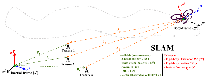
Figure 1: SLAM estimation problem.

Let $R\in\mathbb{SO}\left(3\right)$ be the orientation of a rigid-body and $P\in\mathbb{R}^{3}$ be its translation into 3D space where $R\in\left\{\mathcal{B}\right\}$ and $P\in\left\{\mathcal{I}\right\}$. Assume that the map has $n$ features with ${\rm p}_{i}$ being the $i$th feature location for all $i=1,2,\ldots,n$, and ${\rm p}_{i}\in\left\{\mathcal{I}\right\}$. Let $X=(\boldsymbol{T},\overline{{\rm p}})\in\mathbb{SLAM}_{n}\left(3\right)$ represent the true pose of the rigid-body similar to (1) and features $\overline{{\rm p}}=[\overline{{\rm p}}_{1},\overline{{\rm p}}_{2},\ldots,\overline{{\rm p}}_{n}]\in\overline{\mathcal{M}}^{n}$ where $X$ is unknown. Let $\mathcal{Y}=(\left[U\right]_{\wedge},\overset{\circ}{{\rm v}})\in\mathfrak{slam}_{n}\left(3\right)$ represent the true group velocity that is continuous and bounded such that $\overset{\circ}{{\rm v}}=[\overset{\circ}{{\rm v}}_{1},\overset{\circ}{{\rm v}}_{2},\ldots,\overset{\circ}{{\rm v}}_{n}]\in\overset{\circ}{\mathcal{M}}^{n}$, and assume that $\mathcal{Y}$ measurements are readily available. Therefore, from (1), the true motion dynamics of the rigid-body pose and $n$-features can be expressed as

$$\begin{cases}\dot{\boldsymbol{T}}&=\boldsymbol{T}\left[U\right]_{\wedge}\\ \dot{{\rm p}}_{i}&=R{\rm v}_{i},\hskip 10.00002pt\forall i=1,2,\ldots,n\end{cases}$$ (12)

or, to put simply,

$$\begin{cases}\dot{R}&=R\left[\Omega\right]_{\times}\\ \dot{P}&=RV\\ \dot{{\rm p}}_{i}&=R{\rm v}_{i},\hskip 10.00002pt\forall i=1,2,\ldots,n\end{cases}$$

where $U=\left[\Omega^{\top},V^{\top}\right]^{\top}\in\mathbb{R}^{6}$ denotes the group velocity vector, $\Omega\in\mathbb{R}^{3}$ and $V\in\mathbb{R}^{3}$ stand for the true angular and translational velocity of the rigid-body expressed in the body-frame, respectively, while ${\rm v}_{i}\in\mathbb{R}^{3}$ represents the $i$th linear velocity of a feature expressed in the body-frame such that $\Omega,V,{\rm v}_{i}\in\left\{\mathcal{B}\right\}$. As has been previously discussed and in accordance with Fig. 1, $\boldsymbol{T}\in\mathbb{SE}\left(3\right)$ and $\overline{{\rm p}}\in\overline{\mathcal{M}}^{n}$ are unknown. However, the rigid-body (vehicle) is equipped with multiple sensors that provide us with a set of measurements. The measurements of angular and translational velocity are given by [2, 4]

$$\begin{cases}\Omega_{m}&=\Omega+b_{\Omega}+n_{\Omega}\in\mathbb{R}^{3}\\ V_{m}&=V+b_{V}+n_{V}\in\mathbb{R}^{3}\end{cases}$$ (13)

with $b_{\star}$ and $n_{\star}$ being unknown constant bias and random noise, respectively, associated with the $\star$ element. Let $U_{m}=\left[\Omega_{m}^{\top},V_{m}^{\top}\right]^{\top}$, $b_{U}=\left[b_{\Omega}^{\top},b_{V}^{\top}\right]^{\top}$, and $n_{U}=\left[n_{\Omega}^{\top},n_{V}^{\top}\right]^{\top}$ for all $U_{m},b_{U},n_{U}\in\mathbb{R}^{6}$ and $U_{m},b_{U},n_{U}\in\left\{\mathcal{B}\right\}$. Under the assumption of a static environment adopted in this paper, $\dot{{\rm p}}_{i}=\underline{\mathbf{0}}_{3}$ and entails that ${\rm v}_{i}=\underline{\mathbf{0}}_{3}$ $\forall i=1,2,\ldots,n$. The body-frame measurements associated with the orientation determination can be expressed as [23, 24]

$$\overset{\circ}{a}_{j}=\boldsymbol{T}^{-1}\overset{\circ}{r}_{j}+\overset{\circ}{b}_{j}^{a}+\overset{\circ}{n}_{j}^{a}\in\overset{\circ}{\mathcal{M}},\hskip 10.00002ptj=1,2,\ldots,n_{R}$$

or, more simply,

$$a_{j}=R^{\top}r_{j}+b_{j}^{a}+n_{j}^{a}\in\mathbb{R}^{3}$$ (14)

where $r_{j}$ is the $j$th known inertial-frame vector, $b_{j}^{a}$ is unknown constant bias, and $n_{j}^{a}$ is unknown random noise. It can be easily found that the inverse of $\boldsymbol{T}$ is $\boldsymbol{T}^{-1}=\left[\begin{array}[]{cc}R^{\top}&-R^{\top}P\\ \underline{\mathbf{0}}_{3}^{\top}&1\end{array}\right]\in\mathbb{SE}\left(3\right)$. In our analysis, it is assumed that $b_{j}^{a}=n_{j}^{a}=\underline{\mathbf{0}}_{3}$. Both $r_{j}$ and $a_{j}$ in (14) can be normalized and utilized to extract the rigid-body’s attitude as

$$\upsilon_{j}^{r}=\frac{r_{j}}{\left\|r_{j}\right\|},\hskip 10.00002pt\upsilon_{j}^{a}=\frac{a_{j}}{\left\|a_{j}\right\|}$$ (15)

Let us group the normalized vectors into the following two sets

$$\begin{cases}\upsilon^{r}&=[\upsilon_{1}^{r},\upsilon_{2}^{r},\ldots,\upsilon_{n_{R}}^{r}]\in\left\{\mathcal{I}\right\}\\ \upsilon^{a}&=[\upsilon_{1}^{a},\upsilon_{2}^{a},\ldots,\upsilon_{n_{R}}^{a}]\in\left\{\mathcal{B}\right\}\end{cases}$$ (16)

Remark 1.

The orientation of a rigid-body can be extracted provided that both sets in (16) have a rank of 3, indicating that at least two non-collinear vectors in $\left\{\mathcal{B}\right\}$ and their observations in $\left\{\mathcal{I}\right\}$ are obtainable. The expression in (14) exemplifies two measurements acquired from a low cost IMU and, while the third data point in both $\left\{\mathcal{B}\right\}$ and $\left\{\mathcal{I}\right\}$ can be obtained by means of a cross product $\upsilon_{3}^{a}=\upsilon_{1}^{a}\times\upsilon_{2}^{a}$ and $\upsilon_{3}^{r}=\upsilon_{1}^{r}\times\upsilon_{2}^{r}$, respectively.

Obtaining $n$ features in the body-frame can be done through the utility of low-cost inertial vision units where the $i$th measurement is defined as

$$\overline{y}_{i}=\boldsymbol{T}^{-1}\overline{{\rm p}}_{i}+\overset{\circ}{b}_{i}^{y}+\overset{\circ}{n}_{i}^{y}\in\overline{\mathcal{M}},\hskip 10.00002pt\forall i=1,2,\ldots,n$$

or more simply,

$$y_{i}=R^{\top}({\rm p}_{i}-P)+b_{i}^{y}+n_{i}^{y}\in\mathbb{R}^{3}$$ (17)

where the definitions of $R$, $P$, and ${\rm p}_{i}$ can be found in (12), and $b_{i}^{y}$ and $n_{i}^{y}$ are unknown constant bias and random noise, respectively, for all $y_{i},b_{i}^{y},n_{i}^{y}\in\left\{\mathcal{B}\right\}$. In our analysis, it is assumed that $b_{i}^{y}=n_{i}^{y}=\underline{\mathbf{0}}_{3}$.

Assumption 1.

Assume that the total number of features available for measurement is greater than or equal to 3 which is a necessity for an unambiguous definition of a plane with $\overline{y}=[\overline{y}_{1},\overline{y}_{2},\ldots,\overline{y}_{n}]\in\overline{\mathcal{M}}^{n}$.

IV Nonlinear Filter Design

This section presents two nonlinear filter designs for the SLAM problem. The first nonlinear filter incorporates only the surrounding feature measurements. The second nonlinear filter design considers measurements obtained from a typical low cost IMU in addition to the surrounding feature measurements. Let the estimate of pose be

$$\hat{\boldsymbol{T}}=\left[\begin{array}[]{cc}\hat{R}&\hat{P}\\ \underline{\mathbf{0}}_{3}^{\top}&1\end{array}\right]\in\mathbb{SE}\left(3\right)$$

where $\hat{R}$ and $\hat{P}$ denote estimates of the true orientation and position, respectively. Let $\hat{{\rm p}}_{i}$ be the estimate of the true $i$th feature ${\rm p}_{i}$. Define the error between $\boldsymbol{T}$ and $\hat{\boldsymbol{T}}$ as

$$\tilde{\boldsymbol{T}}=\hat{\boldsymbol{T}}\boldsymbol{T}^{-1} =\left[\begin{array}[]{cc}\hat{R}&\hat{P}\\ \underline{\mathbf{0}}_{3}^{\top}&1\end{array}\right]\left[\begin{array}[]{cc}R^{\top}&-R^{\top}P\\ \underline{\mathbf{0}}_{3}^{\top}&1\end{array}\right]$$ (22)

$$=\left[\begin{array}[]{cc}\tilde{R}&\tilde{P}\\ \underline{\mathbf{0}}_{3}^{\top}&1\end{array}\right]$$ (25)

where $\tilde{R}=\hat{R}R^{\top}$ and $\tilde{P}=\hat{P}-\tilde{R}P$. The objective of pose estimation is to asymptotically drive $\tilde{\boldsymbol{T}}\rightarrow\mathbf{I}_{4}$ which in turn would cause $\tilde{R}\rightarrow\mathbf{I}_{3}$ and $\tilde{P}\rightarrow\underline{\mathbf{0}}_{3}$. To this end, define the error between $\hat{{\rm p}}_{i}$ and ${\rm p}_{i}$ as follows:

$$\overset{\circ}{e}_{i}=\overline{\hat{{\rm p}}}_{i}-\tilde{\boldsymbol{T}}\,\overline{{\rm p}}_{i}\in\overset{\circ}{\mathcal{M}}$$ (26)

where $\overline{\hat{{\rm p}}}_{i}=\left[\hat{{\rm p}}_{i}^{\top},1\right]^{\top}\in\overline{\mathcal{M}}$. In view of (17), $\overset{\circ}{e}_{i}=\overline{\hat{{\rm p}}}_{i}-\hat{\boldsymbol{T}}\boldsymbol{T}^{-1}\,\overline{{\rm p}}_{i}$ can be expressed as

$$\overset{\circ}{e}_{i}=\overline{\hat{{\rm p}}}_{i}-\hat{\boldsymbol{T}}\,\overline{y}_{i}=\left[e_{i}^{\top},0\right]^{\top}$$ (27)

Thus, it can be found that

$$\overset{\circ}{e}_{i} =\left[\begin{array}[]{c}\hat{{\rm p}}_{i}\\ 1\end{array}\right]-\left[\begin{array}[]{cc}\hat{R}&\hat{P}\\ \underline{\mathbf{0}}_{3}^{\top}&1\end{array}\right]\left[\begin{array}[]{c}R^{\top}\left({\rm p}_{i}-P\right)\\ 1\end{array}\right]$$ (34)

$$=\left[\begin{array}[]{c}\tilde{{\rm p}}_{i}-\tilde{P}\\ 0\end{array}\right]$$ (37)

where $\tilde{{\rm p}}_{i}=\hat{{\rm p}}_{i}-\tilde{R}{\rm p}_{i}$ and $\tilde{P}=\hat{P}-\tilde{R}P$. Consider $n_{\Omega}=n_{V}=\underline{\mathbf{0}}_{3}$ and for the group velocity in (13), let the estimate of the unknown bias $b_{U}$ be $\hat{b}_{U}=\left[\hat{b}_{\Omega}^{\top},\hat{b}_{V}^{\top}\right]^{\top}$. Define the error between $b_{U}$ and $\hat{b}_{U}$ as

$$\begin{cases}\tilde{b}_{\Omega}&=b_{\Omega}-\hat{b}_{\Omega}\\ \tilde{b}_{V}&=b_{V}-\hat{b}_{V}\end{cases}$$ (38)

where $\tilde{b}_{U}=\left[\tilde{b}_{\Omega}^{\top},\tilde{b}_{V}^{\top}\right]^{\top}\in\mathbb{R}^{6}$. Before proceeding, it is important to emphasize that the true SLAM dynamics in (12) are nonlinear and are modeled on the Lie group of $\mathbb{SLAM}_{n}\left(3\right)=\mathbb{SE}\left(3\right)\times\overline{\mathcal{M}}^{n}$ with a tangent space of $\mathfrak{slam}_{n}\left(3\right)=\mathfrak{se}\left(3\right)\times\overset{\circ}{\mathcal{M}}^{n}$ where $X=(\boldsymbol{T},\overline{{\rm p}})\in\mathbb{SLAM}_{n}\left(3\right)$ and $\mathcal{Y}=(\left[U\right]_{\wedge},\overset{\circ}{{\rm v}})\in\mathfrak{slam}_{n}\left(3\right)$. It thus follows logically that an efficient SLAM filter should be designed to imitate the nonlinearity of the true SLAM problem by modeling it on the Lie group of $\mathbb{SLAM}_{n}\left(3\right)$ with a tangent space $\mathfrak{slam}_{n}\left(3\right)$. Accordingly, the proposed filter has the structure of $\hat{X}=(\hat{\boldsymbol{T}},\overline{\hat{{\rm p}}})\in\mathbb{SLAM}_{n}\left(3\right)$ and $\hat{\mathcal{Y}}=([\hat{U}]_{\wedge},\overset{\circ}{\hat{{\rm v}}})\in\mathfrak{slam}_{n}\left(3\right)$ where $\hat{\boldsymbol{T}}\in\mathbb{SE}\left(3\right)$ and $\overline{\hat{{\rm p}}}=[\overline{\hat{{\rm p}}}_{1},\ldots,\overline{\hat{{\rm p}}}_{n}]\in\overline{\mathcal{M}}^{n}$ are the pose and feature estimates, respectively, while $\hat{U}\in\mathfrak{se}\left(3\right)$ and $\overset{\circ}{\hat{{\rm v}}}=[\overset{\circ}{\hat{{\rm v}}}_{1},\ldots,\overset{\circ}{\hat{{\rm v}}}_{n}]\in\overset{\circ}{\mathcal{M}}^{n}$ are velocities to be designed in the subsequent subsections. Additionally note that, $\overset{\circ}{\hat{{\rm v}}}_{i}=[\hat{{\rm v}}_{i}^{\top},0]\in\overset{\circ}{\mathcal{M}}$ and $\overline{\hat{{\rm p}}}_{i}=\left[\hat{{\rm p}}_{i}^{\top},1\right]^{\top}\in\overline{\mathcal{M}}$ for all $i=1,2,\cdots,n$.

IV-A Nonlinear Filter Design without IMU

This subsection presents a SLAM nonlinear filter design that operates based solely on measurements obtained from the surrounding features along with angular and translational velocities. Consider the following nonlinear filter evolved directly on $\mathbb{SLAM}_{n}\left(3\right)$:

$$\dot{\hat{\boldsymbol{T}}} =\hat{\boldsymbol{T}}\left[U_{m}-\hat{b}_{U}-W_{U}\right]_{\wedge}$$ (39)

$$W_{U} =-\sum_{i=1}^{n}k_{w}\overline{{\rm Ad}}_{\hat{\boldsymbol{T}}^{-1}}\left[\begin{array}[]{c}\left[\hat{R}y_{i}+\hat{P}\right]_{\times}\\ \mathbf{I}_{3}\end{array}\right]e_{i}$$ (42)

$$\dot{\hat{b}}_{U} =-\sum_{i=1}^{n}\frac{\Gamma}{\alpha_{i}}\overline{{\rm Ad}}_{\hat{\boldsymbol{T}}}^{\top}\left[\begin{array}[]{c}\left[\hat{R}y_{i}+\hat{P}\right]_{\times}\\ \mathbf{I}_{3}\end{array}\right]e_{i}$$ (45)

$$\dot{{\rm\hat{p}}}_{i} =-k_{1}e_{i},\hskip 10.00002pti=1,2,\ldots,n$$ (46)

where $k_{w}$, $k_{1}$, $\Gamma$, and $\alpha_{i}$ are positive constants, $e_{i}$ is as defined in (27), and $\overline{{\rm Ad}}_{\hat{\boldsymbol{T}}}=\left[\begin{array}[]{cc}\hat{R}&0_{3\times 3}\\ {}[\hat{P}]_{\times}\hat{R}&\hat{R}\end{array}\right]$ for all $i=1,2,\cdots,n$. Also, $W_{U}=\left[W_{\Omega}^{\top},W_{V}^{\top}\right]^{\top}\in\mathbb{R}^{6}$ is a correction factor and $\hat{b}_{U}=\left[\hat{b}_{\Omega}^{\top},\hat{b}_{V}^{\top}\right]^{\top}\in\mathbb{R}^{6}$ is the estimate of $b_{U}$.

Theorem 1.

Consider combining the SLAM dynamics $\dot{X}=(\dot{\boldsymbol{T}},\dot{\overline{{\rm p}}})$ in (12) with feature measurements (output $\overline{y}_{i}=\boldsymbol{T}^{-1}\overline{{\rm p}}_{i}$) for all $i=1,2,\ldots,n$ and the velocity measurements ($U_{m}=U+b_{U}$). Let Assumption 1 hold. Let the filter design in (39), (42), (45), and (46) be coupled with the measurements of $U_{m}$ and $\overline{y}_{i}$. Consider the design parameters $k_{w}$, $k_{1}$, $\Gamma$, and $\alpha_{i}$ to be positive constants for all $i=1,2,\ldots,n$, and define the set

$$\mathcal{S}= \left\{(e_{1},e_{2},\ldots,e_{n})\in\mathbb{R}^{3}\times\mathbb{R}^{3}\times\cdots\times\mathbb{R}^{3}\right|$$

$$\hskip 100.00015pt\left.e_{i}=\underline{\mathbf{0}}_{3}\forall i=1,2,\ldots,n\right\}$$ (47)

Then, 1) the error $e_{i}$ in (26) converges exponentially to $\mathcal{S}$, 2) the trajectory of $\tilde{\boldsymbol{T}}$ remains bounded and 3) there exist constants $R_{c}\in\mathbb{SO}\left(3\right)$ and $P_{c}\in\mathbb{R}^{3}$ such that $\tilde{R}\rightarrow R_{c}$ and $\tilde{P}\rightarrow P_{c}$ as $t\rightarrow\infty$.

Proof.

Considering the fact that $\boldsymbol{\dot{T}}^{-1}=-\boldsymbol{T}^{-1}\boldsymbol{\dot{T}}\boldsymbol{T}^{-1}$ and coupling it with the adjoint map in (6), the error dynamics of $\tilde{\boldsymbol{T}}$ defined in (25) can be expressed as below

$$\dot{\tilde{\boldsymbol{T}}} =\dot{\hat{\boldsymbol{T}}}\boldsymbol{T}^{-1}+\hat{\boldsymbol{T}}\dot{\boldsymbol{T}}^{-1}$$

$$=\hat{\boldsymbol{T}}\left[U+\tilde{b}_{U}-W_{U}\right]_{\wedge}\boldsymbol{T}^{-1}-\hat{\boldsymbol{T}}\left[U\right]_{\wedge}\boldsymbol{T}^{-1}$$

$$={\rm Ad}_{\hat{\boldsymbol{T}}}\left(\left[\tilde{b}_{U}-W_{U}\right]_{\wedge}\right)\tilde{\boldsymbol{T}}$$ (48)

Hence, the error dynamics of $\overset{\circ}{e}_{i}$ in (26) become

$$\overset{\circ}{\dot{e}}_{i} =\overset{\circ}{\dot{\hat{{\rm p}}}}_{i}-\dot{\tilde{\boldsymbol{T}}}\,\overline{{\rm p}}_{i}-\tilde{\boldsymbol{T}}\,\dot{\overline{{\rm p}}}_{i}$$

$$=\overset{\circ}{\dot{\hat{{\rm p}}}}_{i}-{\rm Ad}_{\hat{\boldsymbol{T}}}\left(\left[\tilde{b}_{U}-W_{U}\right]_{\wedge}\right)\tilde{\boldsymbol{T}}\,\overline{{\rm p}}_{i}$$ (49)

Recalling the adjoint expressions in (6), (7), and (8), one finds

$${\rm Ad}_{\hat{\boldsymbol{T}}}\left(\left[\tilde{b}_{U}-W_{U}\right]_{\wedge}\right)=\left[\overline{{\rm Ad}}_{\hat{\boldsymbol{T}}}(\tilde{b}_{U}-W_{U})\right]_{\wedge}$$

$$\hskip 50.00008pt=\left[\left[\begin{array}[]{cc}\hat{R}&0_{3\times 3}\\ {}[\hat{P}]_{\times}\hat{R}&\hat{R}\end{array}\right]\left[\begin{array}[]{c}\tilde{b}_{\Omega}-W_{\Omega}\\ \tilde{b}_{V}-W_{V}\end{array}\right]\right]_{\wedge}$$

According to the above result, one obtains

$${\rm Ad}_{\hat{\boldsymbol{T}}}\left(\left[\tilde{b}_{U}-W_{U}\right]_{\wedge}\right)\tilde{\boldsymbol{T}}\,\overline{{\rm p}}_{i}$$

$$\hskip 30.00005pt=\left[\begin{array}[]{cc}\left[\hat{R}y_{i}+\hat{P}\right]_{\times}&\underline{\mathbf{0}}_{3}\\ \mathbf{I}_{3}&\underline{\mathbf{0}}_{3}\end{array}\right]^{\top}\overline{{\rm Ad}}_{\hat{\boldsymbol{T}}}\left(\tilde{b}_{U}-W_{U}\right)$$ (52)

Therefore, one can rewrite the expression in (49) as

$$\overset{\circ}{\dot{e}}_{i} =\overset{\circ}{\dot{\hat{{\rm p}}}}_{i}-\left[\begin{array}[]{cc}\left[\hat{R}y_{i}+\hat{P}\right]_{\times}&\underline{\mathbf{0}}_{3}\\ \mathbf{I}_{3}&\underline{\mathbf{0}}_{3}\end{array}\right]^{\top}\overline{{\rm Ad}}_{\hat{\boldsymbol{T}}}\left(\tilde{b}_{U}-W_{U}\right)$$

Since the last row consists of zeros, the above expression becomes

$$\dot{e}_{i} =\dot{\hat{{\rm p}}}_{i}-\left[\begin{array}[]{c}[\hat{R}y_{i}+\hat{P}]_{\times}\\ \mathbf{I}_{3}\end{array}\right]^{\top}\overline{{\rm Ad}}_{\hat{\boldsymbol{T}}}\left(\tilde{b}_{U}-W_{U}\right)$$ (55)

Define the following candidate Lyapunov function $\mathcal{L}=\mathcal{L}(e_{1},e_{2},\ldots,e_{n},\tilde{b}_{U})$

$$\mathcal{L}=\sum_{i=1}^{n}\frac{1}{2\alpha_{i}}e_{i}^{\top}e_{i}+\frac{1}{2}\tilde{b}_{U}^{\top}\Gamma^{-1}\tilde{b}_{U}$$ (56)

The time derivative of (56) becomes

$$\dot{\mathcal{L}}= \sum_{i=1}^{n}\frac{1}{\alpha_{i}}e_{i}^{\top}\dot{e}_{i}-\tilde{b}_{U}^{\top}\Gamma^{-1}\dot{\hat{b}}_{U}$$

$$= -\sum_{i=1}^{n}\frac{1}{\alpha_{i}}e_{i}^{\top}\left[\begin{array}[]{c}[\hat{R}y_{i}+\hat{P}]_{\times}\\ \mathbf{I}_{3}\end{array}\right]^{\top}\overline{{\rm Ad}}_{\hat{\boldsymbol{T}}}\left(\tilde{b}_{U}-W_{U}\right)$$ (59)

$$+\sum_{i=1}^{n}\frac{1}{\alpha_{i}}e_{i}^{\top}\dot{\hat{{\rm p}}}_{i}-\tilde{b}_{U}^{\top}\Gamma^{-1}\dot{\hat{b}}_{U}$$ (60)

Substituting $W_{U}$, $\dot{\hat{b}}_{U}$ and $\dot{\hat{{\rm p}}}_{i}$ with their definitions in (42), (45), and (46), respectively, results in the following expression:

$$\dot{\mathcal{L}}= -\sum_{i=1}^{n}\frac{k_{1}}{\alpha_{i}}||e_{i}||^{2}-k_{w}\sum_{i=1}^{n}||e_{i}/\alpha_{i}||^{2}$$

$$-k_{w}\left\|\sum_{i=1}^{n}\left[\hat{R}y_{i}+\hat{P}\right]_{\times}\frac{e_{i}}{\alpha_{i}}\right\|^{2}$$ (61)

Consistently with the result obtained in (61) the derivative of $\mathcal{L}$ is negative definite with $\dot{\mathcal{L}}$ being zero at $e_{i}=\underline{\mathbf{0}}_{3}$. Therefore, the result in (61) ensures that $e_{i}$ converges exponentially to the set $\mathcal{S}$ defined in (47). On the basis of Barbalat Lemma, $\dot{\mathcal{L}}$ is negative, continuous and converges to zero. Thus, $\tilde{\boldsymbol{T}}$ and $\tilde{b}_{U}$ remains bounded as well as $\ddot{e}_{i}$. Moreover, according to (37), $e_{i}\rightarrow\underline{\mathbf{0}}_{3}$ implies that $\tilde{{\rm p}}_{i}-\tilde{P}\rightarrow\underline{\mathbf{0}}_{3}$ which in turn, based on (26), leads to $\overline{\hat{{\rm p}}}_{i}-\tilde{\boldsymbol{T}}\,\overline{{\rm p}}_{i}\rightarrow\underline{\mathbf{0}}_{3}$. Therefore, $\tilde{\boldsymbol{T}}$ is bounded, while $\tilde{R}\rightarrow R_{c}$ and $\tilde{P}\rightarrow P_{c}$ as $t\rightarrow\infty$. This completes the proof.∎

Let $\Delta t$ denote a small sample time. Algorithm 1 presents the complete steps of implementation of the continuous filter in (39)-(46) in discrete form. $\exp$ in Algorithm 1 denotes exponential of a matrix which is defined in MATLAB as “expm”.

Algorithm 1 Discrete nonlinear filter for SLAM without IMU described in Subsection IV-A

Initialization:

1. Set $\hat{R}[0]\in\mathbb{SO}\left(3\right)$ and $\hat{P}[0]\in\mathbb{R}^{3}$. Instead, construct $\hat{R}[0]\in\mathbb{SO}\left(3\right)$ using one method of attitude determination, visit [27]

2. Set ${\rm\hat{p}}_{i}[0]\in\mathbb{R}^{3}$ for all $i=1,2,\ldots,n$

3. Set $\hat{b}_{U}[0]=0_{6\times 1}$

4. Select $k_{w}$, $k_{1}$, $\Gamma$, and $\alpha_{i}$ as positive constants, and the sample $k=0$

while

1. $\overline{{\rm Ad}}_{\hat{\boldsymbol{T}}^{-1}}=\left[\begin{array}[]{cc}\hat{R}[k]^{\top}&0_{3\times 3}\\ -\hat{R}[k]^{\top}\left[\hat{P}[k]\right]_{\times}&\hat{R}[k]^{\top}\end{array}\right]$ and
   $\overline{{\rm Ad}}_{\hat{\boldsymbol{T}}}^{\top}=\left[\begin{array}[]{cc}\hat{R}[k]^{\top}&-\hat{R}[k]^{\top}\left[\hat{P}[k]\right]_{\times}\\ 0_{3\times 3}&\hat{R}[k]^{\top}\end{array}\right]$

2. for $i=1:n$

3. $e_{i}[k]=\hat{{\rm p}}_{i}[k]-\hat{R}[k]y_{i}[k]-\hat{P}[k]$ as in (27)

4. end for

5. /* Filter design & update step */

6. $W_{U}[k]=-\sum_{i=1}^{n}k_{w}\overline{{\rm Ad}}_{\hat{\boldsymbol{T}}^{-1}}\left[\begin{array}[]{c}\left[\hat{R}[k]y_{i}[k]+\hat{P}[k]\right]_{\times}\\ \mathbf{I}_{3}\end{array}\right]e_{i}[k]$

7. $\hat{\boldsymbol{T}}[k+1]=\hat{\boldsymbol{T}}[k]\exp\left([U_{m}[k]-\hat{b}_{U}[k]-W_{U}[k]]_{\wedge}\Delta t\right)$

8. $\hat{b}_{U}[k+1]=\hat{b}_{U}[k]$
   $-\sum_{i=1}^{n}\frac{\Gamma\Delta t}{\alpha_{i}}\overline{{\rm Ad}}_{\hat{\boldsymbol{T}}}^{\top}\left[\begin{array}[]{c}\left[\hat{R}[k]y_{i}[k]+\hat{P}[k]\right]_{\times}\\ \mathbf{I}_{3}\end{array}\right]e_{i}[k]$

9. for $i=1:n$

10. ${\rm\hat{p}}_{i}[k+1]={\rm\hat{p}}_{i}[k]-\Delta tk_{1}e_{i}[k]$

11. end for

12. $k=k+1$

end while

IV-B Nonlinear Filter Design with IMU

The nonlinear filter design presented in Subsection IV-A allows $\overset{\circ}{e}_{i}\rightarrow\underline{\mathbf{0}}_{4}$ causing $\tilde{{\rm p}}_{i}-\tilde{P}\rightarrow\underline{\mathbf{0}}_{3}$ exponentially. However, $\tilde{R}\rightarrow R_{c}$ and $\tilde{P}\rightarrow P_{c}$ as $t\rightarrow\infty$ such that $R_{c}\in\mathbb{SO}\left(3\right)$ and $P_{c}\in\mathbb{R}^{3}$ are constants. Recall that $\tilde{P}=\hat{P}-\tilde{R}P$ and $\tilde{{\rm p}}_{i}=\hat{{\rm p}}_{i}-\tilde{R}{\rm p}_{i}$. Accordingly, if the initial pose of the rigid-body ($R\left(0\right)$ and $P\left(0\right)$) is not accurately known, despite $\overset{\circ}{e}_{i}\rightarrow\underline{\mathbf{0}}_{4}$ exponentially, the error between the following pairs of values will be very significant: $\hat{R}\left(\infty\right)$ and $R\left(\infty\right)$, $\hat{P}\left(\infty\right)$ and $P\left(\infty\right)$, and $\hat{{\rm p}}_{i}\left(\infty\right)$ and ${\rm p}_{i}\left(\infty\right)$. As such, the estimates of pose and feature positions will be highly inaccurate. This is the case in previously proposed solutions, for instance [9, 12].

Remark 2.

SLAM problem is not observable [28]. Let $R_{c}\in\mathbb{SO}\left(3\right)$ and $P_{c}\in\mathbb{R}^{3}$ be constants. The best achievable result is $\tilde{R}\rightarrow R_{c}$, $\tilde{P}\rightarrow P_{c}$, and $\hat{{\rm p}}_{i}\rightarrow\hat{P}+\tilde{R}{\rm p}_{i}-\tilde{R}P$ as $t\rightarrow\infty$.

Motivated by the above discussion, this section aims to propose a nonlinear SLAM filter design that demonstrates reasonable performance irrespective of the accuracy of the initial pose and feature locations. The proposed design makes use of the available velocity, IMU, and feature measurements. Recall the body-frame measurements in (14) and their normalization in (15). Let

$$M=M^{\top}=\sum_{j=1}^{n_{{\rm R}}}s_{j}\upsilon_{j}^{r}\left(\upsilon_{j}^{r}\right)^{\top},\hskip 10.00002pt\forall j=1,2,\ldots,n_{{\rm R}}$$ (62)

where $s_{j}\geq 0$ stands for a constant gain and represents the confidence level of the $j$th sensor measurements. According to (62), $M$ is symmetric. In consistence with Remark 1, it is assumed that there are at least two body-frame measurements and their inertial-frame observations are available as well as non-collinear. Thereby, ${\rm rank}(M)=3$. Let the eigenvalues of $M$ be $\lambda(M)=\{\lambda_{1},\lambda_{2},\lambda_{3}\}$. Hence, each eigenvalue is positive. Define $\breve{\mathbf{M}}={\rm Tr}\{M\}\mathbf{I}_{3}-M$, provided that ${\rm rank}(M)=3$. Thus, ${\rm rank}(\breve{\mathbf{M}})=3$ and it can be concluded that ([29] page. 553):

1. $\breve{\mathbf{M}}$ is positive-definite.

2. $\breve{\mathbf{M}}$ has the following eigenvalues $\lambda(\breve{\mathbf{M}})=\{\lambda_{3}+\lambda_{2},\lambda_{3}+\lambda_{1},\lambda_{2}+\lambda_{1}\}$ where the minimum eigenvalue (singular value) $\underline{\lambda}(\breve{\mathbf{M}})>0$.

The rest of this subsection assumes that ${\rm rank}\left(M\right)=3$. Also, for $j=1,2,\ldots,n_{{\rm R}}$, $s_{j}$ is selected such that $\sum_{j=1}^{n_{{\rm R}}}s_{j}=3$. This means that ${\rm Tr}\left\{M\right\}=3$. The following Lemma will prove useful in the reminder of this subsection.

Lemma 1.

Let $\tilde{R}\in\mathbb{SO}\left(3\right)$, $M=M^{\top}\in\mathbb{R}^{3\times 3}$ with ${\rm rank}(M)=3$ and ${\rm Tr}\{M\}=3$. Let $\breve{\mathbf{M}}={\rm Tr}\{M\}\mathbf{I}_{3}-M$ and $\underline{\lambda}=\underline{\lambda}(\breve{\mathbf{M}})$ denote the minimum singular value of $\breve{\mathbf{M}}$. Then, one has

$$||\tilde{R}M||_{{\rm I}} \leq\frac{2}{\underline{\lambda}}\frac{||\mathbf{vex}\left(\boldsymbol{\mathcal{P}}_{a}(\tilde{R}M)\right)||^{2}}{1+{\rm Tr}\{\tilde{R}MM^{-1}\}}$$ (63)

Proof. See [24].

Definition 1.

Define $\mathcal{U}_{s}$ as a subset of $\mathbb{SO}\left(3\right)$ which is a non-attractive and forward invariant unstable set such that

$$\mathcal{U}_{s}=\left\{\left.\tilde{R}\left(0\right)\in\mathbb{SO}\left(3\right)\right|{\rm Tr}\{\tilde{R}\left(0\right)\}=-1\right\}$$ (64)

with $\tilde{R}\left(0\right)={\rm diag}(1,-1,-1)$, $\tilde{R}\left(0\right)={\rm diag}(-1,1,-1)$, or $\tilde{R}\left(0\right)={\rm diag}(-1,-1,1)$ representing the only three possible scenarios for $\tilde{R}\left(0\right)\in\mathcal{U}_{s}$.

The objective of this work is to propose a filter design that relies on a set of measurements. Therefore, it is important to introduce the following variables with respect to vector measurements. Recall (14) and (15). Since the true normalized value of the $j$th body-frame vector is equivalent to $\upsilon_{j}^{a}=R^{\top}\upsilon_{j}^{r}$, define

$$\hat{\upsilon}_{j}^{a}=\hat{R}^{\top}\upsilon_{j}^{r},\hskip 10.00002pt\forall j=1,2,\ldots,n_{{\rm R}}$$ (65)

Let the error in pose be similar to (25) such that $\tilde{R}=\hat{R}R^{\top}$. From the identities in (9) and (10), one obtains

$$\left[\hat{R}\sum_{j=1}^{n_{{\rm R}}}\frac{s_{j}}{2}\hat{\upsilon}_{j}^{a}\times\upsilon_{j}^{a}\right]_{\times} =\hat{R}\sum_{j=1}^{n_{{\rm R}}}\frac{s_{j}}{2}\left(\upsilon_{j}^{a}\left(\hat{\upsilon}_{j}^{a}\right)^{\top}-\hat{\upsilon}_{j}^{a}\left(\upsilon_{j}^{a}\right)^{\top}\right)\hat{R}^{\top}$$

$$=\frac{1}{2}\hat{R}R^{\top}M-\frac{1}{2}MR\hat{R}^{\top}$$

$$=\boldsymbol{\mathcal{P}}_{a}(\tilde{R}M)$$

This implies that $\mathbf{vex}(\boldsymbol{\mathcal{P}}_{a}(\tilde{R}M))$ can be expressed with respect to vector measurements as

$$\boldsymbol{\Upsilon}(\tilde{R}M)=\mathbf{vex}(\boldsymbol{\mathcal{P}}_{a}(\tilde{R}M))=\hat{R}\sum_{j=1}^{n_{{\rm R}}}\left(\frac{s_{j}}{2}\hat{\upsilon}_{j}^{a}\times\upsilon_{j}^{a}\right)$$ (66)

Hence, $\tilde{R}M$ may be expressed in terms of vector measurements as

$$\tilde{R}M=\hat{R}\sum_{j=1}^{n_{{\rm R}}}\left(s_{j}\upsilon_{j}^{a}\left(\upsilon_{j}^{r}\right)^{\top}\right)$$ (67)

Due to the fact that ${\rm Tr}\left\{M\right\}=3$ and in view of the normalized Euclidean distance definition in (5), one finds

$$||\tilde{R}M||_{{\rm I}} =\frac{1}{4}{\rm Tr}\{(\mathbf{I}_{3}-\tilde{R})M\}$$

$$=\frac{1}{4}{\rm Tr}\left\{\mathbf{I}_{3}-\hat{R}\sum_{j=1}^{n_{{\rm R}}}\left(s_{j}\upsilon_{j}^{a}\left(\upsilon_{j}^{r}\right)^{\top}\right)\right\}$$

$$=\frac{1}{4}\sum_{j=1}^{n_{{\rm R}}}\left(1-s_{j}\left(\hat{\upsilon}_{j}^{a}\right)^{\top}\upsilon_{j}^{a}\right)$$ (68)

According to (5), one obtains

$$1-||\tilde{R}||_{{\rm I}} =1-\frac{1}{4}{\rm Tr}\left\{\mathbf{I}_{3}-\tilde{R}\right\}=1-\frac{3}{4}+\frac{1}{4}{\rm Tr}\{\tilde{R}\}$$

$$=\frac{1}{4}\left(1+{\rm Tr}\{\tilde{R}\}\right)$$ (69)

From (69), it becomes apparent that

$$1-||\tilde{R}||_{{\rm I}} =\frac{1}{4}\left(1+{\rm Tr}\{\tilde{R}MM^{-1}\}\right)$$ (70)

From (70) and (67), one has

$$\pi(\tilde{R},M)={\rm Tr}\{\tilde{R}MM^{-1}\}$$

$$\hskip 3.00003pt={\rm Tr}\left\{\left(\sum_{j=1}^{n_{{\rm R}}}s_{j}\upsilon_{j}^{a}\left(\upsilon_{j}^{r}\right)^{\top}\right)\left(\sum_{j=1}^{n_{{\rm R}}}s_{j}\hat{\upsilon}_{j}^{a}\left(\upsilon_{j}^{r}\right)^{\top}\right)^{-1}\right\}$$ (71)

Consider the following nonlinear filter evolved directly on $\mathbb{SLAM}_{n}\left(3\right)$

$$\dot{\hat{\boldsymbol{T}}} =\hat{\boldsymbol{T}}\left[U_{m}-\hat{b}_{U}-W_{U}\right]_{\wedge}$$ (72)

$$\tau_{R} =\underline{\lambda}(\breve{\mathbf{M}})\times(1+\pi(\tilde{R},M))$$ (73)

$$W_{U} =\sum_{i=1}^{n}\frac{1}{\alpha_{i}}\left[\begin{array}[]{cc}\frac{k_{w}\alpha_{i}}{\tau_{R}}\hat{R}^{\top}&0_{3\times 3}\\ 0_{3\times 3}&-k_{2}\hat{R}^{\top}\end{array}\right]\left[\begin{array}[]{c}\boldsymbol{\Upsilon}(\tilde{R}M)\\ e_{i}\end{array}\right]$$ (78)

$$\dot{\hat{b}}_{U} =\sum_{i=1}^{n}\frac{\Gamma}{\alpha_{i}}\left[\begin{array}[]{cc}\frac{\alpha_{i}}{2}\hat{R}^{\top}&-\left[y_{i}\right]_{\times}\hat{R}^{\top}\\ 0_{3\times 3}&-\hat{R}^{\top}\end{array}\right]\left[\begin{array}[]{c}\boldsymbol{\Upsilon}(\tilde{R}M)\\ e_{i}\end{array}\right]$$ (83)

$$\dot{{\rm\hat{p}}}_{i} =-k_{1}e_{i}+\hat{R}\left[y_{i}\right]_{\times}W_{\Omega},\hskip 10.00002pti=1,2,\ldots,n$$ (84)

where $W_{U}=\left[W_{\Omega}^{\top},W_{V}^{\top}\right]^{\top}\in\mathbb{R}^{6}$ is a correction factor and $\hat{b}_{U}=\left[\hat{b}_{\Omega}^{\top},\hat{b}_{V}^{\top}\right]^{\top}\in\mathbb{R}^{6}$ is the estimate of $b_{U}$. $k_{w}$, $k_{1}$, $k_{2}$, $\Gamma=\left[\begin{array}[]{cc}\Gamma_{1}&0_{3\times 3}\\ 0_{3\times 3}&\Gamma_{2}\end{array}\right]$, and $\alpha_{i}$ are positive constants. $M$ is defined in (62), $\pi(\tilde{R},M)$ and $\boldsymbol{\Upsilon}(\tilde{R}M)$ are found in (71) and (66), respectively, while $e_{i}$ is defined in (27) for all $i=1,2,\cdots,n$.

Theorem 2.

Consider the SLAM dynamics $\dot{X}=(\dot{\boldsymbol{T}},\dot{\overline{{\rm p}}})$ in (12) with measurements obtained from features (output $\overline{y}_{i}=\boldsymbol{T}^{-1}\overline{{\rm p}}_{i}$) for all $i=1,2,\ldots,n$, inertial measurement units $\upsilon_{j}^{a}=R^{\top}\upsilon_{j}^{r}$ for all $j=1,2,\ldots,n_{{\rm R}}$ and velocity measurements ($U_{m}=U+b_{U}$). Let Assumption 1 hold along with the discussion in Remark 1 ($n_{{\rm R}}\geq 2$). Assume the filter design to be as in (72), (73), (78), (83), and (84) combined with the measurements $U_{m}$, $\upsilon_{j}^{a}$ and $\overline{y}_{i}$. Consider the design parameters $k_{w}$, $k_{1}$, $k_{2}$, $\Gamma$, and $\alpha_{i}$ to be positive constants for all $i=1,2,\ldots,n$, and $j=1,2,\ldots n_{{\rm R}}$. Define the following set:

$$\mathcal{S}= \left\{(\tilde{R},e_{1},e_{2},\ldots,e_{n})\in\mathbb{SO}\left(3\right)\times\mathbb{R}^{3}\times\mathbb{R}^{3}\times\cdots\times\mathbb{R}^{3}\right|$$

$$\hskip 70.0001pt\left.\tilde{R}=\mathbf{I}_{3},e_{i}=\underline{\mathbf{0}}_{3}\forall i=1,2,\ldots n\right\}$$ (85)

Then, 1) the error $(\tilde{R},e_{1},\ldots,e_{n})$ converges exponentially to $\mathcal{S}$ from almost any initial condition ($\tilde{R}\left(0\right)\notin\mathcal{U}_{s}$), 2) $\tilde{b}_{U}$ converges asymptotically to the origin, and 3) the trajectory of $\tilde{P}$ remains bounded and there exists a constant vector $P_{c}\in\mathbb{R}^{3}$ with $\lim_{t\rightarrow\infty}\tilde{P}=P_{c}$.

Proof.

Since $\dot{\hat{\boldsymbol{T}}}$ in (72) is similar to (39), the pose error dynamics become similar to (48) such that $\dot{\tilde{\boldsymbol{T}}}={\rm Ad}_{\hat{\boldsymbol{T}}}\left(\left[\tilde{b}_{U}-W_{U}\right]_{\wedge}\right)\tilde{\boldsymbol{T}}$. Thus, the attitude error dynamics are

$$\dot{\tilde{R}} =\dot{\hat{R}}R^{\top}+\hat{R}\dot{R}^{\top}=\hat{R}\left[\tilde{b}_{\Omega}-\hat{R}^{\top}W_{\Omega}\right]_{\times}R^{\top}$$

$$=\left[\hat{R}\tilde{b}_{\Omega}-W_{\Omega}\right]_{\times}\tilde{R}$$ (86)

Recall the normalized Euclidean distance definition in (5) such that $||\tilde{R}M||_{{\rm I}}=\frac{1}{4}{\rm Tr}\left\{(\mathbf{I}_{3}-\tilde{R})M\right\}$. Thereby, in view of (11), one has

$$\frac{d}{dt}||\tilde{R}M||_{{\rm I}} =-\frac{1}{4}{\rm Tr}\left\{\left[\hat{R}(\tilde{b}_{\Omega}-W_{\Omega})\right]_{\times}\tilde{R}M\right\}$$

$$=-\frac{1}{4}{\rm Tr}\left\{\tilde{R}M\boldsymbol{\mathcal{P}}_{a}\left(\left[\hat{R}(\tilde{b}_{\Omega}-W_{\Omega})\right]_{\times}\right)\right\}$$

$$=\frac{1}{2}\mathbf{vex}\left(\boldsymbol{\mathcal{P}}_{a}(\tilde{R}M)\right)^{\top}\hat{R}(\tilde{b}_{\Omega}-W_{\Omega})$$ (87)

Note that $\dot{M}=0_{3\times 3}$ by its definition in (62). Recalling the expression in (52), one finds

$${\rm Ad}_{\hat{\boldsymbol{T}}}\left(\left[\tilde{b}_{U}-W_{U}\right]_{\wedge}\right)\tilde{\boldsymbol{T}}\,\overline{{\rm p}}_{i}$$

$$\hskip 30.00005pt=\left[\begin{array}[]{cc}\left[\hat{R}y_{i}+\hat{P}\right]_{\times}&\underline{\mathbf{0}}_{3}\\ \mathbf{I}_{3}&\underline{\mathbf{0}}_{3}\end{array}\right]^{\top}\overline{{\rm Ad}}_{\hat{\boldsymbol{T}}}\left(\tilde{b}_{U}-W_{U}\right)$$ (90)

$$\hskip 30.00005pt=\left[\begin{array}[]{cc}-\hat{R}\left[y_{i}\right]_{\times}&\hat{R}\\ \underline{\mathbf{0}}_{3}^{\top}&\underline{\mathbf{0}}_{3}^{\top}\end{array}\right]\left(\tilde{b}_{U}-W_{U}\right)$$ (93)

Thus, analogously to (55) and in view of (93), the error dynamics of $\overset{\circ}{e}_{i}$ can be expressed as

$$\overset{\circ}{\dot{e}}_{i} =\overset{\circ}{\dot{\hat{{\rm p}}}}_{i}-\left[\begin{array}[]{cc}-\hat{R}\left[y_{i}\right]_{\times}&\hat{R}\\ \underline{\mathbf{0}}_{3}^{\top}&\underline{\mathbf{0}}_{3}^{\top}\end{array}\right]\left(\tilde{b}_{U}-W_{U}\right)$$

which means

$$\dot{e}_{i} =\dot{\hat{{\rm p}}}_{i}-\left[\begin{array}[]{cc}-\hat{R}\left[y_{i}\right]_{\times}&\hat{R}\end{array}\right]\left(\tilde{b}_{U}-W_{U}\right)$$ (95)

Define the following candidate Lyapunov function $\mathcal{L}=\mathcal{L}(e_{1},e_{2},\ldots,e_{n},||\tilde{R}M||_{{\rm I}},\tilde{b}_{U})$

$$\mathcal{L}=\sum_{i=1}^{n}\frac{1}{2\alpha_{i}}e_{i}^{\top}e_{i}+||\tilde{R}M||_{{\rm I}}+\frac{1}{2}\tilde{b}_{U}^{\top}\Gamma^{-1}\tilde{b}_{U}$$ (96)

From (87) and (95), the time derivative of (96) becomes

$$\dot{\mathcal{L}}= \sum_{i=1}^{n}\frac{1}{\alpha_{i}}e_{i}^{\top}\dot{e}_{i}+||\dot{\tilde{R}}M||_{{\rm I}}-\tilde{b}_{U}^{\top}\Gamma^{-1}\dot{\hat{b}}_{U}$$

$$= \sum_{i=1}^{n}\frac{1}{\alpha_{i}}e_{i}^{\top}\dot{\hat{{\rm p}}}_{i}-\sum_{i=1}^{n}\frac{1}{\alpha_{i}}e_{i}^{\top}\left[\begin{array}[]{cc}-\hat{R}\left[y_{i}\right]_{\times}&\hat{R}\end{array}\right](\tilde{b}_{U}-W_{U})$$ (98)

$$+\frac{1}{2}\boldsymbol{\Upsilon}(\tilde{R}M)^{\top}\hat{R}(\tilde{b}_{\Omega}-W_{\Omega})-\tilde{b}_{U}^{\top}\Gamma^{-1}\dot{\hat{b}}_{U}$$ (99)

which means

$$\dot{\mathcal{L}}= \sum_{i=1}^{n}\frac{1}{\alpha_{i}}\left[\begin{array}[]{c}\boldsymbol{\Upsilon}(\tilde{R}M)\\ e_{i}\end{array}\right]^{\top}\left[\begin{array}[]{cc}\frac{\alpha_{i}}{2}\hat{R}&0_{3\times 3}\\ \hat{R}\left[y_{i}\right]_{\times}&-\hat{R}\end{array}\right](\tilde{b}_{U}-W_{U})$$ (104)

$$+\sum_{i=1}^{n}\frac{1}{\alpha_{i}}e_{i}^{\top}\dot{\hat{{\rm p}}}_{i}-\tilde{b}_{U}^{\top}\Gamma^{-1}\dot{\hat{b}}_{U}$$ (105)

With direct substitution of $W_{U}$, $\dot{\hat{b}}_{U}$, and $\dot{\hat{{\rm p}}}_{i}$ with their definitions in (78), (83), and (84), respectively, one obtains

$$\dot{\mathcal{L}}= -\sum_{i=1}^{n}\frac{k_{1}}{\alpha_{i}}||e_{i}||^{2}-\frac{k_{w}}{2\tau_{R}}\left\|\boldsymbol{\Upsilon}(\tilde{R}M)\right\|^{2}-k_{2}\sum_{i=1}^{n}||e_{i}/\alpha_{i}||^{2}$$

As a result of (63) in Lemma 1, one obtains

$$\dot{\mathcal{L}}\leq-\sum_{i=1}^{n}\frac{k_{1}}{\alpha_{i}}||e_{i}||^{2}-\frac{k_{w}}{4}||\tilde{R}M||_{{\rm I}}-k_{2}\sum_{i=1}^{n}||e_{i}/\alpha_{i}||^{2}$$ (106)

According to the result in (106), the derivative of $\dot{\mathcal{L}}$ is negative definite, while $\dot{\mathcal{L}}$ equals to zero at $e_{i}=\underline{\mathbf{0}}_{3}$ as well as $||\tilde{R}M||_{{\rm I}}=0$. By the definition of the normalized Euclidean distance $||\tilde{R}M||_{{\rm I}}=\frac{1}{4}{\rm Tr}\left\{(\mathbf{I}_{3}-\tilde{R})M\right\}$, $||\tilde{R}M||_{{\rm I}}=0$ if and only if $\tilde{R}=\mathbf{I}_{3}$. Thus, the result in (106) ensures that $e_{i}$ as well as $\tilde{R}$ converge exponentially to the set $\mathcal{S}$ defined in (85) for all $i=1,2,\ldots,n$ and $\tilde{R}\left(0\right)\notin\mathcal{U}_{s}$. Based on (63) in Lemma 1 along with the definitions in (68) and (66), $||\tilde{R}M||_{{\rm I}}\rightarrow 0$ implies that $\boldsymbol{\Upsilon}(\tilde{R}M)\rightarrow 0$. $\dot{\mathcal{L}}$ is negative, continuous and converges to zero signifying that $\mathcal{L}\in\mathcal{L}_{\infty}$ and that a finite $\lim_{t\rightarrow\infty}\mathcal{L}$ exists. In view of $\tilde{b}_{U}$ definition in (38) and $\dot{\hat{b}}_{U}$ in (83), $\dot{\tilde{b}}_{U}=-\dot{\hat{b}}_{U}$ implies that $\dot{\tilde{b}}_{U}\rightarrow 0$ as $e_{i}\rightarrow 0$ and $\boldsymbol{\Upsilon}(\tilde{R}M)\rightarrow 0$. Thereby, $\tilde{b}_{U}$ is bounded for all $t\geq 0$. In view of (78), $W_{U}\rightarrow 0$ as $e_{i}\rightarrow 0$ and $\boldsymbol{\Upsilon}(\tilde{R}M)\rightarrow 0$. Moreover, from (84), $\dot{{\rm\hat{p}}}_{i}\rightarrow 0$ as $e_{i}\rightarrow 0$ and $W_{U}\rightarrow 0$. Since $\lim_{t\rightarrow\infty}\dot{e}_{i}=0$ and considering the above discussion, one has

$$\lim_{t\rightarrow\infty}\dot{e}_{i}=\lim_{t\rightarrow\infty}-\left[\begin{array}[]{c}\left[\hat{R}y_{i}+\hat{P}\right]_{\times}\\ \mathbf{I}_{3}\end{array}\right]^{\top}\overline{{\rm Ad}}_{\hat{\boldsymbol{T}}}\tilde{b}_{U}=0$$

Define

$$N=-\left[\begin{array}[]{cc}-\left[\hat{R}y_{1}+\hat{P}\right]_{\times}&\mathbf{I}_{3}\\ \vdots&\vdots\\ -\left[\hat{R}y_{n}+\hat{P}\right]_{\times}&\mathbf{I}_{3}\end{array}\right]\overline{{\rm Ad}}_{\hat{\boldsymbol{T}}}\in\mathbb{R}^{3n\times 6},\hskip 10.00002ptn\geq 3$$

Consistently with Assumption 1, number of features is $n\geq 3$. Accordingly, $N$ is full column rank. It becomes apparent that $\lim_{t\rightarrow\infty}N\tilde{b}_{U}=0$ implies that $\lim_{t\rightarrow\infty}\tilde{b}_{U}=0$. Hence, from (106), $\ddot{\mathcal{L}}$ is bounded. Based on Barbalat Lemma, $\dot{\mathcal{L}}$ is uniformly continuous. Due to the fact that $\tilde{b}_{U}\rightarrow 0$ and $W_{U}\rightarrow 0$ as $t\rightarrow\infty$, $\dot{\tilde{\boldsymbol{T}}}\rightarrow 0$ which leads to $\tilde{\boldsymbol{T}}\rightarrow\boldsymbol{T}_{c}(\mathbf{I}_{3},P_{c})$ with $\boldsymbol{T}_{c}(\mathbf{I}_{3},P_{c})\in\mathbb{SE}\left(3\right)$ denoting a constant matrix where $P_{c}\in\mathbb{R}^{3}$ is a constant vector. Therefore, it can be concluded that $\lim_{t\rightarrow\infty}\tilde{P}=P_{c}$ completing the proof.∎

Remark 3.

Selecting $\tau_{R}=1$ in (73) will lead to

$$\dot{\mathcal{L}}=-\sum_{i=1}^{n}\frac{k_{1}}{\alpha_{i}}||e_{i}||^{2}-\frac{k_{w}}{2}\left\|\boldsymbol{\Upsilon}(\tilde{R}M)\right\|^{2}-k_{2}\sum_{i=1}^{n}||e_{i}/\alpha_{i}||^{2}$$

such that $e_{i}\rightarrow 0$ and $\tilde{R}\rightarrow\mathbf{I}_{3}$ asymptotically for all $i=1,2,\ldots,n$ and $\tilde{R}\left(0\right)\notin\mathcal{U}_{s}$.

Algorithm 2 Discrete nonlinear filter for SLAM described in Subsection IV-B

Initialization:

1. Set $\hat{R}[0]\in\mathbb{SO}\left(3\right)$ and $\hat{P}[0]\in\mathbb{R}^{3}$. Alternatively, construct $\hat{R}[0]\in\mathbb{SO}\left(3\right)$ using one of the methods of attitude determination, visit [27]

2. Set ${\rm\hat{p}}_{i}[0]\in\mathbb{R}^{3}$ for all $i=1,2,\ldots,n$

3. Set $\hat{b}_{U}[0]=0_{6\times 1}$

4. Select $k_{w}$, $k_{1}$, $k_{2}$, $\Gamma$, and $\alpha_{i}$ as positive constants, and the sample $k=0$

while (1) do

1. /* Measurement collection & Filter setup */

2. for $j=1:n_{{\rm R}}$

3. Measurements and observations as in (14)

4. $\upsilon_{j}^{r}=\frac{r_{j}}{\left\|r_{j}\right\|},\upsilon_{j}^{a}=\upsilon_{j}^{a}[k]=\frac{a_{j}[k]}{\left\|a_{j}[k]\right\|}$ as in (15)

5. $\hat{\upsilon}_{j}^{a}=\hat{\upsilon}_{j}^{a}[k]=\hat{R}[k]^{\top}\upsilon_{j}^{r}$ as in (65)

6. end for

7. $M=\sum_{j=1}^{n_{{\rm R}}}s_{j}\upsilon_{j}^{r}\left(\upsilon_{j}^{r}\right)^{\top}$ as in (62) with
   $\breve{\mathbf{M}}={\rm Tr}\left\{M\right\}\mathbf{I}_{3}-M$

8. $\boldsymbol{\Upsilon}=\boldsymbol{\Upsilon}[k]=\hat{R}\sum_{j=1}^{n_{{\rm R}}}(\frac{s_{j}}{2}\hat{\upsilon}_{j}^{a}\times\upsilon_{j}^{a})$ as in (66)

9. $\pi={\rm Tr}\left\{\left(\sum_{j=1}^{n_{{\rm R}}}s_{j}\upsilon_{j}^{a}\left(\upsilon_{j}^{r}\right)^{\top}\right)\left(\sum_{j=1}^{n_{{\rm R}}}s_{j}\hat{\upsilon}_{j}^{a}\left(\upsilon_{j}^{r}\right)^{\top}\right)^{-1}\right\}$ as in (71) where $\pi=\pi[k]$

10. for $i=1:n$

11. $e_{i}[k]=\hat{{\rm p}}_{i}[k]-\hat{R}[k]y_{i}[k]-\hat{P}[k]$ as in (27)

12. end for

13. /* Filter design & update step */

14. $W_{U}[k]=\left[\begin{array}[]{c}W_{\Omega}[k]\\ W_{V}[k]\end{array}\right]=\sum_{i=1}^{n}\frac{1}{\alpha_{i}}\left[\begin{array}[]{c}\frac{k_{w}\alpha_{i}}{\tau_{R}}\hat{R}[k]^{\top}\boldsymbol{\Upsilon}\\ -k_{2}\hat{R}[k]^{\top}e_{i}[k]\end{array}\right]$,
    with $\tau_{R}=\underline{\lambda}(\breve{\mathbf{M}})\times(1+\pi)$

15. $\hat{\boldsymbol{T}}[k+1]=\hat{\boldsymbol{T}}[k]\exp([U_{m}[k]-\hat{b}_{U}[k]-W_{U}[k]]_{\wedge}\Delta t)$

16. $\hat{b}_{U}[k+1]=\hat{b}_{U}[k]$
    $-\sum_{i=1}^{n}\frac{\Gamma\Delta t}{\alpha_{i}}\left[\begin{array}[]{cc}\frac{\alpha_{i}}{2}\hat{R}[k]^{\top}&-\left[y_{i}[k]\right]_{\times}\hat{R}[k]^{\top}\\ 0_{3\times 3}&-\hat{R}[k]^{\top}\end{array}\right]\left[\begin{array}[]{c}\boldsymbol{\Upsilon}\\ e_{i}[k]\end{array}\right]$

17. for $i=1:n$

18. ${\rm\hat{p}}_{i}[k+1]={\rm\hat{p}}_{i}[k]-\Delta t(k_{1}e_{i}[k]+\hat{R}[k]\left[y_{i}[k]\right]_{\times}W_{\Omega}[k])$

19. end for

20. $k=k+1$

end while

The continuous form of the filter proposed in (72)-(84) can be simplified and summarized in terms of vector measurements as follows:

$$\begin{cases}\dot{\hat{R}}&=\hat{R}\left[\Omega_{m}-\hat{b}_{\Omega}-W_{\Omega}\right]_{\times}\\ \dot{\hat{P}}&=\hat{R}(V_{m}-\hat{b}_{V}-W_{V})\\ \tau_{R}&=\underline{\lambda}(\breve{\mathbf{M}})\times(1+\pi(\tilde{R},M))\\ W_{\Omega}&=\frac{k_{w}}{\tau_{R}}\hat{R}^{\top}\boldsymbol{\Upsilon}(\tilde{R}M)\\ W_{V}&=-\sum_{i=1}^{n}\frac{k_{2}}{\alpha_{i}}\hat{R}^{\top}e_{i}\\ \dot{\hat{b}}_{\Omega}&=\frac{\Gamma_{1}}{2}\hat{R}^{\top}\boldsymbol{\Upsilon}(\tilde{R}M)-\sum_{i=1}^{n}\frac{\Gamma_{1}}{\alpha_{i}}[y_{i}]_{\times}\hat{R}^{\top}e_{i}\\ \dot{\hat{b}}_{V}&=-\sum_{i=1}^{n}\frac{\Gamma_{2}}{\alpha_{i}}\hat{R}^{\top}e_{i}\\ \dot{{\rm\hat{p}}}_{i}&=-k_{1}e_{i}+\hat{R}[y_{i}]_{\times}W_{\Omega},\hskip 10.00002pti=1,2,\ldots,n\end{cases}$$ (107)

Let $\Delta t$ denote a small sample time. The detailed implementation steps of the discrete form of the filter proposed in (72)-(84) can be found in Algorithm 2. It should be remarked that $\exp$ in Algorithm 2 denotes exponential of a matrix which is defined in MATLAB as “expm”.

V Simulation Results

In this section, the effectiveness of the proposed nonlinear filter for SLAM on the Lie group $\mathbb{SLAM}_{n}\left(3\right)$ is put to the test. Let the angular velocity be $\Omega=[0,0,0.3]^{\top}({\rm rad/sec})$ and the translational velocity be $V=[2.5,0,0.2t]^{\top}({\rm m/sec})$. Consider the following initial values of the true attitude and position of the vehicle

$$R\left(0\right)=\mathbf{I}_{3},\hskip 10.00002ptP\left(0\right)=[0,0,6]^{\top}$$

Let us place the four features fixed in space relative to the inertial frame at ${\rm p}_{1}=[10,10,0]^{\top}$, ${\rm p}_{2}=[-10,10,0]^{\top}$, ${\rm p}_{3}=[10,-10,0]^{\top}$, and ${\rm p}_{4}=[-10,-10,0]^{\top}$. Suppose that unknown bias is corrupting the group velocity vector $b_{U}=\left[b_{\Omega}^{\top},b_{V}^{\top}\right]^{\top}$ with $b_{\Omega}=[0.2,-0.2,0.2]^{\top}({\rm rad/sec})$ and $b_{V}=[0.04,0.1,-0.02]^{\top}({\rm m/sec})$. In addition, let us assume that the group velocity vector is corrupted with noise defined as $n_{U}=\left[n_{\Omega}^{\top},n_{V}^{\top}\right]^{\top}$ where $n_{\Omega}=\mathcal{N}\left(0,0.2\right)({\rm rad/sec})$ and $n_{V}=\mathcal{N}\left(0,0.2\right)({\rm m/sec})$. Note that $n_{\Omega}=\mathcal{N}\left(0,0.2\right)$ is a short-hand notation for a normally distributed random noise vector with zero mean and a standard deviation of $0.2$. Let two non-collinear inertial-frame observations be given as $r_{1}=\left[1,-1,1\right]^{\top}$ and $r_{2}=\left[0,0,1\right]^{\top}$, and define the body-frame measurements as in (14). In accordance with Remark 1, let us obtain the third observation and the associated measurements by means of a cross product of the two available observations. Let the initial estimates of attitude and position be set to

$$\hat{R}\left(0\right) =\left[\begin{array}[]{ccc}0.8112&-0.5660&0.1468\\ 0.5749&0.8179&-0.0234\\ -0.1068&0.1034&0.9889\end{array}\right]$$

$$\hat{P}\left(0\right) =[0,0,0]^{\top}$$

and suppose that the initial feature position estimates are set to $\hat{{\rm p}}_{1}\left(0\right)=\hat{{\rm p}}_{2}\left(0\right)=\hat{{\rm p}}_{3}\left(0\right)=\hat{{\rm p}}_{4}\left(0\right)=[0,0,0]^{\top}$. Consider the design parameters to be $\alpha_{i}=0.1$, $\Gamma_{1}=3\mathbf{I}_{3}$, $\Gamma_{2}=100\mathbf{I}_{3}$, $k_{w}=5$, $k_{1}=5$, and $k_{2}=20$, with the initial bias estimate being $\hat{b}_{U}\left(0\right)=\underline{\mathbf{0}}_{6}$ for all $i=1,2,3,4$.

The illustration of the true angular and translational velocities plotted against their measurements can be seen in Fig. 2 (two of the three components). Fig. 3 demonstrates evolution of the trajectories estimated by the nonlinear filter for SLAM presented in Subsection IV-B in its continuous form. Although the trajectory of the vehicle was initialized with a large error, Fig. 3 shows how it was smoothly regulated to the true trajectory ultimately reaching the desired destination. Likewise, feature estimates initialized at the origin gradually diverged to their true respective positions.

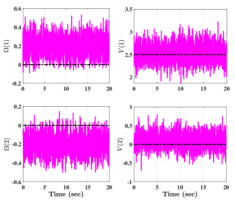
Figure 2: True angular and translational velocities plotted in black center-line vs measurements of angular and translational velocities plotted in magenta solid-line.

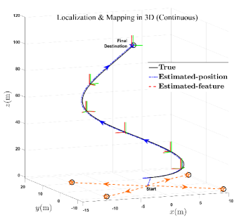
Figure 3: Output trajectories of the proposed nonlinear continuous filter for SLAM described in Subsection IV-B using velocity, feature, and IMU measurements are plotted against the true vehicle and feature positions in 3D space (continuous time). The true vehicle trajectory is depicted in black solid-line with its final destination marked as a black circle. The true orientation of the vehicle is depicted as a green solid-line. Additionally, the true fixed features are marked as black circle at ${\rm p}_{1}$, ${\rm p}_{2}$, ${\rm p}_{3}$, and ${\rm p}_{4}$. The estimation of the travel trajectory is shown as a blue center-line starting from (0,0,0) and ending at its final destination shown as a blue star $\star$. The vehicle orientation estimation is shown as a red solid-line. The estimation process of the feature positions is shown in orange dash-lines which originate at (0,0,0) and end at their final destinations marked with orange stars $\star$.

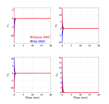
Figure 4: Convergence of the error trajectories of $e_{i}=[e_{i1},e_{i2},e_{i3}]^{\top}$for $i=1,2,3,4$ used in the Lyapunov function candidate. The proposed nonlinear filter for SLAM with IMU described in Subsection IV-B is plotted in blue against the nonlinear filter for SLAM described in Subsection IV-A plotted in red.

Fig. 4 summaries the asymptotic convergence behavior of $e_{i}$ when using the nonlinear SLAM filter with and without IMU for all $i=1,2,3,4$. Recall that $\tilde{R}=\hat{R}R^{\top}$, $\tilde{P}=\hat{P}-\tilde{R}P$, $\tilde{{\rm p}}_{i}=\hat{{\rm p}}_{i}-\tilde{R}{\rm p}_{i}$, and $||\tilde{R}||_{{\rm I}}=\frac{1}{4}{\rm Tr}\{\mathbf{I}_{3}-\tilde{R}\}$. Considering the nonlinear SLAM filter without IMU described in Subsection IV-A one will notice that since $e_{i}=\tilde{{\rm p}}_{i}-\tilde{P}$, asymptotic convergence of $e_{i}$ does not imply that $||\tilde{R}||_{{\rm I}}\rightarrow 0$, $\tilde{P}\rightarrow 0$, and $\tilde{{\rm p}}_{i}\rightarrow 0$. Therefore, it follows that $\tilde{R}$, $\tilde{P}$, and $\tilde{{\rm p}}_{i}$ converge to a constant. However, the real objective of the SLAM filter design is to achieve $||\tilde{R}||_{{\rm I}}\rightarrow 0$, $||P-\hat{P}||\rightarrow 0$, and $||{\rm p}_{i}-{\rm\hat{p}}_{i}||\rightarrow 0$. Fig. 5 compares and contrasts the performance of the proposed nonlinear SLAM filter with IMU and the nonlinear filter without IMU, emphasizing the robustness and effectiveness in presence of IMU. As illustrated in Fig. 5, the nonlinear filter for SLAM without IMU produced poor tracking performance of the error components: $||\tilde{R}||_{{\rm I}}$, $||P-\hat{P}||$, and $||{\rm p}_{i}-{\rm\hat{p}}_{i}||$ in consistence with [9]. In contrast, the proposed nonlinear filter with IMU, also depicted in Fig. 5, demonstrates asymptotic convergence of the attitude error ($||\tilde{R}||_{{\rm I}}$) as well as reasonable convergence of the position error ($||P-\hat{P}||$) and the $i$th feature error ($||{\rm p}_{i}-{\rm\hat{p}}_{i}||$) to the close neighborhood of the origin. Despite the presence of the residual error in $||P-\hat{P}||$ and $||{\rm p}_{i}-{\rm\hat{p}}_{i}||$, remarkable difference is observed in the convergence of $||\tilde{R}||_{{\rm I}}$, $||P-\hat{P}||$, and $||{\rm p}_{i}-{\rm\hat{p}}_{i}||$ between the filter described in Subsection IV-A and the novel filter proposed in Subsection IV-B.

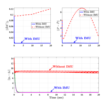
Figure 5: Evolution of the error trajectories of $||\hat{R}R^{\top}||_{{\rm I}}$, $||P-\hat{P}||$, and $||{\rm p}_{i}-{\rm\hat{p}}_{i}||$ for all $i=1,2,3,4$. Blue represents the proposed nonlinear filter that uses velocity, feature, and IMU measurements given in Subsection IV-B, while red corresponds to the nonlinear filter that uses velocity and feature measurements given in Subsection IV-A.

While Fig. 3, 4 and 5 demonstrate the output performance of the proposed continuous filter described in (72)-(84), Fig. 6 presents its discrete counterpart described in Algorithm 2 implemented with a sample time of $\Delta t=0.001$ sec. The simulation of the discrete filter utilizes the same measurements, initialization, and design parameters introduced at the beginning of the Simulation Section with the exception of $V=[2.5,0,0]^{\top}({\rm m/sec})$. Analogously to the continuous filter, Fig. 6 demonstrates the superb tracking performance of the proposed discrete nonlinear observer. In addition, Fig. 6 reveals that the filter is computationally cheap and can be successfully implemented using an inexpensive kit.

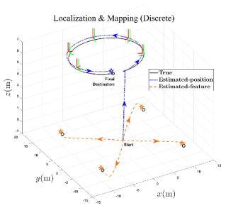
Figure 6: Output trajectories of the proposed nonlinear filter for SLAM described in Algorithm 2. The true vehicle trajectory, and the vehicle and feature final destinations are plotted as a black solid-line, and black circle, respectively. The estimation process of the vehicle’s trajectory, vehicle’s final destination, feature trajectories, and feature final destinations are shown as a blue center-line, a blue star $\star$, orange center-lines, and orange stars $\star$, respectively. The true vehicle orientation is depicted as a green solid-line, while its estimation is plotted as a red solid-line.

To summarize, Fig. 3, 4, 5, and 6 illustrate strong tracking capabilities of the proposed filter to localize the unknown vehicle’s position and simultaneously map the unknown environment.

VI Conclusion

In this paper, the Simultaneous Localization and Mapping (SLAM) problem has been addressed on the Lie group of $\mathbb{SLAM}_{n}\left(3\right)$ mimicking the nonlinear motion dynamics of the true SLAM problem. The proposed nonlinear filter for SLAM evolved directly utilizes on the Lie group of $\mathbb{SLAM}_{n}\left(3\right)$ utilizes the measurements of translational and angular velocity, as well as feature and IMU measurements. The power of the proposed approach consists in its ability to account for the unknown bias inevitably present in velocity measurements. As has been revealed through extensive simulation, the proposed filter exhibits exceptional results by localizing the unknown pose of the vehicle while simultaneously mapping the unknown environment in both discrete and continuous time.

Appendix

Quaternion Representation

Let $Q=[q_{0},q^{\top}]^{\top}\in\mathbb{S}^{3}$ be a unit-quaternion where $q_{0}\in\mathbb{R}$ and $q\in\mathbb{R}^{3}$ such that $\mathbb{S}^{3}=\{\left.Q\in\mathbb{R}^{4}\right|||Q||=\sqrt{q_{0}^{2}+q^{\top}q}=1\}$. $Q^{-1}=[\begin{array}[]{cc}q_{0}&-q^{\top}\end{array}]^{\top}\in\mathbb{S}^{3}$ stands for the inverse of $Q$. Define $\odot$ as a quaternion product, hence, the quaternion multiplication of $Q_{1}=[\begin{array}[]{cc}q_{01}&q_{1}^{\top}\end{array}]^{\top}\in\mathbb{S}^{3}$ and $Q_{2}=[\begin{array}[]{cc}q_{02}&q_{2}^{\top}\end{array}]^{\top}\in\mathbb{S}^{3}$ can be represented as follows:

$$Q_{1}\odot Q_{2}=\left[\begin{array}[]{c}q_{01}q_{02}-q_{1}^{\top}q_{2}\\ q_{01}q_{2}+q_{02}q_{1}+[q_{1}]_{\times}q_{2}\end{array}\right]$$

Unit-quaternion ($\mathbb{S}^{3}$) to $\mathbb{SO}\left(3\right)$ mapping can be expressed as $\mathcal{R}_{Q}:\mathbb{S}^{3}\rightarrow\mathbb{SO}\left(3\right)$

$$\mathcal{R}_{Q} =(q_{0}^{2}-||q||^{2})\mathbf{I}_{3}+2qq^{\top}+2q_{0}\left[q\right]_{\times}\in\mathbb{SO}\left(3\right)$$ (108)

$Q_{{\rm I}}=[\pm 1,0,0,0]^{\top}$ represents the quaternion identity where $\mathcal{R}_{Q_{{\rm I}}}=\mathbf{I}_{3}$. More information can be found in [30]. Define the estimate of $Q=[q_{0},q^{\top}]^{\top}\in\mathbb{S}^{3}$ as $\hat{Q}=[\hat{q}_{0},\hat{q}^{\top}]^{\top}\in\mathbb{S}^{3}$ with

$$\mathcal{R}_{\hat{Q}}=(\hat{q}_{0}^{2}-||\hat{q}||^{2})\mathbf{I}_{3}+2\hat{q}\hat{q}^{\top}+2\hat{q}_{0}\left[\hat{q}\right]_{\times}\in\mathbb{SO}\left(3\right)$$

Recall the map in (108). Define the map

$$\left[\begin{array}[]{c}0\\ \mathbf{Y}(\hat{Q},x)\end{array}\right] =\hat{Q}\odot\left[\begin{array}[]{c}0\\ x\end{array}\right]\odot\hat{Q}^{-1}$$

$$\left[\begin{array}[]{c}0\\ \mathbf{Y}(\hat{Q}^{-1},x)\end{array}\right] =\hat{Q}^{-1}\odot\left[\begin{array}[]{c}0\\ x\end{array}\right]\odot\hat{Q}$$

with $\mathbf{Y}(\hat{Q},y_{i})\in\mathbb{R}^{3}$, $x\in\mathbb{R}^{3}$, and $\hat{Q}\in\mathbb{S}^{3}$. Let us reformulate the observer in (72), (84), (83), and (78) along with its implementation steps in terms of unit-quaternion:

$$\begin{cases}e_{i}&=\hat{{\rm p}}_{i}-\mathbf{Y}\left(\hat{Q},y_{i}\right)-\hat{P},\hskip 10.00002pti=1,2,\ldots,n\\ \boldsymbol{\Upsilon}(\tilde{R}M)&=\mathbf{Y}\left(\hat{Q},\sum_{j=1}^{n_{{\rm R}}}\left(\frac{s_{j}}{2}\hat{\upsilon}_{j}^{a}\times\upsilon_{j}^{a}\right)\right)\\ \tau_{R}&=\underline{\lambda}(\breve{\mathbf{M}})\times(1+\pi(\tilde{R},M))\\ \chi&=\Omega_{m}-\hat{b}_{\Omega}-W_{\Omega}\\ \dot{\hat{Q}}&=\frac{1}{2}\left[\begin{array}[]{cc}0&-\chi^{\top}\\ \chi&-\left[\chi\right]_{\times}\end{array}\right]\hat{Q},\hskip 10.00002pt\hat{Q}(0)=Q_{{\rm I}}\\ \dot{\hat{P}}&=\mathbf{Y}\left(\hat{Q},V_{m}-\hat{b}_{V}-W_{V}\right)\\ \dot{{\rm\hat{p}}}_{i}&=-k_{1}e_{i}+\mathbf{Y}\left(\hat{Q},[y_{i}]_{\times}W_{\Omega}\right)\\ \dot{\hat{b}}_{\Omega}&=\frac{\Gamma_{1}}{2}\mathbf{Y}\left(\hat{Q}^{-1},\boldsymbol{\Upsilon}(\tilde{R}M)\right)\\ &\hskip 10.00002pt-\sum_{i=1}^{n}\frac{\Gamma_{1}}{\alpha_{i}}[y_{i}]_{\times}\mathbf{Y}\left(\hat{Q}^{-1},e_{i}\right)\\ \dot{\hat{b}}_{V}&=-\sum_{i=1}^{n}\frac{\Gamma_{2}}{\alpha_{i}}\mathbf{Y}\left(\hat{Q}^{-1},e_{i}\right)\\ W_{\Omega}&=\frac{k_{w}}{\tau_{R}}\mathbf{Y}\left(\hat{Q}^{-1},\boldsymbol{\Upsilon}(\tilde{R}M)\right)\\ W_{V}&=-\sum_{i=1}^{n}\frac{k_{2}}{\alpha_{i}}\mathbf{Y}\left(\hat{Q}^{-1},e_{i}\right)\end{cases}$$

AUTHOR INFORMATION

Hashim A. Hashim (Member, IEEE) is an Assistant Professor with the Department of Engineering and Applied Science, Thompson Rivers University, Kamloops, British Columbia, Canada. He received the B.Sc. degree in Mechatronics, Department of Mechanical Engineering from Helwan University, Cairo, Egypt, the M.Sc. in Systems and Control Engineering, Department of Systems Engineering from King Fahd University of Petroleum & Minerals, Dhahran, Saudi Arabia, and the Ph.D. in Robotics and Control, Department of Electrical and Computer Engineering at Western University, Ontario, Canada.
His current research interests include stochastic and deterministic attitude and pose filters, Guidance, navigation and control, simultaneous localization and mapping, control of multi-agent systems, and optimization techniques.

Contact Information: hhashim@tru.ca.

Abdelrahman E.E. Eltoukhy received his BSc Degree in Production Engineering from Helwan University, Egypt, and obtained his MSc in Engineering and Management from the Politecnico Di Torino, Italy. He obtained his PhD degree from The Hong Kong Polytechnic University, Hong Kong. He is currently a Research Assistant Professor in Industrial and Systems Engineering department, The Hong Kong Polytechnic University, Hong Kong.
His current research interests include airline schedule planning, logistics and supply chain management, operations research, and simulation.

References

• [1] S. Thrun et al., “Robotic mapping: A survey,” Exploring artificial intelligence in the new millennium, vol. 1, no. 1-35, p. 1, 2002.
• [2] H. A. Hashim, L. J. Brown, and K. McIsaac, “Nonlinear pose filters on the special euclidean group SE(3) with guaranteed transient and steady-state performance,” IEEE Transactions on Systems, Man, and Cybernetics: Systems, pp. 1–14, 2019.
• [3] D. E. Zlotnik and J. R. Forbes, “Higher order nonlinear complementary filtering on lie groups,” IEEE Transactions on Automatic Control, vol. 64, no. 5, pp. 1772–1783, 2018.
• [4] H. A. Hashim and F. L. Lewis, “Nonlinear stochastic estimators on the special euclidean group SE(3) using uncertain imu and vision measurements,” IEEE Transactions on Systems, Man, and Cybernetics: Systems, vol. PP, no. PP, pp. PP–PP, 2020.
• [5] H. Choset, S. Walker, K. Eiamsa-Ard, and J. Burdick, “Sensor-based exploration: Incremental construction of the hierarchical generalized voronoi graph,” The International Journal of Robotics Research, vol. 19, no. 2, pp. 126–148, 2000.
• [6] H. Durrant-Whyte and T. Bailey, “Simultaneous localization and mapping: part i,” IEEE robotics & automation magazine, vol. 13, no. 2, pp. 99–110, 2006.
• [7] K. E. Bekris, M. Glick, and L. E. Kavraki, “Evaluation of algorithms for bearing-only slam,” in Proceedings 2006 IEEE International Conference on Robotics and Automation, 2006. ICRA 2006.   IEEE, 2006, pp. 1937–1943.
• [8] A. J. Davison, I. D. Reid, N. D. Molton, and O. Stasse, “Monoslam: Real-time single camera slam,” IEEE transactions on pattern analysis and machine intelligence, vol. 29, no. 6, pp. 1052–1067, 2007.
• [9] D. E. Zlotnik and J. R. Forbes, “Gradient-based observer for simultaneous localization and mapping,” IEEE Transactions on Automatic Control, vol. 63, no. 12, pp. 4338–4344, 2018.
• [10] Y. Liu, Z. Li, T. Zhang, and S. Zhao, “Brain-robot interface-based navigation control of a mobile robot in corridor environments,” IEEE Transactions on Systems, Man, and Cybernetics: Systems, 2018.
• [11] I. Maurovic, M. Seder, K. Lenac, and I. Petrovic, “Path planning for active slam based on the d* algorithm with negative edge weights,” IEEE Transactions on Systems, Man, and Cybernetics: Systems, vol. 48, no. 8, pp. 1321–1331, 2017.
• [12] H. A. Hashim, “Guaranteed performance nonlinear observer for simultaneous localization and mapping,” IEEE Control Systems Letters, vol. 5, no. 1, pp. 91–96, 2021.
• [13] W. Yuan, Z. Li, and C.-Y. Su, “Multisensor-based navigation and control of a mobile service robot,” IEEE Transactions on Systems, Man, and Cybernetics: Systems, 2019.
• [14] M. Montemerlo and S. Thrun, FastSLAM: A scalable method for the simultaneous localization and mapping problem in robotics.   Springer, 2007, vol. 27.
• [15] M. Kaess, A. Ranganathan, and F. Dellaert, “isam: Incremental smoothing and mapping,” IEEE Transactions on Robotics, vol. 24, no. 6, pp. 1365–1378, 2008.
• [16] S. Huang and G. Dissanayake, “Convergence and consistency analysis for extended kalman filter based slam,” IEEE Transactions on robotics, vol. 23, no. 5, pp. 1036–1049, 2007.
• [17] A. Chatterjee and F. Matsuno, “A neuro-fuzzy assisted extended kalman filter-based approach for simultaneous localization and mapping (slam) problems,” IEEE transactions on fuzzy systems, vol. 15, no. 5, pp. 984–997, 2007.
• [18] T. Zhang, K. Wu, J. Song, S. Huang, and G. Dissanayake, “Convergence and consistency analysis for a 3-d invariant-ekf slam,” IEEE Robotics and Automation Letters, vol. 2, no. 2, pp. 733–740, 2017.
• [19] G. Dissanayake, S. Huang, Z. Wang, and R. Ranasinghe, “A review of recent developments in simultaneous localization and mapping,” in 2011 6th International Conference on Industrial and Information Systems.   IEEE, 2011, pp. 477–482.
• [20] C. Cadena, L. Carlone, H. Carrillo, Y. Latif, D. Scaramuzza, J. Neira, I. Reid, and J. J. Leonard, “Past, present, and future of simultaneous localization and mapping: Toward the robust-perception age,” IEEE Transactions on robotics, vol. 32, no. 6, pp. 1309–1332, 2016.
• [21] T. Lee, “Exponential stability of an attitude tracking control system on so (3) for large-angle rotational maneuvers,” Systems & Control Letters, vol. 61, no. 1, pp. 231–237, 2012.
• [22] H. F. Grip, T. I. Fossen, T. A. Johansen, and A. Saberi, “Attitude estimation using biased gyro and vector measurements with time-varying reference vectors,” IEEE Transactions on Automatic Control, vol. 57, no. 5, pp. 1332–1338, 2012.
• [23] H. A. Hashim, L. J. Brown, and K. McIsaac, “Nonlinear stochastic attitude filters on the special orthogonal group 3: Ito and stratonovich,” IEEE Transactions on Systems, Man, and Cybernetics: Systems, vol. 49, no. 9, pp. 1853–1865, 2019.
• [24] H. A. Hashim, “Systematic convergence of nonlinear stochastic estimators on the special orthogonal group SO(3),” International Journal of Robust and Nonlinear Control, vol. 30, no. 10, pp. 3848–3870, 2020.
• [25] H. Strasdat, “Local accuracy and global consistency for efficient visual slam,” Ph.D. dissertation, Department of Computing, Imperial College London, 2012.
• [26] T. A. Johansen and E. Brekke, “Globally exponentially stable kalman filtering for slam with ahrs,” in 2016 19th International Conference on Information Fusion (FUSION).   IEEE, 2016, pp. 909–916.
• [27] H. A. Hashim, “Attitude determination and estimation using vector observations: Review, challenges and comparative results,” arXiv preprint arXiv:2001.03787, 2020.
• [28] K. W. Lee, W. S. Wijesoma, and J. I. Guzman, “On the observability and observability analysis of slam,” in 2006 IEEE/RSJ International Conference on Intelligent Robots and Systems.   IEEE, 2006, pp. 3569–3574.
• [29] F. Bullo and A. D. Lewis, Geometric control of mechanical systems: modeling, analysis, and design for simple mechanical control systems.   Springer Science & Business Media, 2004, vol. 49.
• [30] H. A. Hashim, “Special orthogonal group SO(3), euler angles, angle-axis, rodriguez vector and unit-quaternion: Overview, mapping and challenges,” arXiv preprint arXiv:1909.06669, 2019.