Identifying Reaction Pathways in Phase Space via Asymptotic Trajectories

Abstract

In this paper, we revisit the concepts of the reactivity map and the reactivity bands as an alternative to the use of perturbation theory for the determination of the phase space geometry of chemical reactions. We introduce a reformulated metric, called the asymptotic trajectory indicator, and an efficient algorithm to obtain reactivity boundaries. We demonstrate that this method has sufficient accuracy to reproduce phase space structures such as turnstiles for a 1D model of the isomerization of ketene in an external field. The asymptotic trajectory indicator can be applied to higher dimensional systems coupled to Langevin baths as we demonstrate for a 3D model of the isomerization of ketene.

I Introduction

The identification of a reaction path (or pathway) has received attention from the beginning of the development of transition state theory (TST)Eyring (1935); Evans and Polanyi (1935); Wigner (1938) to characterize the energetics of the reaction between reactants and products. Eyring called it “the path requiring least energy”Glasstone et al. (1941) which is now commonly called the minimum energy path (MEP) and obtained as the path of least resistance starting from the energy minimum associated with the reactant. Fukui is generally credited for what came to be known as the intrinsic reaction coordinate (IRC)Fukui (1970); Kato and Fukui (1976) because he introduced it, in a mass-weighted coordinate system, as the path of steepest descent starting from the saddle. Beyond the developments in the statistical formulation of TST,Glasstone et al. (1941); Laidler and King (1983); Truhlar et al. (1983); Hänggi et al. (1990); Truhlar et al. (1996) the re-imagination of the reaction path as an object in full phase spaceKeck (1967) led to the use of reactivity bandsWall et al. (1958); Wright (1978) and the periodic orbit dividing surface (PODS)Pollak and Pechukas (1978) to characterize reactions. Both analyses are formulated in terms of identifying the trajectories in between the reactive and non-reactive trajectories. See Ref. Nagahata et al., 2013a for more details, and Ref. Patra and Keshavamurthy, 2018 for the connection to reaction path samplingDellago et al. (1998, 2002) also qualitatively described in our earlier work.Bartsch et al. (2005); Hernandez et al. (2010) We are thus led to use these mathematical structures to reconsider the determination of the optimal reaction path in phase space.

In the 1980s, dynamical system theory was advanced through the use of the Poincaré map,Davis (1984) turnstileMackay et al. (1984) structures, and reaction island theory.Ozorio de Almeida et al. (1990) Unfortunately, all of these methods are applicable mostly to systems up to 2 degrees of freedom (DoF). Going beyond this restriction, WigginsWiggins (1990) suggested a multidimensional generalization of the unstable periodic orbit in 2 DoF systems and the reaction pathway associated with it. The former is NHIM normally hyperbolic invariant manifold (NHIM), and the latter is the boundary of the reaction pathway which can be understood as the stable and unstable manifolds of the NHIM. In the limit of two dimensional systems, the NHIM is an unstable periodic orbit which was later understood as an anchor of the PODS.Wiggins et al. (2001); Hernandez et al. (2010) FenichelFenichel (1972) was the first to prove that these NHIMs persist under perturbation. For simplicity, in this work, we call this and its subsequent generalizations, the NHIM Persistence Theorem (see Appendix A). A consequence of this theorem is that the saddle point on the potential energy surface plays a significant role in many cases because the structure of the NHIM near the energy of the saddle point will persist for larger energies as long as the truncated higher-order terms in perturbation theory are small enough.

The pioneering work on the application of perturbation theory for reaction dynamics in the chemical physics community was made by Hernandez and MillerHernandez and Miller (1993); Hernandez (1994) through Van Vleck semiclassical perturbation theory and by Komatsuzaki et al.Komatsuzaki and Nagaoka (1996) through classical Lie- canonical perturbation theory (CPT) (also known as a component of Birkhoff normal form theory) to obtain non-recrossing dividing surfaces in many DoFs. Uzer et al. Uzer et al. (2002) later showed the relation between this normal form theory and the geometry of the reaction pathway. The normal form theory was also further generalized to address related challenges in quantum systems,Waalkens et al. (2008) the effects under rotational coupling,Kawai and Komatsuzaki (2011a); Çiftçi and Waalkens (2012) Langevin dynamics,Kawai and Komatsuzaki (2009a, b) generalized Langevin dynamics,Kawai and Komatsuzaki (2010a) and the classicalKawai et al. (2007) and the quantumKawai and Komatsuzaki (2011b) dynamics under an external field. The extraction of the transition state (TS) trajectoryBartsch et al. (2005) and relaxation of the normal form theoryLi et al. (2006); Kawai and Komatsuzaki (2010b) plays a crucial role especially in time-dependentKawai et al. (2007); Kawai and Komatsuzaki (2011b) and stochasticBartsch et al. (2006); Kawai and Komatsuzaki (2009a, b, 2010a) theories. Naturally, perturbation theories are limited and are applicable only when the zeroth order approximation (typically normal mode Hamiltonian) is valid, and the asymptotic series returns converged results.

Challenges to this theory arise when the TS or the phase space bottleneck is not strongly dominated by a potential energy saddle point. Perturbation theories expanded around such a point are not expected to be accurate unless the bottleneck happens to remain within the convergence radius of the perturbation.Li et al. (2006) One possible such challenge comes from the existing of the roaming reaction pathway observed experimentally in formaldehyde H2CO decomposition path to H_2 + CO.Townsend et al. (2004); Bowman and Shepler (2011) The phase space manifestation of this systemMauguière et al. (2017) shows the significant role of the reactivity boundary in the absence of a potential energy saddle. Nevertheless, the structure of transition state theory can be preserved even when such roaming reactions are present through the identification and use of a global transition state dividing surfaces.Ulusoy et al. (2013) There are other known examples that the reaction mechanisms are irregular due to factors such as long-time trapping in a well,Davis (1984) bifurcation of the PODS,Pollak and Pechukas (1978); Li et al. (2006) dynamical switching of the reaction coordinate,Teramoto et al. (2011) and the presence of near higher-index saddles,Nagahata et al. (2013b, a) with chemical species shown in the references. In the limit of two or fewer DoFs, there are nonperturbative approaches such as periodic orbit analysis, which is used in an effectively 2 DoF system of the roaming reaction path: H2CO -¿ OC H_2 -¿ H_2 + CO.Mauguière et al. (2017) However, the extension of these approaches to the systems with higher than 2 DoF is still a challenging task.

An alternative approach to determining the reactivity boundary is rooted in the Lagrangian coherent structure (LCS)Haller (2015); Hadjighasem et al. (2017) of the dynamics in the Lagrangian frame. The LCS is mediated by the NHIM and its stable/unstable manifolds, and can be evaluated by numerical analysisHadjighasem et al. (2017) —e.g., through the identification of the finite time Lyapunov exponent (FTLE) ridge. The FTLE analysis has mostly been employed in effectively two-dimensional systems, such as ocean flows due to theoretical and numerical limitations. The Lagrangian descriptor (LD)Mendoza and Mancho (2010) was proposed as a heuristic alternative. In the context of reaction dynamics, the LD was first introduced by Craven and Hernandez.Craven and Hernandez (2015) The theory provides, for example, a way to obtain nonrecrossing dividing surfaces in barrierless reactions in which perturbation theory is nonsensical because no unique zeroth-order dividing surface is available.Junginger and Hernandez (2016) It has also been used to reveal geometric features in molecular systems such as keteneCraven and Hernandez (2016) and LiCN.Revuelta et al. (2019)

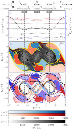
Figure 1: Highlights of the main results of this paper for the 1 D ketene isomerization reaction in an external field: (a) The potential energy $V_{\mathrm{F}}(q_{\mathrm{F}})$ (solid black line), the external force through dipole interaction $V_{\mathrm{ex}}(q_{\mathrm{F}},t)$ at phases $\omega t=n\pi/3$ for $n=3,2,\dots,-3$ (colored dotted lines with values of $V_{\mathrm{ex}}$ shown in the right axis), the TSs (gray plus symbols), the minima (gray filled-circles and vertical dashed lines) corresponding to the chemical formulas (ketene, formylmethylene, and oxirene), and the left (red) and right (blue) absorbing boundaries. (b) The first passage time to the left (right) absorbing boundary $\tau_{\mathrm{f}}^{\mathrm{L}}$ ($\tau_{\mathrm{f}}^{\mathrm{R}}$), or recurrent time after $\omega t=14\pi$ (gray), or ATI with the color scale given at the bottom. They provide the phase space skeleton of the reaction (yellow). (c) The phase space geometry structures shown here for comparison are the stable (blue) and unstable (red) manifolds, and regions whose points exit right (blue) or left (red). A sample trajectory (black dashed line) is shown to illustrate the points on the Poincaré surface of section in corresponding regions: square and circles on the time slice $|\omega t|\equiv 0\pmod{2\pi}$.

In this paper, we propose a non-heuristic approach for locating the reaction pathways in a phase space. The approach is an alternative to the nonperturbative methods cited above. Toward its formulation, we revisit the theory of the reactivity mapWright (1978) and reactivity boundaries.Nagahata et al. (2013b) We introduce the asymptotic trajectory indicator (ATI) associated with the reactivity map, and formulate it in the context of dynamical systems theory in Sec. II. It is employed in a numerically efficient algorithm to extract the reactivity boundary in Sec. III. The analysis is applicable whenever the solutions of the equations of motion are continuous in some sense with respect to initial conditions and integration time. In the case of smooth Hamiltonians, this is automatically satisfied with respect to the standard definition of continuity, but in more general cases, such as with stochastic equations of motion, it is sufficient to define continuity with respect to neighborhoods of the input and output variables. Consequently, one can use ATI even for systems coupled to a Langevin bath as discussed briefly in Subsec. II.5.

In what follows, we demonstrate the neighbor bisection and continuation with ATI (NBC-ATI) method through application to the 1 DoF and 3 DoFs reduced ketene modelsGezelter and Miller (1995) under an external field and a Langevin bath, respectively, in Sec. IV. In the former case illustrated in Fig. 1a, this method uses the ATI shown in Fig. 1b to uncover the complex reaction pathway —with respect to the reactivity boundary— and how it is guided by the phase space structure associated with the four potential energy saddles shown in Fig. 1a. As a result of this analysis, we find the rare reactive pathway between ketene and the intermediate structures —that is, formylmethylenes and oxirene— shown as the black dashed line in Fig. 1c. In general, the ATI can be used to locate the phase space skeleton of the reaction, the stable and unstable manifolds of all available NHIMs.

II Theory

II.1 Phase Space Flow around an Index-one Saddle

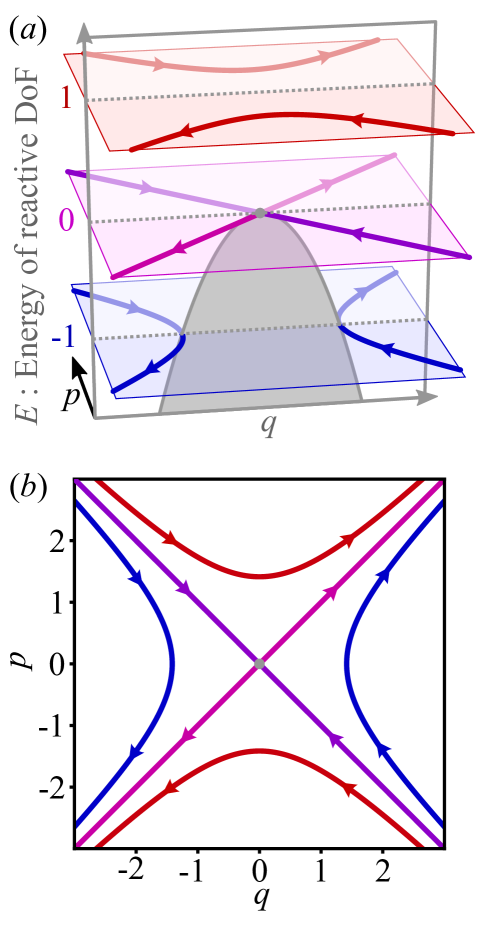
Figure 2: The phase space flow of trajectories along a reactive DoF is shown for various energies and its projection in phase space. For simplicity, the Hamiltonian, ${\cal H}=(p^{2}-q^{2})/2$, of this hyperbolic normal mode is taken to be that at second order in the potential expansion. Reactive trajectories (red, $E=1$), non-reactive trajectories (blue, $E=-1$), and trajectories on the reactivity boundary (purple and pink, $E=0$) in (a) the $q$-$p$-$E$ space, and (b) $q$-$p$ space. The potential energy surface is also drawn in gray on (a) $q$-$E$ plane.

For the normal mode approximation of a Hamiltonian expanded at an index-one saddle point:

$$H_{0}(\bm{p},\bm{q}) =\frac{1}{2}(p_{1}^{2}-\omega_{1}^{2}q_{1}^{2})+\frac{1}{2}\sum_{i=2}^{n}(p_{i}^{2}+\omega_{i}^{2}q_{i}^{2}),$$ (1)

here we use $i$th normal mode coordinate $q_{i}$, its conjugate momentum $p_{i}$, its frequency $\omega_{i}$, the coordinates vector $\bm{q}=(q_{1},\dots,q_{n})$, and the momenta vector $\bm{p}=(p_{1},\dots,p_{n})$. For all $i$, $\omega_{i}$ is positive so that $\omega_{1}\mathrm{i}$ is a pure imaginary frequency. The index of a potential energy saddle point is determined by the number of Hessian eigenvalues, which correspond to the Morse index of a critical point. The Hamiltonian equation of motion can be written with $(\bm{p},\bm{q})$ by

$$\derivative{t}\matrixquantity(p_{i}\\ q_{i})=\matrixquantity(\mp\omega_{i}^{2}q_{i}\\ p_{i}),$$ (2)

where $\mp$ correspond to the sign of the monomial $\pm\omega_{i}^{2}q_{i}^{2}$ in Eq. (1), respectively. The first normal mode $i=1$ is called hyperbolic or reactive DoF, and is shown in Fig. 2 with $\omega_{1}=1$. In the upper panel (2a), trajectories with given reactive mode-energies are shown relative to the corresponding potential energy saddle. When the mode-energy is positive and negative, the trajectory is reactive and non-reactive, respectively. The boundaries in between consist of asymptotic trajectories with zero mode-energy toward or from the origin. Here, the origin of the reactive DoF is called the NHIM, and its dimensionality grows as the total number of DoFs is increased. The trajectories asymptotic toward or from the NHIM are called the stable or unstable manifolds of the NHIM, respectively. In Wigner’s TST formulation,Wigner (1938) the dividing surface is defined as $q_{1}=0$ and $p_{1}>0$. Thus, the NHIM: $(p_{1},q_{1})=(0,0)$ is known as an anchor of the dividing surface. For a normal mode Hamiltonian, one can solve the equation of motion by the finding constants of motion, i.e., normal mode action $\bm{J}$. One can rewrite the reference Hamiltonian as

$$H_{0}=\sum_{i=1}^{n}\omega_{i}J_{i}(p_{i},q_{i}),$$ (3)

where the $i$th generalized momentum is

$$J_{i}=\begin{cases}\frac{1}{2\omega_{i}}(p_{i}^{2}-\omega_{i}^{2}q_{i}^{2})~{}(i=1)\\ \frac{1}{2\omega_{i}}(p_{i}^{2}+\omega_{i}^{2}q_{i}^{2})~{}(i\geq 2)\\ \end{cases}.$$ (4)

which is conjugate to the action $\theta_{i}$, and together satisfy

$$\derivative{t}\matrixquantity(J_{i}\\ \theta_{i})=\matrixquantity(-\partialderivative*{H_{0}}{\theta_{i}}\\ \partialderivative*{H_{0}}{J_{i}})=\matrixquantity(0\\ \omega_{i})$$ (5)

with its solution $\theta_{i}=\omega_{i}t,J_{i}=\mbox{constant}{.}$.

If $H_{0}$ is dominant, a similar relation can be obtained from CPT. When one can expand the Hamiltonian at the index-one saddle point:

$$H(\bm{p},\bm{q})=H_{0}(\bm{p},\bm{q})+\sum_{k=1}\epsilon^{k}{V}_{k}(\bm{q}),$$ (6)

where $V_{k}(\bm{q})$ is a ($k+2$)-order polynomial in $\bm{q}$, and the perturbation order $k$ is tracked by $\epsilon=1$ without changing the equation.

The construction of perturbation theory now follows a series of canonical transformations that successively remove the terms in $\theta$ up to a desired order while formally preserving the Hamiltonian structure. That is, we seek to find the composite transformation from $(\hat{\bm{p}},\hat{\bm{q}})$ to $(\hat{\bm{J}},\hat{\bm{\theta}})$ such that the new Hamiltonian is $H=\check{H}(\hat{\bm{J}})+\order{\epsilon^{k}}$. In Lie-CPT, this is achieved through a “time” propagation that go forward or backward in time resulting in the solutions, $\hat{F}$ and $\check{F}$, respectively. One can solve the equation of motion of $\check{H}$ with the order of accuracy $\order{\epsilon^{k}}$, i.e.,

$$\derivative{t}\matrixquantity(\hat{J}_{i}\\ \hat{\theta}_{i})=\matrixquantity(-\partialderivative*{\check{H}}{\hat{\theta}_{i}}\\ \partialderivative*{\check{H}}{\hat{J}_{i}})=\matrixquantity(0\\ \tilde{\omega}_{i}),$$ (7)

where $\tilde{\omega}_{i}:=\partialderivative*{\check{H}}{\hat{J}_{i}}$. This equation can be rewritten with $(\hat{\bm{p}},\hat{\bm{q}})$ as

$$\derivative{t}\matrixquantity(\hat{p}_{i}\\ \hat{q}_{i})=\frac{\tilde{\omega}_{i}(\hat{\bm{J}})}{\omega_{i}}\matrixquantity(\mp\omega_{i}^{2}\hat{q}_{i}\\ \hat{p}_{i}),$$ (8)

where the difference from Eq. (2) is the locally constant term, $\tilde{\omega}_{i}(\hat{\bm{J}})/\omega_{i}$. Therefore, the coordinate transformation $(\bm{p},\bm{q})\to(\hat{\bm{p}},\hat{\bm{q}})$ gives a local (in the sense of $\order{\epsilon^{k}}$) independence for each DoF including the reactive DoF $(i=1)$. This suggests that the phase space flow of Eq. (8) has a similar shape with Fig. 2, but in the space of $(\hat{\bm{p}},\hat{\bm{q}})$. Revisiting the flow of the trajectories without specifically constructing the Lie-CPT transformations should thus result in an alternate constrution revealing the reaction path, and serves to motivate the approach pursued here.

II.2 Inhomogeneity of the LD on the NHIM

Figure 3: Forward extremal Lagrangian Descriptor $\mathcal{L}^{\mathrm{f}}$ (arc length of a trajectory) over initial conditions of a 2-DoF harmonic system: $H=\sum_{i=1,2}p_{i}^{2}/(2m_{i})+m_{i}k_{i}q_{i}^{2}/2$ where $m_{1}=0.2,k_{1}=0.2,m_{2}=5,k_{2}=3$, with $E=10$, $q_{2}(0)=0$, and $p_{2}(0)>0$. The light-yellow area is energetically prohibited. (a) time evolution of $\mathcal{L}^{\mathrm{f}}(t)$ for $q_{1}(0)=0$ in $t-p_{1}(0)$ space, (b) $\mathcal{L}^{\mathrm{f}}(t=1000)$ in $q_{1}(0)-p_{1}(0)$ space.

To obtain the NHIM and its stable and unstable manifolds non-perturbatively, the LCS and LD are introduced here. In dynamical systems theory, a distinguished hyperbolic trajectory has been definedIde et al. (2002) as the non-autonomous analogue of a hyperbolic fixed point. Mancho and coworkersJiménez Madrid and Mancho (2009); Mendoza and Mancho (2010) introduced the form of the LD initially as a means to locate these distinguished hyperbolic trajectories.

Specifically in the context of the reaction dynamics, Craven and HernandezCraven and Hernandez (2015) implemented the extremal LD, $\mathcal{M}_{\mathrm{ex}}$, which describes the arc length of trajectories in coordinate space

$$\mathcal{M}_{\mathrm{ex}}(\bm{q}_{0},\dot{\bm{q}_{0}},t_{0};t):=\int_{t_{0}-t}^{t_{0}+t}\|\dot{\bm{q}}\|\differential t\;.$$ (9)

The arc length also evaluated for the forward and backward LDs:

$$\mathcal{L}_{\mathrm{f}} := \int_{t_{0}}^{t_{0}+\tau}\|\dot{\bm{q}}\|\differential t$$ (10a)

$$\mathcal{L}_{\mathrm{b}} := \int_{t_{0}-\tau}^{t_{0}}\|\dot{\bm{q}}\|\differential t$$ (10b)

to estimate stable and unstable manifolds, respectively, as the “abrupt change”Mancho et al. (2013) of LDs.

The LDs, $\mathcal{L}_{\mathrm{f}}$ and $\mathcal{L}_{\mathrm{b}}$, —refer to Eq. 10— are accumulated value of a positive scalar along a trajectory. Trajectories that diverge from each other will necessarily accumulate different LDs, and the separation of these values appear to signal the presence of a stable/unstable manifold of the NHIM that lies between them.Mancho et al. (2013) Although there are known examples that the singular contour of the LD correctly corresponds to the stable/unstable manifolds, there is no general proof on the correspondence. Formally, the LDs would be obtained at $t\to\infty$ where the values all go to infinity regardless of the choice of trajectory. The exceptions arise from fixed points at which the LD of trajectories asymptotic to them converges to a finite value. In practice, we integrate for a long, but finite, time at which there is a visible feature, deviation, or “abrupt change” in the LD between initially nearby trajectories, or abrupt features in the LD such as narrow ridges or valleys.

There are some concerns about the generality of the conjecture. In particular, HallerHaller (2016) criticized the use of the LD because it is not objective. That is, as long as the LD is defined by a norm, such as an arc length, the LD value is not necessarily independent of the particular choice of DoFs. To illustrate this concern, let us consider a three-dimensional normal mode Hamiltonian which has one reactive DoF and two vibrational DoFs. If the trajectory is on the NHIM, the dynamical variables $(q,p)$ of the reactive DoF remain constant, i.e., they remain on the saddle with zero reactive velocity. If LD values are uniform over the two vibrational DoFs, the reactive DoF is then the only relevant DoF. However, this is not the case as shown in Fig. 3. On the other hand, for the reactive mode $(q_{0},p_{0})$ of a normal mode Hamiltonian, a trajectory on the stable and unstable manifolds of the NHIM, with a momentum expressed by $p_{0}(0)\mathrm{e}^{-\lambda t}$ and $p_{0}(0)\mathrm{e}^{\lambda t}$, reaches the NHIM at $t\rightarrow\infty$ and $t\rightarrow-\infty$ respectively. This means that around the NHIM, extremal LD can be affected by the reactive DoF and be prone to dominant contributions from the vibrational DoFs. In some cases, modification of some initial conditions along the manifold can have larger effects on the LD value than from those not along the manifold. For these cases, the ‘abrupt’ change in the LD value could misidentify the region as containing NHIM NHIM. Thus the use of the LD to identify NHIMs has to be done with care.

II.3 Asymptotic Trajectory Indicator

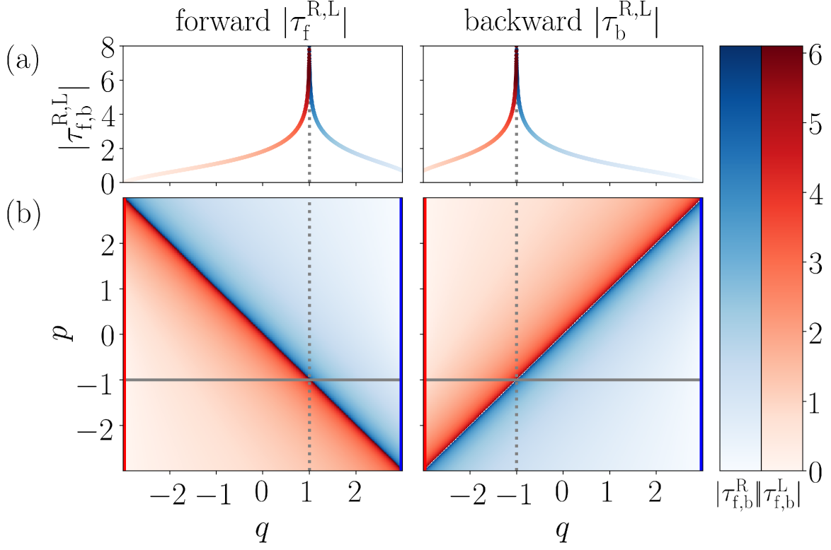
Figure 4: The forward ATI, $\tau_{\mathrm{f}}^{\mathrm{R,L}}$ (left column), and backward ATI, $\tau_{\mathrm{b}}^{\mathrm{R,L}}$ (right column), defined in Eqs. (16) and (17) respectively. They correspond respectively to the first hitting time of the right $q=3$ (blue) and left $q=-3$ (red) absorbing boundary starting from the given point. Panel (a) shows the values along the gray line plotted in phase space (b). The dashed line corresponds to the singular point along the gray line in (b). The Hamiltonian is the same as in Fig. 2.

An alternative to the LD can be achieved through the reactivity bands (in one-dimensional domains) or reactivity map (in higher dimension)Wall et al. (1958, 1961); Wall and Porter (1963); Wright et al. (1975, 1976); Wright and Tan (1977); Wright (1978); Laidler et al. (1977); Tan et al. (1977) and reactivity boundary.Nagahata et al. (2013a) These structures are defined on the domain of initial condition in phase space by designating them according to their ultimate origin or destination to a reactant domain or one of possibly many distinct product domains. Between initial conditions assigned to different final basins, there could be initial conditions whose trajectories never reach one of the designated basins, and thus act as reactivity boundary.Nagahata et al. (2013a) For example, the purple and pink trajectories in Fig. 2 form the boundary between initial conditions assigned to products (at $t\to+\infty$) and reactants (at $t\to-\infty$), respectively. Together, these boundaries separate trajectories into four categories whose initial and final chemical state can be assigned according to whether trajectories are (1) staying inside of, (2) entering into, (3) exiting from, or (4) staying outside of the trapping area. Those structures are fundamental to the turnstileMackay et al. (1984) and reaction islandOzorio de Almeida et al. (1990) theories.

To compare with the NHIM theory,Fenichel (1972); Wiggins (1994); Eldering (2013) let us formulate the reactivity boundaries mathematically by using their asymptotic nature. Let $\bm{\phi}^{t}$ be the propagator in time $t$, i.e., a flow function,

$$\bm{\phi}^{t}:\bm{x}(t_{0})\rightarrow\bm{x}(t_{0}+t).$$ (11)

For given $\bm{\phi}^{t}$, there could be a set of trajectories, which is restricted to a subspace $\mathcal{M}$. Such a subspace $\mathcal{M}$ of the phase space $\mathcal{P}$ is said to be invariant when

$$\mathcal{M}:=\left\{\bm{x}\middle|\forall\bm{x}\in\mathcal{M}~{}\mathrm{and}~{}\forall t,\bm{\phi}^{t}(\bm{x})\in\mathcal{M}\right\}.$$ (12)

Or more simply, $\mathcal{M}$ is an invariant subspace when $\bm{\phi}^{t}(\mathcal{M})=\mathcal{M}$ for arbitrary $t$. If there are asymptotic trajectories to $\mathcal{M}$ then one can define the stable manifold and unstable manifold of the invariant manifold $\mathcal{M}$ as follows:

$$\mathcal{W}_{\mathcal{M}}^{\mathrm{(s)}}:= \left\{\bm{x}\middle|\forall\bm{x}\in\mathcal{P},\lim_{t\rightarrow\infty}\bm{\phi}^{t}(\bm{x})\in\mathcal{M}\right\},$$ (13)

$$\mathcal{W}_{\mathcal{M}}^{\mathrm{(u)}}:= \left\{\bm{x}\middle|\forall\bm{x}\in\mathcal{P},\lim_{t\rightarrow-\infty}\bm{\phi}^{t}(\bm{x})\in\mathcal{M}\right\}.$$ (14)

Accordingly, $\mathcal{W}_{\mathcal{M}}^{\mathrm{(s)}}\cap\mathcal{W}_{\mathcal{M}}^{\mathrm{(u)}}$ is invariant. For simplicity, we define the reactivity boundary separating the destination and origin of trajectories as $\mathcal{W}_{\mathrm{asym}}^{\mathrm{(s)}}$ and $\mathcal{W}_{\mathrm{asym}}^{\mathrm{(u)}}$ respectively. This allows us to designate an invariant manifold related only to $\mathcal{W}_{\mathrm{asym}}^{\mathrm{(s)}}$ and $\mathcal{W}_{\mathrm{asym}}^{\mathrm{(u)}}$ as

$$\mathcal{M}_{\mathrm{asym}}:=\mathcal{W}_{\mathrm{asym}}^{\mathrm{(s)}}\cap\mathcal{W}_{\mathrm{asym}}^{\mathrm{(u)}},$$ (15)

where $\mathcal{W}_{X}^{\mathrm{(s)}}:=\mathcal{W}_{\mathcal{M}_{X}}^{\mathrm{(s)}}$, and $\mathcal{W}_{X}^{\mathrm{(u)}}:=\mathcal{W}_{\mathcal{M}_{X}}^{\mathrm{(u)}}$ for $X=\mathrm{asym}$.

In practice, this manifold $\mathcal{M}_{\mathrm{asym}}$ can be detected through observation of nearby trajectories. We first identify a subspace $\mathcal{S}$ that contains $\mathcal{M}_{\mathrm{asym}}$ —i.e., $\mathcal{S}$ $\supset\mathcal{M}_{\mathrm{asym}}$,— with initial conditions associated with trajectories that remain in $\mathcal{W}_{\mathrm{asym}}^{\mathrm{(s)}}$ under forward propagation or $\mathcal{W}_{\mathrm{asym}}^{\mathrm{(u)}}$ under backward propagation. We then define the first passage time for each point $x\in\mathcal{S}$ according to when it first crosses the boundary $\partial\mathcal{S}$, that is,

$$\tau_{\mathrm{f}}(\bm{x};\mathcal{S}):=\min_{t}\left\{t\middle|\forall t\geq 0,\bm{\phi}^{t}(\bm{x})\in\partial\mathcal{S}\right\}.$$ (16)

Consequently, for $\bm{x}\in\mathcal{W}_{\mathrm{asym}}^{\mathrm{(s)}}$, then $\tau_{\mathrm{f}}(\bm{x};\mathcal{S})=\infty$. Neighbors $\bm{y}$ of $\bm{x}\in\mathcal{W}_{\mathrm{asym}}^{\mathrm{(s)}}$, will necessarily have large but finite $\tau_{\mathrm{f}}(\bm{y};\mathcal{S})$ because of the continuity of the equation of motion. Therefore, abrupt changes in $\tau_{\mathrm{f}}(\bm{x};\mathcal{S})$ indicate the nearby location of the singular contour, i.e., $\mathcal{W}_{\mathrm{sing}}^{\mathrm{f}}:=\left\{\bm{x}\middle|\tau_{\mathrm{f}}(\bm{x};\mathcal{S})=\infty\right\}$. This contour is formed from forward asymptotic trajectories, and is therefore the manifold $\mathcal{W}_{\mathrm{asym}}^{(s)}$. For this reason, hereafter we call $\tau_{\mathrm{f}}(\bm{x};\mathcal{S})$ the forward asymptotic trajectory indicator (ATI). Similarly, we can define

$$\tau_{\mathrm{b}}(\bm{x};\mathcal{S}):=\max_{t}\left\{t\middle|\forall t\leq 0,\bm{\phi}^{t}(\bm{x})\in\partial\mathcal{S}\right\}$$ (17)

as the backward ATI. We provide an example in Fig. 4 to show a typical behavior of the ATI.

It is useful to consider how the ATI generalizes for more complex cases, including those when $\partial S$ encloses multiple asymptotic manifolds. In the following, we prove that when one observes an ATI value of a point on $\partial S$, its value is almost surely finite, if $S$ is compact. Here, “almost surely” means that the statement is true except for one or more dimensions less than an equi-energy surface of the phase space. First, let us consider a subset of initial conditions on $\partial S$, for which entire trajectories are not bounded to the region $S$. Each such trajectory must have an even number of intersections on $\partial S$ —that is, they go in and out in pairs— because it is not bounded. Second, the other initial conditions are known to be almost surely recurrent as specified by Poincaré’s recurrence theorem. (See, e.g., Sec. 3 16 D in Ref. Arnol’d, 1989.) Asymptotic trajectories serves as examples of such measure zero sets. Therefore, when one observes an ATI value of a point on $\partial S$, its value is almost surely finite, if $S$ is compact. In fact, below we observe the reactivity boundaries as singular contours even if $S$ includes multiple asymptotic manifolds. In practice, the finiteness of the ATI may indicate the requirement of very long time propagation. For example, a trajectory may be trapped in a potential energy well. The complexity of highly coupled reactions also challenges our approach because they can lead to fractal structures arising from chaotic dynamics. Such cases can be avoided by taking $S$ around a $\mathcal{M}_{\mathrm{asym}}$. In Subsec. IV.2, we further show heuristics to avoid long-time trajectory calculations.

II.4 Comparison with NHIM theory

Here we confirm that the ATI leads to NHIM NHIM in cases when the solution is accessible to perturbation theory, and how it extends beyond it. To this end, we first observe that the NHIM Persistence Theorem provides for the persistence of the phase space geometry —vis-à-vis the NHIM— under perturbation. As we reconfirm in the Appendix A, the reaction dynamics around an index-one saddle on a potential energy surface satisfies the requisite conditions of the theorem. In this case, the NHIM corresponds to a DoFs orthogonal to the reactive DoF at the TS. The latter is the nonlinear analogue of the DoF associated with the eigenvector of the positive Hessian eigenvalue.

The stable and unstable manifolds associated to the reaction coordinate are illustrated in Fig. 2. They are associated with imaginary frequencies, called characteristic exponents throughout this work, that characterize their strongest decay. That is, the persistence of the manifolds results from their exponential expansion and contraction, respectively, and the sign of the characteristic exponent reflects this. Suppose for its imaginary frequency $\lambda_{\mathrm{s,u}}$ and upper bound of the other imaginary part of frequencies $\lambda_{\mathrm{c}}$, the NHIM has $r\geq 1$ such that, $0\leq r\lambda_{\mathrm{c}}<\lambda_{\mathrm{s,u}}$ (e.g. $\lambda_{\mathrm{c}}=0$ when the saddle is index one). In this case and if the flow is $k$-differentiable $\bm{\phi}^{t}\in C^{k}$, then $\mathcal{M}_{\mathrm{NHIM}}\in C^{k}$ when $k\leq r$. In addition, for a $f\in C^{k}$, $f(\mathcal{M}_{\mathrm{NHIM}})$ is still NHIM NHIM and $k$-differentiable, i.e., persistent under $C^{k}$ perturbation. Specifically, this NHIM is called a $k$-NHIM.Hirsch et al. (1977); Wiggins (1994); Eldering (2013) (See Appendix A for the explicit definition).

For example, if $\mathcal{M}(\subset\mathcal{S})$ is NHIM NHIM associated with an index-one saddle, the characteristic exponents $-\lambda_{\mathrm{s,u}}$ and $\lambda_{\mathrm{s,u}}$ corresponding to expansion and contraction directions are associated with stable $\mathcal{W}_{\mathrm{NHIM}}^{\mathrm{(s)}}$ and unstable $\mathcal{W}_{\mathrm{NHIM}}^{\mathrm{(u)}}$ manifolds, respectively. The singular contour of the ATIs defined in the previous section is a stable (i.e., $\mathcal{W}_{\mathrm{sing}}^{\mathrm{f}}$) or unstable (i.e., $\mathcal{W}_{\mathrm{sing}}^{\mathrm{b}}$) manifold of the NHIM.

More generally, $\mathcal{M}_{\mathrm{NHIM}}$ and $\mathcal{M}_{\mathrm{asym}}$ are not equivalent for higher index saddles. For example, if there are other exponentially growing directions with characteristic exponents $-\mu_{\mathrm{s}}$ and $\mu_{\mathrm{u}}$ in addition to those of that stable $-\lambda_{\mathrm{s}}$ and unstable $\lambda_{\mathrm{u}}$ manifolds, satisfying $-\lambda_{\mathrm{s}}<-\mu_{\mathrm{s}}<0<\mu_{\mathrm{u}}<\lambda_{\mathrm{u}}$, then the directions are tangent to $\mathcal{M}_{\mathrm{NHIM}}$ because of $\lambda_{\mathrm{c}}\geq\max\{\mu_{\mathrm{s}},\mu_{\mathrm{u}}\}$. On the other hand, those directions are still normal to $\mathcal{M}_{\mathrm{asym}}$ because they converge to it asymptotically. Therefore, $\mathcal{M}_{\mathrm{asym}}$ is not NHIM NHIM, and $\mathcal{M}_{\mathrm{asym}}$ may not have persistence under perturbation. Such a failure was recently seen for an index-2 saddle despite the convergence of perturbation theory.Nagahata et al. (2013b)

The reactivity boundary ($\mathcal{W}_{\mathrm{asym}}^{(x)}$ with $x=\mathrm{s,u}$) is relevant to reaction dynamics because it marks the transition at which the fate of the reactants is cast. For example, for a reaction with an index-1 saddle, the reactivity boundaries are the same as the stable and unstable manifolds of the NHIM. This feature allows us to detect the boundary of reactivity even for reactions associated with higher index saddles.Nagahata et al. (2013a)

II.5 NHIM of Random Dynamical Systems

The nature of a trajectory resulting from SDE stochastic differential equation (SDE) is completely different from an ordinary differential equation (ODE).Øksendal (2003); Duan (2015) For example, a particle whose motion is described by a Langevin equation is thereby driven stochastically by a random force $\xi(t)$ only in a formal sense. In practice, one must integrate over the latter to propagate the particle within a difference equation, e.g., by the Euler-Maruyama method.Kloeden and Platen (1992) Integrals of the random force are neither smooth nor continuous in the usual sense. Its statistics generally satisfy that of a Wiener process.Duan (2015) Specifically, we can define the difference in the accumulated random force across a time interval as

$$B_{s+t}-B_{s}\equiv\int_{s}^{s+t}\xi(\tau)\differential\tau\sim\mathcal{N}(0,Dt),$$ (18)

where $D$ is the diffusion constant. The relation $X\sim\mathcal{N}(\mu,\sigma^{2})$ is defined such that $X$ is a random variable resulting from a normal distribution with mean $\mu$ and variance $\sigma^{2}$. With this construction, $B_{t}$ has continuity in a weak sense; that is, it satisfies the $\beta$-Hölder continuity for all $\beta$ satisfying $\beta<1/2$.Øksendal (2003) Recall that $\beta$-Hölder continuity requires the existence of a constant $c>0$ and an exponent $\beta>0$ such that

$$|B_{t}-B_{s}|\leq c|t-s|^{\beta}.$$ (19)

for all times $t$ and $s$. We further require $\beta=1$ so that the function is differentiable. In the present case, the existence of weak continuity allows us to claim uniqueness of the solution for a given stochastic sequence, and hence each solution has pathwise uniqueness.Øksendal (2003) Second, as a consequence of the lack of smoothness in $B_{t}$, it is nowhere differentiable along $t$, and it can not be inverted to a $\xi$.

The NHIM Persistence Theorem describing the geometry of the solutions of the SDE can be framed through an analysis of the paths (trajectories) of the SDE. For each $d$-dimensional accumulated random force $\bm{B}_{t}$, one can uniquely obtain a $d$-dimensional, $t$-continuous function $\bm{\omega}(t)$ that is associated with the saddle point (precisely defined in Appendix C) at each instance of time $t$, and for which we are free to initialize at $\bm{\omega}(0)=0$. (Note that this $\bm{\omega}(t)$ is simply an abstraction of the so-called TS trajectory.Bartsch et al. (2005)) Then a probability is determined from a bundle of instances $\bm{\omega}$. Let us also introduce a $t$-origin shift to the probability measure, the so-called Wiener shift $\theta_{s}$, such that,

$$(\theta_{s}\bm{\omega})(t)=\bm{\omega}(s+t)-\bm{\omega}(s),~{}s>0.$$ (20)

This $\theta_{s}$ introduces a shift in the initial time of a stochastic process to $s$. For example, any given Brownian motion can be written as a particular manifestation of $\bm{\omega}$, such that, for $\bm{B}_{t}=\bm{B}[\bm{\omega}(t)]$,

$$\bm{B}[(\theta_{s}\bm{\omega})(t)]= \bm{B}[\bm{\omega}(s+t)-\bm{\omega}(s)]$$

$$= \bm{B}[\bm{\omega}(t+s)]-\bm{B}[\bm{\omega}(s)].$$ (21)

The relation can be found in Eq. (6.46) of Ref. Duan, 2015. (See also Eq. (18) for SDE SDE.) We can then define stochastic analogues of the flow function and invariant manifold associated with an ODE to the analogues of the SDE SDE: the stochastic cocycle $\bm{\phi}^{t}_{\bm{\omega}}$,

$$\bm{\phi^{t}_{\bm{\omega}}}:\bm{x}(s)\rightarrow\bm{x}(t+s;\theta_{s}\bm{\omega},\bm{x}(s)),$$ (22)

and the random invariant manifold $\mathcal{M}(\bm{\omega})$,

$$\bm{\phi}^{t}_{\bm{\omega}}(\mathcal{M}(\bm{\omega}))=\mathcal{M}(\theta_{t}\bm{\omega}),$$ (23)

respectively. In Eq. (22), the stochastic path $\bm{x}(\cdot)$ starts at $s$ requiring a shift in the time origin of $\bm{\omega}(t)$ to $s$, and hence the need for the term $\theta_{s}\bm{\omega}$ in the argument of $x$. RDS random dynamical system (RDS) defined by Eq. (22) is uniquely obtained from a random differential equation (RDE) with the vector field $\bm{f}$

$$\dot{\bm{x}}=\bm{f}(\theta_{t}\bm{\omega},\bm{x}),$$ (24)

as usually obtained for ODE. One can obtain this RDS for some classes of SDEs, including Langevin type equations. (See Appendix C.)

The NHIM Persistence Theorem for a RDS holdsLi et al. (2013) for random invariant manifolds defined by Eq. (23). The remarkable result of the theorem is that the NHIM is persistent under $C^{1}$ perturbations and is $C^{k}$-smooth at time $t$ when $\bm{\phi}^{t}_{\bm{\omega}}\in C^{k}$. The smoothness of $\bm{\phi}^{t}_{\bm{\omega}}$ does not indicate that the variables of SDE —e.g. of the Langevin equation— are smooth over integration time. On the other hand, SDE still has a Hölder continuity as detailed above. Because of this continuity, the closer an initial condition is to the stable or unstable manifold of NHIM NHIM, then the longer the trajectory will spend in time around the NHIM. In this way, there can still exist abrupt changes and singular contours in the ATIs of SDE SDE, where the latter corresponds to the NHIM and its stable and unstable manifolds. Because of the theorem, these manifolds are smooth.

As was suggested in Refs. Li et al., 2013; Eldering, 2013, the NHIM Persistence Theorem holds for autonomous systems. For such systems, there is a single $\bm{\omega}$ which corresponds to the time series of the external forceArnold (2003) and does not require any fundamental change to satisfy the conditions needed to satisfy the NHIM Persistence Theorem.Eldering (2013)

III Neighbor Bisection and Continuation with ATI

Thus far, we have considered the case of a single invariant manifold $\mathcal{M}_{\mathrm{asym}}$ defined in Eq. (15) that lives within the subspace $\mathcal{S}$ of the phase space $\mathcal{P}$ without considering the computational requirements for its implementation. In practice, the latter is exacerbated by the existence of multiple NHIMs in $\mathcal{S}$. Nevertheless, typically some features of its structure (such as possible location or locations) are approximately known, and they can be used to optimize sampling of candidate points of the manifold, and improve the numerical implementation of the search. Here, we present a practical approach for defining the absorbing boundaries, sampling the surrounding neighborhood of the reactivity boundary, and visualizing the ATI. We introduce the NBC-ATI method to effectively increase the resolution and accuracy of the reactivity boundaries.

III.1 Absorption and Visualization

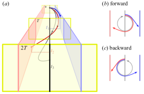
Figure 5: A schema of possible trajectories from an initial point in the region relative to the absorbing boundary surfaces is shown in panel (a) as a function of time: A trajectory hitting the left (in red) or right (in blue) absorbing boundary, and a recurrent trajectory (in gray) which returns to the same coordinate with the same sign in the velocity. The projection of these trajectories in forward and backward time onto the phase space is shown in panels (b) and (c), respectively.

The values of the forward $\tau_{\mathrm{f}}$ and backward $\tau_{\mathrm{b}}$ times defined in Sec. II depend on the initial and absorbing conditions. However, the location of the singular contour in $\tau$ corresponding to the reactivity boundary is independent of the absorbing conditions, as we described in Sec. II.3. A naive absorbing condition can be defined through a coordinate $\bm{q}$ at a value that is significant to the dynamics (e.g., at a potential energy minimum) and sufficiently far away from the TS. Figure 5 illustrates an example in which trajectories are absorbed and thereafter assigned a first hitting time $\tau$ —viz, the ATI.

The domain of initial conditions can be labeled using a color that denotes one of the surfaces shown in Fig. 5 to which they absorb, and an intensity commensurate with the value of the ATI, $\tau$. The result for a normal mode Hamiltonian is illustrated in Fig. 4. Initial conditions on the domain are labeled in red or blue according to whether trajectories are absorbed on the left at $q=-3$ or right at $q=3$, respectively. The intensity of the color is commensurate with the value of the ATI, $\tau_{\mathrm{f}}^{\mathrm{L}}$ or $\tau_{\mathrm{f}}^{\mathrm{R}}$. In the context of the theory described in Sec. II, the absorbing boundaries at $\mathrm{R}$ and $\mathrm{L}$ employed here are examples of the two disconnected subsets of $\partial\mathcal{S}$.

As shown in Fig. 4a, $\tau_{\mathrm{f}}$ or $\tau_{\mathrm{b}}$ has a singular contour for the forward or backward asymptotic trajectories that corresponds to the purple or pink trajectories in Fig. 2, respectively. Hence, the abrupt change in $\tau_{\mathrm{f}}$ or $\tau_{\mathrm{b}}$ in Fig. 4b indicates that there is, indeed, a reactivity boundary nearby. This singular contour is the stable or unstable manifold of the NHIM. For the present case, the NHIM is $(q,p)=(0,0)$, the stable manifold is $p=-q$, and the unstable manifold is $p=+q$.

III.2 Efficient Sampling Algorithm

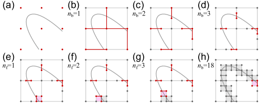
Figure 6: Schema of selected steps in the sampling algorithm as described in the text. In any given step, the active straddling pairs (red), points (red) and area (magenta), are highlighted in color, and previously sampled straddling pairs (gray), area (light gray) and point (gray) are highlighted in gray scale.

When analytical methods, such as perturbation theory, fail to produce the exact form of the reactivity boundary, we must resort to using numerical methods. The challenge to the numerics, however, lies in the fact that the reactivity boundary has measure zero, and hence statistical sampling is inefficient. To overcome this challenge, we employ an algorithm which effectively generalizes the one-dimensional bisection method to 2D and the required higher dimensionality of the space that contains the reactivity boundary. It may be implemented iteratively when a user needs to improve resolution to, for example, increase the number of points of the reactivity boundary.

To initiate the first stage of the algorithm, we need a low-resolution representation of the reactivity boundary. We can construct this by way of creating a low-resolution grid in the domain, and performing a “brute-force search” across all the vertices to identify pairs of points that straddle the reactivity boundary in the sense that one of the two adjacent points goes to the reactant-side surface and the other to the product-side surface. We call such pairs of points straddling pairs. In more detail, we execute the brute-force search on a $(2^{N_{\mathrm{BF}}}+1)\times(2^{N_{\mathrm{BF}}}+1)$ grid ($N_{\mathrm{BF}}=1$ in Fig. 6a). The grid results in a spacing resolution at $\bm{L}/2^{N_{\mathrm{BF}}}$ where for the length of given 2D rectangle domain $\bm{L}=(L_{x},L_{y})$. As long as the reactivity boundary does not fold within a width of this resolution, a straddling pair will capture one of its points within its connecting segment.

In the first stage — “seed refinement” —, we refine the initial straddling pairs up to the desired resolution. Specifically, we iterate the bisection method $N_{\mathrm{res}}-N_{\mathrm{BF}}$ times to find a new set of straddling pairs to the desired grid resolution, i.e., $(2^{N_{\mathrm{res}}}+1)\times(2^{N_{\mathrm{res}}}+1)$. In this stage, we assume that the desired structures are all larger than the resolution of the initial grid. The resulting resolution of the straddling pairs, illustrated in Fig. 6b-d for $N_{\mathrm{res}}=3$, is on the order of $\bm{L}/2^{N_{\mathrm{res}}}$.

In the second stage — “path-following” or “continuation” —, we construct edge-to-edge and recurrent chains of straddling pairs. To construct edge-to-edge chains, we first choose one of straddling pairs which are on the edge of the domain. If it exists, then we use the pair to identify a next pair (red line in Fig. 6e-h) that also straddles the reactivity boundary. A chain of straddling pairs is constructed by repeating this iteration until it reaches the edge of the domain (Fig. 6h). If after this construction, there remains straddling points on the edge, we pick one of them and apply the path-following stage above until they are exhausted. To construct recurrent chains, we then repeat the procedure on remaining straddling pairs inside the domain, which will necessarily end on themselves, until all straddling pairs are exhausted.

In the third stage — “precision refinement” —, we refine the precision of the straddling pairs of the obtained chains. We apply the bisection method to each identified straddling pair $N_{\mathrm{pre}}-N_{\mathrm{res}}$ times to achieve the desired grid precision $(2^{N_{\mathrm{pre}}}+1)\times(2^{N_{\mathrm{pre}}}+1)$ with $\bm{L}/2^{N_{\mathrm{pre}}}$. In the numerical applications, we chose $N_{\mathrm{pre}}=30$. Because $2^{-30}\approx 10^{-9}$ and the highest resolution in double-precision is 16 decimal digits, then the points between straddling pairs can be differentiated only up to $7$ additional digits. If we use ${10}^{-13}$ for the desired accuracy in the time integration, then we still have $4$ reliable such digits in a single iteration of time propagation. Thus, for this setup, the computational result is reliable as long as the accumulated numerical error through the time propagation for obtaining $\tau$ is less than a factor of $10^{4}$ times the error of a single step iteration.

Table 1: Number of evaluated trajectories in each stage of the sampling algorithm. $C_{\mathrm{st}}[resolution;\mathcal{M}]$ and $C_{\mathrm{sq}}[resolution;\mathcal{M}]$ are the number from straddling pairs and that from covering squares of $\mathcal{M}$ in the given $resolution$, respectively.

Stage	Method	Number of evaluated trajectories
		Exact	Order (expected)
0th	Brute-Force	${(2^{N_{\mathrm{BF}}}+1)}^{2}$	$2^{2N_{\mathrm{BF}}}$
1st	Bisections	$C_{\mathrm{st}}{[2^{N_{\mathrm{BF}}}+1;\mathcal{M}]}\times(N_{\mathrm{res}}-N_{\mathrm{BF}})$	$2^{N_{\mathrm{BF}}}\times(N_{\mathrm{res}}-N_{\mathrm{BF}})$
2nd	Path-Following	$C_{\mathrm{sq}}{[2^{N_{\mathrm{res}}}+1;\mathcal{M}]}-C_{\mathrm{st}}{[2^{N_{\mathrm{BF}}}+1;\mathcal{M}]}$	$2^{N_{\mathrm{res}}}$
3rd	Bisections	$C_{\mathrm{st}}{[2^{N_{\mathrm{res}}}+1;\mathcal{M}]}\times(N_{\mathrm{pre}}-N_{\mathrm{res}})$	$2^{N_{\mathrm{res}}}\times(N_{\mathrm{pre}}-N_{\mathrm{res}})$

Suppose that we use a $(2^{N_{\mathrm{BF}}}+1)\times(2^{N_{\mathrm{BF}}}+1)$ grid in defining our initial search space, and we wanted to get a resolution of $\delta\bm{L}/2^{N_{\mathrm{res}}}$. Naively, this would require the determination of ${(2^{N_{\mathrm{res}}}+1)}^{2}$ points on a two-dimensional grid. Using our algorithm, instead, we expect that the number of points is approximately proportional to $2^{N_{\mathrm{res}}}$. This estimate is based on an assumption that the number of straddling pairs on a $(2^{N_{\mathrm{res}}}+1)\times(2^{N_{\mathrm{res}}}+1)$ grid $C_{\mathrm{st}}{[2^{N_{\mathrm{res}}}+1;\mathcal{M}]}$ is proportional to $2^{N_{\mathrm{res}}}$, where $\mathcal{M}$ is the manifold whose straddling pairs we are identifying. The assumption is trivially correct when $\mathcal{M}$ is one-dimensional on the observed two-dimensional domain. In that case, the order estimation can be made with the relation: $C_{\mathrm{st}}[x;\mathcal{M}]\leq C_{\mathrm{sq}}[x;\mathcal{M}]\leq(9/5)C_{\mathrm{st}}[x;\mathcal{M}]$, where $C_{\mathrm{sq}}$ is the number of points attach to the squares with resolution $x$ covering $\mathcal{M}$, and the first and the second equality are from the cases when all the straddling pairs have a different and the same orientation from that of the adjacent pair, respectively. We know that the $N$-fold application of the bisection method to a straddling pair needs the calculation on $N$ additional points, and the number of input seeds for the path-following stage is $C_{\mathrm{st}}{[2^{N_{\mathrm{BF}}}+1;\mathcal{M}]}$. We listed the order of magnitude for the number of points for each stage in Table 1. Based on this table, if we chose $2^{N_{\mathrm{BF}}}\ll 2^{N_{\mathrm{res}}}$, then the order can be estimated as $2^{N_{\mathrm{res}}}$. When we include the third stage in the estimation, the order becomes $N_{\mathrm{pre}}-N_{\mathrm{res}}+1$ times larger than the order up to the second step.

For $n$ DoF systems at a constrained energy, the number of 2D slices required to visualize the entire reactivity boundary in phase space becomes $N^{(2n-1)-2}>1(n\geq 2)$, where $N$ is the number of points sampled along a given axis. Thus, a naive estimation of the computational cost is on the order of ${(2^{N_{\mathrm{res}}})}^{(2n-1)-1}$ if the cost of each slice is same as above: $2^{N_{\mathrm{res}}}$ and $N=2^{N_{\mathrm{res}}}$. Not coincidentally, this exponent (=$(2n-1)-1$) is the same as the dimension of the reactivity boundaries, i.e., $\mathcal{W}_{\mathrm{asym}}^{\mathrm{(s)}}$ and $\mathcal{W}_{\mathrm{asym}}^{\mathrm{(u)}}$. In Fig. D.3 of Appendix D, we illustrate how the order estimates surmised here correspond to the computational cost seen in practice.

The output of the algorithm —i.e., the chain of straddling pairs— can be used to sample other parts of the boundary by propagating forward or backward in time (See Fig. D.4 for example). However, due to the nature of a trajectory on a stable or unstable manifold, the distance between adjacent straddling pairs will exponentially increase by the propagation. Thus, depending on the integration time, we may need to obtain more pairs in between some pairs we already have. In such cases, we can use the output as an input to the first stage of the algorithm. We can then apply the bisection method $N_{\mathrm{res}}^{\prime}$ times father, and thereby obtain $2^{N_{\mathrm{res}}^{\prime}}$ times greater resolution than the input as the output. The interactive application of our algorithm thus results in an approximate curve representing the reactive boundary to a desired resolution (by the second stage) and precision (by the third stage.)

IV NBC-ATI Analysis of Ketene Isomerization

IV.1 Reduced Ketene Model

Table 2: Parameters of the reduced ketene model of Eq. (25) taken from Ref. Gezelter and Miller, 1995.

Parameter	Value	Unit
$a_{2}$	$-2.3597\times 10^{-3}$	$E_{\mathrm{h}}a_{0}^{-2}$
$a_{4}$	$1.0408\times 10^{-3}$	$E_{\mathrm{h}}a_{0}^{-4}$
$a_{6}$	$-7.5496\times 10^{-5}$	$E_{\mathrm{h}}a_{0}^{-6}$
$c$	$7.7569\times 10^{-3}$	$E_{\mathrm{h}}a_{0}^{-2}$
$d$	$1.9769$	$a_{0}^{-2}$
$m_{\mathrm{F}}$	$9580.46$	$m_{\mathrm{e}}$
$m_{\mathrm{H}}$	$1837.1$	$m_{\mathrm{e}}$
$k_{1}$	$1.0074\times 10^{-2}$	$E_{\mathrm{h}}a_{0}^{-2}$
$d_{1}$	$-2.45182\times 10^{-4}$	$E_{\mathrm{h}}a_{0}^{-5}$
$k_{2}$	$2.9044\times 10^{-2}$	$E_{\mathrm{h}}a_{0}^{-2}$
$d_{2}$	$-8.5436\times 10^{-4}$	$E_{\mathrm{h}}a_{0}^{-5}$

To illustrate the NBC-ATI method, we apply it to the reaction dynamics of ketene to uncover its reaction geometry by ATIs. To this end, we use a reduced model of ketene introduced by Gezelter and MillerGezelter and Miller (1995) and adopted by Craven and Hernandez to illustrate LDs.Craven and Hernandez (2016)

$$V(q_{\mathrm{F}},q_{1},q_{2}):=V_{\mathrm{F}}(q_{\mathrm{F}})+\sum_{i=1,2}\frac{k_{i}}{2}{\left(q_{i}+d_{i}\frac{q_{\mathrm{F}}^{4}}{k_{i}}\right)}^{2},$$ (25a)

$$V_{\mathrm{F}}(q_{\mathrm{F}}):=a_{2}q_{\mathrm{F}}^{2}+a_{4}q_{\mathrm{F}}^{4}+a_{6}q_{\mathrm{F}}^{6}+cq_{\mathrm{F}}^{2}\mathrm{e}^{-dq_{\mathrm{F}}^{2}}.$$ (25b)

We use the parameters fitted by Gezelter and MullerGezelter and Miller (1995) reproduced in Table 2 with the correction on $m_{\mathrm{F}}$ by Ulusoy et al.Ulusoy and Hernandez (2014) The fit is based on the result of an ab initio calculation at the level of CCSD(T)/6–311G(df,p) by Scott et al.,Scott et al. (1994) where $q_{\mathrm{F}}$, $q_{1}$ and $q_{2}$ are coordinates of the systems. This model uses the normal mode coordinate of the oxirene geometry.Gezelter and Miller (1995) That is, $q_{\mathrm{F}}$ is the motion along the normal mode reaction coordinate, $q_{1}$ is the out-of-plane wagging and twisting motion of the hydrogens relative to CCO plane, and $q_{2}$ is the in-plane rocking and scissoring motion of the hydrogens relative to CCO plane. All the parameters are fixed to reproduce the structures of oxirene and formylmethylene intermediates.

Ketene is known for its remarkable photo-isomerization and photo-dissociation behavior as first observed by Moore et al.Lovejoy et al. (1991, 1992); Lovejoy and Moore (1993) Its unusual reaction dynamics was discussed in the context of roaming reactions withoutUlusoy et al. (2013); Ulusoy and Hernandez (2014); Mauguière et al. (2017) and withCraven and Hernandez (2016) the application of external forces. In the latter case, the interaction drives a dipole along $q_{\mathrm{F}}$ whose moment was obtained using B3LYP/6–311+G** by Craven and Hernandez.Craven and Hernandez (2016) The resulting potential interaction, and dipole moment can be written as

$$V_{\mathrm{ex}}(q_{\mathrm{F}},t)= \mathcal{E}_{0}\sin(\omega t)\mu_{m}(q_{\mathrm{F}})$$ (26a)

$$\mu_{m}(q_{\mathrm{F}}):= \mu_{0}(\mathrm{e}^{-\alpha{(q_{\mathrm{F}}-q_{0})}^{4}}+\mathrm{e}^{-\alpha{(q_{\mathrm{F}}+q_{0})}^{4}})$$

$$+\mu_{\mathrm{ketene}}$$ (26b)

with the parameters reproduced in Table 3.

Table 3: Parameters of the external force of Eq. (26) taken from Ref. Craven and Hernandez, 2016

Parameter	Value	Unit
$\mu_{0}$	$0.546$	$ea_{0}$
$\mu_{\mathrm{ketene}}$	$0.602$	$ea_{0}$
$q_{0}$	$1.95$	$a_{0}$
$\alpha$	$0.0701$	$a_{0}^{-4}$
$\mathcal{E}_{0}$	$0.03$	$E_{\mathrm{h}}e^{-1}a_{0}^{-1}$
$\omega$	$0.0025$	$E_{\mathrm{h}}\hbar^{-1}$

Below, we first demonstrate the NBC-ATI method for the 1DoF and 3DoF ketene models under an external force. The Hamiltonian and equations of motion (EoM) for the 1DoF system is:

$$H_{\mathrm{F}} =p_{\mathrm{F}}^{2}/(2m_{\mathrm{F}})+V_{\mathrm{F}}(q_{\mathrm{F}})+V_{\mathrm{ex}}(q_{\mathrm{F}},t),$$ (27)

$$\frac{\differential}{\differential t}\left(\begin{array}[]{c}q_{\mathrm{F}}\\ p_{\mathrm{F}}\end{array}\right) =\left(\begin{array}[]{r}\partial_{p_{\mathrm{F}}}H_{\mathrm{F}}\\ -\partial_{q_{\mathrm{F}}}H_{\mathrm{F}}\end{array}\right),$$ (32)

where $p_{\mathrm{F}}$ is the conjugate momentum of $q_{\mathrm{F}}$, and $m_{\mathrm{F}}$ is the particle mass at $q_{\mathrm{F}}$. For the 3DoF system, the Hamiltonian and EoM with a Langevin bath is:

$$H =\frac{p_{\mathrm{F}}^{2}}{2m_{\mathrm{F}}}+\sum_{i=1,2}\frac{p_{i}^{2}}{2m_{\mathrm{H}}}+V(q_{\mathrm{F}},q_{1},q_{2}),$$ (33)

$$\left(\begin{array}[]{c}\differential q_{i}\\ \differential p_{i}\end{array}\right) =\left(\begin{array}[]{l}\partial_{p_{i}}H\differential t\\ -\partial_{q_{i}}H\differential t-\gamma(p_{i}/m_{i})\differential t+\differential B_{t}(t)\end{array}\right),$$ (38)

where $i=1,2,\mathrm{F}$, $p_{i}$ the conjugate momentum, $m_{i}$ the mass of $q_{i}$, $m_{i}=m_{\mathrm{H}}~{}(i=1,2)$, $\gamma=0.0025~{}E_{\mathrm{h}}\hbar^{-1}$ is the friction, and $\differential B_{t}(t)\sim\mathcal{N}(0,k_{\mathrm{B}}T\gamma\differential t)$ follows a Wiener process with the Boltzmann constant $k_{\mathrm{B}}$ and the temperature $T=300~{}\mathrm{K}$. Here $\differential B_{t}(t)\sim\mathcal{N}(0,k_{\mathrm{B}}T\gamma\differential t)$ means that the random variable $B(t+\differential t)-B(t)$ follows normal distribution $\mathcal{N}(0,k_{\mathrm{B}}T\gamma\differential t)$ with average $0$ and variance $k_{\mathrm{B}}T\gamma\differential t$. By definition, $\differential B_{t}(t)$ satisfies the stochastic-process version of the fluctuation-dissipation theorem.Øksendal (2003) Equation (38) is deterministic for a stochastic instance. That is, Eq. (38) (or generally in Itô process) has pathwise uniquenessØksendal (2003) of the solution. For this reason, we use the same noise instance ${\{\differential B_{t}(t)\}}_{t}$ for all the stochastic trajectories.

Equation (32) is integrated numerically by the Dormand-Prince (at 5th order) method with step size control (for absolute and relative error is $10^{-13}$) implemented in the C++ boost::numeric::odeint library.Boo Numerical integration of Eq. (38) is performed by the Euler-Maruyama (at 1st order) method with $\differential t=0.01$.

IV.2 Asymptotic Trajectory Indicator

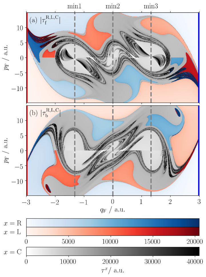
Figure 7: Phase space representation of the ATI values for the 1D ketene model in an external field for the (a) forward $\tau_{\mathrm{f}}^{\mathrm{R,L,C}}$ and (b) backward $\tau_{\mathrm{b}}^{\mathrm{R,L,C}}$ time propagation. The color for each initial condition is chosen according to the absorbed position: $q_{\mathrm{F}}=-3$ (red), $q_{\mathrm{F}}=3$ (blue), and the initial coordinate with the same velocity sign (gray), as also shown in Fig.5.

We now demonstrate the usefulness of the ATI for the 1 DoF (Eq. (32)) and 3 DoF (Eq. (38)) ketene models. To this end, we use the visualization scheme explained in relation to Figs. 2 and 5. In Fig. 7, we show the result for the 1 DoF model marking each location with the value of the ATI for trajectories starting at that point and ending when they reach $|q_{\mathrm{F}}|=3$. As can be seen, for the forward time propagation, trajectories starting from initial conditions at $q_{\mathrm{F}}=-3,p_{\mathrm{F}}<0$ ($q_{\mathrm{F}}=3,p_{\mathrm{F}}>0$) have the lightest red (blue) color, in Fig. 7a, because these trajectories are absorbed immediately. Similarly, in Fig. 7b, trajectories starting at $q_{\mathrm{F}}=-3,p_{\mathrm{F}}>0$ ($q_{\mathrm{F}}=3,p_{\mathrm{F}}<0$) have the lightest red (blue) color. The areas with large $|p_{\mathrm{F}}|$, not plotted in the figure, correspond to ballistic trajectories that will not be trapped in the wells. The areas which have darker reds and blues correspond to trajectories that bounce back at the right and left external saddles $q_{\mathrm{F}}=2.8(=-2.8)$, respectively, and then escape from it without a recurrence. These areas always present darker colors at the edge, due to the presence of asymptotic (long-time) trajectories. There is a line of discontinuities at $p_{\mathrm{F}}=0$ due to the application of the recurrent condition, and is an artifact of the way we define absorption. The gray colored area results from the limitation in the propagation time used in our calculation to be insufficiently long to resolve these areas in terms of red and blue absorbing boundaries. For example, in the case when we apply the recurrent condition for the later time starting at $\omega t=14\pi$, some gray areas in Fig. 7a are colored as it is seen in Fig. 1b. We show below that the manifold-like structures in this area are in fact a manifold.

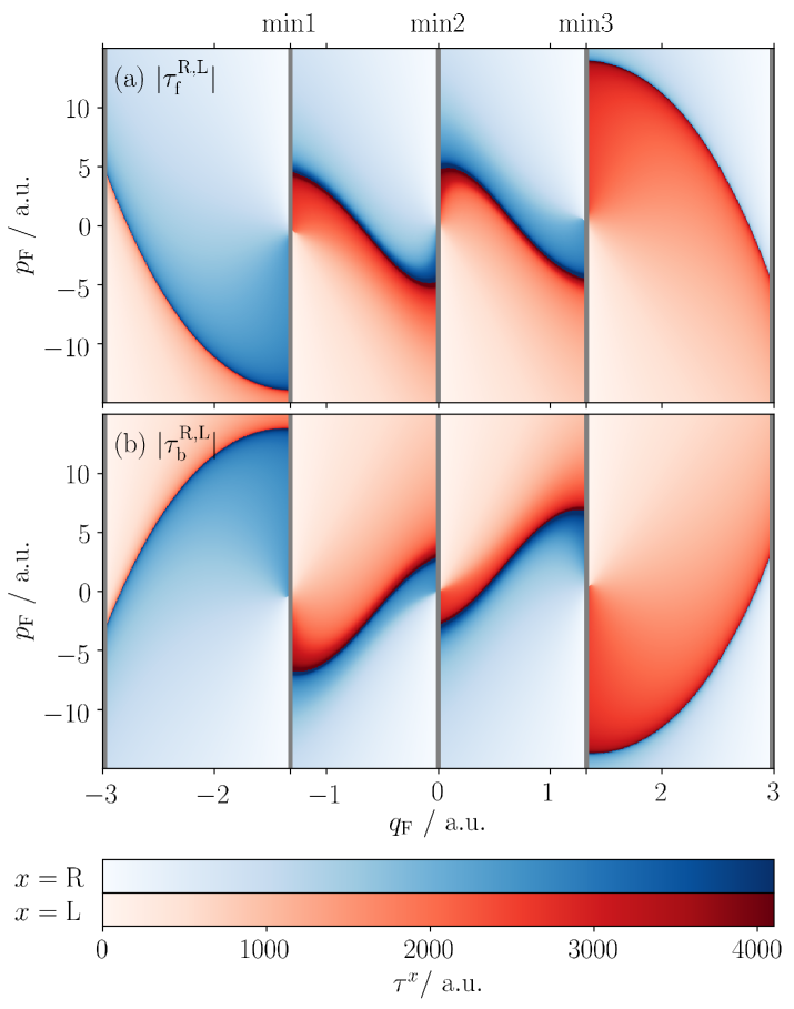
Figure 8: Phase space representation of the ATI values for the 1D ketene model in an external field for the (a) forward $\tau_{\mathrm{f}}^{\mathrm{R,L}}$ and (b) backward $\tau_{\mathrm{b}}^{\mathrm{R,L}}$ time propagation. The color for each initial condition is chosen according to the absorbed position: left (red), and right (blue). The absorbing boundaries are located at $q_{\mathrm{F}}=-3$, the local minima (min1, min2, min3), and $q_{\mathrm{F}}=3$ are shown in gray corresponding to the red or blue boundaries of Fig. 5 within a given region.

As discussed in Sec. II, the use of the ATI to locate the stable or unstable manifold of a NHIM in a given region becomes unclear when the region contains more than one NHIM because of the challenge in assigning asymptotic behavior to a particular origin. To address this challenge, we consider the effect of inserting additional absorbing boundaries. For example, the results corresponding to the insertion of absorbing boundaries at the potential energy minima (min1, min2, min3 defined in the caption to Fig. 1 are shown in Fig. 8. The identification of the manifold results from propagation of trajectories that are 5 times smaller than the previous figure (as indicated by the smaller ATI values). The increased efficiency results from the fact that we do not need to use the recurrent condition due to the presence of the additional absorbing conditions. We are thus able to observe the manifolds that mediate internal mechanism in addition to the escaping process. Below in Subsec. IV.3 and Appendix D, we demonstrate the resolution of the entire phase space using this approach.

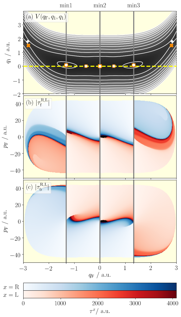
Figure 9: (a) Potential energy surface for the reduced 3D ketene model on the $q_{2}=q_{1}$ plane. The white filled-circle symbols (plus symbols) indicate the position of minima (saddles) on the plane, and the orange filled-square symbols (times symbols) correspond to projected minima (saddles). The yellow dashed line is the surface of initial conditions. The middle and the bottom panels are the forward (b), and backward (c) ATIs on the $q_{1}=q_{2}=0$ plane. The absorbing boundaries are the same as in Fig. 8 except for the outer most boundaries that are now located at $q_{\mathrm{F}}=\pm 4$. The light yellow areas in (b) and (c) are on the outside of the initial energy $E=0.1~{}\mathrm{a.u.}$.

The ATI can be used in systems that are stochastic/non-autonomous, with multiple DoFs, and without need for an a priori reaction coordinate. To demonstrate this fact, we present a visualization of ATI for the 3 DoFs ketene model coupled to a Langevin bath. In Fig. 9a and Fig. 10a, the $q_{1}=q_{2}$ slice contour plot of the potential energy surface is shown. The white filled-circles (plus symbols) are local minima (saddles) on the slice, and the orange filled-squares (times symbols) are projected local minima (saddles). In Fig. 9, the initial conditions are prepared on the yellow dashed line with positive out-of-slice velocity and constant energy $E=0.1~{}\mathrm{a.u.}$ ($q_{1}=q_{2}=0$ and $p_{1}=p_{2}>0$). The absorbing conditions are the same as in Fig. 8 except the outermost boundaries $q_{\mathrm{F}}=\pm 3$ that are now $q_{\mathrm{F}}=\pm 4$ and which are not shown in the figure. This change in the outer boundaries was necessitated by the observed discontinuities in the ATI as implemented with the narrower absorbing boundaries at $q_{\mathrm{F}}=\pm 3$, possibly due to the overlap of the boundary with the NHIMs. Since we use the fixed initial energy, there is an upper and lower limit for the velocity not seen in Fig. 8. In comparison with Fig. 8, there is no change in the timescale of the ATIs in Fig. 9 because the increase of the DoFs does not affect the timescale of the motion.

Although the reaction coordinate on the potential energy function is curved, we are still able to locate the reactivity boundaries on each cell According to the result of the ATI, the initial conditions are best given by $p_{1}>0$ ($p_{1}<0$) for positive (negative) time integration. This fact can be observed from the backward time propagation case, shown in the left cell of Fig. 9c. Therein, we mostly observe bounce back trajectories from the right (min1) shown by blue colors. This occurs since we take $p_{1}>0$. As a consequence, trajectories have opposite velocity along $p_{1}$ in comparison with the trajectories sliding down from the left external saddle. The right cell of Fig. 9c has similar behavior due to the symmetry of the potential energy surface.

The black areas in the middle right cells of Figs. 9b and 9c correspond to trajectories that have not finished in the computation time $t=10^{5}$. Those trajectories are, in fact, those which stay vibrating on the initial coordinate $q_{\mathrm{F}}$ plane, possibly in the attraction basin of the fixed points/invariant manifold. There is a line in Fig. 9c (center cells) of small discontinuities which is an artifact of the absorbing boundaries. The reactivity boundary must have a singular value of $\tau$, otherwise it appears due to an inappropriate absorbing boundary.

Figure 10: (a) The potential energy surface of reduced 3D ketene model on $q_{1}=q_{2}$ plane (see Fig. 9) and superimposed absorbing boundaries $A$ (red line) and $B$ (blue line). The green dashed line corresponds to $\tilde{q}_{1}=0$. (b) forward and (c) backward ATIs of reduced 3D ketene model in a Langevin bath with initial conditions on surface $B$ with $q_{1}=q_{2}$. The light yellow areas in (b) and (c) are the outside of the initial energy $E=0.1~{}\mathrm{a.u.}$.

Beside the absorbing boundaries considered in Fig. 9, for the multiple DoFs systems, one can use a variety of absorbing boundaries, such as a boundary transverse to the reaction path or the one used in the reaction island theory.Ozorio de Almeida et al. (1990) In Fig. 10, we present the result for the absorbing boundaries A (red) and B (blue) that enclose the left external saddle point, and are given by $q_{1}=q_{\mathrm{F}}+8$ and $q_{1}=q_{\mathrm{F}}+3$ respectively. The initial conditions are prepared on the boundary B with $q_{1}=q_{2}$ by using the mass-weighted coordinates along B ($\tilde{q}_{\parallel}$) and orthogonal to B ($\tilde{q}_{\perp}$). We define the zero axis ($\tilde{q}_{1}=0$) by $q_{1}=-q_{\mathrm{F}}-1$ (green dashed line), which is along the coordinate $\tilde{q}_{\perp}$. Thus, the origin $\tilde{q}_{1}=0$ of Fig. 10 is at $(q_{\mathrm{F}},q_{1},q_{2})=(-2,1,1)$, which is the crossing point of the line B and the dashed green line. Here we use a Lagrangian transformation to obtain $\tilde{q}_{\parallel}$ and $\tilde{q}_{\perp}$ under the condition $p_{1}=p_{2}$. The result for the ATI is shown in Figs. 10b and 10c. In these panels, the reactivity boundary between blue and red area can be located even in the challenging case presented by a Langevin bath. Initial conditions with $\tilde{q}_{1}<0$ and $\tilde{p}_{1}<0$ ($\tilde{p}_{1}>0$) corresponding mostly to reacting trajectories (red) in the forward or backward time propagation as seen in Fig. 10b (Fig. 10c). This is because these initial conditions are closer to the left external saddle and have velocities ahead to or from this saddle, respectively.

IV.3 Turnstile and Reaction Path

Figure 11: The turnstile (reaction pathway) of each NHIM (saddle), mediated by the manifolds obtained at phase $\omega t\equiv 0\pmod{2\pi}$ of the 1D ketene model driven by an external force. The stable (blue, cyan) and unstable (red, orange) manifolds are drawn up to $|\omega t|=8\pi$. The manifolds associated with the saddles for left external (a), right external (b), left internal (g) and right internal (h) are shown in (c), (d), (e), (f) respectively. The colors of the manifolds become lighter, as $|t|$ increases. Left and right panels correspond to exiting and entering trajectories, respectively, Coherent sets of these trajectories are marked in gray, with increasingly lighter shades indicating later phases, that are enclosed by the stable and unstable manifold.

Table 4: Four types of phase space regions separated by stable and unstable manifolds

		stable manifold
		inside	outside
unstable	inside	(1) staying inside	(2) entering into
manifold	outside	(3) exiting from	(4) staying outside

We now demonstrate a way to use the manifolds obtained by NBC-ATI in Sec. III.2 in the context of turnstileMackay et al. (1984) or lobe dynamics.Wiggins (1990) As discussed in Fig. 2, the stable and unstable manifolds is the destination and origin dividing boundaries respectively, of the dynamics. The areas divided by the reactivity boundaries are categorized into four types (see Table 4): trajectories that are (1) staying inside, (2) entering into, (3) exiting from, and (4) staying outside the trapping area (a chemical state). Among the four types, an area which encloses the reaction pathway is categorized into (2) or (3) and corresponds to a time slice of the pathway.

In Fig. 11, the manifolds produced from each cell in Fig. 8 are shown through the superposition of the manifolds at the phases $|\omega t|=2\pi M(M=0,\dots,4)$ (see Appendix D). These manifolds correspond to the stable (blue, cyan) and the unstable (red, orange) manifolds of the NHIM in each cell. To expose the reaction mediated by these manifolds, we draw a set of trajectories prepared in an enclosed area (gray). These trajectories move coherently from one enclosed area to another and are shown (stroboscopically) at $\Delta t=2\pi/\omega$ time intervals with changing strength of its color. Darker color indicate points captured in earlier time periods. As the color becomes lighter, the set of trajectories goes out of (or into) the trapped area in the left (or right) column in Fig. 11. Although, we illustrate trajectories in a few selected area, this should suffice to observe that the dynamics are mediated by the manifolds as expected.

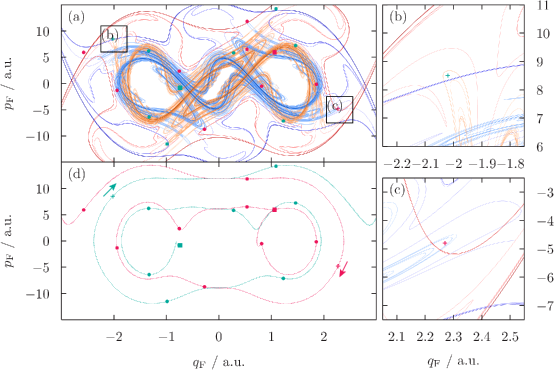
Figure 12: The intersections of the internal and external stable/unstable manifolds of ketene 1 D with external field. (a) Superposition of manifolds at phase $\omega t\equiv 0\pmod{2\pi}$ up to $|\omega t|=14\pi$ which partially shown in Fig. 11. (b) and (c) Magnifications of areas marked in (a) where we sample the initial conditions of trajectories (plus symbols). (d) The sampled entering (pink dotted line) and exiting (green dotted line) trajectories. The plus symbols, filled-squares, and filled-circles are time-slices at the phase $\omega t\equiv 0~{}\pmod{2\pi}$ of trajectories (dotted lines).

The manifolds in the left and right column of Fig. 11 are the same but the initial gray-colored areas are different as they correspond to the time slice of the exiting and entering reaction paths, respectively. They illustrate the last or first few steps of the reaction pathways. One can combine these pictures to see a reaction pathway exiting into (entering from) the internal well from (to) the outside of the observed area. Such a pathway must be explained by the intersection of the reaction pathways mediated by internal ((b) and (c)) and external ((a) and (d)) manifolds in Fig. 11. To see the intersection, we draw the manifolds up to the phase $M=7$ in Fig. 12. We uncover two initial conditions that are enclosed by the both internal and external manifolds in Fig. 12b and c respectively. The resulting pink (green) trajectory shows that pathway comes into (goes out) the internal well directly from (toward) outside. These correspond to a case in which there is a fast cooling-down (fast excitation) process due to the presence of an external field. However, from the size of the enclosing area of the initial conditions in Fig. 12b and c, one can also observe that the amount of such coherent initial conditions are small indicating that the event is pretty rare. Thus, there is a time scale separation for transitions between internal trapping and external trapping trajectories since the former has less energy than the latter.

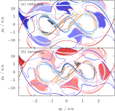
Figure 13: (a) The exiting trajectories of 1D ketene shown in Fig. 12(d) superimposed on the associated coherent set of trajectories shown in Fig. 11 (c) (gray) and (g) (blue). (b) the same for the entering trajectory superimposed on the associated coherent set of trajectories shown in Fig. 11 (b) (red) and (f) (red). The color of the set of the trajectories get lighter when the time period is later.

In Fig. 13, we interpret the trajectories of Fig 12 in the context of turnstiles. In Fig. 13a, the limit point —shown as a green filled-square— is in the area colored by the darkest gray. As time progresses, the green filled-circles move into ever lighter colored areas in the Poincaré map. In the first three periods, the circles from the green filled-square all moved into areas shaded with increasingly lighter gray. Starting with the second period, the circles also move into blue areas. These later circles move into areas with increasingly lighter blue shades until they move outside of the figure. Similarly, the pink trajectory starting from a different point in the phase space experiences a series of gray and red areas in Fig. 13b upon application of the Poincaré map. Therefore, the trajectories sampled at the points in Fig. 12 are successfully identified by the intersection of the reaction pathways mediated by internal ((b) and (c)) and external ((a) and (d)) manifolds in Fig. 11.

Finally, let us revisit Fig. 1. The ATI shown in Fig. 1b was computed without applying the absorption of recurrent trajectories until $|\omega t|>7\times 2\pi$. The choice for this max time is in agreement with the number $(=7)$ of periodic lobes (red or blue colored areas) of the coherent trajectories that we followed in Fig. 13. The coherent structures, mediated by the reactivity boundaries and revealed by the NBC-ATI method, are clearly visible in Fig. 1b because we compute ATI values for longer times than those shown Fig. 7. The yellow lines are the superpositions of the external stable manifolds that are also shown in Fig. 12a as blue lines. These coherent structures agree with the those shown in Fig. 1c obtained directly through the use of global manifolds. That is, the phase space skeletons are correctly extracted by the NBC-ATI algorithm. It leads to consistent and correct implications on the dynamics. Therefore, all the information about reactivity is extracted only from the manifolds obtained by the NBC-ATI algorithm.

V Discussion

Here, we analyze the possible use of the NBC-ATI method to describe more general chemical reactions based on our findings from the analysis of the 1D and 3D ketene models under various coupling conditions. In Fig. 9 and Fig. 10, we showed a 2D slice of the ATI in the 3 DoFs phase space. To obtain them in the full phase space, naively one needs to achieve it for all the remaining slices. However, as we showed in Sec. IV.3, one can use a periodic identity of the dynamics to obtain samples by integrating across several period(s) of time. This sampling is more efficient for autonomous systems because the phase space is identical for all time. Although this type of identity reduces computational costs, the minimum computation costs must be proportional to the dimension of the manifold in any numerical analysis. This is because even if we just uniformly sample a known $n$-dimensional manifold, a number of points proportional to the order of the power $n$ is needed. This is a fundamental limitation of numerical sampling techniques that perturbation theories do not suffer.

Unlike in autonomous or periodic dynamical systems, there exists no natural Poincaré map in systems driven by aperiodic or stochastic differential equations. Hence, to see the reactivity boundaries at another time, one does not have any resource beyond the time-propagated manifold. In addition, for stochastic differential equations, the computational cost is larger because the integrators available for such systems are not as efficient as those for an ODE. To achieve a given resolution in the time-propagated manifold, the resolutions used within steps of the NBC-ATI must be chosen carefully ensuring that the computation is efficient. Due to the nature of a trajectory on a stable or unstable manifold, the distance between adjacent straddling pairs will exponentially increase by the time backward or forward propagation, respectively. Nevertheless, the weighted samplingNagahata et al. (2013b) is known to improve the efficiency. Since the NHIM and their stable and unstable manifolds are smooth, interpolation between the straddling pairs will reduce computational cost to some extent. For engineering purposes, this types of solutions can improve efficiency, although, what types of interpolation are allowed to use is still in question. Although the NHIM and its stable and unstable manifolds are of great importance, there is no guarantee that that reactivity is always mediated by them. It appears in the study of a reaction associated with higher index saddlesNagahata et al. (2013b, a) that the manifold, which is not orthogonal to the most repulsive nor attractive direction, can produce reactivity boundaries. However, one should be careful to correctly ascribe the physical interpretation of these reactivity boundaries. They may not persist under perturbation. That is, a small perturbation e.g., a small difference of potential energy surface, may introduce a large dynamical difference. The NBC-ATI also provides a useful reference for determining which terms in perturbation theories should be retained. For example, normal form theories are known to be asymptotic series which necessarily diverge if one includes all terms in the expansion.

VI Conclusion

In this paper, we have presented a formulation for the ATI and an identification of reactivity boundariesNagahata et al. (2013b) based on dynamical systems theory by revisiting the reactivity map.Wall et al. (1958, 1961); Wall and Porter (1963); Wright et al. (1975, 1976); Wright and Tan (1977); Wright (1978); Laidler et al. (1977); Tan et al. (1977) To this end, we developed the NBC-ATI method which effectively requires computational resources that are proportional to the dimensionality of the manifolds. We demonstrate the feasibility and efficiency of this approach on a reduced-dimensional ketene modelGezelter and Miller (1995) in 1D with external field, and in 3D coupled to a Langevin bath. The NBC-ATI method can address irregular reactions which are not accessible to conventional perturbation theories or other types of numerical analysis. Examples include the existence of roaming pathways,Bowman and Shepler (2011); Mauguière et al. (2017) bifurcation of the periodic orbit dividing surface,Pollak and Pechukas (1978); Li et al. (2006) dynamical switching of the reaction coordinate,Teramoto et al. (2011) and a reaction associated with higher index saddle(s).Nagahata et al. (2013b, a)

In the reduced 1D ketene model, we obtained complex reaction paths based on turnstiles.Mackay et al. (1984) The turnstiles consist of stable and unstable manifolds associated with the NHIMs around the four potential energy saddle points. We find the internal trapping area in a chaotic sea corresponding to the two formylmethylenes and oxirene conformations. Using these phase space structures, we identified and characterized rare trajectories which are trapped by and escape from the internal wells in a short time. We thus demonstrated that our method has sufficient accuracy to reproduce the conventional analysis when it is accessible, and generalizes to reactions with more complex reaction geometry as listed above.

We have shown the applicability of the NBC-ATI method for stochastic and higher dimensional systems through an application to a reduced 3D ketene model. We found that if one can identify an area which includes the NHIM or an asymptotic manifold $\mathcal{M}_{\mathrm{asym}}$ as a seed of the reactivity boundaries,Nagahata et al. (2013b) then the ATI still allows us to identify the reactivity boundaries in stochastic and higher dimensional systems. Besides the advantage of reduced computational costs, the ATI allows us to identify structures associated with the reaction path in cases which are beyond reach to the conventional perturbation theories and numerical analysis.

Appendix A NHIM persistence theorem

The NHIM is a multidimensional generalization of a hyperbolic fixed point such as that associated with the saddle point —viz the naive TS— in a chemical reaction. Here, we recapitulate the statement of the theorem for the persistence of the NHIM under perturbations as originally proven by Fenichel,Fenichel (1972) and generalized by others.Hirsch et al. (1977); Eldering (2013) For simplicity, we call this the NHIM persistence theorem.

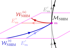
Figure A.1: Invariant splitting at $\bm{m}\in\mathcal{M}_{\mathrm{NHIM}}$: $E^{\mathrm{c}}_{\bm{m}}\otimes E^{\mathrm{s}}_{\bm{m}}\otimes E^{\mathrm{u}}_{\bm{m}}$ and its relation with $\mathcal{M}_{\mathrm{NHIM}}$, $\mathcal{W}_{\mathrm{NHIM}}^{\mathrm{(s)}}$, and $\mathcal{W}_{\mathrm{NHIM}}^{\mathrm{(u)}}$.

Suppose that in a given system, we have identified a smooth Riemannian manifold $\mathcal{Q}$, a flow on $\mathcal{Q}$: $\bm{\phi}^{t}\in C^{k}\ (r\geq 1)$, and a compact submanifold of $\mathcal{Q}$: $\mathcal{M}_{\mathrm{NHIM}}$. This manifold, $\mathcal{M}_{\mathrm{NHIM}}$, is NHIM NHIM when:

1. $\mathcal{M}_{\mathrm{NHIM}}$ is invariant, i.e., $\bm{\phi}^{t}(\mathcal{M}_{\mathrm{NHIM}})=\mathcal{M}_{\mathrm{NHIM}}$,

2. There exists continuous splitting for $\forall\bm{m}\in\mathcal{M}_{\mathrm{NHIM}}$,

   $$T_{\bm{m}}\mathcal{Q}=E^{\mathrm{c}}_{\bm{m}}\otimes E^{\mathrm{s}}_{\bm{m}}\otimes E^{\mathrm{u}}_{\bm{m}},$$ (39)

   of the tangent bundle of $\mathcal{Q}$ at $\bm{m}$ with globally bounded, continuous associated projections: $\bm{\pi}_{\bm{m}}^{\mathrm{c}}$, $\bm{\pi}_{\bm{m}}^{\mathrm{s}}$, and $\bm{\pi}_{\bm{m}}^{\mathrm{u}}$ such that splitting is invariant under the linearized flow

   $$D_{\bm{m}}\bm{\phi}^{t}(E^{x}_{\bm{m}})=E^{x}_{D_{\bm{m}}\bm{\phi}^{t}(\bm{m})}$$ (40)

   for $\forall\bm{x}\in E^{x}~{}(x=\mathrm{c,s,u})$ where $E^{\mathrm{c}}_{\bm{m}}=T_{\bm{m}}\mathcal{M}_{\mathrm{NHIM}}$ and $D_{\bm{m}}\bm{\phi}^{t}$ is differential of $\bm{\phi}^{t}$ at $\bm{m}$, e.g. the flow determined by the normal mode for the Hamiltonian systems.

3. There exists constants $-\lambda_{\bm{m},\mathrm{s}}<-\lambda_{\bm{m},\mathrm{c}}\leq 0\leq\lambda_{\bm{m},\mathrm{c}}<\lambda_{\bm{m},\mathrm{u}}$, $c_{\bm{m},\mathrm{c}},c_{\bm{m},\mathrm{s}},c_{\bm{m},\mathrm{u}}\geq 1$, such that for the matrix $D_{\bm{m}}\bm{\phi}^{t}={(\partial_{x_{i}}\phi^{t}_{j}(\bm{x})|_{\bm{x}=\bm{m}})}_{ij}$

   $$\forall t,\ \bm{x}\in E_{\bm{m}}^{\mathrm{c}}:$$

   $$\norm{D_{\bm{m}}\bm{\phi}^{t}\bm{\pi}_{\bm{m}}^{\mathrm{c}}(\bm{x})} \leq c_{\bm{m},\mathrm{c}}\mathrm{e}^{\lambda_{\bm{m},\mathrm{c}}|t|}\norm{\bm{\pi}_{\bm{m}}^{\mathrm{c}}(\bm{x})},$$

   $$\forall t\geq 0,\ \bm{x}\in E_{\bm{m}}^{\mathrm{s}} :$$

   $$\norm{D_{\bm{m}}\bm{\phi}^{t}\bm{\pi}_{\bm{m}}^{\mathrm{s}}(\bm{x})} \leq c_{\bm{m},\mathrm{s}}\mathrm{e}^{-\lambda_{\bm{m},\mathrm{s}}t}\norm{\bm{\pi}_{\bm{m}}^{\mathrm{s}}(\bm{x})},$$

   $$\forall t\leq 0,\ \bm{x}\in E_{\bm{m}}^{\mathrm{u}}:$$

   $$\norm{D_{\bm{m}}\bm{\phi}^{t}\bm{\pi}_{\bm{m}}^{\mathrm{u}}(\bm{x})} \leq c_{\bm{m},\mathrm{u}}\mathrm{e}^{\lambda_{\bm{m},\mathrm{u}}t}\norm{\bm{\pi}_{\bm{m}}^{\mathrm{u}}(\bm{x})}.$$ (43)

For the sake of simplicity, we restrict the constants $\lambda_{\bm{m},x}\ (x=\mathrm{c,s,u})$ to the absolute condition:Hirsch et al. (1977) $\lambda_{x}=\sup_{\bm{m}}\lambda_{\bm{m},x}$. Under this absolute condition, the condition 3 for $\bm{\phi}^{t}\in C^{k}$ can be rewritten with a gap $r\geq 1$ by $-\lambda_{\mathrm{s}}<-r\lambda_{\mathrm{c}}\leq 0\leq r\lambda_{\mathrm{c}}<\lambda_{\mathrm{u}}$. Then, $\mathcal{M}_{\mathrm{NHIM}}$ is $C^{k}$ for some $k\leq r$, and the manifold is called an eventually and absolutely $k$-NHIM.Eldering (2013) For this $k$-NHIM, there exists a vector field of $\tilde{\bm{\phi}}^{t}$ and a manifold $\tilde{\mathcal{M}}_{\mathrm{NHIM}}$ that are $C^{k}$–close, that is, the manifold remains a $k$-NHIM or persists under $C^{k}$ perturbation.

The theorem was extended to non-compact NHIMs.Eldering (2013) In this case, $\mathcal{Q}$ is a bounded geometry and $C^{k}$ is accordingly changed into $C^{k.x}_{b,u}$. (See Ref. Eldering, 2013 for those definitions.)

Appendix B The NHIM Persistence Theorem for RDSs

For each $d$-dimensional stochastic path instance $\bm{B}_{t}$, one can uniquely obtain a $d$-dimensional, $t$-continuous function $\bm{\omega}(t)$ —as defined in Appendix C)— that is associated with the saddle point at each instance of time $t$, and for which we are free to initialize at $\bm{\omega}(0)=0$. $\bm{\omega}(t)$ is a generalization of the so-called TS trajectoryBartsch et al. (2005) discussed in the main text. A probability distribution can then be defined for the bundle of instances $\bm{\omega}$ from the probability distribution of $\bm{B}_{t}$, Thus, the event space $\Omega$, which contains this bundle, is defined by the corresponding $d$-dimensional $t$-continuous functions $C(\mathbb{R},\mathbb{R}^{d})$:

$$\Omega=\left\{\bm{\omega}\middle|\bm{\omega}\in C(\mathbb{R},\mathbb{R}^{d}),\bm{\omega}(0)=0\right\}.$$ (44)

We define the Wiener shift $\theta_{s}$, and a cocycle $\bm{\phi}^{t}_{\bm{\omega}}$ —that is a random invariant manifold $\mathcal{M}(\bm{\omega})$— such that, $\bm{\phi}^{t}_{\bm{\omega}}(\mathcal{M}(\bm{\omega}))=\mathcal{M}(\theta_{t}\bm{\omega})$. The persistence of the compact NHIM theorem for RDS holdsLi et al. (2013) for these invariant manifolds. Let us enumerate the differences in the expression of the persistence theorems between Refs. Eldering, 2013; Li et al., 2013.

1. The following are all $\bm{\omega}$ dependent: $\mathcal{W}_{\mathrm{NHIM}}^{\mathrm{(s)}}(\bm{\omega})$, $\mathcal{W}_{\mathrm{NHIM}}^{\mathrm{(u)}}(\bm{\omega})$, $E^{x}(\bm{\omega})$, $\bm{\pi}^{x}_{\bm{m}}(\bm{\omega})$, $c_{\bm{m},x}(\bm{\omega})$, and $\lambda_{\bm{m},x}(\bm{\omega})$ $(x=\mathrm{s,u,c})$, as well as $\mathcal{M}_{\mathrm{NHIM}}(\bm{\omega})$, and $\bm{\phi}^{t}_{\bm{\omega}}$.

2. Eq. (40) holds only for $E^{x}~{}(x=\mathrm{c,u})$. For $E^{\mathrm{s}}$,

   $$D_{\bm{m}}\bm{\phi}^{t}_{\bm{\omega}}(E^{\mathrm{s}}_{\bm{m}}(\bm{\omega}))\subset E^{\mathrm{s}}_{D_{\bm{m}}\bm{\phi}^{t}_{\bm{\omega}}(\bm{m})}(\theta_{t}\bm{\omega}).$$ (45)

3. (Persistence) $\mathcal{M}_{\mathrm{NHIM}}(\bm{\omega})$ is a $1$-normally hyperbolic random invariant manifold.

However, $\mathcal{M}_{\mathrm{NHIM}}(\bm{\omega})$ is still $C^{k}~{}(r\geq k)$ smooth when $\bm{\phi}^{t}_{\bm{\omega}}$ is $C^{k}$ and $-\lambda_{\mathrm{s}}(\bm{\omega})<-r\lambda_{\mathrm{c}}(\bm{\omega})<0<r\lambda_{\mathrm{c}}(\bm{\omega})<\lambda_{\mathrm{u}}(\bm{\omega})$ for $\lambda_{x}(\bm{\omega})=\sup_{\bm{m}}\lambda_{\bm{m},x}(\bm{\omega})$. However, these differences do not mean that the persistence in the NHIM theorem for RDS does not hold for more relaxed conditions.

Appendix C RDE from SDE

For the Langevin type SDEs, one can obtain its RDEs from the use of a stationary orbitDuan (2015). Suppose, SDE SDE with a Wiener process $W_{t}\sim\mathcal{N}(0,t)$,

$$\differential X_{t}=(aX_{t}+b(X_{t}))\differential t+c\differential W_{t},$$ (46)

is transformed by a stationary orbit $\eta_{t}$, such that,

$$\differential\eta_{t}=a\eta_{t}\differential t+c\differential W_{t},$$ (47)

thus for $t_{0}\leq t\leq t_{1}$,

$$\derivative*{(X_{t}-\eta_{t})}{t}=(ax+b(X_{t})),$$ (48)

$$\eta_{t}=\begin{cases}{}\mathrm{e}^{a(t-t_{0})}\eta_{t_{0}}+c\int_{t_{0}}^{t}\mathrm{e}^{-a(s-t)}\differential W_{s}\\ \mathrm{e}^{a(t-t_{1})}\eta_{t_{1}}-c\int_{t}^{t_{1}}\mathrm{e}^{-a(s-t)}\differential W_{s}\\ \end{cases},$$ (49)

where we use Itô’s lemma: $\differential(\mathrm{e}^{-at}\eta_{t})=\differential(\mathrm{e}^{-at})\eta_{t}+\mathrm{e}^{-at}\differential\eta_{t}+\differential(\mathrm{e}^{-at})\differential\eta_{t}=\mathrm{e}^{-at}(-a\differential t+\differential\eta_{t})$, and we only wrote terms with order $\differential t$ or less. When $x=X-\eta$ such that $x(t)=X_{t}$ and $\omega(t):=\eta_{t}$ with $\eta_{0}=0$, one obtain a corresponding RDE,

$$\dot{x}=(ax+b(x+\theta_{t}\omega)).$$ (50)

For this equation, one have the corresponding RDS. The similar discussion can be made for the higher dimensional, Langevin type (Eq. (46)) systems. Here one can observe the TS trajectory $\eta_{t}^{\ddagger}$,

$$\eta_{t}^{\ddagger}=\begin{cases}{}-c\int_{-\infty}^{t}\mathrm{e}^{-a(s-t)}\differential W_{s}~{}(a<0)\\ c\int_{t}^{\infty}\mathrm{e}^{-a(s-t)}\differential W_{s}~{}(a>0)\end{cases},$$ (51)

is a special case of the stationary orbit Eq. (47) by replacing $t_{0}\to-\infty,t_{1}\to\infty$ in Eq. (49).

Appendix D Sampling the Reactivity Boundary

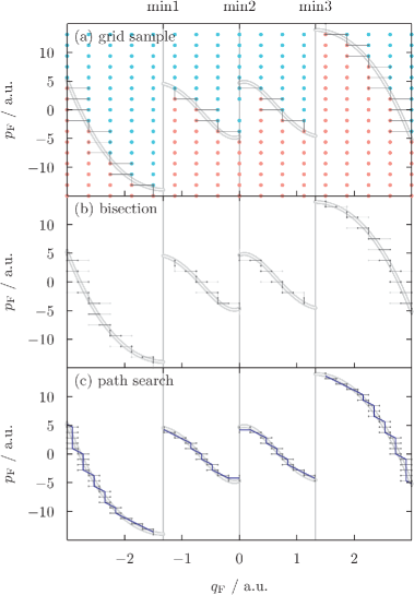
Figure D.2: Step-by-step visualization of the algorithm to sample neighboring points of the forward-time reactivity boundaries in ketene 1 D with external force. The solution lines are shown in light gray. Straddling pairs of the forward-time reactivity boundaries (gray links with dots). (a) The initial conditions absorbed at right (left) of each cell divided by the coordinate position of $q_{\mathrm{F}}=-3$, min1, min2, min3, and $q_{\mathrm{F}}=3$ after positive time integration (blue (red) dots). (b) The initial straddling pairs before (after) the bisection method applied (light gray (dark gray)). (c) The result of the path search algorithm (see Fig. 6) and its midpoint approximation of the neighboring points (blue).

In this subsection, we demonstrate how the algorithm, introduced in Sec. III and Fig. 6, works in 1 D ketene with external force (Eq. (32)). Ideally, it is better to just locate the asymptotic trajectories, and this can be achieved by the perturbation theories. However, for irregular reactions, there could be a case for which the theories are not applicable, and need to use numerical investigation until an applicable theory is developed.

The key step in the algorithm is the minimization of the uniform sampling. In Fig. D.2, we visualize the locating process. Fig. D.2a, shows initial conditions by $(2^{4}+1)\times(2^{4}+1)$ grid sampling. This produce more than one sample for each area divided by the reactivity boundaries thus the sampling is sufficient as seeds for the algorithm. In the next step (Fig. D.2b), we apply the bisection method until when the demanded number of samples are obtained from the resolution. In the figure, the bisection method is only applied once for the visualization purpose. Then in the bottom figure, the results of the search on the resolution is given by the use of the algorithm we introduced in Fig. 6. Finally, one can apply the bisection method for each pair until when the demanded precision is achieved.

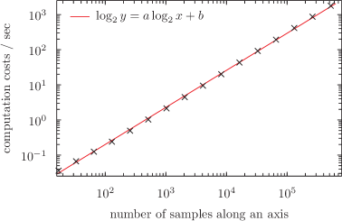
Figure D.3: Computation cost in seconds as a function of the sampling resolution (see also Fig. D.2). The initial grid size is $(2^{4}+1)\times(2^{4}+1)$. The first bisection is applied up to $(2^{N_{\mathrm{res}}}+1)\times(2^{N_{\mathrm{res}}}+1)$ grid resolution where $(2^{N_{\mathrm{res}}}+1)$ is value of the $x$-axis. After the path search, the bisection method is applied again up to $(2^{30}+1)\times(2^{30}+1)$ grid resolution. The results are shown as cross symbols. The least square fit is $\log_{2}{y}=1.0558\times\log_{2}{x}+9.3353$ (red line).

Fig. D.3 shows the computational costs of the different sampling resolutions. That is, when we chose the sampling resolution $(2^{N_{\mathrm{res}}}+1)\times(2^{N_{\mathrm{res}}}+1)$ (Fig. D.2-bisection), and chose the precision achieved by $(2^{30}+1)\times(2^{30}+1)$ grid, the $x$–axis of the figure is given by $2^{N_{\mathrm{res}}}+1$, and $y$–axis is given by actual computational time observed by std::clock, which is implemented in the C++ standard template library. In the $\log$-$\log$ plot, the cost is an almost linear-order increase over the sampling resolution. The order is able to estimate by the parameter $a\approx 1$ of the fitting function $\log_{2}{y}=a\log_{2}{x}+b$ where $(a,b)=(1.0558,9.3353)$. Hence, the algorithm effectively decreases one polynomial order of the computational cost from uniform samplings. This is more efficient than the LD calculation. Notice that the computation cost for the worst case is still second order because one does not know the shape of the reactivity boundary before hands and there is a case that the boundaries are densely existed.

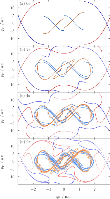
Figure D.4: The reactivity boundaries at phase $|\omega t|=0,2\pi,4\pi,6\pi$ (a-d) obtained by a method explained in Fig. D.2 with the resolution given by $N_{\mathrm{res}}=16$. The reactivity boundaries are corresponding to stable (blue, cyan) and unstable (red, orange) manifolds. The colors of the manifolds get lighter as $|t|$ increases.

If the external field is periodic, for the frequency $\omega$ of the periodic field, the phase space at $t=0$ is identical when $\omega t\equiv 0\pmod{2\pi}$. To take this advantage, one can propagate time $t$ and get more samples. In Fig. D.4, we depict the results of time ($|\omega t|=0,2\pi,4\pi,6\pi$) integrations of the straddling pairs of manifolds obtained by the algorithm. In the figure, the propagated sample points (gray), midpoint estimation of each pair, and the line between the estimations (red or orange for $\tau_{\mathrm{b}}$, blue or cyan for $\tau_{\mathrm{f}}$) are shown. The strength of each color is proportional to the phase $|\omega t|$. For example for the phase $|\omega t|=2\pi M$, $M=0$ is darkest, and the color get lighter for larger $M$. We employ $N=12$ for the sampling resolution $(2^{N_{\mathrm{res}}}+1)\times(2^{N_{\mathrm{res}}}+1)$ of the algorithm. The gray dots and lines are not visible because the estimation is precise, and those are overwritten by midpoint estimations. The lines between the midpoints are given when the two consecutive midpoints have less than a certain distance on the figure. The disconnection appears from the phase $M\geq 2$ indicating that the part of the manifold has insufficient samples. In the other visualizations, we only show the lines for the sake of simplicity.

Figure D.5: The stable (unstable) manifolds at phase $|\omega t|\equiv\pi~{}\pmod{2\pi}$ (blue, cyan (red, orange)). A comparison can be made with another phase $|\omega t|\equiv 0~{}\pmod{2\pi}$ (gray) in the background.

The periodical identity also can be used for other phases, e.g. for $|\omega t|\equiv\pi\pmod{2\pi}$. In Fig. D.5, we show the manifolds at the phase $|\omega t|=\pi+2\pi M(M=0,\dots,6)$ (colored as the same manner as in Fig. D.4) superimposed on the phase $|\omega t|=2\pi M(M=0,\dots,7)$ (gray). Similarly, an arbitrary intermediate phase can be obtained.

References

- Eyring (1935) H. Eyring, J. Chem. Phys. 3, 107 (1935), doi:10.1063/1.1749604 .
- Evans and Polanyi (1935) M. G. Evans and M. Polanyi, Trans. Faraday Soc. 31, 875 (1935), doi:10.1039/tf9353100875 .
- Wigner (1938) E. P. Wigner, Trans. Faraday Soc. 34, 29 (1938), doi:10.1039/TF9383400029 .
- Glasstone et al. (1941) S. Glasstone, K. J. Laidler, and H. Eyring, The theory of rate processes : the kinetics of chemical reactions, viscosity, diffusion and electrochemical phenomena (McGraw-Hill Book Company, inc., New York and London, 1941).
- Fukui (1970) K. Fukui, J. Phys. Chem. 74, 4161 (1970), doi:10.1021/j100717a029 .
- Kato and Fukui (1976) S. Kato and K. Fukui, J. Am. Chem. Soc. 98, 6395 (1976), doi:https://doi.org/10.1021/ja00436a061 .
- Laidler and King (1983) K. J. Laidler and M. C. King, J. Phys. Chem. 87, 2657 (1983), doi:10.1021/j100238a002 .
- Truhlar et al. (1983) D. G. Truhlar, W. L. Hase, and J. T. Hynes, J. Phys. Chem. 87, 2664 (1983), doi:10.1021/j100238a003 .
- Hänggi et al. (1990) P. Hänggi, P. Talkner, and M. Borkovec, Rev. Mod. Phys. 62, 251 (1990), and references therein, doi:10.1103/RevModPhys.62.251 .
- Truhlar et al. (1996) D. G. Truhlar, B. C. Garrett, and S. J. Klippenstein, J. Phys. Chem. 100, 12771 (1996), doi:10.1021/jp953748q .
- Keck (1967) J. C. Keck, Adv. Chem. Phys. 13, 85 (1967), doi:10.1002/9780470140154.ch5 .
- Wall et al. (1958) F. T. Wall, L. A. Hiller, and J. Mazur, J. Chem. Phys. 29, 255 (1958), doi:10.1063/1.1744471 .
- Wright (1978) J. S. Wright, J. Chem. Phys. 69, 720 (1978), doi:10.1063/1.436639 .
- Pollak and Pechukas (1978) E. Pollak and P. Pechukas, J. Chem. Phys. 69, 1218 (1978), doi:10.1063/1.436658 .
- Nagahata et al. (2013a) Y. Nagahata, H. Teramoto, C.-B. Li, S. Kawai, and T. Komatsuzaki, Phys. Rev. E 88, 042923 (2013a), doi:10.1103/PhysRevE.88.042923 .
- Patra and Keshavamurthy (2018) S. Patra and S. Keshavamurthy, Phys. Chem. Chem. Phys. 20, 4970 (2018), doi:10.1039/C7CP05912D .
- Dellago et al. (1998) C. Dellago, P. Bolhuis, F. S. Csajka, and D. Chandler, J. Chem. Phys. 108, 1964 (1998), http://gold.cchem.berkeley.edu/Pubs/DC150.pdf .
- Dellago et al. (2002) C. Dellago, P. G. Bolhuis, and P. L. Geissler, Adv. Chem. Phys. 123, 1 (2002), doi:10.1002/0471231509.ch1 .
- Bartsch et al. (2005) T. Bartsch, R. Hernandez, and T. Uzer, Phys. Rev. Lett. 95, 058301 (2005), doi:10.1103/PhysRevLett.95.058301 .
- Hernandez et al. (2010) R. Hernandez, T. Bartsch, and T. Uzer, Chem. Phys. 370, 270 (2010), doi:10.1016/j.chemphys.2010.01.016 .
- Davis (1984) M. J. Davis, Chem. Phys. Lett. 110, 491 (1984), doi:10.1016/0009-2614(84)87077-3 .
- Mackay et al. (1984) R. Mackay, J. Meiss, and I. Percival, Physica D 13, 55 (1984), doi:10.1016/0167-2789(84)90270-7 .
- Ozorio de Almeida et al. (1990) A. M. Ozorio de Almeida, N. de Leon, M. A. Mehta, and C. C. Marston, Physica D 46, 265 (1990), doi:10.1016/0167-2789(90)90040-V .
- Wiggins (1990) S. Wiggins, Physica D 44, 471 (1990), doi:10.1016/0167-2789(90)90159-M .
- Wiggins et al. (2001) S. Wiggins, L. Wiesenfeld, C. Jaffe, and T. Uzer, Phys. Rev. Lett. 86, 5478 (2001), doi:10.1103/PhysRevLett.86.5478 .
- Fenichel (1972) N. Fenichel, Indiana Univ. Math. J. 21, 193 (1972), doi:10.1512/iumj.1972.21.21017 .
- Hernandez and Miller (1993) R. Hernandez and W. H. Miller, Chem. Phys. Lett. 214, 129 (1993), doi:10.1016/0009-2614(93)90071-8 .
- Hernandez (1994) R. Hernandez, J. Chem. Phys. 101, 9534 (1994), doi:10.1063/1.467985 .
- Komatsuzaki and Nagaoka (1996) T. Komatsuzaki and M. Nagaoka, J. Chem. Phys. 105, 10838 (1996), doi:10.1063/1.472892 .
- Uzer et al. (2002) T. Uzer, C. Jaffé, J. Palacián, P. Yanguas, and S. Wiggins, Nonlinearity 15, 957 (2002), doi:10.1088/0951-7715/15/4/301 .
- Waalkens et al. (2008) H. Waalkens, R. Schubert, and S. Wiggins, Nonlinearity 21, R1 (2008), doi:10.1088/0951-7715/21/1/R01 .
- Kawai and Komatsuzaki (2011a) S. Kawai and T. Komatsuzaki, J. Chem. Phys. 134, 084304 (2011a), doi:10.1063/1.3554906 .
- Çiftçi and Waalkens (2012) Ü. Çiftçi and H. Waalkens, Nonlinearity 25, 791 (2012), doi:10.1088/0951-7715/25/3/791 .
- Kawai and Komatsuzaki (2009a) S. Kawai and T. Komatsuzaki, J. Chem. Phys. 131, 224505 (2009a).
- Kawai and Komatsuzaki (2009b) S. Kawai and T. Komatsuzaki, J. Chem. Phys. 131, 224506 (2009b).
- Kawai and Komatsuzaki (2010a) S. Kawai and T. Komatsuzaki, Phys. Chem. Chem. Phys. 12, 15382 (2010a), doi:10.1039/c0cp00543f .
- Kawai et al. (2007) S. Kawai, A. D. Bandrauk, C. Jaffé, T. Bartsch, J. Palacián, and T. Uzer, J. Chem. Phys. 126, 164306 (2007), doi:10.1063/1.2720841 .
- Kawai and Komatsuzaki (2011b) S. Kawai and T. Komatsuzaki, J. Chem. Phys. 134, 024317 (2011b), doi:10.1063/1.3528937 .
- Li et al. (2006) C.-B. Li, A. Shoujiguchi, M. Toda, and T. Komatsuzaki, Phys. Rev. Lett. 97, 028302 (2006), doi:10.1103/PhysRevLett.97.028302 .
- Kawai and Komatsuzaki (2010b) S. Kawai and T. Komatsuzaki, Phys. Rev. Lett. 105, 048304 (2010b), doi:10.1103/PhysRevLett.105.048304 .
- Bartsch et al. (2006) T. Bartsch, T. Uzer, J. M. Moix, and R. Hernandez, J. Chem. Phys. 124, 244310 (2006), doi:10.1063/1.2206587 .
- Townsend et al. (2004) D. Townsend, S. A. Lahankar, S. K. Lee, S. D. Chambreau, A. G. Suits, X. Zhang, J. L. Rheinecker, L. B. Harding, and J. M. Bowman, Science 306, 1158 (2004), doi:10.1126/science.1104386 .
- Bowman and Shepler (2011) J. M. Bowman and B. C. Shepler, Annu. Rev. Phys. Chem. 62, 531 (2011), doi:10.1146/annurev-physchem-032210-103518 .
- Mauguière et al. (2017) F. A. Mauguière, P. Collins, Z. C. Kramer, B. K. Carpenter, G. S. Ezra, S. C. Farantos, and S. Wiggins, Annu. Rev. Phys. Chem. 68, 499 (2017), doi:10.1146/annurev-physchem-052516-050613 .
- Ulusoy et al. (2013) I. S. Ulusoy, J. F. Stanton, and R. Hernandez, J. Phys. Chem. A 117, 7553 (2013), doi:10.1021/jp402322h .
- Teramoto et al. (2011) H. Teramoto, M. Toda, and T. Komatsuzaki, Phys. Rev. Lett. 106, 054101 (2011), doi:10.1103/PhysRevLett.106.054101 .
- Nagahata et al. (2013b) Y. Nagahata, H. Teramoto, C.-B. Li, S. Kawai, and T. Komatsuzaki, Phys. Rev. E 87, 062817 (2013b), doi:10.1103/PhysRevE.87.062817 .
- Haller (2015) G. Haller, Annu. Rev. Fluid Mech. 47, 137 (2015), doi:10.1146/annurev-fluid-010313-141322 .
- Hadjighasem et al. (2017) A. Hadjighasem, M. Farazmand, D. Blazevski, G. Froyland, and G. Haller, Chaos 27, 053104 (2017), doi:10.1063/1.4982720 .
- Mendoza and Mancho (2010) C. Mendoza and A. M. Mancho, Phys. Rev. Lett. 105, 038501 (2010), doi:10.1103/PhysRevLett.105.038501 .
- Craven and Hernandez (2015) G. T. Craven and R. Hernandez, Phys. Rev. Lett. 115, 148301 (2015), doi:10.1103/PhysRevLett.115.148301 .
- Junginger and Hernandez (2016) A. Junginger and R. Hernandez, J. Phys. Chem. B 120, 1720 (2016), doi:10.1021/acs.jpcb.5b09003 .
- Craven and Hernandez (2016) G. T. Craven and R. Hernandez, Phys. Chem. Chem. Phys. 18, 4008 (2016), doi:10.1039/c5cp06624g .
- Revuelta et al. (2019) F. Revuelta, R. M. Benito, and F. Borondo, Phys. Rev. E 99, 032221 (2019), doi:10.1103/PhysRevE.99.032221 .
- Gezelter and Miller (1995) J. D. Gezelter and W. H. Miller, J. Chem. Phys. 103, 7868 (1995), doi:10.1063/1.470204 .
- Ide et al. (2002) K. Ide, D. Small, and S. Wiggins, Nonlinear Process. Geophys. 9, 237 (2002), doi:10.5194/npg-9-237-2002 .
- Jiménez Madrid and Mancho (2009) J. A. Jiménez Madrid and A. M. Mancho, Chaos 19, 013111 (2009), doi:10.1063/1.3056050 .
- Mancho et al. (2013) A. M. Mancho, S. Wiggins, J. Curbelo, and C. Mendoza, Commun. Nonlinear Sci. Numer. Simul. 18, 3530 (2013), doi:10.1016/j.cnsns.2013.05.002 .
- Haller (2016) G. Haller, “Interactive comment on ‘Detecting and tracking eddies in oceanic flow fields: A vorticity based Euler-Lagrangian method’ by R. Vortmeyer-Kley et al.” (2016), doi:10.5194/npg-2016-16-SC2 .
- Wall et al. (1961) F. T. Wall, L. A. Hiller, and J. Mazur, J. Chem. Phys. 35, 1284 (1961), doi:10.1063/1.1732040 .
- Wall and Porter (1963) F. T. Wall and R. N. Porter, J. Chem. Phys. 39, 3112 (1963), doi:10.1063/1.1734151 .
- Wright et al. (1975) J. S. Wright, G. Tan, K. J. Laidler, and J. E. Hulse, Chem. Phys. Lett. 30, 200 (1975), doi:10.1016/0009-2614(75)80100-X .
- Wright et al. (1976) J. S. Wright, K. G. Tan, and K. J. Laidler, J. Chem. Phys. 64, 970 (1976), doi:10.1063/1.432291 .
- Wright and Tan (1977) J. S. Wright and K. G. Tan, J. Chem. Phys. 66, 104 (1977), doi:10.1063/1.433656 .
- Laidler et al. (1977) K. J. Laidler, K. Tan, and J. S. Wright, Chem. Phys. Lett. 46, 56 (1977), doi:10.1016/0009-2614(77)85162-2 .
- Tan et al. (1977) K. G. Tan, K. J. Laidler, and J. S. Wright, J. Chem. Phys. 67, 5883 (1977), doi:10.1063/1.434795 .
- Wiggins (1994) S. Wiggins, Normally Hyperbolic Invariant Manifolds in Dynamical Systems (Springer New York, New York, NY, 1994) doi:10.1007/978-1-4612-4312-0 .
- Eldering (2013) J. Eldering, Normally Hyperbolic Invariant Manifolds (Atlantis Press, Paris, 2013) doi:10.2991/978-94-6239-003-4 .
- Arnol’d (1989) V. I. Arnol’d, Mathematical Methods of Classical Mechanics, 2nd ed., edited by J. H. Ewing, F. W. Gehring, and P. R. Halmos, Graduate Texts in Mathematics, Vol. 60 (Springer-Verlag, UNKNOWN, 1989).
- Hirsch et al. (1977) M. W. Hirsch, C. C. Pugh, and M. Shub, Invariant Manifolds (Springer Berlin Heidelberg, Berlin, Heidelberg, 1977) doi:10.1007/BFb0092042 .
- Øksendal (2003) B. Øksendal, Stochastic Differential Equations: An Introduction with Applications (Springer Berlin Heidelberg, Berlin, Heidelberg, 2003) doi:10.1007/978-3-642-14394-6 .
- Duan (2015) J. Duan, An Introduction to Stochastic Dynamics, 1st ed., Cambridge Texts in Applied Mathematics (Cambridge University Press, 2015) p. 312.
- Kloeden and Platen (1992) P. E. Kloeden and E. Platen, Numerical Solution of Stochastic Differential Equations (Springer Berlin Heidelberg, Berlin, Heidelberg, 1992) doi:10.1007/978-3-662-12616-5 .
- Li et al. (2013) J. Li, K. Lu, and P. Bates, Transactions of the American Mathematical Society 365, 5933 (2013), doi:10.1090/S0002-9947-2013-05825-4 .
- Arnold (2003) L. Arnold, Random Dynamical Systems, 2nd ed. (Springer, Berlin, Heidelberg, 2003) doi:10.1007/978-3-662-12878-7 .
- Ulusoy and Hernandez (2014) I. S. Ulusoy and R. Hernandez, Theor. Chem. Acc. 133, 1528 (2014), doi:10.1007/s00214-014-1528-z .
- Scott et al. (1994) A. P. Scott, R. H. Nobes, H. F. Schaefer III, and L. Radom, J. Am. Chem. Soc. 116, 10159 (1994), doi:10.1021/ja00101a039 .
- Lovejoy et al. (1991) E. R. Lovejoy, S. K. Kim, R. A. Alvarez, and C. B. Moore, J. Chem. Phys. 95, 4081 (1991), doi:10.1063/1.460764 .
- Lovejoy et al. (1992) E. R. Lovejoy, S. K. Kim, and C. B. Moore, Science 256, 1541 (1992), doi:10.1126/science.256.5063.1541 .
- Lovejoy and Moore (1993) E. R. Lovejoy and C. B. Moore, J. Chem. Phys. 98, 7846 (1993), doi:10.1063/1.464592 .
- (81) “C++ boost libraries,” https://www.boost.org/, accessed: 2019-01-30.