Spectrum and Morphology of the Very-High-Energy Source HAWC J2019+368

Abstract

The MGRO J2019+37 region is one of the brightest sources in the sky at TeV energies. It was detected in the 2 year HAWC catalog as 2HWC J2019+367 and here we present a detailed study of this region using data from HAWC. This analysis resolves the region into two sources: HAWC J2019+368 and HAWC J2016+371. We associate HAWC J2016+371 with the evolved supernova remnant CTB 87, although its low significance in this analysis prevents a detailed study at this time. An investigation of the morphology (including possible energy dependent morphology) and spectrum for HAWC J2019+368 is the focus of this work. We associate HAWC J2019+368 with PSR J2021+3651 and its X-ray pulsar wind nebula, the Dragonfly nebula. Modeling the spectrum measured by HAWC and Suzaku reveals a $\sim 7$ kyr pulsar and nebula system producing the observed emission at X-ray and $\gamma$-ray energies.

1 Introduction

The brightest source in the Cygnus region observed by the Milagro observatory was MGRO J2019+37 (Abdo et al., 2007a). Milagro measured its flux to be about 80% of the Crab Nebula flux at 20 TeV and showed an extent of $\sim\!\!0.75\arcdeg$ (Abdo et al., 2012). The MGRO J2019+37 region was later observed by MAGIC and VERITAS for short durations, collecting 15 and 10 hours of data, respectively, which led to upper limits consistent with Milagro (Bartko et al., 2008; Kieda, 2008). Soon after, the Tibet Air Shower array confirmed the Very-High-Energy (VHE) extended source detection (Amenomori et al., 2008). However, ARGO-YBJ later reported a non-detection of MGRO J2019+37 and reported upper limits for that location. This was attributed to either insufficient exposure to the source or variability of the emission over time (Bartoli et al., 2012).

Deep observations of the MGRO J2019+37 region by VERITAS resolved it into two sources: VER J2019+368 and VER J2016+371 (Aliu et al., 2014). VER J2019+368 is a brighter extended source, which accounts for the bulk of the emission from MGRO J2019+37, though the origin of the emission remained unknown. VER J2016+371 is the other source, which is a point-like source to VERITAS. It was suggested that the most likely counterpart of VER J2016+371 is a Pulsar Wind Nebula (PWN) in the SuperNova Remnant (SNR) CTB 87 because of the co-location of the TeV $\gamma$-ray and X-ray emission as well as the luminosity in those energy ranges.

The MGRO J2019+37 region overlaps with several SNRs, HII regions, Wolf-Rayet (WR) stars, high-energy $\gamma$-ray ($>$ 100 MeV) sources, and the hard X-ray transient IGR J20188+3647 (17-30 keV) (Sguera, 2008; Abdo et al., 2012). A young energetic radio and $\gamma$-ray pulsar, PSR J2021+3651, (Roberts et al., 2002; Halpern et al., 2008) and its nebula, PWN G75.1+0.2, are also in the vicinity (Abdo et al., 2007b). PSR J2021+3651 has a period ($P$) of 104 ms, spin-down luminosity ($\dot{E}$) of $3.4\times 10^{36}$ erg s^-1 and a characteristic age ($\tau_{c}$) of 17.2 kyr (Roberts et al., 2002).

PSR J2021+3651 has previously been proposed to be the engine powering the PWN giving rise to the extended TeV emission seen by Milagro, due to its high $\dot{E}$ (Saha & Bhattacharjee, 2015). However, we note that Paredes et al. (2009) have suggested that PSR J2021+3651 cannot power the whole MGRO J2019+37 region alone, and proposed that the star-forming region Sharpless 104 (Sh 2-104) may contribute some fraction of the measured flux. Another proposed scenario for the VHE emission was the winds from WR stars in the young cluster Ber 87, although this model proved challenging to fit to the available data (Bednarek, 2007).

Chandra ACIS-S observations of the region around PSR J2021+3651 lead to the detection of an X-ray PWN G75.0+0.1 (Hessels et al., 2004). The peak of TeV emission is offset by $\sim$20^′, and the measured size of X-ray PWN is $\leq 15^{\prime}$ (Aliu et al., 2014). Due to the significantly smaller size of the X-ray PWN compared to the size of the TeV emission, it was difficult to draw any conclusion regarding their association. In a recent detailed spectral and morphological study of the X-ray PWN using the data from Suzaku-XIS and XMM-Newton, there is an indication that X-ray PWN and TeV emission are associated, and the PWN associated with PSR J2021+3651 is a major contributor to the TeV emission, explaining about 80% of the emission (Mizuno et al., 2017). The location of the peak TeV $\gamma$-ray emission in VER J2019+368 is offset from the pulsar location (Aliu et al., 2014), which is a typical behaviour in PWNe powered by pulsars of similar age. This behaviour can be explained if electrons and positrons propagate away from the pulsar and lose energy, leading to energy-dependent morphology and the highest energy $\gamma$-ray emission seen where the high-energy $e^{\pm}$ originate.

A scenario in which high energy leptons are produced in the PWN powered by PSR J2021+3651 is supported by the TeV emission of VER J2019+368 and the X-ray morphology (Aliu et al., 2014; Mizuno et al., 2017). The hard spectral index ($1.75\pm 0.3$) measured by VERITAS for VER J2019+368 in Aliu et al. (2014) resembles Vela X. The morphology of Vela X, the only other PWN system exhibiting double tori, powered by a pulsar similar to PSR J2021+3651, also favors this as a source of high energy leptons (Hessels et al., 2004; Van Etten et al., 2008).

The Cygnus region is prominently visible in HAWC Observatory sky-maps. 2HWC J2019+367 is the source associated with MGRO J2019+37 and VER J2019+368 (Abeysekara et al., 2017a). Our updated analysis allows measurements of $\gamma$-ray flux above 50 TeV, which is critical for observing sources like eHWC J2019+368(one of three HAWC sources that have significant emission above 100 TeV). The emission in this energy regime makes eHWC J2019+368 the site of one of the most energetic particle accelerators in our galaxy (Abeysekara et al., 2020).

We will examine the morphology and spectrum of this source in this work, which combines and extends the prior analyses presented in (Brisbois, 2019; Joshi, 2019). The study of the energy-dependent morphology will contribute towards establishing the nature of the TeV emission. This is enabled by recent improvements to energy estimation and corresponding sky-maps available for the HAWC data (Abeysekara et al., 2019). Additionally, the high-energy sensitivity will enable us to probe spectral features such as the existence of a spectral softening beyond the VERITAS energy range, which would be expected if the TeV emission originates from inverse Compton (IC) scattering. Significant softening in the spectrum favors a leptonic scenario, because of the suppression of the $\gamma$-ray emission due to Klein-Nishina (KN) effects (Moderksi et al., 2005).

2 Data and Methods

The High Altitude Water Cherenkov (HAWC) observatory is an extensive air shower array sensitive to astrophysical $\gamma$-ray flux from $\sim$300 GeV to $>$100 TeV. It is located at 18°59′41″N, 97°18′30.6″W on Sierra Negra in Mexico. HAWC consists of 300 Water Cherenkov Detectors (WCDs), which each contain four Photomultiplier Tubes (PMTs). More information on the design and construction of HAWC can be found in Abeysekara et al. (2017a). The HAWC analysis here uses the same ground parameter energy reconstruction technique presented in Abeysekara et al. (2019) with data from June 2015 to July 2018 totaling 1038.8 days of data.

The $\gamma$-ray spectrum and morphology are fit simultaneously using the Multi-Mission Maximum Likelihood (3ML) Framework with the hawc_hal plugin (Vianello et al., 2015, 2018). The analysis was performed using a Region Of Interest (ROI) with a 3° radius centered at (l,b)=(75°,0.3°). This ROI is shown in Figure 1.

First, the optimal morphological model of the source is determined. This morphology study only considers power law spectral models. Once the best morphological model is found, a search for spectral curvature is performed, using the optimal morphological model found in the first study and again fitting the parameters for the morphology of the HAWC J2019+368.

A likelihood ratio (difference in test statistic: $\Delta\mathrm{TS}=~{}-2\log({L_{0}}/{L_{1}})$, following the same convention in Abeysekara et al. (2020)) is performed for nested models to determine which model is preferred. However, when models are not nested, the Bayesian Information Criterion ($\mathrm{BIC}$) is used (Kass & Raftery, 1995; Liddle, 2007). This is particularly important for comparing exponentially cutoff power laws and log parabolic spectral models, which have the same number of degrees of freedom.

An additional study is performed looking for energy-dependent morphology or a shift in the centroid of emission by making longitudinal profiles oriented along the position angle of the line joining the PSR J2021+3651 and the best fit location of HAWC J2019+368. This is similar to that performed in Aliu et al. (2014), Aharonian et al. (2006), and Abdalla et al. (2019). This study is distinct from the previous morphological/spectral study, and only considers the morphology of the excess counts above the background. This approach allows us to probe the morphological features in the data without assuming a particular model of the morphology and spectrum. The details and results are described in Section 4.

Finally, using GAMERA (Hahn, 2016) these results are used to examine the underlying particle distribution under the assumption that they are produced by Inverse Compton (IC) scattering. More details on the modeling and interpretation are discussed in Section 5 and 6.

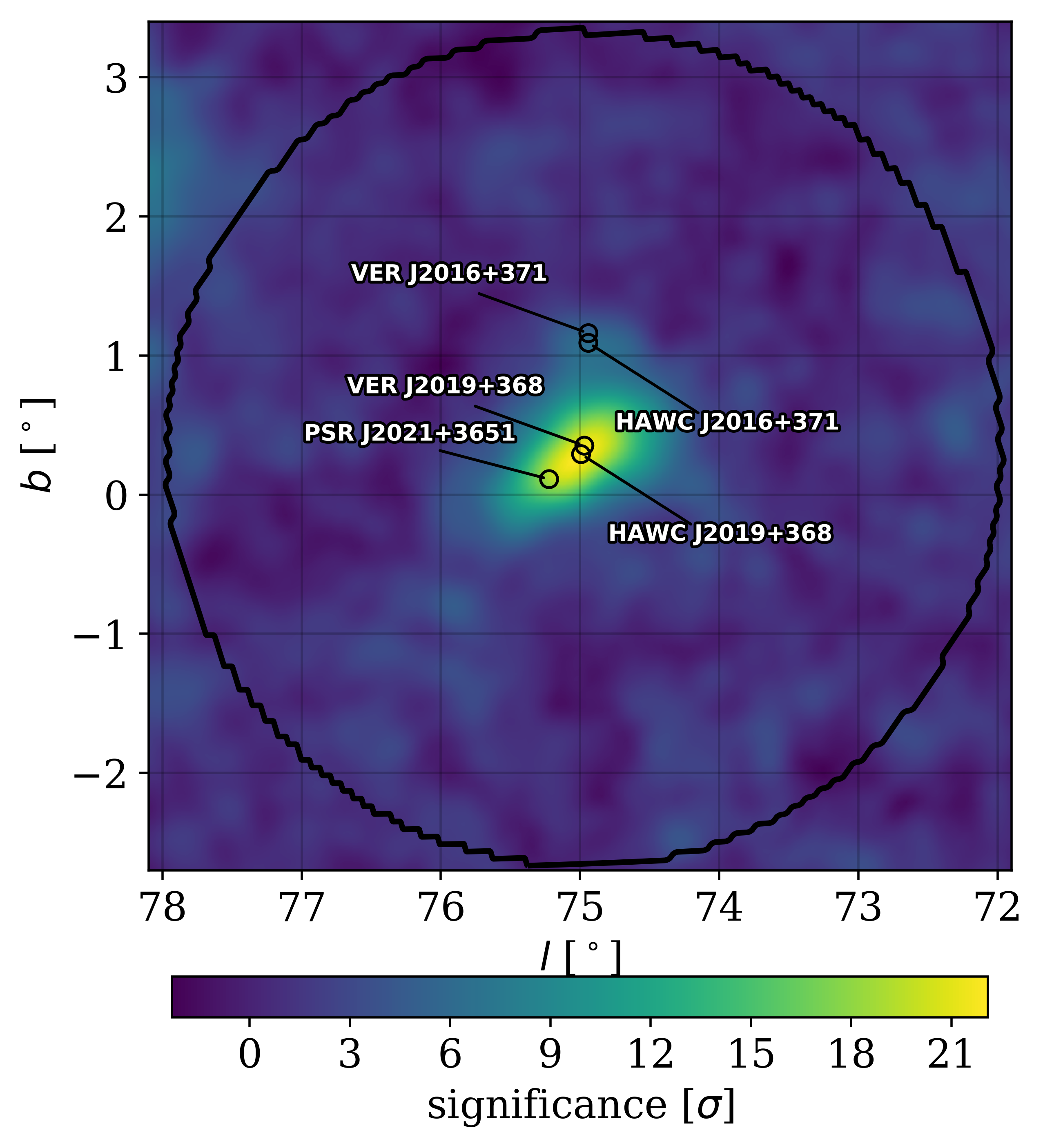
Figure 1: Significance map with relevant sources labelled assuming an $\alpha=-2.7$ spectrum. The ROI is indicated by the black circular contour. VERITAS source positions are taken from Abeysekara et al. (2018). The position of PSR J2021+3651 is taken from Roberts et al. (2002).

3 Morphological and Spectral Fit

As shown in Figure 1, this region is dominated by emission near the center of the ROI. The best-fit model is comprised of two sources: HAWC J2019+368 and HAWC J2016+371 on top of a uniform background. The background accounts for emission from extended sources potentially leaking into the ROI, such as one or more extended or diffuse $\gamma$-ray sources. At first, when considering a single source morphological hypothesis, a significant excess was seen nearly coincident with VER J2016+371. Adding a point source, HAWC J2016+371, at the location of the maximum residual improved the model by $\Delta\mathrm{TS}=39.0$. The need for a second source is also clear from Figure 2, where a $5\sigma$ excess is visible at the location of VER J2016+371.

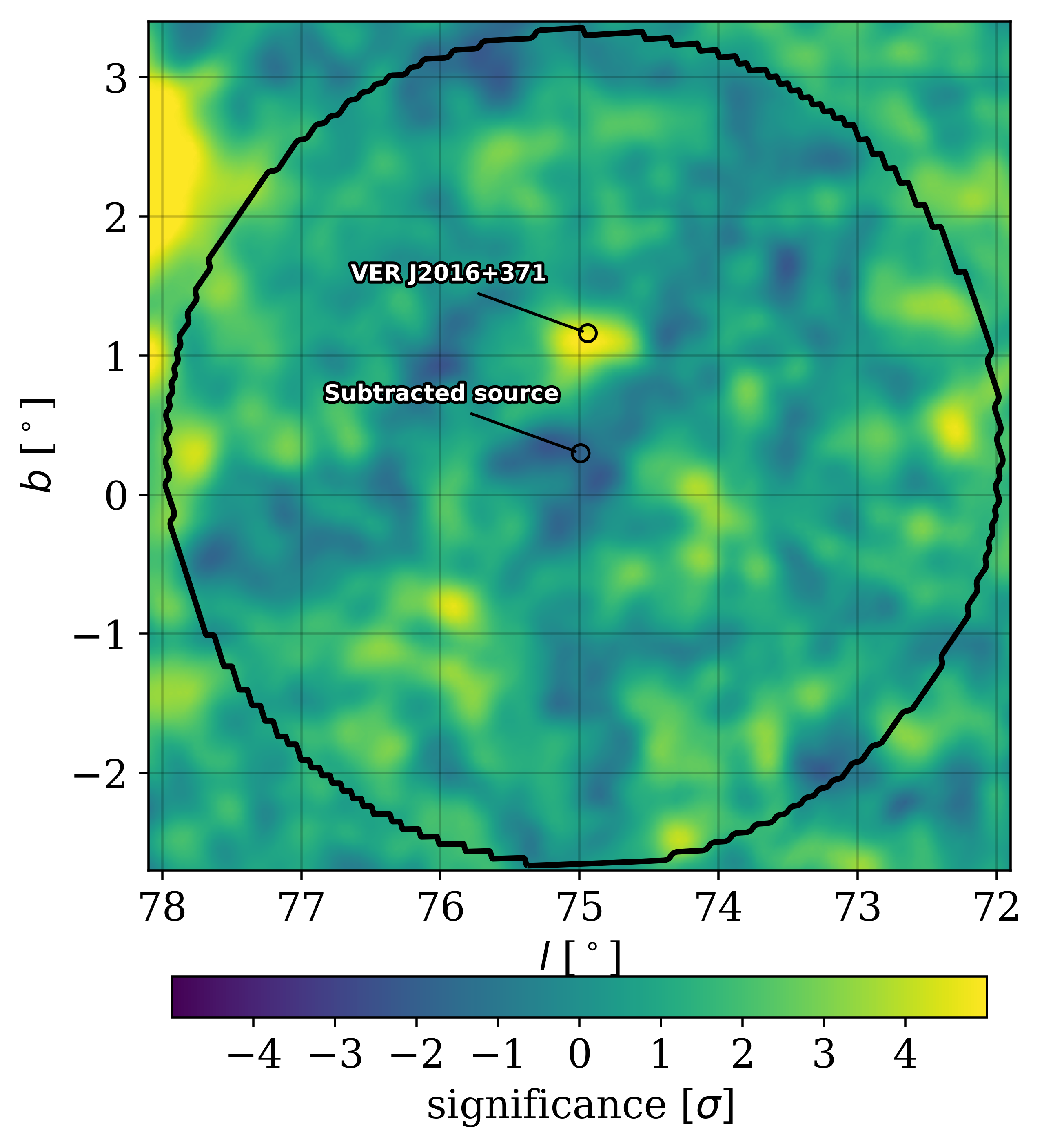
Figure 2: Analysis region with a single source subtracted (corresponding to modeling HAWC J2019+368 as an elliptical Gaussian with a power law spectrum). The maximum significance in the ROI is $\sqrt{\rm{TS}}=5.1$. This new source is called HAWC J2016+371.

Then, including a uniform background source improved the model consisting of HAWC J2019+368 and HAWC J2016+371 by $\Delta\mathrm{TS}=29.3$. This model, consisting of two $\gamma$-ray sources and a background, is then taken as the nominal source model of the region. HAWC J2019+368 and HAWC J2016+371 are located at (RA, Dec) = (304.92°, 36.76°) and (RA, Dec) = (304.1°, 37.2°), respectively. The model for HAWC J2019+268 is an elliptical gaussian shape, with parameters for the semimajor axis ($\mathrm{a}$), eccentricity ($\mathrm{e}$), and rotation describing the angle between the line of constant declination and the major axis ($\theta_{\rm{rot}}$). The model corresponds to an ellipse with minor axis $0.12\arcdeg\pm 0.02\arcdeg$. The pointing uncertainty on the source positions is $0.10\arcdeg$ (Abeysekara et al., 2017b).

Source Name	Spectral Parameters	Morphology
HAWC J2019+368	$\phi_{10\,\mathrm{TeV}}=4.05\pm 0.26\times 10^{-14}$ $\alpha=-2.02\pm 0.06$ $\beta=-0.29\pm 0.05$	$\mathrm{a}=0.368\arcdeg\pm 0.021$° $\mathrm{e}=0.943\pm 0.017$ $\theta_{\rm{rot}}=21.7\arcdeg\pm 2.5\arcdeg$
HAWC J2016+371	$\phi_{10\,\mathrm{TeV}}=2.6^{+0.7}_{-0.5}\times 10^{-15}$ $\alpha=-2.32\pm 0.18$	Point Source
Background	$\phi_{10\,\mathrm{TeV}}=8.2^{+1.5}_{-1.3}\times 10^{-14}$ $\alpha=-2.75\pm 0.08$	Uniform over ROI

Table 1: Description of model parameters assuming HAWC J2019+368 has a log parabolic spectrum. $\phi_{10\,\mathrm{TeV}}$ is the flux normalization at 10 TeV in units of $\mathrm{TeV}^{-1}\,\mathrm{cm}^{-2}\,\mathrm{s}^{-1}$. Reported uncertainties are statistical.

Source Name	Spectral Parameters	Morphology
HAWC J2019+368	$\phi_{10\,\mathrm{TeV}}=4.8^{+0.5}_{-0.4}\times 10^{-14}$ $\alpha=-1.67\pm 0.10$ $E_{\rm{cut}}=37^{+8}_{-7}$ TeV	$\mathrm{a}=0.358\arcdeg\pm 0.022$° $\mathrm{e}=0.953\pm 0.017$ $\theta_{\rm{rot}}=21.9\arcdeg\pm 2.6\arcdeg$
HAWC J2016+371	$\phi_{10\,\mathrm{TeV}}=2.9^{+0.7}_{-0.6}\times 10^{-15}$ $\alpha=-2.28\pm 0.17$	Point Source
Background	$\phi_{10\,\mathrm{TeV}}=8.1^{+1.5}_{-1.3}\times 10^{-14}$ $\alpha=-2.74\pm 0.09$	Uniform over ROI

Table 2: Description of model parameters assuming HAWC J2019+368 has an exponentially cutoff power law spectrum. $\phi_{10\,\mathrm{TeV}}$ is the flux normalization at 10 TeV in units of $\mathrm{TeV}^{-1}\,\mathrm{cm}^{-2}\,\mathrm{s}^{-1}$. Reported uncertainties are statistical.

A study looking for curvature in the spectrum of HAWC J2019+368 is then performed. A log parabola (power law with exponential cutoff) spectral assumption for HAWC J2019+368 is significantly preferred over a pure power law model by $\Delta\mathrm{TS}=69.0$ ($58.9$). Using $\mathrm{BIC}$ to find the preferred model between the (non-nested) curved spectral models, a log parabola spectrum is preferred with a $\Delta\mathrm{BIC}=10.1$. The best fit parameters for the reported log parabola spectrum are shown in Table 1. The best fit parameters for an exponentially cutoff power law are shown in Table 2. The spectral energy distribution of HAWC J2019+368 is shown in Figure 3, with the VERITAS data points from Abeysekara et al. (2018) scaled by 2.7 according to the procedure described in Section 3.1. The HAWC J2016+371 spectral energy distribution is shown in Figure 4, with the corresponding data points from Abeysekara et al. (2018). HAWC J2016+371 was not significantly detected in any individual energy bin, and therefore only the fit is reported here.

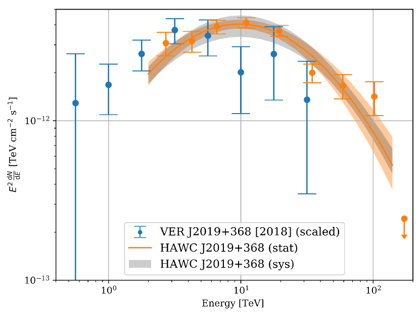
Figure 3: Spectral energy distribution of HAWC J2019+368. VERITAS data points are taken from Abeysekara et al. (2018) after the scaling detailed in Section 3.1. Upper limits are reported for energy bins whose $TS$ is less than 4.

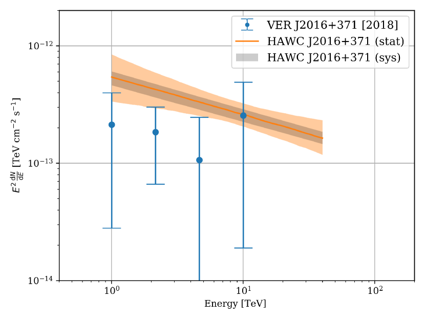
Figure 4: Spectral energy distribution of HAWC J2016+371. VERITAS data points are taken from Abeysekara et al. (2018). No scaling of VERITAS data points was performed as discussed in Section 3.1.

The systematic uncertainty bands shown in Figures 3 and 4 are produced by fitting the best model described above while varying the simulated model of HAWC. The same procedure and detector response files were used to produce the systematic uncertainty band as in Abeysekara et al. (2019). The plotted energy range is determined by adding a step function cutoff to the nominal model, and stopping when the $\Delta\mathrm{TS}$ equals one between the nominal model and the nominal model with the cutoff. This procedure is done twice —once at the higher energies and once at the lower energies— to determine the energy range over which this model describes the source.

3.1 Comparison to VERITAS measurements

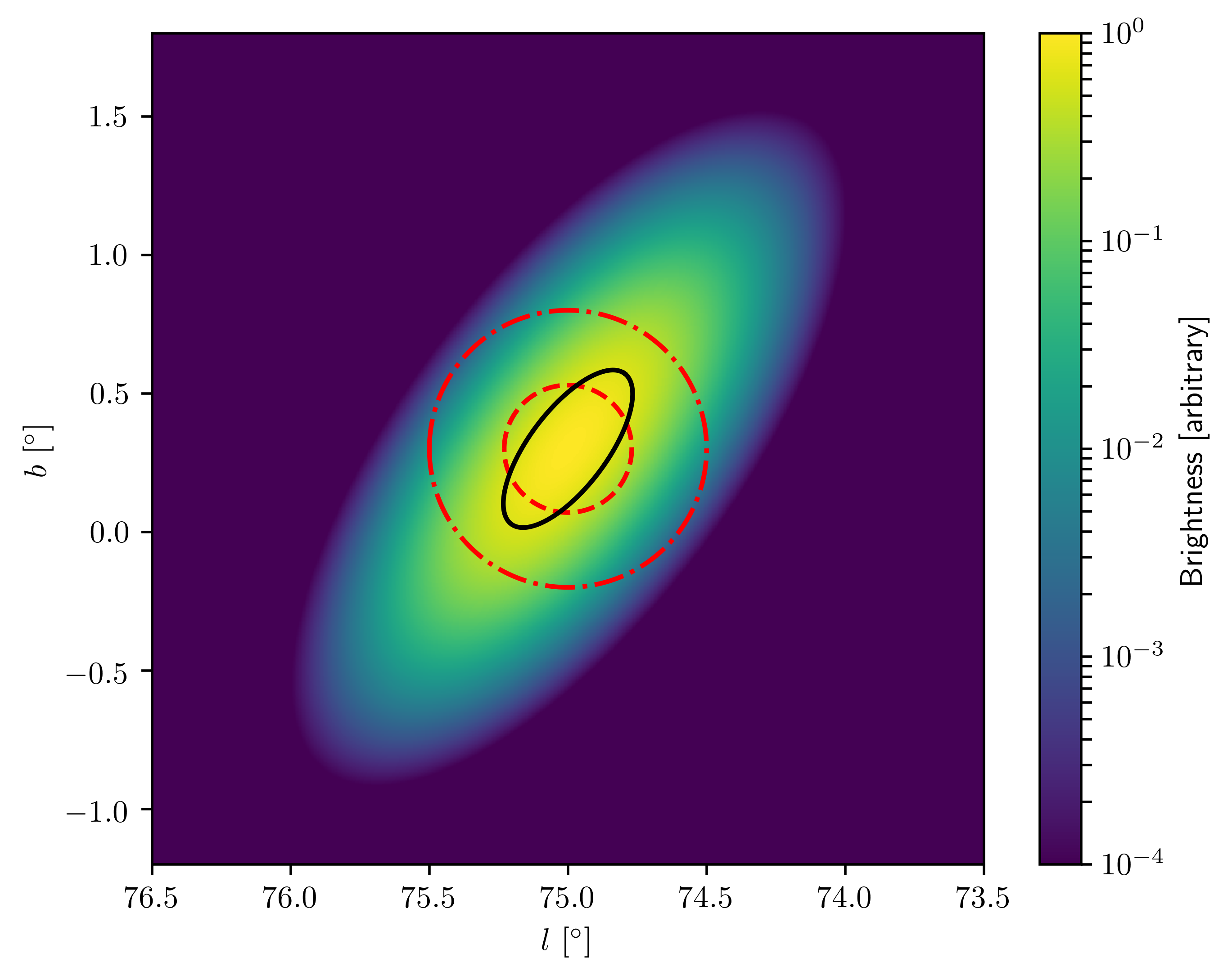
Figure 5: VERITAS Morphology map of VER J2019+368 (taken from Abeysekara et al. (2018)). The smaller red contour is the 0.23° extraction region from which the spectrum reported in Abeysekara et al. (2018) is taken. The larger red dashed contour is the 0.5° from which the spectrum reported in Aliu et al. (2014) is taken. The black elliptical contour is the 1$\sigma$ contour for the morphology reported in this work for HAWC J2019+368. The color scale is arbitrary and scaled such that the maximal pixel value is 1.

From their studies published in 2014 and 2018, the VERITAS collaboration extracted a spectrum from a smaller region than the reported morphology of the source (Aliu et al., 2014; Abeysekara et al., 2018). This is different from HAWC, where the morphology and spectrum are fit simultaneously in the ROI. This leads to a predictable systematic offset in the reported flux between the two instruments when two conditions are met: the measured morphology by VERITAS is larger than the extraction region, and the morphologies measured by HAWC and VERITAS are similar. This is not as significant an issue for sources that appear point-like for both instruments such as VER J2016+371 (Abeysekara et al., 2018) and HAWC J2016+371 (this work) or the Crab Nebula (Abeysekara et al., 2019; Meagher, 2015).

To account for this, we divide the flux reported by VERITAS by the fraction of the reported morphology contained within the extraction region. This has the effect of scaling the flux up to the morphology by a factor of $2.71$, under the assumption that the spectrum is the same for the entire source extent. In Figure 5 one can see that a substantial fraction of the source reported in Aliu et al. (2014) and Abeysekara et al. (2018) is not contained by the extraction region used to report the spectrum.

4 Energy Dependent morphology

To study the potential energy-dependent morphology of HAWC J2019+368, we examine the longitudinal profile of the data. The profile of the excess counts over the background is obtained within a region of the sky in different energy bands. The quarter decade energy bins were combined into four energy bands from 0.3-1.7 TeV, 1.7-10 TeV, 10-56 TeV, and 56-316 TeV to perform the study. A selection of the 2D bins ( as described in Abeysekara et al. (2019)) is done in each energy band (fraction hit bins greater than 2, 5, 7, and 9 for the energy bands 1, 2, 3, and 4, respectively) so that the best Point Spread Function (PSF) possible is retained without significantly losing statistics in each bin.

The region taken for the profiles is centered at the location of the PSR J2021+3651. The orientation of the region is along the position angle of $-77.90$°, which is the line joining the PSR J2021+3651 and HAWC J2019+368 positions. This orientation was chosen to test the hypothesis that the peak of the TeV emission would move to the pulsar location with increasing energy together with the change in the size of the emission region.

The profiles are 0.7°$\times$ 6° on the sky with 50 bins in the four reconstructed energy bands and are shown in the left panel of Figure 6.

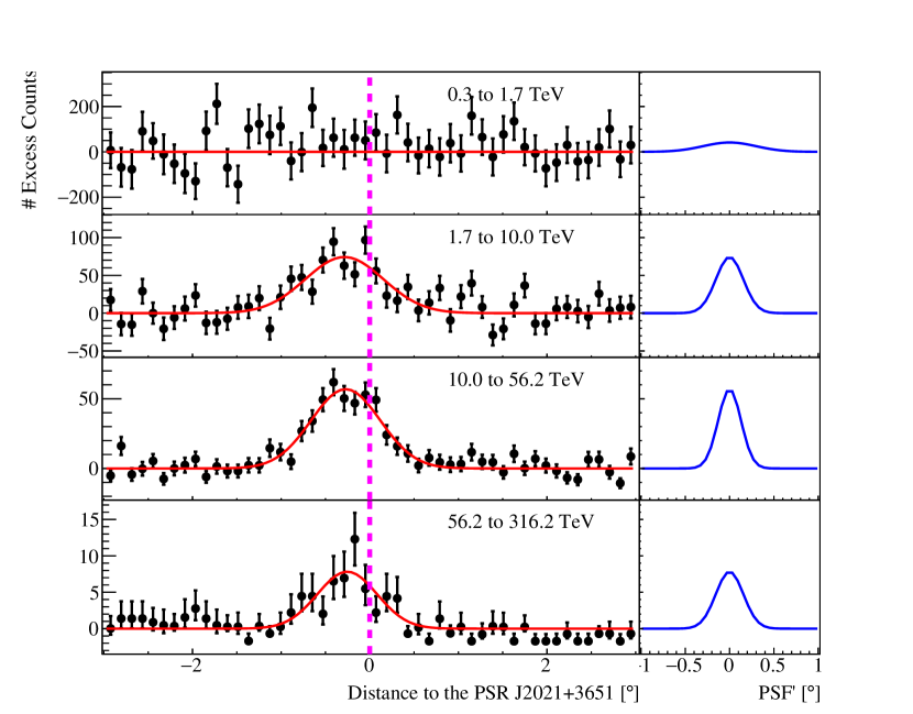
Figure 6: The longitudinal profiles of the excess counts maps for HAWC J2019+368 in different energy bands. The corresponding PSF^′ is shown on the right of each plot in blue (see Section 4). The profiles are fitted with a Gaussian shown in red. The location of the pulsar PSR J2021+3651 is shown with the magenta dashed line.

The width (0.7°) was chosen to avoid possible contamination from HAWC J2016+371 in the region of HAWC J2019+368. There was no significant emission observed in the first energy band, which might be due to the hard spectrum of HAWC J2019+368. The measured spectrum for HAWC J2019+368 also shows that the first significant flux point is at $>2$ TeV (see Figure 3), which is in agreement with the upper bound of the first energy band at 1.77 TeV. We see significant excess in energy bands 2, 3, and 4, which corresponds to the energy range above 1.77 TeV. The excess profiles were fitted with a Gaussian function and examined for size and location of the centroid of emission relative to PSR J2021+3651.

To estimate the size of the PSF in each longitudinal profile, we simulated a point source at the location of PSR J2021+3651 with a power law of spectral index 2.2. Similarly, excess count profiles are obtained and fitted with a Gaussian for this simulated point source. This $1\sigma$ width of the fitted Gaussian is hereafter referred to as PSF^′ for the purposes of this study. The PSF^′ obtained for different energy bands are shown in the right panel of Figure 6.

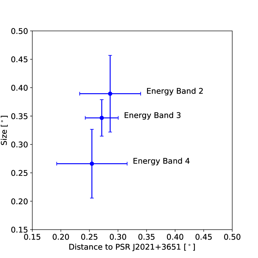
Figure 7: The size vs. distance with respect to the pulsar PSR J2021+3651 in different energy bands for HAWC J2019+368. Size is defined as the $\sqrt{\sigma_{\rm Fit}^{2}-(\sigma_{\rm PSF^{\prime}}+0.05)^{2}}$, where $\sigma_{\rm Fit}$ and $\sigma_{\rm PSF^{\prime}}$ is the $1\sigma$ width of the fitted Gaussian as shown in Figure 6. The PSF^′ is corrected for the systematic difference of 0.05^∘ between data and simulations (see Section 4). The mean position of the fitted Gaussian is used to calculate the distance to the pulsar location.

In Figure 7 we show the size and distance of the peak TeV emission with respect to the pulsar location in energy bands 2, 3, and 4 using the excess count profiles. The size was obtained by subtracting the $1\sigma$ width of the PSF^′ in quadrature from the $1\sigma$ fit size of the excess profiles in each energy band. The $1\sigma$ width of the PSF^′ was corrected by $0.05^{\circ}$ to account for a systematic difference of 5% between simulations and data (Abeysekara et al., 2019). The distance to the pulsar was calculated from the mean position of the excess profile fit. There is a very mild indication of the decrease in size with energy bands of increasing energy. However, the uncertainty on the measured size is large and there is no significant shift towards the pulsar position with increasing energy.

5 Spectral Modeling

Amongst the different scenarios that can explain the multi-wavelength emission from HAWC J2019+368, the observed spatial association between the X-ray and TeV emission, as well as the mild indication that the size of the TeV emission shrinks with increasing energy, seem to point towards a leptonic origin. Therefore we limit this analysis to a leptonic scenario. Exploring a hadronic or a lepto-hadronic origin of the TeV emission and their comparison is beyond the scope of this work.

In this section, we present a model assuming a leptonic scenario where the emission is originated by a PWN powered by PSR J2021+3651. The observed period ($P$) and its time derivative ($\dot{P}$) are 104 ms and $9.57\times 10^{-14}$ s s^-1, respectively, for PSR J2021+3651 (Roberts et al., 2002). The characteristic age, $\tau_{c}$, of the pulsar is 17.2 kyr (see Equation 1). It is worthwhile to note that the $\tau_{c}$ is only an accurate measure of the pulsar age,

$$\tau=\frac{P}{(n-1)\dot{P}}\left[1-\left(\frac{P_{0}}{P}\right)^{n-1}\right],$$ (1)

when the assumption of braking index $n=3$ and the birth period $P_{0}\ll P$ is true (Gaensler & Slane, 2006). For the distance to the pulsar, the dispersion-based measurement is quite large, $\geq$ 10 kpc (Roberts et al., 2002), which conflicts with distance derived considering the X-ray measurements (Van Etten et al., 2008) of $\sim 4$ kpc. The recent study of Chandra archival X-ray data by Kirichenko et al. (2015), taking into account an extinction-distance relation using the red-clump stars as standard candles in the line of sight, suggests a distance of $\sim\!\!1.8$ kpc. Therefore in this work, we will be using the distance of 1.8 kpc.

In the following, we will describe the model in Section 5.1 and then move to two scenarios where the model will be used to describe the observed X-ray and TeV emission together. In the first scenario, designated the one zone model (see Section 5.2), the observed X-ray and the whole range of TeV emission are described together. However, it is not ideal to model the X-ray emission between 2 and 10 keV (hard X-ray emission) together with TeV emission between $\sim\!\!1$ TeV and at least $\sim\!\!100$ TeV $\gamma$-ray energy because different components of the parent electron population (hereafter meaning both electrons and positrons) are responsible for the emission measured at X-ray and TeV energies. The size of the X-ray emission, $\sim\!\!4^{\prime}\times 10^{\prime}$ in full width at half maximum (Mizuno et al., 2017), is very small compared to the HAWC TeV emission of size $\sim\!\!20^{\prime}\times 50^{\prime}$ ($1\sigma$ containment, see Table 1). The component of the electron population emitting hard X-rays at 2-10 keV must be the one emitting the highest energy $\gamma$-rays at several tens of TeV and must be of higher energy than the one responsible for the extended TeV emission. This is because lower energy electrons have longer cooling timescales and can still produce TeV emission by traveling farther.

In the second scenario, the two zone model (see Section 5.3), the X-ray emission is compared with the highest energy TeV emission. Only the recently injected electrons will be used to describe the X-ray emission together with the whole history of injected electrons to describe the TeV emission. The possibility of undetected X-ray emission, comparable to the size of the TeV emission region will be taken into account to describe the whole history of the system.

5.1 Model Considerations

The pulsar braking index is assumed to be $n=3$. The cut-off energy ($E_{\rm max}$), the birth period ($P_{0}$), and the conversion efficiency ($\epsilon$) are treated as unknown parameters to describe the injected particle spectrum. The true age ($\tau$) of the system is calculated as a function of $P_{0}$ using Equation 1 instead of using the characteristic age ($\tau_{c}$).

We used the GAMERA software to perform the spectral modelling (Hahn, 2016). GAMERA can define a time-dependent model of relativistic electrons, including injection and cooling, and output the associated photon emission given a set of radiation fields. We consider a broken power-law with an exponential cut-off for the spectrum of the injected electrons. The break in the injected electron spectrum is believed to be due to two different electron populations (wind and radio) which dominate below and above the break energy ($E_{b}$) respectively. The value of $E_{b}$ and the injection spectral indices of the radio and wind populations are set to be their typical values of 0.1 TeV, $-1.5$, and $-2.0$ (Meyer et al., 2010; Atoyan & Aharonian, 1996). A cut-off is treated as a free parameter because the injected particles (e^±) can only be accelerated up to a certain maximum energy ($E_{\rm max}$) (Zhang et al., 2008; Gaensler & Slane, 2006). The radiation fields used to calculate the IC emission are calculated from the model presented in Popescu et al. (2017) at the location of PSR J2021+3651.

The time evolution of the parameters $B$, $\dot{E}$, and $P$ are specified following Gaensler & Slane (2006). The spin-down time scale ($\tau_{0}$) of the system is an important input for defining the time evolution of electrons in the system (Gaensler & Slane, 2006; Venter & de Jager, 2007). The spin-down timescale can be expressed as a function of $P_{0}$ as $\tau_{0}=P_{0}^{2}P^{-1}/{(2\dot{P})}$ (Gaensler & Slane, 2006). This allows us to choose the birth period of the pulsar that gives the best fit to the data. The nebular B-field is given by $B(t)={B_{0}}[1+(t/\tau_{0})^{0.5}]^{-1}$. The normalization of the injected particle spectrum is determined by $\epsilon\times\dot{E}(t)$, the fraction of the spin-down luminosity going into the production of electrons. The function $\dot{E}(t)$ is defined as $\dot{E}(t)=\dot{E}_{0}\left(1+t/\tau_{0}\right)^{-2}$. Lastly, the pulsar slows down its rotation according to $P(t)=P_{0}\left(1+t/{\tau_{0}}\right)^{0.5}$.

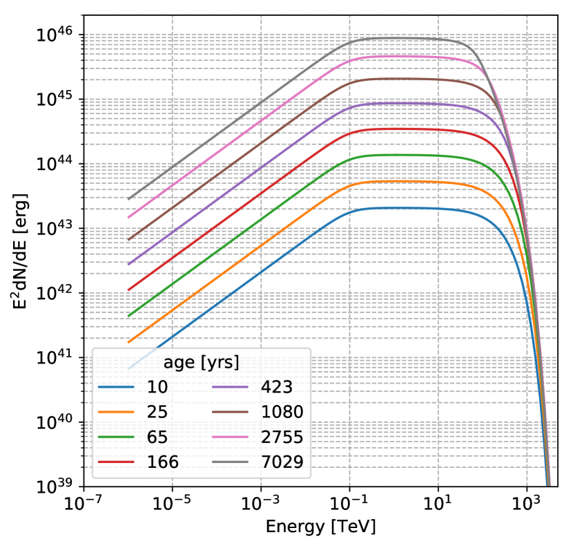
Figure 8: Time evolution of the particle e^± spectrum for the two-zone model described in Section 5.3. Ages are equal steps of 0.2 $\log_{10}(t$ years${}^{-1})$.

This way, our data constrains the birth period and also estimates the true age of the system. The injected particle spectrum for given values of assumed and unknown parameters is then evolved in the presence of magnetic and radiation fields to calculate the evolved particle spectrum as shown in Figure 8. The evolved particle spectrum is used to calculate the emitted photon spectrum, which is then matched to the observed X-ray and TeV emission.

5.2 One Zone Model

The emitted photon spectrum of the one zone model is shown in Figure 9. The model synchrotron (dashed lines) and IC (solid lines) emission are manually tuned to match the observed X-ray and $\gamma$-ray emission. It can be seen that the model synchrotron and IC emission are reasonably consistent with the observed X-ray and $\gamma$-ray data SED.

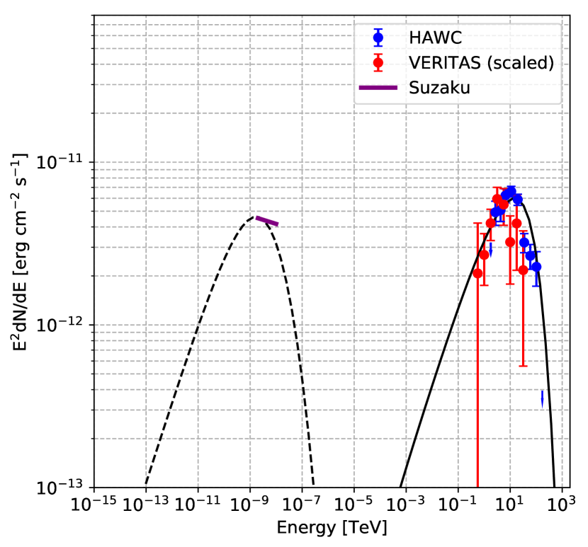
Figure 9: One zone model SED for synchrotron and IC are shown with dashed and solid lines respectively. The X-ray SED obtained by Suzaku and $\gamma$-ray SEDs for HAWC and VERITAS are shown (same as in Figure 3). The model SED is tuned manually to provide an approximate match to the X-ray and $\gamma$-ray emission in the whole energy range. The present-day B-field is 2 $\,\mu$G

The estimated value of the present day magnetic field is 2 $\mu$G, which is low (relative to the ISM) and depends on the relative normalization of the peak of the synchrotron and IC emission. The estimated value for $P_{0}$ of $80$ ms corresponds to an age of $\sim$7 kyr for the system. The required conversion efficiency ($\epsilon$) of pulsar spin-down power to particle injection is $5\%$, with the estimated cut-off energy ($E_{\rm max}$) of the injected particle spectrum being 300 TeV. However, there are certain limitations of the outcomes of the one zone model mainly pertaining to the obtained B-field of 2 $\mu$G. The estimated value of the B-field is very low in comparison to all expectations for a PWN and to the mean B-field of the local ISM ($\sim 3\mu$G). This model would predict identical X-ray and $\gamma$-ray morphology, which is in contradiction with the observations, as the observed size of the X-ray PWN is significantly smaller than that of the TeV emission.

5.3 Two Zone Model

The low magnetic field derived in the one-zone model indicates that describing the TeV and hard X-ray (2-10 keV) emission together using the whole electron population is not optimal. The limitations of the one zone model can be resolved by considering that the electrons producing hard X-rays are only a subset of the total electron population emitting $\gamma$-rays. The energy of an electron ($E_{e}$, as given in Mizuno et al. (2017)), emitting synchrotron radiation with mean energy $E_{\rm X-ray}$, due to a magnetic field $B$, is given by

$$E_{e}\simeq 132\text{TeV}\left(\frac{E_{\rm X-ray}}{\text{1keV}}\right)^{0.5}\left(\frac{B}{3\mu{\rm G}}\right)^{-0.5}.$$ (2)

Assuming a minimum magnetic field strength of 3$\,\mu$G (equal to the local ISM) the corresponding parent electron population component should be of energy $\sim$300 TeV for 5 keV X-rays (Mizuno et al., 2017).

Given the radiation fields from the model at 300 TeV electron energies, the most relevant radiation field is the Cosmic Microwave Background (CMB), with a magnetic field strength of $\sim$3$\,\mu$G. The relevant cooling timescales are of the order of $\sim$2 kyr using

$$\tau_{\rm cool}\approx 3.1\times 10^{5}\left(\frac{U}{\text{eV}\text{cm}^{-3}}\right)^{-1}\left(\frac{E_{e}}{\text{TeV}}\right)^{-1}\text{yr},$$ (3)

where the total energy density, $U$m is defined as $U=f_{\rm KN}U_{\rm ph}+0.025(B/{\mu}{\rm G})^{2}$ eV cm^-3 with respect the radiation field energy density $U_{\rm ph}$), the magnetic field ($B$), and $f_{\rm KN}$, the normalization factor to take into the suppression of IC losses due to KN effects (Hinton & Hofmann, 2009). The normalization factor can be calculated as:

$$f_{\rm KN}\approx\left(1+15\frac{E_{e}}{\text{TeV}}\frac{E_{T}}{\text{eV}}\right)^{-1.5},$$ (4)

where $E_{T}$ is the target photon energy (Hinton & Hofmann, 2009). We manually tune the B-field to match the observed normalization of X-ray emission such that the electrons currently producing hard X-rays are as much as 2 kyr old, resulting in a required present day B-field of 3.5 $\mu$G.

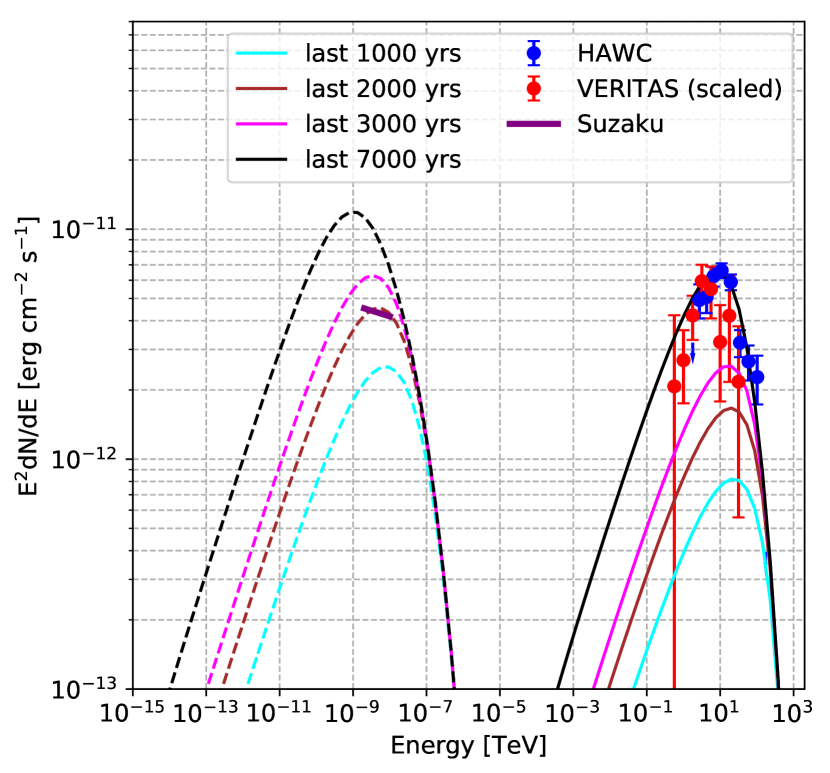
Figure 10: Two-zone model SED for synchrotron and IC are shown with dashed and solid lines, respectively. Model SEDs due to electron population injected in last 1, 2, and 3 kyr are also drawn together with the total time-integrated emission. The X-ray SED obtained by Suzaku (Mizuno et al., 2017) and $\gamma$-ray SEDs for HAWC and VERITAS are shown (same as in Figure 3). The model SED is tuned manually to provide an approximate match to the X-ray emission by electron population injected in last 2 kyr, and TeV emission in the whole energy range by the total injection history ($\sim$7 kyr). The required present-day B-field is 3.5 $\mu$G.

To match the model synchrotron and IC peak to the observed X-ray and TeV emission peak, a birth period of 80 ms is required, therefore the true age of the system for the two-zone model agrees with the one-zone model with a value of $\sim$7 kyr. However, due to the increased B-field, the conversion efficiency is marginally increased to a value of 6.5% in this case. The cut-off energy in the injected particle spectrum remains the same.

In Figure 10, the model SED lines for electrons injected in the last 1, 2 and 3 kyr are shown together with the total injection history of $\sim$7 kyr. In this case, the total synchrotron emission overshoots the observed X-ray SED by a factor of 4-5 at 2 keV. This may be due to the smaller region on the sky observed by the X-ray observations compared to the TeV observations, and result in some of the emission being unmeasured. It is also mentioned by Mizuno et al. (2017) that the observed X-ray emission should be taken as the lower limit.

The X-ray emission seen by Suzaku is $\sim\!\!4^{\prime}\times 10^{\prime}$ in full width at half maximum (Mizuno et al., 2017) while the $\gamma$-ray emission is about $\sim\!\!20^{\prime}\times 50^{\prime}$ using the same measure, meaning the TeV emission seen by HAWC is a factor of 25 larger in solid angle compared to the Suzaku observations. The dimmest reported flux from the Suzaku observations is $\sim\!\!1.7\times 10^{-13}$ erg cm^-2 s^-1 in a $5^{\prime}\times 3^{\prime}$ region (Mizuno et al., 2017). By scaling this flux in X-rays from the smaller observed region to the HAWC emission region, one would get a factor of 2-3 higher in measured X-ray flux.

The peak of the X-ray SED at 2 keV is about $\sim\!\!4\times 10^{-12}$ erg cm^-2 s^-1, therefore by taking into account the expected missing emission it would be around $\sim\!\!1\times 10^{-11}$ erg cm^-2 s^-1. On Figure 10 the present day synchrotron peak is near the value of $\sim\!\!10^{-11}$ erg cm^-2 s^-1, whereas the observed peak is coincides with the most recent $\sim\!\!2$ kyr of emission. The observed $\gamma$-ray emission can be compared to the model emission, where it can be seen that the model’s present-day IC emission is reasonably consistent with the observed TeV emission.

6 Discussion

To examine the obtained birth period ($P_{0}$) of 80 ms and true age ($\tau$) of $\sim\!\!7$ kyr, one can compare HAWC J2019+368 with the observed behaviour of HESS J1825-137. Both of these sources are bright extended TeV sources with similar associated pulsars. The associated pulsar of HESS J1825-137 is PSR B1823-13. The comparison of the pulsar properties of PSR J2021-3651 and PSR B1823-13 is shown in Table 3.

Source	HAWC J2019+368	HESS J1825-137
Associated pulsar	PSR J2021+3651	PSR B1823-13
Present period ($P$)	104 ms	102 ms
$\dot{P}$	$9.57\times 10^{-14}$ s s-1	$7.5\times 10^{-14}$ s s-1
$\dot{E}$	$3.4\times 10^{36}$ erg s-1	$2.8\times 10^{36}$ erg s-1
Characteristic Age ($\tau_{c}$)	17.2 kyr	21.4 kyr
Distance ($d$)	1.8 kpc	4 kpc

Table 3: Comparison of the associated pulsar properties of HAWC J2019+368 and HESS J1825-137 (Manchester et al., 2005; Roberts et al., 2002; Kirichenko et al., 2015).

It can be seen that both pulsars have similar $P$, $\dot{P}$, $\dot{E}$, and $\tau_{c}$. However, the main difference lies in the observed $\gamma$-ray luminosities of these two systems. For a given distance of 1.8 kpc and 4 kpc for HAWC J2019+368 and HESS J1825-137, respectively, the integrated $\gamma$-ray luminosities are $\sim\!\!10^{33}$ and $\sim\!\!10^{35}$ erg s^-1, respectively. In order to match the $\gamma$-ray luminosity of HAWC J2019+368 to the one for HESS J1825-137, the distance to the HAWC J2019+368 system would have to be $\sim\!\!18$ kpc. However, with the previous distance measurements this seems to be very unlikely (see Section 5.1). In both systems, the assumed conversion efficiency of spin-down power of the pulsar to e^± are below 10% (Aharonian et al., 2006). Assuming the radiation fields in both systems do not differ drastically, and with similar B-fields of a few $\mu$G, the energy conversion efficiency of e^± to $\gamma$-ray production should be similar for both. One possible explanation for the differing luminosities is that PSR J2021+3651 has a larger $P_{0}$ (80 ms in this work) compared to PSR B1823-13 ($\sim$1 ms or $\sim$15 ms, from Khangulyan et al. (2018); Principe et al. (2020)). Due to the similar present day $P$ and $\dot{P}$ of the two systems and assuming $\dot{P}$ did not change rapidly in the past, PSR B1823-13 must have injected more power into the system compared to PSR J2021+3651.

The larger $P_{0}$ of PSR J2021+3651, in turn, makes the HAWC J2019+368 system younger ($\sim$7 kyr) compared to its characteristic age of $\sim$17 kyr. This interpretation agrees with the peak emission energies of HESS J1825-137 and HAWC J2019+368, which are at $\sim\!\!0.1$ TeV (Principe et al., 2020) and $\sim\!\!20$ TeV (Figure 3), respectively. Given the pulsars’ observed similarity, the pulsar powering HAWC J2019+368 system should be younger than the one powering HESS J1825-137 to explain the different spectral features at TeV energies: the higher peak emission energy and hard spectrum below $\sim$20 TeV.

One can estimate the parent electron population energy for a given $\gamma$-ray photon energy in the Thompson regime (only assuming CMB, see Longair (2011)) as:

$$E_{e}\simeq 17.2\text{TeV}\left(\frac{E_{\gamma{\rm-ray}}}{1\text{TeV}}\right)^{0.5}.$$ (5)

For a 20 TeV photon, the parent electron population would be of energy $\sim$80 TeV. The KN effect only starts to dominate above tens of TeV of corresponding $\gamma$-ray energies (assuming electrons are only scattering off of CMB photons). Using equation 3, the corresponding cooling timescale for 80 TeV electrons in a 3.5 $\mu$G B-field and CMB are of the order of $\sim$9 kyr, which is similar to the estimated age of the system, $\sim$7 kyr. The electrons with energies $>80$ TeV are already cooled, making the TeV spectrum softer above $\gamma$-ray energies of $\sim$20 TeV. The lower-energy electron population $<80$ TeV has not cooled yet, making the spectral index hard up to 20 TeV in $\gamma$-ray energies. This can also be seen from Figure 8 where the break in the evolved particle spectrum can be seen at $\sim$80 TeV.

It is also to be noted that Aliu et al. (2014) showed cone-shaped radio emission starting at the pulsar location and extending towards the centroid of TeV emission for VER J2019+368. The positions of VER J2019+368 (RA, Dec = $304.846\arcdeg$, $36.779\arcdeg$) and HAWC J2019+368 (RA, Dec = $304.92\arcdeg$, $36.76\arcdeg$) are separated by $0.06\arcdeg$, which is within the VERITAS PSF (0.1° above 1 TeV) and HAWC PSF ($0.1$°-$0.3$° for the events above 3.16 TeV depending on the bin) (Aliu et al., 2014; Abeysekara et al., 2018, 2019). Both observations independently support the claim that emission at TeV energies is offset from the pulsar location (RA, Dec = $305.27275\arcdeg$, $36.85133\arcdeg$) by approximately $0.3\arcdeg$ (Abdo et al., 2009). This is because the lower energy ($<80$ TeV) electrons can still emit in TeV energies via IC due to their longer cooling timescales, and within that time the pulsar had moved to its present location. On the other hand, due to the higher energies of the X-ray emitting electrons and therefore smaller cooling timescales, the X-ray emission is closer to the pulsar position (Mizuno et al., 2017). If we assume that the pulsar was born at the location of HAWC J2019+368, and assume that the current location of the pulsar is due to only its proper motion, the transverse velocity would be $\sim$1300 km s^-1. The obtained transverse velocity is certainly at the higher end of the pulsar transverse velocity distribution (Faucher-Giguere & Kaspi, 2006), however it would not be unrealistic.

The measured extension of HAWC J2019+368 is about $0.36\arcdeg$ along the major axis obtained from the morphology fit using an asymmetric 2D Gaussian as described in Section 3, which would correspond to a projected size of $\sim$11 pc. In the energy-dependent morphology study (see Section 4), energy band 3 has similar size and corresponds to the energy range between 10 and 56 TeV. The median $\gamma$-ray energy in this band is $\sim$23 TeV, which corresponds to electron energy of about $\sim\!\!80$ TeV (using Equation 5).

Using these pieces of information, we may comment on the transport of electrons in an advection or diffusion scenario. Recalling that the cooling timescale of mono-energetic 80 TeV electrons is $\sim\!\!9$ kyr, the corresponding advective transport speed of electrons is about $\sim$1200 km s^-1. The Bohm diffusion coefficient is $D(E)=\eta r_{g}c/3$, where $r_{g}=3.3\times 10^{15}(E/10\rm{TeV})(B/10\mu{\rm G})^{-1}\rm{cm}$ and $c$ is the speed of light in vacuum (Aharonian, 2004). In the case of Bohm diffusion ($\eta=1)$, the diffusion coefficient in a 3.5 $\mu$G B-field would be $\sim\!\!7.5\times 10^{26}$ cm² s^-1. This value is similar to the case of Geminga and B0656+14 where the diffusion coefficient is much smaller than the ISM value derived from the boron-to-carbon ratio (Abeysekara et al., 2017c). The latter can be expressed as: $D(E)=D(10\rm{GeV})(E/10\rm{GeV})^{\delta}$, where $D(10\rm{GeV})\sim\!\!10^{28}$ cm² s^-1 and $\delta=0.5$ (Aharonian, 2004), which would yield a value of $\sim\!\!9\times 10^{29}$ cm² s^-1 for $\sim\!\!80$ TeV electrons.

If diffusion is the mechanism dominating the transport for HAWC J2019+368, it would imply that the magnetic field is much more turbulent than the average in the ISM, which is not surprising considering that we are in a region heavily dominated by the pulsar wind. Hence, the advection velocity or diffusion coefficient is constrained by the morphology of the TeV emission region. However, a detailed study of transport mechanisms (advection/diffusion) would require a better measurement of energy-dependent morphology.

7 Conclusions

In this work, we have performed the first detailed spectral and morphological study using HAWC data of the region surrounding MGRO J2019+37, resolving it into the sources HAWC J2019+368 and HAWC J2016+371. The morphology and spectrum in this work agrees well with the VERITAS measurements from Aliu et al. (2014) and Abeysekara et al. (2018), consisting of an elliptical Gaussian source (for HAWC J2019+368 and VER J2019+368) and point source (for HAWC J2016+371 and VER J2016+371). The agreement between HAWC and VERITAS for the spectrum and morphology in this region is an important milestone in comparisons between IACTs and ground array detectors like HAWC. Previously, differences between measured spectra and morphology were attributed to not well understood systematic differences (Abeysekara et al., 2017a). These differences may now be explainable and quantifiable (in some cases) as the difference between the extraction region used to produce the spectrum, and the morphology measured.

The detection of HAWC J2016+371 confirms the source VER J2016+371. Given its very recent confirmation as a PWN via X-ray measurements, as the HAWC exposure to this source grows, it may be useful to examine the emission from this source in detail to see if its TeV emission is similar to other PWNe, or if the supernova remnant hosting the nebula may be accelerating protons to TeV energies (Guest et al., 2020). Determining the origin of the uniform background $\gamma$-ray source in the morphology model is an important subject for future study.

We find that the emission from HAWC J2019+368 together with the X-ray data is well described via emission from a young PWN system powered by a $\sim$7 kyr old pulsar. This allows us to estimate the PWN properties of the system such as the magnetic field, the pulsar spin-down energy to electron conversion efficiency, and the maximum electron energy. Follow-up studies at X-ray energies may find a spatially extended emission region that might agree with the morphology measured by HAWC and VERITAS, a finding which would support the two zone model of electrons described in this work.

The energy-dependent morphology study does not show conclusive evidence in favor of shrinking size with increasing energy due to large uncertainties in the measurements. Nevertheless, it enables us to constrain the particle transport in a PWN system. This may be improved upon with more data in the future. The recent upgrade of HAWC with an outrigger array will play a crucial role by increasing HAWC’s sensitivity to showers at the highest energies as it increases the instrumented area of HAWC by a factor of 4-5 (Marandon et al., 2019; Joshi & Schoorlemmer, 2019).

8 Acknowledgements

We acknowledge the support from: the US National Science Foundation (NSF); the US Department of Energy Office of High-Energy Physics; the Laboratory Directed Research and Development (LDRD) program of Los Alamos National Laboratory; Consejo Nacional de Ciencia y Tecnología (CONACyT), México, grants 271051, 232656, 260378, 179588, 254964, 258865, 243290, 132197, A1-S-46288, A1-S-22784, cátedras 873, 1563, 341, 323, Red HAWC, México; DGAPA-UNAM grants IG101320, IN111315, IN111716-3, IN111419, IA102019, IN112218; VIEP-BUAP; PIFI 2012, 2013, PROFOCIE 2014, 2015; the University of Wisconsin Alumni Research Foundation; the Institute of Geophysics, Planetary Physics, and Signatures at Los Alamos National Laboratory; Polish Science Centre grant, DEC-2017/27/B/ST9/02272; Coordinación de la Investigación Científica de la Universidad Michoacana; Royal Society - Newton Advanced Fellowship 180385; Generalitat Valenciana, grant CIDEGENT/2018/034; Chulalongkorn University’s CUniverse (CUAASC) grant. Thanks to Scott Delay, Luciano Díaz and Eduardo Murrieta for technical support.

References

- Abdalla et al. (2019) Abdalla, H., Aharonian, F., Ait Benkhali, F., et al. 2019, Astron. Astrophys., 621, A116
- Abdo et al. (2007a) Abdo, A. A., Allen, B., Berley, D., et al. 2007a, Astrophys. J., 658, L33
- Abdo et al. (2007b) —. 2007b, Astrophys. J., 664, L91
- Abdo et al. (2009) Abdo, A. A., Ackermann, M., Ajello, M., et al. 2009, Astrophys. J., 700, 1059
- Abdo et al. (2012) Abdo, A. A., Abeysekara, U., Allen, B. T., et al. 2012, Astrophys. J., 753, 159
- Abeysekara et al. (2017a) Abeysekara, A. U., Albert, A., Alfaro, R., et al. 2017a, Astrophys. J., 843, 40
- Abeysekara et al. (2017b) —. 2017b, The Astrophysical Journal, 843, 39
- Abeysekara et al. (2017c) —. 2017c, Science (New York, N.Y.), 358, 911
- Abeysekara et al. (2018) Abeysekara, A. U., Archer, A., Aune, T., et al. 2018, Astrophys. J., 861, 134
- Abeysekara et al. (2019) Abeysekara, A. U., Albert, A., Alfaro, R., et al. 2019, The Astrophysical Journal, 881, 134
- Abeysekara et al. (2020) —. 2020, Physical Review Letters, 124, doi:10.1103/PhysRevLett.124.021102
- Aharonian et al. (2006) Aharonian, F., Akhperjanian, A. G., Bazer-Bachi, A. R., et al. 2006, Astron. Astrophys., 460, 365
- Aharonian (2004) Aharonian, F. A. 2004, Very high energy cosmic gamma radiation : a crucial window on the extreme Universe (World Scientific Publishing Co), doi:10.1142/4657
- Aliu et al. (2014) Aliu, E., Aune, T., Behera, B., et al. 2014, Astrophys. J., 788, 78
- Amenomori et al. (2008) Amenomori, M., Bi, X. J., Chen, D., & et al. 2008, International Cosmic Ray Conference, 2, 695
- Atoyan & Aharonian (1996) Atoyan, A. M., & Aharonian, F. A. 1996, MNRAS, 278, 525
- Bartko et al. (2008) Bartko, H., Benarek, W., Rico, J., & Saito, T. 2008, International Cosmic Ray Conference, 2, 649
- Bartoli et al. (2012) Bartoli, B., Bernardini, P., Bi, X. J., et al. 2012, ApJ, 745, L22
- Bednarek (2007) Bednarek, W. 2007, MNRAS, 382, 367
- Brisbois (2019) Brisbois, C. A. 2019, PhD thesis, Michigan Technological University. https://search.proquest.com/docview/2298170240?accountid=14696
- Faucher-Giguere & Kaspi (2006) Faucher-Giguere, C.-A., & Kaspi, V. M. 2006, Astrophys. J., 643, 332
- Gaensler & Slane (2006) Gaensler, B. M., & Slane, P. O. 2006, Annual Review of Astronomy and Astrophysics, 44, 17
- Guest et al. (2020) Guest, B., Safi-Harb, S., MacMaster, A., et al. 2020, Monthly Notices of the Royal Astronomical Society, 491, 3013
- Hahn (2016) Hahn, J. 2016, PoS, ICRC2015, 917
- Halpern et al. (2008) Halpern, J. P., Camilo, F., Giuliani, A., et al. 2008, ApJ, 688, L33
- Hessels et al. (2004) Hessels, J. W. T., Roberts, M. S. E., Ransom, S. M., et al. 2004, Astrophys. J., 612, 389
- Hinton & Hofmann (2009) Hinton, J. A., & Hofmann, W. 2009, Annual Review of Astronomy and Astrophysics, 47, 523
- Joshi (2019) Joshi, V. 2019, PhD thesis, U. Heidelberg (main), doi:10.11588/heidok.00026062
- Joshi & Schoorlemmer (2019) Joshi, V., & Schoorlemmer, H. 2019, in International Cosmic Ray Conference, Vol. 36, 36th International Cosmic Ray Conference (ICRC2019), 707
- Kass & Raftery (1995) Kass, R. E., & Raftery, A. E. 1995, Journal of the American Statistical Association, 773
- Khangulyan et al. (2018) Khangulyan, D., Koldoba, A. V., Ustyugova, G. V., Bogovalov, S. V., & Aharonian, F. 2018, Astrophys. J., 860, 59
- Kieda (2008) Kieda, D. B. 2008, International Cosmic Ray Conference, 2, 843
- Kirichenko et al. (2015) Kirichenko, A., Danilenko, A., Shternin, P., et al. 2015, Astrophys. J., 802, 17
- Liddle (2007) Liddle, A. R. 2007, Monthly Notices of the Royal Astronomical Society: Letters, 377, L74
- Longair (2011) Longair, M. S. 2011, High Energy Astrophysics (Cambridge University Press)
- Manchester et al. (2005) Manchester, R. N., Hobbs, G. B., Teoh, A., & Hobbs, M. 2005, AJ, 129, 1993
- Marandon et al. (2019) Marandon, V., Jardin-Blicq, A., & Schoorlemmer, H. 2019, arXiv e-prints, arXiv:1908.07634
- Meagher (2015) Meagher, K. 2015, ICRC (The Hague), 34, doi:10.22323/1.236.0792
- Meyer et al. (2010) Meyer, M., Horns, D., & Zechlin, H. S. 2010, A&A, 523, A2
- Mizuno et al. (2017) Mizuno, T., Tanaka, N., Takahashi, H., et al. 2017, Astrophys. J., 841, 104
- Moderksi et al. (2005) Moderksi, R., Sikora, M., Coppi, P. S., & Aharonian, F. A. 2005, Mon. Not. Roy. Astron. Soc., 364, 1488, [Mon. Not. Roy. Astron. Soc.363,no.3,954(2005)]
- Paredes et al. (2009) Paredes, J. M., Martí, J., Ishwara-Chandra, C. H., et al. 2009, Astron. Astrophys., 507, 241
- Popescu et al. (2017) Popescu, C. C., Yang, R., Tuffs, R. J., et al. 2017, MNRAS, 470, 2539
- Principe et al. (2020) Principe, G., Mitchell, A. M. W., Caroff, S., et al. 2020, arXiv e-prints, arXiv:2006.11177
- Roberts et al. (2002) Roberts, M. S. E., Hessels, J. W. T., Ransom, S. M., et al. 2002, Astrophys. J., 577, L19
- Saha & Bhattacharjee (2015) Saha, L., & Bhattacharjee, P. 2015, Journal of High Energy Astrophysics, 5, 9
- Sguera (2008) Sguera, V. 2008, in The 7th INTEGRAL Workshop, 82
- Van Etten et al. (2008) Van Etten, A., Romani, R. W., & Ng, C. 2008, Astrophys. J., 680, 1417
- Venter & de Jager (2007) Venter, C., & de Jager, O. C. 2007, in WE-Heraeus Seminar on Neutron Stars and Pulsars 40 years after the Discovery, ed. W. Becker & H. H. Huang, 40
- Vianello et al. (2018) Vianello, G., Riviere, C., Brisbois, C., Fleischhack, H., & Burgess, J. M. 2018, HAWC Accelerated Likelihood - python-only framework for HAWC data analysis, , . https://github.com/threeML/hawc_hal
- Vianello et al. (2015) Vianello, G., Lauer, R. J., Younk, P., et al. 2015, arXiv e-prints, arXiv:1507.08343
- Zhang et al. (2008) Zhang, L., Chen, S. B., & Fang, J. 2008, The Astrophysical Journal, 676, 1210