CADA: Communication-Adaptive Distributed Adam

Abstract

Stochastic gradient descent (SGD) has taken the stage as the primary workhorse for large-scale machine learning. It is often used with its adaptive variants such as AdaGrad, Adam, and AMSGrad. This paper proposes an adaptive stochastic gradient descent method for distributed machine learning, which can be viewed as the communication-adaptive counterpart of the celebrated Adam method — justifying its name CADA. The key components of CADA are a set of new rules tailored for adaptive stochastic gradients that can be implemented to save communication upload. The new algorithms adaptively reuse the stale Adam gradients, thus saving communication, and still have convergence rates comparable to original Adam. In numerical experiments, CADA achieves impressive empirical performance in terms of total communication round reduction.

1 Introduction

Stochastic gradient descent (SGD) method [Robbins and Monro(1951)] is prevalent in solving large-scale machine learning problems during the last decades. Although simple to use, the plain-vanilla SGD is often sensitive to the choice of hyper-parameters and sometimes suffer from the slow convergence. Among various efforts to improve SGD, adaptive methods such as AdaGrad [Duchi et al.(2011)Duchi, Hazan, and Singer], Adam [Kingma and Ba(2014)] and AMSGrad [Reddi et al.(2018)Reddi, Kale, and Kumar] have well-documented empirical performance, especially in training deep neural networks.

To achieve “adaptivity,” these algorithms adaptively adjust the update direction or tune the learning rate, or, the combination of both. While adaptive SGD methods have been mostly studied in the setting where data and computation are both centralized in a single node, their performance in the distributed learning setting is less understood. As this setting brings new challenges to machine learning, can we add an additional dimension of adaptivity to Adam in this regime?

In this context, we aim to develop a fully adaptive SGD algorithm tailored for the distributed learning. We consider the setting composed of a central server and a set of $M$ workers in ${\cal M}:=\{1,\ldots,M\}$, where each worker $m$ has its local data $\xi_{m}$ from a distribution $\Xi_{m}$. Workers may have different data distributions $\{\Xi_{m}\}$, and they collaboratively solve the following problem

$$\min_{\theta\in\mathbb{R}^{p}}~{}~{}~{}{\cal L}(\theta)=\frac{1}{M}\sum_{m\in{\cal M}}{\cal L}_{m}(\theta)~{}~{}~{}{\rm with}~{}~{}~{}{\cal L}_{m}(\theta):=\!\mathbb{E}_{\xi_{m}}\left[\ell(\theta;\xi_{m})\right],~{}m\in{\cal M}$$ (1)

where $\theta\in\mathbb{R}^{p}$ is the sought variable and $\{{\cal L}_{m},m\!\in\!{\cal M}\}$ are smooth (but not necessarily convex) functions. We focus on the setting where local data $\xi_{m}$ at each worker $m$ can not be uploaded to the server, and collaboration is needed through communication between the server and workers. This setting often emerges due to the data privacy concerns, e.g., federated learning [McMahan et al.(2017a)McMahan, Moore, Ramage, Hampson, and y Arcas, Kairouz et al.(2019)Kairouz, McMahan, Avent, Bellet, Bennis, Bhagoji, Bonawitz, Charles, Cormode, Cummings, et al.].

To solve (1), we can in principle apply the single-node version of the adaptive SGD methods such as Adam [Kingma and Ba(2014)]: At iteration $k$, the server broadcasts $\theta^{k}$ to all the workers; each worker $m$ computes $\nabla\ell(\theta^{k};\xi_{m}^{k})$ using a randomly selected sample or a minibatch of samples $\{\xi_{m}^{k}\}\sim\Xi_{m}$, and then uploads it to the server; and once receiving stochastic gradients from all workers, the server can simply use the aggregated stochastic gradient $\bar{\bm{\nabla}}^{k}=\frac{1}{M}\!\sum_{m\in{\cal M}}\nabla\ell(\theta^{k};\xi_{m}^{k})$ to update the parameter via the plain-vanilla single-node Adam. When $\nabla\ell(\theta^{k};\xi_{m}^{k})$ is an unbiased gradient of $\mathcal{L}_{m}(\theta)$, the convergence of this distributed implementation of Adam follows from the original ones [Reddi et al.(2018)Reddi, Kale, and Kumar, Chen et al.(2019)Chen, Liu, Sun, and Hong]. To implement this, however, all the workers have to upload the fresh $\{\nabla\ell(\theta^{k};\xi_{m}^{k})\}$ at each iteration. This prevents the efficient implementation of Adam in scenarios where the communication uplink and downlink are not symmetric, and communication especially upload from workers and the server is costly; e.g., cellular networks [Park et al.(2019)Park, Samarakoon, Bennis, and Debbah]. Therefore, our goal is to endow an additional dimension of adaptivity to Adam for solving the distributed problem (1). In short, on top of its adaptive learning rate and update direction, we want Adam to be communication-adaptive.

1.1 Related work

To put our work in context, we review prior contributions that we group in two categories.

1.1.1 SGD with adaptive gradients

A variety of SGD variants have been developed recently, including momentum and acceleration [Polyak(1964), Nesterov(1983), Ghadimi and Lan(2016)]. However, these methods are relatively sensitive to the hyper-parameters such as stepsizes, and require significant efforts on finding the optimal parameters.

Adaptive learning rate. One limitation of SGD is that it scales the gradient uniformly in all directions by a pre-determined constant or a sequence of constants (a.k.a. learning rates). This may lead to poor performance when the training data are sparse [Duchi et al.(2011)Duchi, Hazan, and Singer]. To address this issue, adaptive learning rate methods have been developed that scale the gradient in an entry-wise manner by using past gradients, which include AdaGrad [Duchi et al.(2011)Duchi, Hazan, and Singer, Ward et al.(2019)Ward, Wu, and Bottou], AdaDelta [Zeiler(2012)] and other variants [Li and Orabona(2019)]. This simple technique has improved the performance of SGD in some scenarios.

Adaptive SGD. Adaptive SGD methods achieve the best of both worlds, which update the search directions and the learning rates simultaneously using past gradients. Adam [Kingma and Ba(2014)] and AMSGrad [Reddi et al.(2018)Reddi, Kale, and Kumar] are the representative ones in this category. While these methods are simple-to-use, analyzing their convergence is challenging [Reddi et al.(2018)Reddi, Kale, and Kumar, Wang et al.(2020a)Wang, Lu, Tu, and Zhang]. Their convergence in the nonconvex setting has been settled only recently [Chen et al.(2019)Chen, Liu, Sun, and Hong, Défossez et al.(2020)Défossez, Bottou, Bach, and Usunier]. However, most adaptive SGD methods are studied in the single-node setting where data and computation are both centralized. Very recently, adaptive SGD has been studied in the shared memory setting [Xu et al.(2020)Xu, Sutcher-Shepard, Xu, and Chen], where data is still centralized and communication is not adaptive.

1.1.2 Communication-efficient distributed optimization

Popular communication-efficient distributed learning methods belong to two categories: c1) reduce the number of bits per communication round; and, c2) save the number of communication rounds.

For c1), methods are centered around the ideas of quantization and sparsification.
Reducing communication bits. Quantization has been successfully applied to distributed machine learning. The 1-bit and multi-bits quantization methods have been developed in [Seide et al.(2014)Seide, Fu, Droppo, Li, and Yu, Alistarh et al.(2017)Alistarh, Grubic, Li, Tomioka, and Vojnovic, Tang et al.(2018)Tang, Gan, Zhang, Zhang, and Liu]. More recently, signSGD with majority vote has been developed in [Bernstein et al.(2018)Bernstein, Wang, Azizzadenesheli, and Anandkumar]. Other advances of quantized gradient schemes include error compensation [Wu et al.(2018)Wu, Huang, Huang, and Zhang, Karimireddy et al.(2019)Karimireddy, Rebjock, Stich, and Jaggi], variance-reduced quantization [Zhang et al.(2017)Zhang, Li, Kara, Alistarh, Liu, and Zhang, Horváth et al.(2019)Horváth, Kovalev, Mishchenko, Stich, and Richtárik], and quantization to a ternary vector [Wen et al.(2017)Wen, Xu, Yan, Wu, Wang, Chen, and Li, Reisizadeh et al.(2019)Reisizadeh, Taheri, Mokhtari, Hassani, and Pedarsani]. Sparsification amounts to transmitting only gradient coordinates with large enough magnitudes exceeding a certain threshold [Strom(2015), Aji and Heafield(2017)]. To avoid losing information of skipping communication, small gradient components will be accumulated and transmitted when they are large enough [Lin et al.(2018)Lin, Han, Mao, Wang, and Dally, Stich et al.(2018)Stich, Cordonnier, and Jaggi, Alistarh et al.(2018)Alistarh, Hoefler, Johansson, Konstantinov, Khirirat, and Renggli, Wangni et al.(2018)Wangni, Wang, Liu, and Zhang, Jiang and Agrawal(2018), Tang et al.(2020)Tang, Gan, Rajbhandari, Lian, Zhang, Liu, and He]. Other compression methods also include low-rank approximation [Vogels et al.(2019)Vogels, Karimireddy, and Jaggi] and sketching [Ivkin et al.(2019)Ivkin, Rothchild, Ullah, Stoica, Arora, et al.]. However, all these methods aim to resolve c1). In some cases, other latencies dominate the bandwidth-dependent transmission latency. This motivates c2).

Reducing communication rounds. One of the most popular techniques in this category is the periodic averaging, e.g., elastic averaging SGD [Zhang et al.(2015)Zhang, Choromanska, and LeCun], local SGD (a.k.a. FedAvg) [McMahan et al.(2017b)McMahan, Moore, Ramage, Hampson, and y Arcas, Lin et al.(2020)Lin, Stich, Patel, and Jaggi, Kamp et al.(2018)Kamp, Adilova, Sicking, Hüger, Schlicht, Wirtz, and Wrobel, Stich(2019), Wang and Joshi(2019), Karimireddy et al.(2020)Karimireddy, Kale, Mohri, Reddi, Stich, and Suresh, Haddadpour et al.(2019)Haddadpour, Kamani, Mahdavi, and Cadambe] or local momentum SGD [Yu et al.(2019)Yu, Jin, and Yang, Wang et al.(2020b)Wang, Tantia, Ballas, and Rabbat]. In local SGD, workers perform local model updates independently and the models are averaged periodically. Therefore, communication frequency is reduced. However, except [Kamp et al.(2018)Kamp, Adilova, Sicking, Hüger, Schlicht, Wirtz, and Wrobel, Wang and Joshi(2019), Haddadpour et al.(2019)Haddadpour, Kamani, Mahdavi, and Cadambe], most of local SGD methods follow a pre-determined communication schedule that is nonadaptive. Some of them are tailored for the homogeneous settings, where the data are independent and identically distributed over all workers. To tackle the heterogeneous case, FedProx has been developed in [Li et al.(2018)Li, Sahu, Zaheer, Sanjabi, Talwalkar, and Smith] by solving local subproblems. For learning tasks where the loss function is convex and its conjugate dual is expressible, the dual coordinate ascent-based approaches have been demonstrated to yield impressive empirical performance [Jaggi et al.(2014)Jaggi, Smith, Takác, Terhorst, Krishnan, Hofmann, and Jordan, Ma et al.(2017)Ma, Konečnỳ, Jaggi, Smith, Jordan, Richtárik, and Takáč]. Higher-order methods have also been considered [Shamir et al.(2014)Shamir, Srebro, and Zhang, Zhang and Lin(2015)]. Roughly speaking, algorithms in [Li et al.(2018)Li, Sahu, Zaheer, Sanjabi, Talwalkar, and Smith, Jaggi et al.(2014)Jaggi, Smith, Takác, Terhorst, Krishnan, Hofmann, and Jordan, Ma et al.(2017)Ma, Konečnỳ, Jaggi, Smith, Jordan, Richtárik, and Takáč, Shamir et al.(2014)Shamir, Srebro, and Zhang, Zhang and Lin(2015)] reduce communication by increasing local gradient computation.

The most related line of work to this paper is the lazily aggregated gradient (LAG) approach [Chen et al.(2018)Chen, Giannakis, Sun, and Yin, Sun et al.(2019)Sun, Chen, Giannakis, and Yang]. In contrast to periodic communication, the communication in LAG is adaptive and tailored for the heterogeneous settings. Parameters in LAG are updated at the server, and workers only adaptively upload information that is determined to be informative enough. Unfortunately, while LAG has good performance in the deterministic settings (e.g., with full gradient), as shown in Section 2.1, its performance will be significantly degraded in the stochastic settings [Chen et al.(2020)Chen, Sun, and Yin]. In contrast, our approach generalizes LAG to the regime of running adaptive SGD. Very recently, FedAvg with local adaptive SGD update has been proposed in [Reddi et al.(2020)Reddi, Charles, Zaheer, Garrett, Rush, Konečnỳ, Kumar, and McMahan], which sets a strong benchmark for communication-efficient learning. When the new algorithm in [Reddi et al.(2020)Reddi, Charles, Zaheer, Garrett, Rush, Konečnỳ, Kumar, and McMahan] achieves the sweet spot between local SGD and adaptive momentum SGD, the proposed algorithm is very different from ours, and the averaging period and the selection of participating workers are nonadaptive.

1.2 Our approach

We develop a new adaptive SGD algorithm for distributed learning, called Communication-Adaptive Distributed Adam (CADA). Akin to the dynamic scaling of every gradient coordinate in Adam, the key motivation of adaptive communication is that during distributed learning, not all communication rounds between the server and workers are equally important. So a natural solution is to use a condition that decides whether the communication is important or not, and then adjust the frequency of communication between a worker and the server. If some workers are not communicating, the server uses their stale information instead of the fresh ones. We will show that this adaptive communication technique can reduce the less informative communication of distributed Adam.

Analogous to the original Adam [Kingma and Ba(2014)] and its modified version AMSGrad [Reddi et al.(2018)Reddi, Kale, and Kumar], our new CADA approach also uses the exponentially weighted stochastic gradient $h^{k+1}$ as the update direction of $\theta^{k+1}$, and leverages the weighted stochastic gradient magnitude $v^{k+1}$ to inversely scale the update direction $h^{k+1}$. Different from the direct distributed implementation of Adam that incorporates the fresh (thus unbiased) stochastic gradients $\bar{\bm{\nabla}}^{k}=\frac{1}{M}\!\sum_{m\in{\cal M}}\!\!\nabla\ell(\theta^{k};\xi_{m}^{k})$, CADA exponentially combines the aggregated stale stochastic gradients $\bm{\nabla}^{k}=\frac{1}{M}\!\sum_{m\in{\cal M}}\!\!\nabla\ell(\hat{\theta}_{m}^{k};\hat{\xi}_{m}^{k})$, where $\nabla\ell(\hat{\theta}_{m}^{k};\hat{\xi}_{m}^{k})$ is either the fresh stochastic gradient $\nabla\ell(\theta^{k};\xi_{m}^{k})$, or an old copy when $\hat{\theta}_{m}^{k}\neq\theta^{k};\hat{\xi}_{m}^{k}\neq\xi_{m}^{k}$. Informally, with $\alpha_{k}>0$ denoting the stepsize at iteration $k$, CADA has the following update

$$\!\!\!h^{k\!+\!1}\! =\!\beta_{1}h^{k}\!+\!(1\!-\!\beta_{1})\bm{\nabla}^{k}\!,~{}{\rm with}~{}\bm{\nabla}^{k}\!=\!\frac{1}{M}\!\sum_{m\in{\cal M}}\!\!\nabla\ell(\hat{\theta}_{m}^{k};\hat{\xi}_{m}^{k})$$ (2a)

$$\!v^{k+1} =\beta_{2}\hat{v}^{k}+(1-\beta_{2})(\bm{\nabla}^{k})^{2}$$ (2b)

$$\!\theta^{k+1} =\theta^{k}-\alpha_{k}(\epsilon I+\hat{V}^{k+1})^{-\frac{1}{2}}h^{k+1}$$ (2c)

where $\beta_{1},\beta_{2}>0$ are the momentum weights, $\hat{V}^{k+1}:={\text{diag}}(\hat{v}^{k+1})$ is a diagonal matrix whose diagonal vector is $\hat{v}^{k+1}:=\max\{v^{k+1},\hat{v}^{k}\}$, the constant is $\epsilon>0$, and $I$ is an identity matrix. To reduce the memory requirement of storing all the stale stochastic gradients $\{\nabla\ell(\theta^{k};\xi_{m}^{k})\}$, we can obtain $\bm{\nabla}^{k}$ by refining the previous aggregated stochastic gradients $\bm{\nabla}^{k-1}$ stored in the server via

$$\bm{\nabla}^{k}=\bm{\nabla}^{k-1}+\frac{1}{M}\!\sum\limits_{m\in{\cal M}^{k}}\delta_{m}^{k}$$ (3)

where $\delta_{m}^{k}:=\nabla\ell(\theta^{k};\xi_{m}^{k})-\nabla\ell(\hat{\theta}_{m}^{k};\hat{\xi}_{m}^{k})$ is the stochastic gradient innovation, and ${\cal M}^{k}$ is the set of workers that upload the stochastic gradient to the server at iteration $k$. Henceforth, $\hat{\theta}_{m}^{k}=\theta^{k};\hat{\xi}_{m}^{k}=\xi_{m}^{k},\,\forall m\in{\cal M}^{k}$ and $\hat{\theta}_{m}^{k}=\hat{\theta}_{m}^{k-1};\hat{\xi}_{m}^{k}=\hat{\xi}_{m}^{k-1},\,\forall m\notin{\cal M}^{k}$. See CADA’s implementation in Figure 1.

Clearly, the selection of subset ${\cal M}^{k}$ is both critical and challenging. It is critical because it adaptively determines the number of communication rounds per iteration $|{\cal M}^{k}|$. However, it is challenging since 1) the staleness introduced in the Adam update will propagate not only through the momentum gradients but also the adaptive learning rate; 2) the importance of each communication round is dynamic, thus a fixed or nonadaptive condition is ineffective; and 3) the condition needs to be checked efficiently without extra overhead. To overcome these challenges, we develop two adaptive conditions to select ${\cal M}^{k}$ in CADA.

With details deferred to Section 2, the contributions of this paper are listed as follows.

c1) We introduce a novel communication-adaptive distributed Adam (CADA) approach that reuses stale stochastic gradients to reduce communication for distributed implementation of Adam.

c2) We develop a new Lyapunov function to establish convergence of CADA under both the nonconvex and Polyak-Łojasiewicz (PL) conditions even when the datasets are non-i.i.d. across workers. The convergence rate matches that of the original Adam.

c3) We confirm that our novel fully-adaptive CADA algorithms achieve at least $60\%$ performance gains in terms of communication upload over some popular alternatives using numerical tests on logistic regression and neural network training.

Figure 1: The CADA implementation.

2 CADA: Communication-Adaptive Distributed Adam

In this section, we revisit the recent LAG method [Chen et al.(2018)Chen, Giannakis, Sun, and Yin] and provide insights why it does not work well in stochastic settings, and then develop our communication-adaptive distributed Adam approach. To be more precise in our notations, we henceforth use $\tau_{m}^{k}\geq 0$ for the staleness or age of information from worker $m$ used by the server at iteration $k$, e.g., $\hat{\theta}_{m}^{k}=\theta^{k-\tau_{m}^{k}}$. An age of $0$ means “fresh.”

2.1 The ineffectiveness of LAG with stochastic gradients

The LAG method [Chen et al.(2018)Chen, Giannakis, Sun, and Yin] modifies the distributed gradient descent update. Instead of communicating with all workers per iteration, LAG selects the subset of workers ${\cal M}^{k}$ to obtain fresh full gradients and reuses stale full gradients from others, that is

$$\theta^{k+1}=\theta^{k}-\frac{\eta_{k}}{M}\!\!\sum_{m\in{\cal M}\backslash{\cal M}^{k}}\!\!\!\!\nabla{\cal L}_{m}(\theta^{k-\tau_{m}^{k}})-\frac{\eta_{k}}{M}\!\sum_{m\in{\cal M}^{k}}\!\!\nabla{\cal L}_{m}(\theta^{k})$$ (4)

where ${\cal M}^{k}$ is adaptively decided by comparing the gradient difference $\|\nabla{\cal L}_{m}(\theta^{k})-\nabla{\cal L}_{m}(\theta^{k-\tau_{m}^{k}})\|$. Following this principle, the direct (or “naive”) stochastic version of LAG selects the subset of workers ${\cal M}^{k}$ to obtain fresh stochastic gradients $\nabla{\cal L}_{m}\big{(}\theta^{k};\xi_{m}^{k}\big{)}$, $m\in{\cal M}^{k}$. The stochastic LAG also follows the distributed SGD update, but it selects ${\cal M}^{k}$ by: if worker $m$ finds the innovation of the fresh stochastic gradient $\nabla\ell(\theta^{k};\xi_{m}^{k})$ is small such that it satisfies

$$\Big{\|}\nabla\ell(\theta^{k};\xi_{m}^{k}) -\nabla\ell(\theta^{k-\tau_{m}^{k}};\xi_{m}^{k-\tau_{m}^{k}})\Big{\|}^{2}\leq\frac{c}{d_{\rm max}}\sum\limits_{d=1}^{d_{\rm max}}\big{\|}\theta^{k+1-d}-\theta^{k-d}\big{\|}^{2}\!$$ (5)

where $c\geq 0$ and $d_{\rm max}$ are pre-fixed constants, then worker $m$ reuses the old gradient, $m\in{\cal M}\backslash{\cal M}^{k}$, and sets the staleness $\tau_{m}^{k+1}=\tau_{m}^{k}+1$; otherwise, worker $m$ uploads the fresh gradient, and sets $\tau_{m}^{k+1}=1$.

If the stochastic gradients were full gradients, LAG condition (5) compares the error induced by using the stale gradients and the progress of the distributed gradient descent algorithm, which has proved to be effective in skipping redundant communication [Chen et al.(2018)Chen, Giannakis, Sun, and Yin]. Nevertheless, the observation here is that the two stochastic gradients (5) are evaluated on not just two different iterates ($\theta^{k}$ and $\theta^{k-\tau_{m}^{k}}$) but also two different samples ($\xi_{m}^{k}$ and $\xi_{m}^{k-\tau_{m}^{k}}$) thus two different loss functions.

This subtle difference leads to the ineffectiveness of (5). We can see this by expanding the left-hand-side (LHS) of (5) by (see details in supplemental material)

$$\!\mathbb{E}\left[\|\nabla\ell(\theta^{k};\xi_{m}^{k})-\nabla\ell(\theta^{k-\tau_{m}^{k}};\xi_{m}^{k-\tau_{m}^{k}})\|^{2}\right] \geq\frac{1}{2}\mathbb{E}\Big{[}\big{\|}\nabla\ell(\theta^{k};\xi_{m}^{k})-\nabla{\cal L}_{m}(\theta^{k})\big{\|}^{2}\Big{]}$$ (6a)

$$+\frac{1}{2}\mathbb{E}\Big{[}\big{[}\big{\|}\nabla\ell(\theta^{k-\tau_{m}^{k}};\xi_{m}^{k-\tau_{m}^{k}})-\nabla{\cal L}_{m}(\theta^{k-\tau_{m}^{k}})\big{\|}^{2}\big{]}\Big{]}$$ (6b)

$$-\mathbb{E}[\|\nabla{\cal L}_{m}(\theta^{k})-\nabla{\cal L}_{m}(\theta^{k-\tau_{m}^{k}})\|^{2}].$$ (6c)

Even if $\theta^{k}$ converges, e.g., $\theta^{k}\rightarrow\theta^{*}$, and thus the right-hand-side (RHS) of (5) $\big{\|}\theta^{k+1-d}\!-\!\theta^{k-d}\big{\|}^{2}\!\rightarrow\!0$, the LHS of (5) does not, because the variance inherited in (6a) and (6b) does not vanish yet the gradient difference at the same function (6c) diminishes. Therefore, the key insight here is that the non-diminishing variance of stochastic gradients makes the LAG rule (5) ineffective eventually. This will also be verified in our simulations when we compare CADA with stochastic LAG.

2.2 Algorithm development of CADA

In this section, we formally develop our CADA method, and present the intuition behind its design.

The key of the CADA design is to reduce the variance of the innovation measure in the adaptive condition. We introduce two CADA variants, both of which follow the update (2), but they differ in the variance-reduced communication rules.

The first one termed CADA1 will calculate two stochastic gradient innovations with one $\tilde{\delta}_{m}^{k}:=\nabla\ell(\theta^{k};\xi_{m}^{k})-\nabla\ell(\tilde{\theta};\xi_{m}^{k})$ at the sample $\xi_{m}^{k}$, and one $\tilde{\delta}_{m}^{k-\tau_{m}^{k}}:=\nabla\ell(\theta^{k-\tau_{m}^{k}};\xi_{m}^{k-\tau_{m}^{k}})-\nabla\ell(\tilde{\theta};\xi_{m}^{k-\tau_{m}^{k}})$ at the sample $\xi_{m}^{k-\tau_{m}^{k}}$, where $\tilde{\theta}$ is a snapshot of the previous iterate $\theta$ that will be updated every $D$ iterations. As we will show in (2.2), $\tilde{\delta}_{m}^{k}-\tilde{\delta}_{m}^{k-\tau_{m}^{k}}$ can be viewed as the difference of two variance-reduced gradients calculated at $\theta^{k}$ and $\theta^{k-\tau_{m}^{k}}$. Using $\tilde{\delta}_{m}^{k}-\tilde{\delta}_{m}^{k-\tau_{m}^{k}}$ as the error induced by using stale information, CADA1 will exclude worker $m$ from ${\cal M}^{k}$ if worker $m$ finds

$$\!\!\left\|\tilde{\delta}_{m}^{k}-\tilde{\delta}_{m}^{k-\tau_{m}^{k}}\right\|^{2}\leq\frac{c}{d_{\rm max}}\sum\limits_{d=1}^{d_{\rm max}}\left\|\theta^{k+1-d}-\theta^{k-d}\right\|^{2}.\!$$ (7)

In (7), we use the change of parameter $\theta^{k}$ averaged over the past $d_{\rm max}$ consecutive iterations to measure the progress of algorithm. Intuitively, if (7) is satisfied, the error induced by using stale information will not large affect the learning algorithm. In this case, worker $m$ does not upload, and the staleness of information from worker $m$ increases by $\tau_{m}^{k+1}=\tau_{m}^{k}+1$; otherwise, worker $m$ belongs to ${\cal M}^{k}$, uploads the stochastic gradient innovation $\delta_{m}^{k}$, and resets $\tau_{m}^{k+1}=1$.

The rationale of CADA1. In contrast to the non-vanishing variance in LAG rule (see (6)), the CADA1 rule (7) reduces its inherent variance. To see this, we can decompose the LHS of (7) as the difference of two variance reduced stochastic gradients at iteration $k$ and $k-\tau_{m}^{k}$. Using the stochastic gradient in SVRG as an example [Johnson and Zhang(2013)], the innovation can be written as

$$\tilde{\delta}_{m}^{k}-\tilde{\delta}_{m}^{k-\tau_{m}^{k}} =\big{(}\nabla\ell(\theta^{k};\xi_{m}^{k})-\nabla\ell(\tilde{\theta};\xi_{m}^{k})+\nabla{\cal L}_{m}(\tilde{\theta})\big{)}$$

$$-\left(\nabla\ell(\theta^{k-\tau_{m}^{k}};\xi_{m}^{k-\tau_{m}^{k}})-\nabla\ell(\tilde{\theta};\xi_{m}^{k-\tau_{m}^{k}})+\nabla{\cal L}_{m}(\tilde{\theta})\right).$$ (8)

Define the minimizer of (1) as $\theta^{\star}$. With derivations given in the supplementary document, the expectation of the LHS of (7) can be upper-bounded by

$$\!\mathbb{E}\left[\big{\|}\tilde{\delta}_{m}^{k}-\tilde{\delta}_{m}^{k-\tau_{m}^{k}}\big{\|}^{2}\right]={\cal O}\Big{(}\mathbb{E}[{\cal L}(\theta^{k})]-{\cal L}(\theta^{\star})+\mathbb{E}[{\cal L}(\theta^{k-\tau_{m}^{k}})]-{\cal L}(\theta^{\star})+\mathbb{E}[{\cal L}(\tilde{\theta})]-{\cal L}(\theta^{\star})\Big{)}.$$ (9)

If $\theta^{k}$ converges, e.g., $\theta^{k},\theta^{k-\tau_{m}^{k}},\tilde{\theta}\rightarrow\theta^{*}$, the RHS of (9) diminishes, and thus the LHS of (7) diminishes. This is in contrast to the LAG rule (6) lower-bounded by a non-vanishing value. Notice that while enjoying the benefit of variance reduction, our communication rule does not need to repeatedly calculate the full gradient $\nabla{\cal L}_{m}(\tilde{\theta})$, which is only used for illustration purpose.

Algorithm 1 Pseudo-code of CADA; red lines are run only by CADA1; blue lines are implemented only by CADA2; not both at the same time.

1:Input: delay counter $\{\tau_{m}^{0}\}$, stepsize $\alpha_{k}$, constant threshold $c$, max delay $D$.

2:for $k=0,1,\ldots,K-1$ do

3:     Server broadcasts $\theta^{k}$ to all workers.

4:      All workers set $\tilde{\theta}=\theta^{k}$ if $k\!\!\mod\!D\!=\!0$.

5:     for  Worker $m=1,2,\ldots,M$ do in parallel

6:         Compute $\nabla\ell(\theta^{k};\xi_{m}^{k})$ and $\nabla\ell(\tilde{\theta};\xi_{m}^{k})$.

7:         Check condition (7) with stored $\tilde{\delta}_{m}^{k-\tau_{m}^{k}}$.

8:         Compute $\nabla\ell(\theta^{k};\xi_{m}^{k})$ and $\nabla\ell(\theta^{k-\tau_{m}^{k}}_{m};\xi_{m}^{k})$.

9:         Check condition (10).

10:         if (7) or (10) is violated or $\tau_{m}^{k}\geq D$ then

11:              Upload $\delta_{m}^{k}$.       $\triangleright$ $\tau_{m}^{k+1}=1$

12:         else

13:              Upload nothing.  $\triangleright$ $\tau_{m}^{k+1}=\tau_{m}^{k}+1$

14:         end if

15:     end for

16:     Server updates $\{h^{k},v^{k}\}$ via (2a)-(2b).

17:     Server updates $\theta^{k}$ via (2c).

18:end for

In addition to (7), the second rule is termed CADA2. The key difference relative to CADA1 is that CADA2 uses $\nabla\ell(\theta^{k};\xi_{m}^{k})-\nabla\ell(\theta^{k-\tau_{m}^{k}}_{m};\xi_{m}^{k})$ to estimate the error of using stale information. CADA2 will reuse the stale stochastic gradient $\nabla\ell(\theta^{k-\tau_{m}^{k}}_{m};\xi_{m}^{k-\tau_{m}^{k}})$ or exclude worker $m$ from ${\cal M}^{k}$ if worker $m$ finds

$$\big{\|}\nabla\ell(\theta^{k};\xi_{m}^{k})-\nabla\ell(\theta^{k-\tau_{m}^{k}}_{m};\xi_{m}^{k})\big{\|}^{2}\leq\frac{c}{d_{\rm max}}\sum\limits_{d=1}^{d_{\rm max}}\big{\|}\theta^{k+1-d}-\theta^{k-d}\big{\|}^{2}.$$ (10)

If (10) is satisfied, then worker $m$ does not upload, and the staleness increases by $\tau_{m}^{k+1}=\tau_{m}^{k}+1$; otherwise, worker $m$ uploads the stochastic gradient innovation $\delta_{m}^{k}$, and resets the staleness as $\tau_{m}^{k+1}=1$. Notice that different from the naive LAG (5), the CADA condition (10) is evaluated at two different iterates but on the same sample $\xi_{m}^{k}$.

The rationale of CADA2. Similar to CADA1, the CADA2 rule (10) also reduces its inherent variance, since the LHS of (10) can be written as the difference between a variance reduced stochastic gradient and a deterministic gradient, that is

$$\nabla\ell(\theta^{k};\xi_{m}^{k})-\nabla\ell(\theta^{k-\tau_{m}^{k}};\xi_{m}^{k})=\!\left(\nabla\ell(\theta^{k};\xi_{m}^{k})-\nabla\ell(\theta^{k-\tau_{m}^{k}};\xi_{m}^{k})+\nabla{\cal L}_{m}(\theta^{k-\tau_{m}^{k}})\right)\nabla{\cal L}_{m}(\theta^{k-\tau_{m}^{k}}).$$ (11)

With derivations deferred to the supplementary document, similar to (9) we also have that $\mathbb{E}[\|\nabla\ell(\theta^{k};\xi_{m}^{k})-\nabla\ell(\theta^{k-\tau_{m}^{k}};\xi_{m}^{k})\|^{2}]\rightarrow 0$ as the iterate $\theta^{k}\rightarrow\theta^{\star}$.

For either (7) or (10), worker $m$ can check it locally with small memory cost by recursively updating the RHS of (7) or (10). In addition, worker $m$ will update the stochastic gradient if the staleness satisfies $\tau_{m}^{k}\geq D$. We summarize CADA in Algorithm 1.

Computational and memory cost of CADA. In CADA, checking (7) and (10) will double the computational cost (gradient evaluation) per iteration. Aware of this fact, we have compared the number of iterations and gradient evaluations in simulations (see Figures 2-5), which will demonstrate that CADA requires fewer iterations and also fewer gradient queries to achieve a target accuracy. Thus the extra computation is small. In addition, the extra memory for large $d_{\rm max}$ is low. To compute the RHS of (7) or (10), each worker only stores the norm of model changes ($d_{\rm max}$ scalars).

3 Convergence Analysis of CADA

We present the convergence results of CADA. For all the results, we make some basic assumptions.

Assumption 1

The loss function $\mathcal{L}(\theta)$ is smooth with the constant $L$.

Assumption 2

Samples $\xi_{m}^{1},\xi_{m}^{2},\ldots$ are independent, and the stochastic gradient $\nabla\ell(\theta;\xi_{m}^{k})$ satisfies $\mathbb{E}_{\xi_{m}^{k}}[\nabla\ell(\theta;\xi_{m}^{k})]=\nabla\mathcal{L}_{m}(\theta)$ and $\|\nabla\ell(\theta;\xi_{m}^{k})\|\leq\sigma_{m}$.

Note that Assumptions 1-2 are standard in analyzing Adam and its variants [Kingma and Ba(2014), Reddi et al.(2018)Reddi, Kale, and Kumar, Chen et al.(2019)Chen, Liu, Sun, and Hong, Xu et al.(2020)Xu, Sutcher-Shepard, Xu, and Chen].

3.1 Key steps of Lyapunov analysis

The convergence results of CADA critically builds on the subsequent Lyapunov analysis. We will start with analyzing the expected descent in terms of $\mathcal{L}(\theta^{k})$ by applying one step CADA update.

Lemma 3.1.

Under Assumptions 1 and 2, if $\alpha_{k+1}\leq\alpha_{k}$, then $\{\theta^{k}\}$ generated by CADA satisfy

$$\mathbb{E}[\mathcal{L}(\theta^{k+1})]-\mathbb{E}[\mathcal{L}(\theta^{k})] \leq-\alpha_{k}(1-\beta_{1})\mathbb{E}\left[\Big{\langle}\nabla\mathcal{L}(\theta^{k}),(\epsilon I+\hat{V}^{k-D})^{-\frac{1}{2}}\bm{\nabla}^{k}\Big{\rangle}\right]$$

$$-\alpha_{k}\beta_{1}\mathbb{E}\left[\Big{\langle}\nabla\mathcal{L}(\theta^{k-1}),(\epsilon I+\hat{V}^{k})^{-\frac{1}{2}}h^{k}\Big{\rangle}\right]$$

$$+\left(\frac{L}{2}+\beta_{1}L\right)\mathbb{E}\left[\|\theta^{k+1}-\theta^{k}\|^{2}\right]$$

$$+\alpha_{k}(2\!-\!\beta_{1})\sigma^{2}\mathbb{E}\Big{[}\sum_{i=1}^{p}\Big{(}(\epsilon\!+\!\hat{v}_{i}^{k-D})^{\!-\!\frac{1}{2}}-(\epsilon\!+\!\hat{v}_{i}^{k+1})^{-\frac{1}{2}}\Big{)}\Big{]}$$ (12)

where $p$ is the dimension of $\theta$, $\sigma$ is defined as $\sigma:=\frac{1}{M}\sum_{m\in{\cal M}}\sigma_{m}$, and $\beta_{1},\epsilon$ are parameters in (2).

Lemma 3.1 contains four terms in the RHS of (3.1): the first two terms quantify the correlations between the gradient direction $\nabla\mathcal{L}(\theta^{k})$ and the stale stochastic gradient $\bm{\nabla}^{k}$ as well as the state momentum stochastic gradient $h^{k}$; the third term captures the drift of two consecutive iterates; and, the last term estimates the maximum drift of the adaptive stepsizes over $D+1$ iterations.

From Lemma 3.1, analyzing the progress of $\mathcal{L}(\theta^{k})$ under CADA is challenging especially when the effects of staleness and the momentum couple with each other. Because the the state momentum gradient $h^{k}$ is recursively updated by $\bm{\nabla}^{k}$, we will first need the following lemma to characterize the regularity of the stale aggregated stochastic gradients $\bm{\nabla}^{k}$, which lays the theoretical foundation for incorporating the properly controlled staleness into the Adam’s momentum update.

Lemma 3.2.

Under Assumptions 1 and 2, if the stepsizes satisfy $\alpha_{k+1}\leq\alpha_{k}\leq 1/L$, then we have

$$-\alpha_{k}\mathbb{E}\bigg{[}\Big{\langle}\nabla\mathcal{L}(\theta^{k}),(\epsilon I+\hat{V}^{k-D})^{-\frac{1}{2}}\bm{\nabla}^{k}\Big{\rangle}\bigg{]} \leq-\frac{\alpha_{k}}{2}\mathbb{E}\left[\left\|\nabla\mathcal{L}(\theta^{k})\right\|^{2}_{(\epsilon I+\hat{V}^{k-D})^{-\frac{1}{2}}}\right]\!+\!\frac{6DL\alpha_{k}^{2}\epsilon^{-\frac{1}{2}}}{M}\!\!\sum_{m\in{\cal M}}\!\sigma_{m}^{2}$$

$$+\epsilon^{-\frac{1}{2}}\left(\frac{L}{12}+\frac{c}{2Ld_{\rm max}}\right)\sum\limits_{d=1}^{D}\mathbb{E}\left[\|\theta^{k+1-d}-\theta^{k-d}\|^{2}\right].$$ (13)

Lemma 3.2 justifies the relevance of the stale yet properly selected stochastic gradients. Intuitively, the first term in the RHS of (3.2) resembles the descent of using SGD with the unbiased stochastic gradient, and the second and third terms will diminish if the stepsizes are diminishing since $\mathbb{E}\left[\|\theta^{k}-\theta^{k-1}\|^{2}\right]={\cal O}(\alpha_{k}^{2})$. This is achieved by our designed communication rules.

In view of Lemmas 3.1 and 3.2, we introduce the following Lyapunov function:

$${\cal V}^{k}:= \mathcal{L}(\theta^{k})-\mathcal{L}(\theta^{\star})-\sum\limits_{j=k}^{\infty}\alpha_{j}\beta_{1}^{j-k+1}\left\langle\nabla\mathcal{L}(\theta^{k-1}),(\epsilon I+\hat{V}^{k})^{-\frac{1}{2}}h^{k}\right\rangle$$

$$+b_{k}\sum\limits_{d=0}^{D}\sum_{i=1}^{p}(\epsilon+\hat{v}_{i}^{k-d})^{-\frac{1}{2}}+\sum\limits_{d=1}^{D}\rho_{d}\|\theta^{k+1-d}-\theta^{k-d}\|^{2}$$ (14)

where $\theta^{\star}$ is the solution of (1), $\{b_{k}\}_{k=1}^{K}$ and $\{\rho_{d}\}_{d=1}^{D}$ are constants that will be specified in the proof.

The design of Lyapunov function in (3.1) is motivated by the progress of $\mathcal{L}(\theta^{k})$ in Lemmas 3.1-3.2, and also coupled with our communication rules (7) and (10) that contain the parameter difference term. We find this new Lyapunov function can lead to a much simple proof of Adam and AMSGrad, which is of independent interest. The following lemma captures the progress of the Lyapunov function.

Lemma 3.3.

Under Assumptions 1-2, if $\{b_{k}\}_{k=1}^{K}$ and $\{\rho_{d}\}_{d=1}^{D}$ in (3.1) are chosen properly, we have

$$\mathbb{E}[{\cal V}^{k+1}]-\mathbb{E}[{\cal V}^{k}]\leq-\frac{\alpha_{k}(1-\beta_{1})}{2}\!\left(\epsilon+\frac{\sigma^{2}}{1-\beta_{2}}\right)^{\!-\frac{1}{2}}\!\!\mathbb{E}\left[\left\|\nabla\mathcal{L}(\theta^{k})\right\|^{2}\right]+\alpha_{k}^{2}C_{0}$$ (15)

where the constant $C_{0}$ depends on the CADA and problem parameters $c,\beta_{1},\beta_{2},\epsilon,D$, and $L,\{\sigma_{m}^{2}\}$.

The first term in the RHS of (15) is strictly negative, and the second term is positive but potentially small since it is ${\cal O}(\alpha_{k}^{2})$ with $\alpha_{k}\rightarrow 0$. This implies that the function ${\cal V}^{k}$ will eventually converge if we choose the stepsizes appropriately. Lemma 3.3 is a generalization of SGD’s descent lemma. If we set $\beta_{1}=\beta_{2}=0$ in (2) and $b_{k}=0,\rho_{d}=0,\,\forall d,k$ in (3.1), then Lemma 3.3 reduces to that of SGD in terms of $\mathcal{L}(\theta^{k})$; see e.g., [Bottou et al.(2018)Bottou, Curtis, and Nocedal, Lemma 4.4].

3.2 Main convergence results

Building upon our Lyapunov analysis, we first present the convergence in nonconvex case.

Theorem 3.4 (nonconvex).

Under Assumptions 1, 2, if we choose $\alpha_{k}=\alpha={\cal O}(\frac{1}{\sqrt{K}})$ and $\beta_{1}<\sqrt{\beta_{2}}<1$, then the iterates $\{\theta^{k}\}$ generated by CADA satisfy

$$\frac{1}{K}\sum\limits_{k=0}^{K-1}\mathbb{E}\left[\|\nabla\mathcal{L}(\theta^{k})\|^{2}\right]={\cal O}\left(\frac{1}{\sqrt{K}}\right).$$ (16)

From Theorem 3.4, the convergence rate of CADA in terms of the average gradient norms is ${\cal O}(1/\sqrt{K})$, which matches that of the plain-vanilla Adam [Reddi et al.(2018)Reddi, Kale, and Kumar, Chen et al.(2019)Chen, Liu, Sun, and Hong]. Unfortunately, due to the complicated nature of Adam-type analysis, the bound in (16) does not achieve the linear speed-up as analyzed for asynchronous nonadaptive SGD such as [Lian et al.(2016)Lian, Zhang, Hsieh, Huang, and Liu]. However, our analysis is tailored for adaptive SGD and does not make any assumption on the asynchrony, e.g., the set of uploading workers are independent from the past or even independent and identically distributed.

Next we present the convergence results under a slightly stronger assumption on the loss ${\cal L}(\theta)$.

Assumption 3

The loss function $\mathcal{L}(\theta)$ satisfies the Polyak-Łojasiewicz (PL) condition with the constant $\mu>0$, that is ${\cal L}(\theta)-{\cal L}(\theta^{*})\leq\frac{1}{2\mu}\left\|{\cal L}(\theta)\right\|^{2}$.

The PL condition is weaker than the strongly convexity, which does not even require convexity [Karimi et al.(2016)Karimi, Nutini, and Schmidt]. And it is satisfied by a wider range of problems such as least squares for underdetermined linear systems, logistic regression, and also certain types of neural networks.

We next establish the convergence of CADA under this condition.

Theorem 3.5 (PL-condition).

Under Assumptions 1-3, if we choose the stepsize as $\alpha_{k}=\frac{2}{\mu(k+K_{0})}$ for a given constant $K_{0}$, then $\theta^{K}$ generated by Algorithm 1 satisfies

$$\mathbb{E}\left[\mathcal{L}(\theta^{K})\right]-\mathcal{L}(\theta^{\star})={\cal O}\left(\frac{1}{K}\right).$$ (17)

Theorem 3.5 implies that under the PL-condition of the loss function, the CADA algorithm can achieve the global convergence in terms of the loss function, with a fast rate ${\cal O}(1/K)$. Compared with the previous analysis for LAG [Chen et al.(2018)Chen, Giannakis, Sun, and Yin], as we highlighted in Section 3.1, the analysis for CADA is more involved, since it needs to deal with not only the outdated gradients but also the stochastic momentum gradients and the adaptive matrix learning rates. We tackle this issue by i) considering a new set of communication rules (7) and (10) with reduced variance; and, ii) incorporating the effect of momentum gradients and the drift of adaptive learning rates in the new Lyapunov function (3.1).

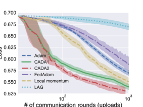
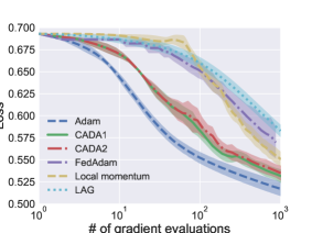
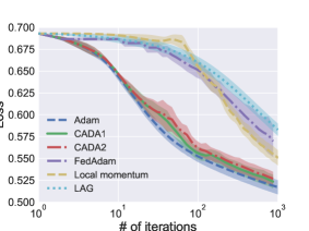
Figure 2: Logistic regression training loss on covtype dataset averaged over 10 Monte Carlo runs.

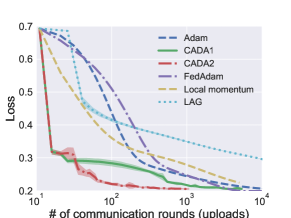
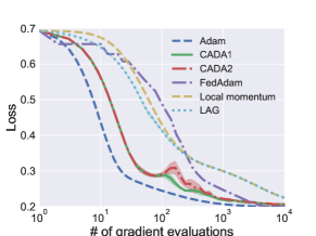
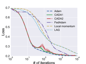
Figure 3: Logistic regression training loss on ijcnn1 dataset averaged over 10 Monte Carlo runs.

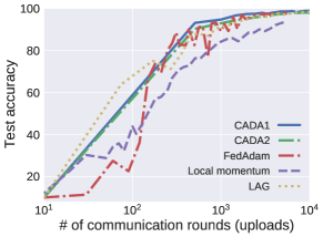
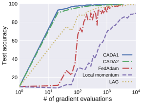
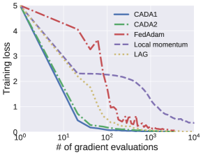
Figure 4: Training Neural network for classification on mnist dataset.

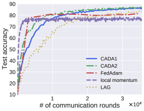
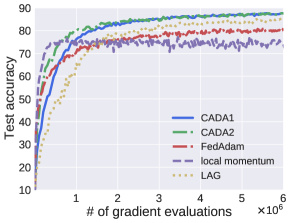
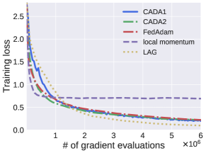
Figure 5: Training Neural network for classification on cifar10 dataset.

4 Simulations

In order to verify our analysis and show the empirical performance of CADA, we conduct simulations using logistic regression and training neural networks. Data are distributed across $M=10$ workers during all tests. We benchmark CADA with some popular methods such as Adam [Kingma and Ba(2014)], stochastic version of LAG [Chen et al.(2018)Chen, Giannakis, Sun, and Yin], local momentum [Yu et al.(2019)Yu, Jin, and Yang] and the state-of-the-art FedAdam [Reddi et al.(2020)Reddi, Charles, Zaheer, Garrett, Rush, Konečnỳ, Kumar, and McMahan]. For local momentum and FedAdam, workers perform model update independently, which are averaged over all workers every $H$ iterations. In simulations, critical parameters are optimized for each algorithm by a grid-search. Due to space limitation, please see the detailed choice of parameters, and additional experiments in the supplementary document.

Logistic regression. For CADA, the maximal delay is $D=100$ and $d_{\rm max}=10$. For local momentum and FedAdam, we manually optimize the averaging period as $H=10$ for ijcnn1 and $H=20$ for covtype. Results are averaged over 10 Monte Carlo runs.

Tests on logistic regression are reported in Figures 2-3. In our tests, two CADA variants achieve the similar iteration complexity as the original Adam and outperform all other baselines in most cases. Since our CADA requires two gradient evaluations per iteration, the gradient complexity (e.g., computational complexity) of CADA is higher than Adam, but still smaller than that of other baselines. For logistic regression task, CADA1 and CADA2 save the number of communication uploads by at least one order of magnitude.

Training neural networks. We train a neural network with two convolution-ELU-maxpooling layers followed by two fully-connected layers for 10 classes classification on mnist. We use the popular ResNet20 model on CIFAR10 dataset, which has 20 and roughly 0.27 million parameters. We searched the best values of $H$ from the grid $\{1,4,6,8,16\}$ to optimize the testing accuracy vs communication rounds for each algorithm. In CADA, the maximum delay is $D=50$ and the average interval $d_{\rm max}=10$. See tests under different $H$ in the supplementary material.

Tests on training neural networks are reported in Figures 4-5. In mnist, CADA1 and CADA2 save the number of communication uploads by roughly 60% than local momentum and slightly more than FedAdam. In cifar10, CADA1 and CADA2 achieve competitive performance relative to the state-of-the-art algorithms FedAdam and local momentum. We found that if we further enlarge $H$, FedAdam and local momentum converge fast at the beginning, but reached worse test accuracy (e.g., 5%-15%). It is also evident that the CADA1 and CADA2 rules achieve more communication reduction than the direct stochastic version of LAG, which verifies the intuition in Section 2.1.

5 Conclusions

While Adaptive SGD methods have been widely applied in the single-node setting, their performance in the distributed learning setting is less understood. In this paper, we have developed a communication-adaptive distributed Adam method that we term CADA, which endows an additional dimension of adaptivity to Adam tailored for its distributed implementation. CADA method leverages a set of adaptive communication rules to detect and then skip less informative communication rounds between the server and workers during distributed learning. All CADA variants are simple to implement, and have convergence rate comparable to the original Adam.

Supplementary materials for “CADA: Communication-Adaptive Distributed Adam”

In this supplementary document, we first present some basic inequalities that will be used frequently in this document, and then present the missing derivations of some claims, as well as the proofs of all the lemmas and theorems in the paper, which is followed by details on our experiments. The content of this supplementary document is summarized as follows.

6 Supporting Lemmas

Define the $\sigma$-algebra $\Theta^{k}=\{\theta^{l},1\leq l\leq k\}$. For convenience, we also initialize parameters as $\theta^{-D},\theta^{-D+1},\ldots,\theta^{-1}=\theta^{0}$. Some basic facts used in the proof are reviewed as follows.

Fact 1. Assume that $X_{1},X_{2},\ldots,X_{n}\in\mathbb{R}^{p}$ are independent random variables, and $EX_{1}=\cdots=EX_{n}=0$. Then

$$\mathbb{E}\Bigg{[}\Big{\|}\sum\limits_{i=1}^{n}X_{i}\Big{\|}^{2}\Bigg{]}=\sum\limits_{i=1}^{n}\mathbb{E}\left[\|X_{i}\|^{2}\right].$$ (18)

Fact 2. (Young’s inequality) For any $\theta_{1},\theta_{2}\in\mathbb{R}^{p},\varepsilon>0$,

$$\Big{\langle}\theta_{1},\theta_{2}\Big{\rangle}\leq\frac{\|\theta_{1}\|^{2}}{2\varepsilon}+\frac{\varepsilon\|\theta_{2}\|^{2}}{2}.$$ (19)

As a consequence, we have

$$\|\theta_{1}+\theta_{2}\|^{2}\leq\Big{(}1+\frac{1}{\varepsilon}\Big{)}\|\theta_{1}\|^{2}+(1+\varepsilon)\|\theta_{2}\|^{2}.$$ (20)

Fact 3. (Cauchy-Schwarz inequality) For any $\theta_{1},\theta_{2},\ldots,\theta_{n}\in\mathbb{R}^{p}$, we have

$$\Big{\|}\sum\limits_{i=1}^{n}\theta_{i}\Big{\|}^{2}\leq n\sum\limits_{i=1}^{n}\|\theta_{i}\|^{2}.$$ (21)

Lemma 6.1.

For $k-\tau_{\rm max}\leq l\leq k-D$, if $\{\theta^{k}\}$ are the iterates generated by CADA, we have

$$\mathbb{E}\left[\Big{\langle}\nabla\mathcal{L}(\theta^{k}),(\epsilon I+\hat{V}^{k-D})^{-\frac{1}{2}}\left(\nabla\ell(\theta^{l};\xi_{m}^{k})-\nabla\ell(\theta^{l};\xi_{m}^{k-\tau_{m}^{k}})\right)\Big{\rangle}\right]$$

$$\leq \frac{L\epsilon^{-\frac{1}{2}}}{12\alpha_{k}}\sum\limits_{d=1}^{D}\mathbb{E}\left[\|\theta^{k+1-d}-\theta^{k-d}\|^{2}\right]\!+\!6DL\alpha_{k}\epsilon^{-\frac{1}{2}}\sigma_{m}^{2}$$ (22)

and similarly, we have

$$\mathbb{E}\left[\Big{\langle}\nabla\mathcal{L}(\theta^{k}),(\epsilon I+\hat{V}^{k-D})^{-\frac{1}{2}}\left(\nabla\mathcal{L}_{m}(\theta^{l})-\nabla\ell(\theta^{l};\theta^{k-\tau_{m}^{k}}\right)\Big{\rangle}\right]$$

$$\leq \frac{L\epsilon^{-\frac{1}{2}}}{12\alpha_{k}}\sum\limits_{d=1}^{D}\mathbb{E}\left[\|\theta^{k+1-d}-\theta^{k-d}\|^{2}\right]+{3DL\alpha_{k}\epsilon^{-\frac{1}{2}}}\sigma_{m}^{2}.$$ (23)

Proof 6.2.

We first show the following holds.

$$\mathbb{E}\left[\Big{\langle}\nabla\mathcal{L}(\theta^{l}),(\epsilon I+\hat{V}^{k-D})^{-\frac{1}{2}}\left(\nabla\ell(\theta^{l};\xi_{m}^{k})-\nabla\ell(\theta^{l};\xi_{m}^{k-\tau_{m}^{k}})\right)\Big{\rangle}\right]$$

$$\stackrel{{\scriptstyle(a)}}{{=}} \mathbb{E}\left[\mathbb{E}\Big{[}\Big{\langle}\nabla\mathcal{L}(\theta^{l}),(\epsilon I+\hat{V}^{k-D})^{-\frac{1}{2}}\left(\nabla\ell(\theta^{l};\xi_{m}^{k})-\nabla\ell(\theta^{l};\xi_{m}^{k-\tau_{m}^{k}})\right)\Big{\rangle}\Big{|}\Theta^{l}\Big{]}\right]$$

$$\stackrel{{\scriptstyle(b)}}{{=}} \mathbb{E}\left[\Big{\langle}\nabla\mathcal{L}(\theta^{l}),(\epsilon I+\hat{V}^{k-D})^{-\frac{1}{2}}\mathbb{E}\Big{[}\nabla\ell(\theta^{l};\xi_{m}^{k})-\nabla\ell(\theta^{l};\xi_{m}^{k-\tau_{m}^{k}})\big{|}\Theta^{l}\Big{]}\Big{\rangle}\right]$$

$$= \mathbb{E}\left[\Big{\langle}\nabla\mathcal{L}(\theta^{l}),(\epsilon I+\hat{V}^{k-D})^{-\frac{1}{2}}\left(\nabla\mathcal{L}_{m}(\theta^{l})-\nabla\mathcal{L}_{m}(\theta^{l})\right)\Big{\rangle}\right]=0$$ (24)

where (a) follows from the law of total probability, and (b) holds because $\hat{V}^{k-D}$ is deterministic conditioned on $\Theta^{l}$ when $k-D\leq l$.

We first prove (6.1) by decomposing it as

$$\mathbb{E}\left[\Big{\langle}\nabla\mathcal{L}(\theta^{k}),(\epsilon I+\hat{V}^{k-D})^{-\frac{1}{2}}\left(\nabla\ell(\theta^{l};\xi_{m}^{k})-\nabla\ell(\theta^{l};\xi_{m}^{k-\tau_{m}^{k}})\right)\Big{\rangle}\right]$$

$$\stackrel{{\scriptstyle(c)}}{{=}} \mathbb{E}\left[\Big{\langle}\nabla\mathcal{L}(\theta^{k})-\nabla\mathcal{L}(\theta^{l}),(\epsilon I+\hat{V}^{k-D})^{-\frac{1}{2}}\left(\nabla\ell(\theta^{l};\xi_{m}^{k})-\nabla\ell(\theta^{l};\xi_{m}^{k-\tau_{m}^{k}})\right)\Big{\rangle}\right]$$

$$\stackrel{{\scriptstyle(d)}}{{\leq}} L\mathbb{E}\left[\Big{\|}(\epsilon I+\hat{V}^{k-D})^{-\frac{1}{4}}\Big{\|}\Big{\|}\theta^{k}-\theta^{l}\Big{\|}\Big{\|}(\epsilon I+\hat{V}^{k-D})^{-\frac{1}{4}}\left(\nabla\ell(\theta^{l};\xi_{m}^{k})-\nabla\ell(\theta^{l};\xi_{m}^{k-\tau_{m}^{k}})\right)\Big{\|}\right]$$

$$\stackrel{{\scriptstyle(e)}}{{\leq}} \frac{L\epsilon^{-\frac{1}{2}}}{12D\alpha_{k}}\underbracket{\mathbb{E}\left[\|\theta^{k}-\theta^{l}\|^{2}\right]}_{I_{1}}+\frac{6DL\alpha_{k}\epsilon^{-\frac{1}{2}}}{2}\underbracket{\mathbb{E}\left[\|\nabla\ell(\theta^{l};\xi_{m}^{k})-\nabla\ell(\theta^{l};\xi_{m}^{k-\tau_{m}^{k}})\|^{2}\right]}_{I_{2}}$$ (25)

where (c) holds due to (6.2), (d) uses Assumption 1, and (e) applies the Young’s inequality.

Applying the Cauchy-Schwarz inequality to $I_{1}$, we have

$$I_{1}= \mathbb{E}\Big{[}\Big{\|}\sum\limits_{d=1}^{k-l}(\theta^{k+1-d}-\theta^{k-d})\Big{\|}^{2}\Big{]}$$

$$\leq (k-l)\sum\limits_{d=1}^{k-l}\mathbb{E}\Big{[}\|\theta^{k+1-d}-\theta^{k-d}\|^{2}\Big{]}\leq D\sum\limits_{d=1}^{D}\mathbb{E}\Big{[}\|\theta^{k+1-d}-\theta^{k-d}\|^{2}\Big{]}.$$ (26)

Applying Assumption 2 to $I_{2}$, we have

$$I_{2}= \mathbb{E}\Big{[}\big{\|}\nabla\ell(\theta^{l};\xi_{m}^{k})-\nabla\ell(\theta^{l};\xi_{m}^{k-\tau_{m}^{k}})\big{\|}^{2}\Big{]}$$

$$= \mathbb{E}\Big{[}\big{\|}\nabla\ell(\theta^{l};\xi_{m}^{k})\big{\|}^{2}\Big{]}+\mathbb{E}\Big{[}\big{\|}\nabla\ell(\theta^{l};\xi_{m}^{k-\tau_{m}^{k}})\big{\|}^{2}\Big{]}\leq 2\sigma_{m}^{2}$$ (27)

where the last inequality uses Assumption 2. Plugging (6.2) and (6.2) into (6.2), it leads to (6.1).

Likewise, following the steps to (6.2), it can be verified that (6.1) also holds true.

Lemma 6.3.

Under Assumption 2, the parameters $\{h^{k},\hat{v}^{k}\}$ of CADA in Algorithm 1 satisfy

$$\|h^{k}\|\leq\sigma,~{}~{}~{}\forall k;~{}~{}~{}\hat{v}_{i}^{k}\leq\sigma^{2},~{}~{}~{}\forall k,i$$ (28)

where $\sigma:=\frac{1}{M}\sum_{m\in{\cal M}}\sigma_{m}$.

Proof 6.4.

Using Assumption 2, it follows that

$$\|\bm{\nabla}^{k}\|=\left\|\frac{1}{M}\sum_{m\in{\cal M}}\nabla\ell(\theta^{k-\tau_{m}^{k}};\xi_{m}^{k-\tau_{m}^{k}})\right\|\leq\frac{1}{M}\sum_{m\in{\cal M}}\left\|\nabla\ell(\theta^{k-\tau_{m}^{k}};\xi_{m}^{k-\tau_{m}^{k}})\right\|\leq\frac{1}{M}\sum_{m\in{\cal M}}\sigma_{m}=\sigma.$$ (29)

Therefore, from the update (2a), we have

$$\|h^{k+1}\|\leq\beta_{1}\|h^{k}\|+(1-\beta_{1})\|\bm{\nabla}^{k}\|\leq\beta_{1}\|h^{k}\|+(1-\beta_{1})\sigma.$$

Since $\|h^{1}\|\leq\sigma$, if follows by induction that $\|h^{k+1}\|\leq\sigma,~{}\forall k$.

Using Assumption 2, it follows that

$$(\nabla_{i}^{k})^{2} =\left(\frac{1}{M}\sum_{m\in{\cal M}}\nabla_{i}\ell(\theta^{k-\tau_{m}^{k}};\xi_{m}^{k-\tau_{m}^{k}})\right)^{2}$$

$$\leq\frac{1}{M}\sum_{m\in{\cal M}}\left(\nabla_{i}\ell(\theta^{k-\tau_{m}^{k}};\xi_{m}^{k-\tau_{m}^{k}})\right)^{2}$$

$$\leq\frac{1}{M}\sum_{m\in{\cal M}}\left\|\nabla\ell(\theta^{k-\tau_{m}^{k}};\xi_{m}^{k-\tau_{m}^{k}})\right\|^{2}=\frac{1}{M}\sum_{m\in{\cal M}}\sigma_{m}^{2}\leq\sigma^{2}.$$ (30)

Similarly, from the update (2b), we have

$$\hat{v}_{i}^{k+1}\leq\max\{\hat{v}_{i}^{k},\beta_{2}\hat{v}_{i}^{k}+(1-\beta_{2})(\nabla_{i}^{k})^{2}\}\leq\max\{\hat{v}_{i}^{k},\beta_{2}\hat{v}_{i}^{k}+(1-\beta_{2})\sigma^{2}\}.$$

Since $v_{i}^{1}=\hat{v}_{i}^{1}\leq\sigma^{2}$, if follows by induction that $\hat{v}_{i}^{k+1}\leq\sigma^{2}$.

Lemma 6.5.

Under Assumption 2, the iterates $\{\theta^{k}\}$ of CADA in Algorithm 1 satisfy

$$\left\|\theta^{k+1}-\theta^{k}\right\|^{2}\leq\alpha_{k}^{2}p(1-\beta_{2})^{-1}(1-\beta_{3})^{-1}$$ (31)

where $p$ is the dimension of $\theta$, $\beta_{1}<\sqrt{\beta_{2}}<1$, and $\beta_{3}:=\beta_{1}^{2}/\beta_{2}$.

Proof 6.6.

Choosing $\beta_{1}<1$ and defining $\beta_{3}:=\beta_{1}^{2}/\beta_{2}$, it can be verified that

$$|h_{i}^{k+1}| =\left|\beta_{1}h^{k}_{i}+(1-\beta_{1})\nabla^{k}_{i}\right|\beta_{1}|h_{i}^{k}|+|\nabla_{i}^{k}|$$

$$\leq\beta_{1}\left(\beta_{1}|h_{i}^{k-1}|+|\nabla_{i}^{k-1}|\right)+|\nabla_{i}^{k}|$$

$$\leq\sum\limits_{l=0}^{k}\beta_{1}^{k-l}|\nabla_{i}^{l}|=\sum\limits_{l=0}^{k}\sqrt{\beta_{3}}^{k-l}\sqrt{\beta_{2}}^{k-l}|\nabla_{i}^{l}|$$

$$\stackrel{{\scriptstyle(a)}}{{\leq}}\left(\sum\limits_{l=0}^{k}\beta_{3}^{k-l}\right)^{\frac{1}{2}}\left(\sum\limits_{l=0}^{k}\beta_{2}^{k-l}(\nabla_{i}^{l})^{2}\right)^{\frac{1}{2}}$$

$$\leq(1-\beta_{3})^{-\frac{1}{2}}\left(\sum\limits_{l=0}^{k}\beta_{2}^{k-l}(\nabla_{i}^{l})^{2}\right)^{\frac{1}{2}}$$ (32)

where (a) follows from the Cauchy-Schwartz inequality.

For $\hat{v}_{i}^{k}$, first we have that $\hat{v}_{i}^{1}\geq(1-\beta_{2})(\nabla_{i}^{1})^{2}$. Then since

$$\hat{v}_{i}^{k+1}\geq\beta_{2}\hat{v}_{i}^{k}+(1-\beta_{2})(\nabla_{i}^{k})^{2}$$

by induction we have

$$\hat{v}_{i}^{k+1}\geq(1-\beta_{2})\sum\limits_{l=0}^{k}\beta_{2}^{k-l}(\nabla_{i}^{l})^{2}.$$ (33)

Using (6.6) and (33), we have

$$|h_{i}^{k+1}|^{2}\leq (1-\beta_{3})^{-1}\left(\sum\limits_{l=0}^{k}\beta_{2}^{k-l}(\nabla_{i}^{l})^{2}\right)$$

$$\leq (1-\beta_{2})^{-1}(1-\beta_{3})^{-1}\hat{v}_{i}^{k+1}.$$

From the update (2c), we have

$$\|\theta^{k+1}-\theta^{k}\|^{2} =\alpha_{k}^{2}\sum_{i=1}^{p}\left(\epsilon+\hat{v}^{k+1}_{i}\right)^{-1}|h_{i}^{k+1}|^{2}$$

$$\leq\alpha_{k}^{2}p(1-\beta_{2})^{-1}(1-\beta_{3})^{-1}$$ (34)

which completes the proof.

7 Missing Derivations in Section 2.2

The analysis in this part is analogous to that in [Ghadimi and Lan(2013)]. We define an auxiliary function as

$$\psi_{m}(\theta)={\cal L}_{m}(\theta)-{\cal L}_{m}(\theta^{\star})-\Big{\langle}\nabla{\cal L}_{m}(\theta^{\star}),\theta-\theta^{\star}\Big{\rangle}$$

where $\theta^{\star}$ is a minimizer of ${\cal L}$. Assume that $\nabla\ell(\theta;\xi_{m})$ is $\bar{L}$-Lipschitz continuous for all $\xi_{m}$, we have

$$\|\nabla\ell(\theta;\xi_{m})-\nabla\ell(\theta^{\star};\xi_{m})\|^{2}\leq 2\bar{L}\left(\ell(\theta;\xi_{m})-\ell(\theta^{\star};\xi_{m})-\Big{\langle}\nabla\ell(\theta^{\star};\xi_{m}),\theta-\theta^{\star}\Big{\rangle}\right).$$

Taking expectation with respect to $\xi_{m}$, we can obtain

$$\mathbb{E}_{\xi_{m}}[\|\nabla\ell(\theta;\xi_{m})-\nabla\ell(\theta^{\star};\xi_{m})\|^{2}]\leq 2\bar{L}\left({\cal L}_{m}(\theta)-{\cal L}_{m}(\theta^{\star})-\Big{\langle}\nabla{\cal L}_{m}(\theta^{\star}),\theta-\theta^{\star}\Big{\rangle}\right)=2\bar{L}\psi_{m}(\theta).$$

Note that $\nabla{\cal L}_{m}$ is also $\bar{L}$-Lipschitz continuous and thus

$$\|\nabla{\cal L}_{m}(\theta)-\nabla{\cal L}_{m}(\theta^{\star})\|^{2}\leq 2\bar{L}({\cal L}_{m}(\theta)-{\cal L}_{m}(\theta^{\star})-\Big{\langle}\nabla{\cal L}_{m}(\theta^{\star}),\theta-\theta^{\star}\Big{\rangle})=2\bar{L}\psi_{m}(\theta).$$

7.1 Derivations of (6)

By (21), we can derive that

$$\|\theta_{1}+\theta_{2}\|\leq 2\|\theta_{1}\|^{2}+2\|\theta_{2}\|^{2}$$

which also implies $\|\theta_{1}\|^{2}\geq\frac{1}{2}\|\theta_{1}+\theta_{2}\|^{2}-\|\theta_{2}\|^{2}$.

As a consequence, we can obtain

$$\mathbb{E}\Big{[}\big{\|}\nabla\ell(\theta^{k};\xi_{m}^{k})-\nabla\ell(\theta^{k-\tau_{m}^{k}};\xi_{m}^{k-\tau_{m}^{k}})\big{\|}^{2}\Big{]}$$

$$\geq \frac{1}{2}\mathbb{E}\Big{[}\big{\|}\big{(}\nabla\ell(\theta^{k};\xi_{m}^{k})-\nabla{\cal L}_{m}(\theta^{k})\big{)}+\big{(}\nabla{\cal L}_{m}(\theta^{k-\tau_{m}^{k}})-\nabla\ell(\theta^{k-\tau_{m}^{k}};\xi_{m}^{k-\tau_{m}^{k}})\big{)}\big{\|}^{2}\Big{]}$$

$$\qquad\qquad\qquad\qquad\qquad\qquad\qquad\qquad\qquad\qquad\qquad\qquad\quad~{}~{}-\mathbb{E}\Big{[}\big{\|}\nabla{\cal L}_{m}(\theta^{k})-\nabla{\cal L}_{m}(\theta^{k-\tau_{m}^{k}})\big{\|}^{2}\Big{]}$$

$$= \frac{1}{2}\mathbb{E}\Big{[}\big{\|}\nabla\ell(\theta^{k};\xi_{m}^{k})-\nabla{\cal L}_{m}(\theta^{k})\big{\|}^{2}\Big{]}+\frac{1}{2}\mathbb{E}\Big{[}\big{[}\big{\|}\nabla\ell(\theta^{k-\tau_{m}^{k}};\xi_{m}^{k-\tau_{m}^{k}})-\nabla{\cal L}_{m}(\theta^{k-\tau_{m}^{k}})\big{\|}^{2}\big{]}\Big{]}$$

$$+\underbracket{\mathbb{E}\Big{[}\Big{\langle}\nabla\ell(\theta^{k};\xi_{m}^{k})-\nabla{\cal L}_{m}(\theta^{k}),\nabla{\cal L}_{m}(\theta^{k-\tau_{m}^{k}})-\nabla\ell(\theta^{k-\tau_{m}^{k}};\xi_{m}^{k-\tau_{m}^{k}})\Big{\rangle}\Big{]}}_{I_{3}}-\mathbb{E}\Big{[}\big{\|}\nabla{\cal L}_{m}(\theta^{k})-\nabla{\cal L}_{m}(\theta^{k-\tau_{m}^{k}})\big{\|}^{2}\Big{]}$$

where we used the fact that $I_{3}=0$ to obtain (6), that is

$$I_{3}=\mathbb{E}\Big{[}\Big{\langle}\mathbb{E}\big{[}\nabla\ell(\theta^{k};\xi_{m}^{k})\big{|}\Theta^{k}\big{]}-\nabla{\cal L}_{m}(\theta^{k}),\nabla{\cal L}_{m}(\theta^{k-\tau_{m}^{k}})-\nabla\ell(\theta^{k-\tau_{m}^{k}};\xi_{m}^{k-\tau_{m}^{k}})\Big{\rangle}\Big{]}=0.$$

7.2 Derivations of (9)

Recall that

$$\tilde{\delta}_{m}^{k}-\tilde{\delta}_{m}^{k-\tau_{m}^{k}}= \big{(}\nabla\ell(\theta^{k};\xi_{m}^{k})-\nabla\ell(\tilde{\theta};\xi_{m}^{k})+\nabla{\cal L}_{m}(\tilde{\theta})\big{)}-\big{(}\nabla\ell(\theta^{k-\tau_{m}^{k}};\xi_{m}^{k-\tau_{m}^{k}})-\nabla\ell(\tilde{\theta};\xi_{m}^{k-\tau_{m}^{k}})+\nabla{\cal L}_{m}(\tilde{\theta})\big{)}$$

$$= \underbracket{\big{(}\nabla\ell(\theta^{k};\xi_{m}^{k})-\nabla\ell(\tilde{\theta};\xi_{m}^{k})+\nabla\psi_{m}(\tilde{\theta})\big{)}}_{g_{m}^{k}}-\underbracket{\big{(}\nabla\ell(\theta^{k-\tau_{m}^{k}};\xi_{m}^{k-\tau_{m}^{k}})-\nabla\ell(\tilde{\theta};\xi_{m}^{k-\tau_{m}^{k}})+\nabla\psi_{m}(\tilde{\theta})\big{)}}_{g_{m}^{k-\tau_{m}^{k}}}.$$

And by (21), we have $\|\tilde{\delta}_{m}^{k}-\tilde{\delta}_{m}^{k-\tau_{m}^{k}}\|^{2}\leq 2\|g_{m}^{k}\|^{2}+2\|g_{m}^{k-\tau_{m}^{k}}\|^{2}$. We decompose the first term as

$$\mathbb{E}[\|g_{m}^{k}\|^{2}]\leq 2\mathbb{E}[\|\nabla\ell(\theta^{k};\xi_{m}^{k})-\nabla\ell(\theta^{\star};\xi_{m}^{k})\|^{2}]+2\mathbb{E}[\|\nabla\ell(\tilde{\theta};\xi_{m}^{k})-\nabla\ell(\theta^{\star};\xi_{m}^{k})-\nabla\psi_{m}(\tilde{\theta})\|^{2}]$$

$$= 2\mathbb{E}[\mathbb{E}[\|\nabla\ell(\theta^{k};\xi_{m}^{k})-\nabla\ell(\theta^{\star};\xi_{m}^{k})\|^{2}|\Theta^{k}]]$$

$$+2\mathbb{E}[\|\nabla\ell(\tilde{\theta};\xi_{m}^{k})-\nabla\ell(\theta^{\star};\xi_{m}^{k})-\mathbb{E}[\nabla\ell(\tilde{\theta};\xi_{m}^{k})-\nabla\ell(\theta^{\star};\xi_{m}^{k})|\Theta^{k}]\|^{2}]$$

$$\leq 4\bar{L}\mathbb{E}\psi_{m}(\theta^{k})+2\mathbb{E}[\|\nabla\ell(\tilde{\theta};\xi_{m}^{k})-\nabla\ell(\theta^{\star};\xi_{m}^{k})\|^{2}]$$

$$= 4\bar{L}\mathbb{E}\psi_{m}(\theta^{k})+2\mathbb{E}[\mathbb{E}[\|\nabla\ell(\tilde{\theta};\xi_{m}^{k})-\nabla\ell(\theta^{\star};\xi_{m}^{k})\|^{2}|\Theta^{k}]]$$

$$\leq 4\bar{L}\mathbb{E}\psi_{m}(\theta^{k})+4\bar{L}\mathbb{E}\psi_{m}(\tilde{\theta}).$$

By nonnegativity of $\psi_{m}$, we have

$$\mathbb{E}[\|g_{m}^{k}\|^{2}] \leq 4\bar{L}\sum\limits_{m\in{\cal M}}\mathbb{E}\psi_{m}(\theta^{k})+4\bar{L}\sum\limits_{m\in{\cal M}}\mathbb{E}\psi_{m}(\tilde{\theta})$$

$$=4M\bar{L}(\mathbb{E}{\cal L}(\theta^{k})-{\cal L}(\theta^{\star}))+4M\bar{L}(\mathbb{E}{\cal L}(\tilde{\theta})-{\cal L}(\theta^{\star})).$$ (35)

Similarly, we can prove

$$\mathbb{E}[\|g_{m}^{k-\tau_{m}^{k}}\|^{2}]\leq 4M\bar{L}(\mathbb{E}{\cal L}(\theta^{k-\tau_{m}^{k}})-{\cal L}(\theta^{\star}))+4M\bar{L}(\mathbb{E}{\cal L}(\tilde{\theta})-{\cal L}(\theta^{\star})).$$ (36)

Therefore, it follows that

$$\mathbb{E}[\|\tilde{\delta}_{m}^{k} -\tilde{\delta}_{m}^{k-\tau_{m}^{k}}\|^{2}]$$

$$\leq 8M\bar{L}(\mathbb{E}{\cal L}(\theta^{k})-{\cal L}(\theta^{\star}))+8M\bar{L}(\mathbb{E}{\cal L}(\theta^{k-\tau_{m}^{k}})-{\cal L}(\theta^{\star}))+16M\bar{L}(\mathbb{E}{\cal L}(\tilde{\theta})-{\cal L}(\theta^{\star})).$$

7.3 Derivations of (11)

The LHS of (10) can be written as

$$\nabla\ell(\theta^{k};\xi_{m}^{k})-\nabla\ell(\theta^{k-\tau_{m}^{k}};\xi_{m}^{k})= \big{(}\nabla\ell(\theta^{k};\xi_{m}^{k})-\nabla\ell(\theta^{k-\tau_{m}^{k}};\xi_{m}^{k})+\nabla{\cal L}_{m}(\theta^{k-\tau_{m}^{k}})\big{)}-\nabla{\cal L}_{m}(\theta^{k-\tau_{m}^{k}})$$

$$= \big{(}\nabla\ell(\theta^{k};\xi_{m}^{k})-\nabla\ell(\theta^{k-\tau_{m}^{k}};\xi_{m}^{k})+\nabla\psi_{m}(\theta^{k-\tau_{m}^{k}})\big{)}-\nabla\psi_{m}(\theta^{k-\tau_{m}^{k}}).$$

Similar to (7.2), we can obtain

$$\mathbb{E}[\|\nabla\ell(\theta^{k};\xi_{m}^{k})-\nabla\ell(\theta^{k-\tau_{m}^{k}};\xi_{m}^{k}) +\nabla\psi_{m}(\theta^{k-\tau_{m}^{k}})\|^{2}]$$

$$\leq 4M\bar{L}(\mathbb{E}{\cal L}(\theta^{k})-{\cal L}(\theta^{\star}))+4M\bar{L}(\mathbb{E}{\cal L}(\theta^{k-\tau_{m}^{k}})-{\cal L}(\theta^{\star})).$$

Combined with the fact

$$\mathbb{E}[\|\nabla\psi_{m}(\theta^{k-\tau_{m}^{k}})\|^{2}] =\mathbb{E}[\|\nabla{\cal L}_{m}(\theta^{k-\tau_{m}^{k}})-\nabla{\cal L}_{m}(\theta^{\star})\|^{2}]$$

$$\leq 2\bar{L}\mathbb{E}\psi_{m}(\theta^{k-\tau_{m}^{k}})\leq 2M\bar{L}(\mathbb{E}{\cal L}(\theta^{k-\tau_{m}^{k}})-{\cal L}(\theta^{\star}))$$

we have

$$\mathbb{E}[\|\nabla\ell(\theta^{k};\xi_{m}^{k})-\nabla\ell(\theta^{k-\tau_{m}^{k}};\xi_{m}^{k})\|^{2}]\leq 8M\bar{L}(\mathbb{E}{\cal L}(\theta^{k})-{\cal L}(\theta^{\star}))+12M\bar{L}(\mathbb{E}{\cal L}(\theta^{k-\tau_{m}^{k}})-{\cal L}(\theta^{\star})).$$

8 Proof of Lemma 3.1

Using the smoothness of $\mathcal{L}(\theta)$ in Assumption 1, we have

$$\mathcal{L}(\theta^{k+1})\leq \,\mathcal{L}(\theta^{k})+\Big{\langle}\nabla\mathcal{L}(\theta^{k}),\theta^{k+1}-\theta^{k}\Big{\rangle}+\frac{L}{2}\big{\|}\theta^{k+1}-\theta^{k}\big{\|}^{2}$$

$$= \,\mathcal{L}(\theta^{k})-\alpha_{k}\Big{\langle}\nabla\mathcal{L}(\theta^{k}),(\epsilon I+\hat{V}^{k+1})^{-\frac{1}{2}}h^{k+1}\Big{\rangle}+\frac{L}{2}\big{\|}\theta^{k+1}-\theta^{k}\big{\|}^{2}.$$ (37)

We can further decompose the inner product as

$$-\Big{\langle}\nabla\mathcal{L}(\theta^{k}),(\epsilon I+\hat{V}^{k+1})^{-\frac{1}{2}}h^{k+1}\Big{\rangle}$$

$$= -(1-\beta_{1})\Big{\langle}\nabla\mathcal{L}(\theta^{k}),(\epsilon I+\hat{V}^{k})^{-\frac{1}{2}}\bm{\nabla}^{k}\Big{\rangle}\underbracket{-\beta_{1}\Big{\langle}\nabla\mathcal{L}(\theta^{k}),(\epsilon I+\hat{V}^{k})^{-\frac{1}{2}}h^{k}\Big{\rangle}}_{I_{1}^{k}}$$

$$\underbracket{-\Big{\langle}\nabla\mathcal{L}(\theta^{k}),\left((\epsilon I+\hat{V}^{k+1})^{-\frac{1}{2}}-(\epsilon I+\hat{V}^{k})^{-\frac{1}{2}}\right)h^{k+1}\Big{\rangle}}_{I_{2}^{k}}$$ (38)

where we again decompose the first inner product as

$$-(1-\beta_{1})\Big{\langle}\nabla\mathcal{L}(\theta^{k}),(\epsilon I +\hat{V}^{k})^{-\frac{1}{2}}\bm{\nabla}^{k}\Big{\rangle}=\underbracket{-(1-\beta_{1})\Big{\langle}\nabla\mathcal{L}(\theta^{k}),(\epsilon I+\hat{V}^{k-D})^{-\frac{1}{2}}\bm{\nabla}^{k}\Big{\rangle}}_{I_{3}^{k}}$$

$$\underbracket{-(1-\beta_{1})\Big{\langle}\nabla\mathcal{L}(\theta^{k}),\left((\epsilon I+\hat{V}^{k})^{-\frac{1}{2}}-(\epsilon I+\hat{V}^{k-D})^{-\frac{1}{2}}\right)\bm{\nabla}^{k}\Big{\rangle}}_{I_{4}^{k}}.$$ (39)

Next, we bound the terms $I_{1}^{k},I_{2}^{k},I_{3}^{k},I_{4}^{k}$ separately.

Taking expectation on $I_{1}^{k}$ conditioned on $\Theta^{k}$, we have

$$\mathbb{E}[I_{1}^{k}\mid\Theta^{k}] =-\mathbb{E}\left[\beta_{1}\Big{\langle}\nabla\mathcal{L}(\theta^{k}),(\epsilon I+\hat{V}^{k})^{-\frac{1}{2}}h^{k}\Big{\rangle}\mid\Theta^{k}\right]$$

$$=-\beta_{1}\Big{\langle}\nabla\mathcal{L}(\theta^{k-1}),(\epsilon I+\hat{V}^{k})^{-\frac{1}{2}}h^{k}\Big{\rangle}-\beta_{1}\Big{\langle}\nabla\mathcal{L}(\theta^{k})-\nabla\mathcal{L}(\theta^{k-1}),(\epsilon I+\hat{V}^{k})^{-\frac{1}{2}}h^{k}\Big{\rangle}$$

$$\stackrel{{\scriptstyle(a)}}{{\leq}}-\beta_{1}\Big{\langle}\nabla\mathcal{L}(\theta^{k-1}),(\epsilon I+\hat{V}^{k})^{-\frac{1}{2}}h^{k}\Big{\rangle}+\alpha_{k-1}^{-1}\beta_{1}L\big{\|}\theta^{k}-\theta^{k-1}\big{\|}^{2}$$

$$\stackrel{{\scriptstyle(b)}}{{\leq}}\beta_{1}\left(I_{1}^{k-1}+I_{2}^{k-1}+I_{3}^{k-1}+I_{4}^{k-1}\right)+\alpha_{k-1}^{-1}\beta_{1}L\big{\|}\theta^{k}-\theta^{k-1}\big{\|}^{2}$$ (40)

where follows from the $L$-smoothness of $\mathcal{L}({\mbox{\boldmath$\theta$}})$ implied by Assumption 1; and (b) uses again the decomposition (8) and (8).

Taking expectation on $I_{2}^{k}$ over all the randomness, we have

$$\mathbb{E}[I_{2}^{k}]= \mathbb{E}\Big{[}-\Big{\langle}\nabla\mathcal{L}(\theta^{k}),\left((\epsilon I+\hat{V}^{k+1})^{-\frac{1}{2}}-(\epsilon I+\hat{V}^{k})^{-\frac{1}{2}}\right)h^{k+1}\Big{\rangle}\Big{]}$$

$$= \mathbb{E}\Big{[}\sum_{i=1}^{p}\nabla_{i}\mathcal{L}(\theta^{k})h_{i}^{k+1}\Big{(}(\epsilon+\hat{v}_{i}^{k})^{-\frac{1}{2}}-(\epsilon+\hat{v}_{i}^{k+1})^{-\frac{1}{2}}\Big{)}\Big{]}$$

$$\stackrel{{\scriptstyle(d)}}{{\leq}} \mathbb{E}\Big{[}\|\nabla\mathcal{L}(\theta^{k})\|\|h^{k+1}\|\sum_{i=1}^{p}\Big{(}(\epsilon+\hat{v}_{i}^{k})^{-\frac{1}{2}}-(\epsilon+\hat{v}_{i}^{k+1})^{-\frac{1}{2}}\Big{)}\Big{]}$$

$$\stackrel{{\scriptstyle(e)}}{{\leq}} \sigma^{2}\mathbb{E}\Big{[}\sum_{i=1}^{p}\Big{(}(\epsilon+\hat{v}_{i}^{k})^{-\frac{1}{2}}-(\epsilon+\hat{v}_{i}^{k+1})^{-\frac{1}{2}}\Big{)}\Big{]}$$ (41)

where (d) follows from the Cauchy-Schwarz inequality and (e) is due to Assumption 2.

Regarding $I_{3}^{k}$, we will bound separately in Lemma 3.2.

Taking expectation on $I_{4}^{k}$ over all the randomness, we have

$$\mathbb{E}[I_{4}^{k}]= \mathbb{E}\Big{[}-(1-\beta_{1})\Big{\langle}\nabla\mathcal{L}(\theta^{k}),\left((\epsilon I+\hat{V}^{k})^{-\frac{1}{2}}-(\epsilon I+\hat{V}^{k-D})^{-\frac{1}{2}}\right)\bm{\nabla}^{k}\Big{\rangle}\Big{]}$$

$$= -(1-\beta_{1})\mathbb{E}\Big{[}\sum_{i=1}^{p}\nabla_{i}\mathcal{L}(\theta^{k})\bm{\nabla}^{k}_{i}\Big{(}(\epsilon+\hat{v}_{i}^{k})^{-\frac{1}{2}}-(\epsilon+\hat{v}_{i}^{k-D})^{-\frac{1}{2}}\Big{)}\Big{]}$$

$$\leq (1-\beta_{1})\mathbb{E}\Big{[}\|\nabla\mathcal{L}(\theta^{k})\|\|\bm{\nabla}^{k}\|\sum_{i=1}^{p}\Big{(}(\epsilon+\hat{v}_{i}^{k-D})^{-\frac{1}{2}}-(\epsilon+\hat{v}_{i}^{k})^{-\frac{1}{2}}\Big{)}\Big{]}$$

$$\leq (1-\beta_{1})\sigma^{2}\mathbb{E}\Big{[}\sum_{i=1}^{p}\Big{(}(\epsilon+\hat{v}_{i}^{k-D})^{-\frac{1}{2}}-(\epsilon+\hat{v}_{i}^{k})^{-\frac{1}{2}}\Big{)}\Big{]}.$$ (42)

Taking expectation on (8) over all the randomness, and plugging (8), (8), and (8), we have

$$\mathbb{E}[\mathcal{L}(\theta^{k+1})]-\mathbb{E}[\mathcal{L}(\theta^{k})]\leq \,-\alpha_{k}\mathbb{E}\left[\Big{\langle}\nabla\mathcal{L}(\theta^{k}),(\epsilon I+\hat{V}^{k+1})^{-\frac{1}{2}}h^{k+1}\Big{\rangle}\right]+\frac{L}{2}\mathbb{E}\left[\big{\|}\theta^{k+1}-\theta^{k}\big{\|}^{2}\right]$$

$$= \,\alpha_{k}\mathbb{E}\left[I_{1}^{k}+I_{2}^{k}+I_{3}^{k}+I_{4}^{k}\right]+\frac{L}{2}\mathbb{E}\left[\big{\|}\theta^{k+1}-\theta^{k}\big{\|}^{2}\right]$$

$$\leq -\alpha_{k}(1-\beta_{1})\mathbb{E}\left[\Big{\langle}\nabla\mathcal{L}(\theta^{k}),(\epsilon I+\hat{V}^{k-D})^{-\frac{1}{2}}\bm{\nabla}^{k}\Big{\rangle}\right]$$

$$-\alpha_{k}\beta_{1}\mathbb{E}\left[\Big{\langle}\nabla\mathcal{L}(\theta^{k-1}),(\epsilon I+\hat{V}^{k})^{-\frac{1}{2}}h^{k}\Big{\rangle}\right]$$

$$+\alpha_{k}\sigma^{2}\mathbb{E}\Big{[}\sum_{i=1}^{p}\Big{(}(\epsilon+\hat{v}_{i}^{k})^{-\frac{1}{2}}-(\epsilon+\hat{v}_{i}^{k+1})^{-\frac{1}{2}}\Big{)}\Big{]}$$

$$+\alpha_{k}(1-\beta_{1})\sigma^{2}\mathbb{E}\Big{[}\sum_{i=1}^{p}\Big{(}(\epsilon+\hat{v}_{i}^{k-D})^{-\frac{1}{2}}-(\epsilon+\hat{v}_{i}^{k})^{-\frac{1}{2}}\Big{)}\Big{]}$$

$$+\left(\frac{L}{2}+\alpha_{k}\alpha_{k-1}^{-1}\beta_{1}L\right)\mathbb{E}\left[\|\theta^{k+1}-\theta^{k}\|^{2}\right].$$ (43)

Since $(\epsilon+\hat{v}_{i}^{k})^{-\frac{1}{2}}\leq(\epsilon+\hat{v}_{i}^{k-1})^{-\frac{1}{2}}$, we have

$$\sigma^{2}\mathbb{E}\Big{[}\sum_{i=1}^{p}\!\Big{(}\!(\epsilon+\hat{v}_{i}^{k})^{-\frac{1}{2}}\!-\!(\epsilon+\hat{v}_{i}^{k+1})^{-\frac{1}{2}}\Big{)}\!+\!(1-\beta_{1})\sum_{i=1}^{p}\!\Big{(}(\epsilon+\hat{v}_{i}^{k-D})^{-\frac{1}{2}}\!-\!(\epsilon+\hat{v}_{i}^{k})^{-\frac{1}{2}}\Big{)}\Big{]}$$

$$\leq (2-\beta_{1})\sigma^{2}\mathbb{E}\Big{[}\sum_{i=1}^{p}\Big{(}(\epsilon+\hat{v}_{i}^{k-D})^{-\frac{1}{2}}-(\epsilon+\hat{v}_{i}^{k+1})^{-\frac{1}{2}}\Big{)}\Big{]}.$$ (44)

Plugging (8) into (8) leads to the statement of Lemma 3.1.

9 Proof of Lemma 3.2

We first analyze the inner produce under CADA2 and then CADA1.

First recall that $\bar{\bm{\nabla}}^{k}=\frac{1}{M}\!\sum_{m\in{\cal M}}\nabla\ell(\theta^{k};\xi_{m}^{k})$. Using the law of total probability implies that

$$\mathbb{E}\left[\Big{\langle}\nabla\mathcal{L}(\theta^{k}),(\epsilon I+\hat{V}^{k-D})^{-\frac{1}{2}}\bar{\bm{\nabla}}^{k}\Big{\rangle}\right] =\mathbb{E}\left[\mathbb{E}\left[\Big{\langle}\nabla\mathcal{L}(\theta^{k}),(\epsilon I+\hat{V}^{k-D})^{-\frac{1}{2}}\bar{\bm{\nabla}}^{k}\Big{\rangle}\mid\Theta^{k}\right]\right]$$

$$=\mathbb{E}\left[\Big{\langle}\nabla\mathcal{L}(\theta^{k}),(\epsilon I+\hat{V}^{k-D})^{-\frac{1}{2}}\mathbb{E}\left[\bar{\bm{\nabla}}^{k}\mid\Theta^{k}\right]\Big{\rangle}\right]$$

$$=\mathbb{E}\left[\left\|\nabla\mathcal{L}(\theta^{k})\right\|^{2}_{(\epsilon I+\hat{V}^{k-D})^{-\frac{1}{2}}}\right].$$ (45)

Taking expectation on $\Big{\langle}\nabla\mathcal{L}(\theta^{k}),(\epsilon I+\hat{V}^{k-D})^{-\frac{1}{2}}\bm{\nabla}^{k}\Big{\rangle}$ over all randomness, we have

$$-\mathbb{E}\left[\Big{\langle}\nabla\mathcal{L}(\theta^{k}),(\epsilon I+\hat{V}^{k-D})^{-\frac{1}{2}}\bm{\nabla}^{k}\Big{\rangle}\right]$$

$$= -\mathbb{E}\left[\Big{\langle}\nabla\mathcal{L}(\theta^{k}),(\epsilon I+\hat{V}^{k-D})^{-\frac{1}{2}}\bar{\bm{\nabla}}^{k}\Big{\rangle}\right]$$

$$-\mathbb{E}\Big{[}\Big{\langle}\nabla\mathcal{L}(\theta^{k}),(\epsilon I+\hat{V}^{k-D})^{-\frac{1}{2}}\frac{1}{M}\sum_{m\in{\cal M}}\left(\nabla\ell(\theta^{k-\tau_{m}^{k}};\xi_{m}^{k-\tau_{m}^{k}})-\nabla\ell(\theta^{k};\xi_{m}^{k})\right)\Big{\rangle}\!\Big{]}$$

$$\stackrel{{\scriptstyle(a)}}{{=}} -\mathbb{E}\left[\left\|\nabla\mathcal{L}(\theta^{k})\right\|^{2}_{(\epsilon I+\hat{V}^{k-D})^{-\frac{1}{2}}}\right]$$

$$-\frac{1}{M}\sum_{m\in{\cal M}}\mathbb{E}\Big{[}\Big{\langle}\nabla\mathcal{L}(\theta^{k}),(\epsilon I+\hat{V}^{k-D})^{-\frac{1}{2}}\left(\nabla\ell(\theta^{k-\tau_{m}^{k}};\xi_{m}^{k-\tau_{m}^{k}})-\nabla\ell(\theta^{k};\xi_{m}^{k})\right)\Big{\rangle}\!\Big{]}$$ (46)

where (a) uses (9).

Decomposing the inner product, for the CADA2 rule (10), we have

$$-\mathbb{E}\Big{[}\Big{\langle}\nabla\mathcal{L}(\theta^{k}),(\epsilon I+\hat{V}^{k-D})^{-\frac{1}{2}}\left(\nabla\ell(\theta^{k-\tau_{m}^{k}};\xi_{m}^{k-\tau_{m}^{k}})-\nabla\ell(\theta^{k};\xi_{m}^{k})\right)\Big{\rangle}\!\Big{]}$$

$$= -\mathbb{E}\Big{[}\Big{\langle}\nabla\mathcal{L}(\theta^{k}),(\epsilon I+\hat{V}^{k-D})^{-\frac{1}{2}}\left(\nabla\ell(\theta^{k-\tau_{m}^{k}};\xi_{m}^{k-\tau_{m}^{k}})-\nabla\ell(\theta^{k-\tau_{m}^{k}};\xi_{m}^{k})\right)\!\Big{\rangle}\!\Big{]}$$

$$-\mathbb{E}\Big{[}\Big{\langle}\nabla\mathcal{L}(\theta^{k}),(\epsilon I+\hat{V}^{k-D})^{-\frac{1}{2}}\left(\nabla\ell(\theta^{k-\tau_{m}^{k}};\xi_{m}^{k})-\nabla\ell(\theta^{k};\xi_{m}^{k})\right)\Big{\rangle}\Big{]}$$

$$\stackrel{{\scriptstyle(b)}}{{\leq}} \frac{L\epsilon^{-\frac{1}{2}}}{12\alpha_{k}}\sum\limits_{d=1}^{D}\mathbb{E}\left[\|\theta^{k+1-d}-\theta^{k-d}\|^{2}\right]+{6DL\alpha_{k}\epsilon^{-\frac{1}{2}}}\sigma_{m}^{2}$$

$$\!-\mathbb{E}\Big{[}\Big{\langle}\!\nabla\mathcal{L}(\theta^{k}),(\epsilon I+\hat{V}^{k-D})^{-\frac{1}{2}}\!\left(\nabla\ell(\theta^{k-\tau_{m}^{k}};\xi_{m}^{k})-\nabla\ell(\theta^{k};\xi_{m}^{k})\right)\!\!\Big{\rangle}\Big{]}\!\!$$ (47)

where (b) follows from Lemma 6.1.

Using the Young’s inequality, we can bound the last inner product in (9) as

$$-\mathbb{E}\Big{[}\Big{\langle}\nabla\mathcal{L}(\theta^{k}),(\epsilon I+\hat{V}^{k-D})^{-\frac{1}{2}}\!\left(\nabla\ell(\theta^{k-\tau_{m}^{k}};\xi_{m}^{k})-\nabla\ell(\theta^{k};\xi_{m}^{k})\right)\!\Big{\rangle}\Big{]}$$

$$\leq \frac{1}{2}\mathbb{E}\Big{[}\Big{\|}\nabla\mathcal{L}(\theta^{k})\Big{\|}^{2}_{(\epsilon I+\hat{V}^{k-D})^{-\frac{1}{2}}}\Big{]}\!+\frac{1}{2}\mathbb{E}\Big{[}\Big{\|}(\epsilon I+\hat{V}^{k-D})^{-\frac{1}{2}}\Big{\|}\Big{\|}\!\left(\nabla\ell(\theta^{k-\tau_{m}^{k}};\xi_{m}^{k})-\nabla\ell(\theta^{k};\xi_{m}^{k})\right)\!\Big{\|}^{2}\Big{]}$$

$$\stackrel{{\scriptstyle(g)}}{{\leq}} \frac{1}{2}\mathbb{E}\Big{[}\Big{\|}\nabla\mathcal{L}(\theta^{k})\Big{\|}^{2}_{(\epsilon I+\hat{V}^{k-D})^{-\frac{1}{2}}}\Big{]}+\frac{1}{2}\mathbb{E}\Big{[}\Big{\|}(\epsilon I+\hat{V}^{k-D})^{-\frac{1}{2}}\Big{\|}\Big{\|}\nabla\ell(\theta^{k-\tau_{m}^{k}};\xi_{m}^{k})-\nabla\ell(\theta^{k};\xi_{m}^{k})\Big{\|}^{2}\Big{]}$$

$$\stackrel{{\scriptstyle(h)}}{{\leq}} \frac{1}{2}\mathbb{E}\Big{[}\Big{\|}\nabla\mathcal{L}(\theta^{k})\Big{\|}^{2}_{(\epsilon I+\hat{V}^{k-D})^{-\frac{1}{2}}}\Big{]}+\frac{c}{2d_{\rm max}}\mathbb{E}\Big{[}\Big{\|}(\epsilon I+\hat{V}^{k-D})^{-\frac{1}{2}}\Big{\|}\sum\limits_{d=1}^{d_{\rm max}}\left\|\theta^{k+1-d}\!\!-\theta^{k-d}\right\|^{2}\Big{]}$$

$$\stackrel{{\scriptstyle(i)}}{{\leq}} \frac{1}{2}\mathbb{E}\Big{[}\Big{\|}\nabla\mathcal{L}(\theta^{k})\Big{\|}^{2}_{(\epsilon I+\hat{V}^{k-D})^{-\frac{1}{2}}}\Big{]}+\frac{c\epsilon^{-\frac{1}{2}}}{2d_{\rm max}}\sum\limits_{d=1}^{D}\mathbb{E}\Big{[}\left\|\theta^{k+1-d}\!\!-\theta^{k-d}\right\|^{2}\Big{]}$$ (48)

where (g) follows from the Cauchy-Schwarz inequality, and (h) uses the adaptive communication condition (10) in CADA2, and (i) follows since $\hat{V}^{k-D}$ is entry-wise nonnegative and $\left\|\theta^{k+1-d}\!\!-\theta^{k-d}\right\|^{2}$ is nonnegative.

Similarly for CADA1’s condition (7), we have

$$-\mathbb{E}\Big{[}\Big{\langle}\nabla\mathcal{L}(\theta^{k}),(\epsilon I+\hat{V}^{k-D})^{-\frac{1}{2}}\left(\nabla\ell(\theta^{k-\tau_{m}^{k}};\xi_{m}^{k-\tau_{m}^{k}})-\nabla\ell(\theta^{k};\xi_{m}^{k})\right)\Big{\rangle}\!\Big{]}$$

$$= -\mathbb{E}\Big{[}\Big{\langle}\nabla\mathcal{L}(\theta^{k}),(\epsilon I+\hat{V}^{k-D})^{-\frac{1}{2}}\left(\nabla\ell(\tilde{\theta};\xi_{m}^{k-\tau_{m}^{k}})-\nabla\ell(\tilde{\theta};\xi_{m}^{k})\right)\!\Big{\rangle}\!\Big{]}$$

$$-\mathbb{E}\Big{[}\Big{\langle}\nabla\mathcal{L}(\theta^{k}),(\epsilon I+\hat{V}^{k-D})^{-\frac{1}{2}}\left(\tilde{\delta}^{k-\tau_{m}^{k}}_{m}-\tilde{\delta}^{k}_{m})\right)\Big{\rangle}\Big{]}$$

$$\stackrel{{\scriptstyle(j)}}{{\leq}} \frac{L\epsilon^{-\frac{1}{2}}}{12\alpha_{k}}\sum\limits_{d=1}^{D}\mathbb{E}\left[\|\theta^{k+1-d}-\theta^{k-d}\|^{2}\right]+{6DL\alpha_{k}\epsilon^{-\frac{1}{2}}}\sigma_{m}^{2}\!-\mathbb{E}\Big{[}\Big{\langle}\!\nabla\mathcal{L}(\theta^{k}),(\epsilon I+\hat{V}^{k-D})^{-\frac{1}{2}}\!\left(\tilde{\delta}_{m}^{k-\tau_{m}^{k}}-\tilde{\delta}_{m}^{k}\right)\!\!\Big{\rangle}\Big{]}$$ (49)

where (j) follows from Lemma 6.1 since $\tilde{\theta}$ is a snapshot among $\{\theta^{k},\cdots,\theta^{k-D}\}$.

And the last product in (9) is bounded by

$$-\mathbb{E}\Big{[}\Big{\langle}\nabla\mathcal{L}(\theta^{k}),(\epsilon I+\hat{V}^{k-D})^{-\frac{1}{2}}\!\left(\tilde{\delta}_{m}^{k-\tau_{m}^{k}}-\tilde{\delta}_{m}^{k}\right)\!\Big{\rangle}\Big{]}$$

$$\leq \frac{1}{2}\mathbb{E}\Big{[}\Big{\|}\nabla\mathcal{L}(\theta^{k})\Big{\|}^{2}_{(\epsilon I+\hat{V}^{k-D})^{-\frac{1}{2}}}\Big{]}+\frac{c}{2}\mathbb{E}\Big{[}\Big{\|}(\epsilon I+\hat{V}^{k-D})^{-\frac{1}{2d_{\rm max}}}\Big{\|}\sum\limits_{d=1}^{d_{\rm max}}\left\|\theta^{k+1-d}\!\!-\theta^{k-d}\right\|^{2}\Big{]}$$

$$\stackrel{{\scriptstyle(i)}}{{\leq}} \frac{1}{2}\mathbb{E}\Big{[}\Big{\|}\nabla\mathcal{L}(\theta^{k})\Big{\|}^{2}_{(\epsilon I+\hat{V}^{k-D})^{-\frac{1}{2}}}\Big{]}+\frac{c\epsilon^{-\frac{1}{2}}}{2d_{\rm max}}\sum\limits_{d=1}^{D}\mathbb{E}\Big{[}\left\|\theta^{k+1-d}\!\!-\theta^{k-d}\right\|^{2}\Big{]}.$$ (50)

Combining (9)-(9) leads to the desired statement for CADA1 and CADA2.

10 Proof of Lemma 3.3

For notational brevity, we re-write the Lyapunov function (3.1) as

$${\cal V}^{k}:=\mathcal{L}(\theta^{k})-\mathcal{L}(\theta^{\star}) -c_{k}\left\langle\nabla\mathcal{L}(\theta^{k-1}),(\epsilon I+\hat{V}^{k})^{-\frac{1}{2}}h^{k}\right\rangle$$

$$+b_{k}\sum\limits_{d=0}^{D}\sum_{i=1}^{p}(\epsilon+\hat{v}_{i}^{k-d})^{-\frac{1}{2}}+\sum\limits_{d=1}^{D}\rho_{d}\|\theta^{k+1-d}-\theta^{k-d}\|^{2}$$ (51)

where $\{c_{k}\}$ are some positive constants.

Therefore, taking expectation on the difference of ${\cal V}^{k}$ and ${\cal V}^{k+1}$ in (10), we have (with $\rho_{D+1}=0$)

$$\mathbb{E}[{\cal V}^{k+1}]-\mathbb{E}[{\cal V}^{k}]= \mathbb{E}[\mathcal{L}(\theta^{k+1})]-\mathbb{E}[\mathcal{L}(\theta^{k})]-c_{k+1}\mathbb{E}\left[\left\langle\nabla\mathcal{L}(\theta^{k}),(\epsilon I+\hat{V}^{k+1})^{-\frac{1}{2}}h^{k+1}\right\rangle\right]$$

$$+c_{k}\mathbb{E}\left[\left\langle\nabla\mathcal{L}(\theta^{k-1}),(\epsilon I+\hat{V}^{k})^{-\frac{1}{2}}h^{k}\right\rangle\right]$$

$$+b_{k+1}\sum\limits_{d=0}^{D}\sum_{i=1}^{p}(\epsilon+\hat{v}_{i}^{k+1-d})^{-\frac{1}{2}}-b_{k}\sum\limits_{d=0}^{D}\sum_{i=1}^{p}(\epsilon+\hat{v}_{i}^{k-d})^{-\frac{1}{2}}$$

$$+\rho_{1}\mathbb{E}\left[\|\theta^{k+1}-\theta^{k}\|^{2}\right]+\sum\limits_{d=1}^{D}(\rho_{d+1}-\rho_{d})\mathbb{E}\left[\|\theta^{k+1-d}-\theta^{k-d}\|^{2}\right]$$

$$\stackrel{{\scriptstyle(a)}}{{\leq}} (\alpha_{k}+c_{k+1})\mathbb{E}\left[I_{1}^{k}+I_{2}^{k}+I_{3}^{k}+I_{4}^{k}\right]-c_{k}\mathbb{E}\left[I_{1}^{k-1}+I_{2}^{k-1}+I_{3}^{k-1}+I_{4}^{k-1}\right]$$

$$+b_{k+1}\sum_{i=1}^{p}\mathbb{E}\Big{[}(\epsilon+\hat{v}_{i}^{k+1})^{-\frac{1}{2}}\Big{]}-b_{k}\sum_{i=1}^{p}\mathbb{E}\Big{[}(\epsilon+\hat{v}_{i}^{k-D})^{-\frac{1}{2}}\Big{]}$$

$$+\sum\limits_{d=1}^{D}(b_{k+1}-b_{k})\sum_{i=1}^{p}\mathbb{E}\Big{[}(\epsilon+\hat{v}_{i}^{k+1-d})^{-\frac{1}{2}}\Big{]}+\left(\frac{L}{2}+\rho_{1}\right)\mathbb{E}\left[\|\theta^{k+1}-\theta^{k}\|^{2}\right]$$

$$+\sum\limits_{d=1}^{D}(\rho_{d+1}-\rho_{d})\mathbb{E}\left[\|\theta^{k+1-d}-\theta^{k-d}\|^{2}\right]$$ (52)

where (a) uses the smoothness in Assumption 1 and the definition of $I_{1}^{k},I_{2}^{k},I_{3}^{k},I_{4}^{k}$ in (8) and (8).

Note that we can bound $(\alpha_{k}+c_{k+1})\mathbb{E}\left[I_{1}^{k}+I_{2}^{k}+I_{3}^{k}+I_{4}^{k}\right]$ the same as (8) in the proof of Lemma 3.1. In addition, Lemma 3.2 implies that

$$\mathbb{E}[I_{3}^{k}]\leq -\frac{1-\beta_{1}}{2}\mathbb{E}\left[\left\|\nabla\mathcal{L}(\theta^{k})\right\|^{2}_{(\epsilon I+\hat{V}^{k-D})^{-\frac{1}{2}}}\right]$$

$$+(1-\beta_{1})\epsilon^{-\frac{1}{2}}\left(\frac{L}{12\alpha_{k}}+\frac{c}{2d_{\rm max}}\right)\sum\limits_{d=1}^{D}\mathbb{E}\left[\|\theta^{k+1-d}-\theta^{k-d}\|^{2}\right]\!+\!(1-\beta_{1})\frac{6DL\alpha_{k}\epsilon^{-\frac{1}{2}}}{M}\!\!\sum_{m\in{\cal M}}\sigma_{m}^{2}.$$ (53)

Hence, plugging Lemma 3.1 with $\alpha_{k}$ replaced by $\alpha_{k}+c_{k+1}$ into (10), together with (10), leads to

$$\mathbb{E}[{\cal V}^{k+1}]-\mathbb{E}[{\cal V}^{k}]\leq -(\alpha_{k}+c_{k+1})\left(\frac{1-\beta_{1}}{2}\right)\mathbb{E}\left[\left\|\nabla\mathcal{L}(\theta^{k})\right\|^{2}_{(\epsilon I+\hat{V}^{k-D})^{-\frac{1}{2}}}\right]$$

$$+(\alpha_{k}+c_{k+1})(1-\beta_{1})\epsilon^{-\frac{1}{2}}\left(\frac{L}{12\alpha_{k}}+\frac{c}{2d_{\rm max}}\right)\sum\limits_{d=1}^{D}\mathbb{E}\left[\|\theta^{k+1-d}-\theta^{k-d}\|^{2}\right]\!$$

$$+(\alpha_{k}+c_{k+1})(1-\beta_{1})\frac{6DL\alpha_{k}\epsilon^{-\frac{1}{2}}}{M}\sum_{m\in{\cal M}}\sigma_{m}^{2}$$

$$+((\alpha_{k}+c_{k+1})\beta_{1}-c_{k})\mathbb{E}\left[I_{1}^{k-1}+I_{2}^{k-1}+I_{3}^{k-1}+I_{4}^{k-1}\right]$$

$$+(\alpha_{k}+c_{k+1})(2-\beta_{1})\sigma^{2}\mathbb{E}\Big{[}\sum_{i=1}^{p}\Big{(}(\epsilon+\hat{v}_{i}^{k-D})^{-\frac{1}{2}}-(\epsilon+\hat{v}_{i}^{k+1})^{-\frac{1}{2}}\Big{)}\Big{]}$$

$$+b_{k+1}\sum_{i=1}^{p}\mathbb{E}\Big{[}(\epsilon+\hat{v}_{i}^{k+1})^{-\frac{1}{2}}\Big{]}-b_{k}\sum_{i=1}^{p}\mathbb{E}\Big{[}(\epsilon+\hat{v}_{i}^{k-D})^{-\frac{1}{2}}\Big{]}$$

$$+\sum\limits_{d=1}^{D}(b_{k+1}-b_{k})\sum_{i=1}^{p}\mathbb{E}\Big{[}(\epsilon+\hat{v}_{i}^{k+1-d})^{-\frac{1}{2}}\Big{]}+\sum\limits_{d=1}^{D}(\rho_{d+1}-\rho_{d})\mathbb{E}\left[\|\theta^{k+1-d}-\theta^{k-d}\|^{2}\right]$$

$$+\left(\frac{L}{2}+\rho_{1}+(\alpha_{k}+c_{k+1})\alpha_{k-1}^{-1}\beta_{1}L\right)\mathbb{E}\left[\|\theta^{k+1}-\theta^{k}\|^{2}\right].$$ (54)

Select $\alpha_{k}\leq\alpha_{k-1}$ and $c_{k}:=\sum\limits_{j=k}^{\infty}\alpha_{j}\beta_{1}^{j-k+1}\leq(1-\beta_{1})^{-1}\alpha_{k}$ so that $(\alpha_{k}+c_{k+1})\beta_{1}=c_{k}$ and

$$(\alpha_{k}+c_{k+1})(1-\beta_{1}) \leq(\alpha_{k}+(1-\beta_{1})^{-1}\alpha_{k+1})(1-\beta_{1})$$

$$\leq\alpha_{k}(1+(1-\beta_{1})^{-1})(1-\beta_{1})=\alpha_{k}(2-\beta_{1}).$$

In addition, select $b_{k}$ to ensure that $b_{k+1}\leq b_{k}$. Then it follows from (10) that

$$\mathbb{E}[{\cal V}^{k+1}]-\mathbb{E}[{\cal V}^{k}]\leq -\frac{\alpha_{k}(1-\beta_{1})}{2}\mathbb{E}\left[\left\|\nabla\mathcal{L}(\theta^{k})\right\|^{2}_{(\epsilon I+\hat{V}^{k-D})^{-\frac{1}{2}}}\right]+(2-\beta_{1})\alpha_{k}^{2}\frac{6DL\epsilon^{-\frac{1}{2}}}{M}\sum_{m\in{\cal M}}\sigma_{m}^{2}$$

$$+(2-\beta_{1})\alpha_{k}\epsilon^{-\frac{1}{2}}\left(\frac{L}{12\alpha_{k}}+\frac{c}{2d_{\rm max}}\right)\sum\limits_{d=1}^{D}\mathbb{E}\left[\|\theta^{k+1-d}-\theta^{k-d}\|^{2}\right]$$

$$+\left(\frac{(2-\beta_{1})^{2}}{(1-\beta_{1})}\alpha_{k}\sigma^{2}-b_{k}\right)\mathbb{E}\Big{[}\sum_{i=1}^{p}\Big{(}(\epsilon+\hat{v}_{i}^{k-D})^{-\frac{1}{2}}-(\epsilon+\hat{v}_{i}^{k+1})^{-\frac{1}{2}}\Big{)}\Big{]}$$

$$+\left(\frac{L}{2}+\rho_{1}+(1-\beta_{1})^{-1}L\right)\mathbb{E}\left[\|\theta^{k+1}-\theta^{k}\|^{2}\right]$$

$$+\sum\limits_{d=1}^{D}(\rho_{d+1}-\rho_{d})\mathbb{E}\left[\|\theta^{k+1-d}-\theta^{k-d}\|^{2}\right]$$ (55)

where we have also used the fact that $-(\alpha_{k}+c_{k+1})\left(\frac{1-\beta_{1}}{2}\right)\leq-\frac{\alpha_{k}(1-\beta_{1})}{2}$ since $c_{k+1}\geq 0$.

If we choose $\alpha_{k}\leq\frac{1}{L}$ for $k=1,2\ldots,K$, then it follows from (10) that

$$\mathbb{E}[{\cal V}^{k+1}]-\mathbb{E}[{\cal V}^{k}]$$

$$\leq -\frac{\alpha_{k}(1-\beta_{1})}{2}\!\left(\epsilon+\frac{\sigma^{2}}{1-\beta_{2}}\right)^{-\frac{1}{2}}\!\!\mathbb{E}\left[\left\|\nabla\mathcal{L}(\theta^{k})\right\|^{2}\right]+(2-\beta_{1})\frac{6\alpha_{k}^{2}DL\epsilon^{-\frac{1}{2}}}{M}\!\!\sum_{m\in{\cal M}}\!\!\sigma_{m}^{2}$$

$$+\underbracket{\left(\frac{(2-\beta_{1})^{2}}{(1-\beta_{1})}\alpha_{k}\sigma^{2}-b_{k}\right)}_{A^{k}}\mathbb{E}\Big{[}\sum_{i=1}^{p}\Big{(}(\epsilon+\hat{v}_{i}^{k-D})^{-\frac{1}{2}}-(\epsilon+\hat{v}_{i}^{k+1})^{-\frac{1}{2}}\Big{)}\Big{]}$$

$$+\left(\frac{L}{2}+\rho_{1}+(1-\beta_{1})^{-1}L\right)\mathbb{E}\left[\|\theta^{k+1}-\theta^{k}\|^{2}\right]$$

$$+\sum\limits_{d=1}^{D}\underbracket{\left((2-\beta_{1})\epsilon^{-\frac{1}{2}}\left(\frac{L}{12}+\frac{c\alpha_{k}}{2d_{\rm max}}\right)+\rho_{d+1}-\rho_{d}\right)}_{B_{d}^{k}}\mathbb{E}\left[\|\theta^{k+1-d}-\theta^{k-d}\|^{2}\right].$$ (56)

To ensure $A^{k}\leq 0$ and $B_{d}^{k}\leq 0$, it is sufficient to choose $\{b_{k}\}$ and $\{\rho_{d}\}$ satisfying (with $\rho_{D+1}=0$)

$$\frac{(2-\beta_{1})^{2}}{(1-\beta_{1})}\alpha_{k}\sigma^{2}-b_{k}\leq 0,\quad k=1,\cdots,K$$ (57)

$$(2-\beta_{1})\epsilon^{-\frac{1}{2}}\left(\frac{L}{12}+\frac{c\alpha_{k}}{2d_{\rm max}}\right)+\rho_{d+1}-\rho_{d}\leq 0,\quad d=1,\cdots,D.$$ (58)

Solve this system of linear equations and get

$$b_{k}=\frac{(2-\beta_{1})^{2}}{(1-\beta_{1})L}\sigma^{2},\quad k=1,\cdots,K$$ (59)

$$\rho_{d}=(2-\beta_{1})\epsilon^{-\frac{1}{2}}\left(\frac{L}{12}+\frac{c}{2Ld_{\rm max}}\right)(D-d+1),~{}~{}~{}d=1,\cdots,D$$ (60)

plugging which into (10) leads to the conclusion of Lemma 3.3.

11 Proof of Theorem 3.4

From the definition of ${\cal V}^{k}$, we have for any $k$, that

$$\mathbb{E}[{\cal V}^{k}] \geq\mathcal{L}(\theta^{k})-\mathcal{L}(\theta^{*})-c_{k}\left\langle\nabla\mathcal{L}(\theta^{k-1}),(\epsilon I+\hat{V}^{k})^{-\frac{1}{2}}h^{k}\right\rangle+\sum\limits_{d=1}^{D}\rho_{d}\|\theta^{k+1-d}-\theta^{k-d}\|^{2}$$

$$\geq-|c_{k}|\left\|\nabla\mathcal{L}(\theta^{k-1})\right\|\left\|(\epsilon I+\hat{V}^{k})^{-\frac{1}{2}}h^{k}\right\|$$

$$\geq-(1-\beta_{1})^{-1}\alpha_{k}\sigma^{2}\epsilon^{-\frac{1}{2}}$$ (61)

where we use Assumption 2 and Lemma 6.3.

By taking summation on (10) over $k=0,\cdots,K-1$, it follows from that

$$\frac{\alpha(1-\beta_{1})}{2}\left(\epsilon+\frac{\sigma^{2}}{1-\beta_{2}}\right)^{-\frac{1}{2}}\frac{1}{K}\sum\limits_{k=1}^{K}\mathbb{E}\left[\left\|\nabla\mathcal{L}(\theta^{k})\right\|^{2}\right]$$

$$\leq \frac{\mathbb{E}[{\cal V}^{1}]-\mathbb{E}[{\cal V}^{K+1}]}{K}+(2-\beta_{1})\frac{6\alpha^{2}DL\epsilon^{-\frac{1}{2}}}{M}\sum_{m\in{\cal M}}\sigma_{m}^{2}+\frac{(2-\beta_{1})^{2}}{(1-\beta_{1})}\sigma^{2}pD\epsilon^{-\frac{1}{2}}\frac{\alpha}{K}$$

$$+\left(\frac{L}{2}+\rho_{1}+(1-\beta_{1})^{-1}L\right)\frac{1}{K}\sum\limits_{k=1}^{K}\mathbb{E}\left[\|\theta^{k+1}-\theta^{k}\|^{2}\right]$$

$$\stackrel{{\scriptstyle(a)}}{{\leq}} \frac{\mathbb{E}[{\cal V}^{1}]}{K}+(2-\beta_{1})\frac{6\alpha^{2}DL\epsilon^{-\frac{1}{2}}}{M}\sum_{m\in{\cal M}}\sigma_{m}^{2}+(1-\beta_{1})^{-1}\sigma^{2}\epsilon^{-\frac{1}{2}}\frac{\alpha}{K}+\frac{(2-\beta_{1})^{2}}{(1-\beta_{1})}\sigma^{2}pD\epsilon^{-\frac{1}{2}}\frac{\alpha}{K}$$

$$+\left(\frac{L}{2}+\rho_{1}+(1-\beta_{1})^{-1}L\right)p(1-\beta_{2})^{-1}(1-\beta_{3})^{-1}\alpha^{2}$$ (62)

where (a) follows from (11) and Lemma 6.5.

Specifically, if we choose a constant stepsize $\alpha:=\frac{\eta}{\sqrt{K}}$, where $\eta>0$ is a constant, and define

$$\tilde{C}_{1}:=(2-\beta_{1})6DL\epsilon^{-\frac{1}{2}}$$ (63)

and

$$\tilde{C}_{2}:=(1-\beta_{1})^{-1}\epsilon^{-\frac{1}{2}}+\frac{(2-\beta_{1})^{2}}{(1-\beta_{1})}D\epsilon^{-\frac{1}{2}}$$ (64)

and

$$\tilde{C}_{3}:=\left(\frac{L}{2}+\rho_{1}+(1-\beta_{1})^{-1}L\right)(1-\beta_{2})^{-1}(1-\beta_{3})^{-1}$$ (65)

and

$$\tilde{C}_{4}:=\frac{1}{2}(1-\beta_{1})\left(\epsilon+\frac{\sigma^{2}}{1-\beta_{2}}\right)^{-\frac{1}{2}}$$ (66)

we can obtain from (11) that

$$\frac{1}{K}\sum\limits_{k=0}^{K-1}\mathbb{E}\left[\|\nabla\mathcal{L}(\theta^{k})\|^{2}\right]\leq \frac{\frac{\mathcal{L}(\theta^{0})-\mathcal{L}(\theta^{*})}{K}+\frac{\tilde{C}_{1}}{M}\sum_{m\in{\cal M}}\sigma_{m}^{2}\alpha^{2}+\tilde{C}_{2}p\sigma^{2}\frac{\alpha}{K}+\tilde{C}_{3}p\alpha^{2}}{\alpha\tilde{C}_{4}}$$

$$\leq \frac{\mathcal{L}(\theta^{0})-\mathcal{L}(\theta^{*})}{K\alpha\tilde{C}_{4}}+\frac{\tilde{C}_{1}\alpha}{\tilde{C}_{4}M}\sum_{m\in{\cal M}}\sigma_{m}^{2}+\tilde{C}_{2}p\frac{\sigma^{2}}{K\tilde{C}_{4}}+\frac{\tilde{C}_{3}p\alpha}{\tilde{C}_{4}}$$

$$= \frac{(\mathcal{L}(\theta^{0})-\mathcal{L}(\theta^{*}))C_{4}}{\sqrt{K}\eta}+\frac{C_{1}\eta}{\sqrt{K}M}\sum_{m\in{\cal M}}\sigma_{m}^{2}+\frac{C_{2}p\sigma^{2}}{K}+\frac{C_{3}p\eta}{\sqrt{K}}$$

where we define $C_{1}:=\tilde{C}_{1}/\tilde{C}_{4}$, $C_{2}:=\tilde{C}_{2}/\tilde{C}_{4}$, $C_{3}:=\tilde{C}_{3}/\tilde{C}_{4}$, and $C_{4}:=1/\tilde{C}_{4}$.

12 Proof of Theorem 3.5

By the PL-condition of $\mathcal{L}(\theta)$, we have

$$-\frac{\alpha_{k}(1-\beta_{1})}{2}\!\left(\epsilon+\frac{\sigma^{2}}{1-\beta_{2}}\right)^{-\frac{1}{2}}\!\!\mathbb{E}\left[\left\|\nabla\mathcal{L}(\theta^{k})\right\|^{2}\right]$$

$$\leq -\alpha_{k}\mu(1-\beta_{1})\!\left(\epsilon+\frac{\sigma^{2}}{1-\beta_{2}}\right)^{-\frac{1}{2}}\!\!\mathbb{E}\left[\mathcal{L}(\theta^{k})-\mathcal{L}(\theta^{\star})\right]$$

$$\stackrel{{\scriptstyle(a)}}{{\leq}} \!-2\alpha_{k}\mu\tilde{C}_{4}\Big{(}\mathbb{E}[{\cal V}^{k}]\!+\!c_{k}\left\langle\nabla\mathcal{L}(\theta^{k-1}),(\epsilon I+\hat{V}^{k})^{-\frac{1}{2}}h^{k}\right\rangle\!-\!b_{k}\sum\limits_{d=0}^{D}\sum_{i=1}^{p}\!(\epsilon+\hat{v}_{i}^{k-d})^{-\frac{1}{2}}-\sum\limits_{d=1}^{D}\rho_{d}\|\theta^{k+1-d}-\theta^{k-d}\|^{2}\Big{)}$$

$$\stackrel{{\scriptstyle(b)}}{{\leq}} -2\alpha_{k}\mu\tilde{C}_{4}\mathbb{E}[{\cal V}^{k}]+2\alpha_{k}^{2}\mu\tilde{C}_{4}(1-\beta_{1})^{-1}\sigma^{2}\epsilon^{-\frac{1}{2}}+2\alpha_{k}\mu\tilde{C}_{4}b_{k}\sum\limits_{d=0}^{D}\sum_{i=1}^{p}\mathbb{E}\left[(\epsilon+\hat{v}_{i}^{k-d})^{-\frac{1}{2}}\right]$$

$$+2\alpha_{k}\mu\tilde{C}_{4}\sum\limits_{d=1}^{D}\rho_{d}\mathbb{E}[\|\theta^{k+1-d}-\theta^{k-d}\|^{2}]$$ (67)

where (a) uses the definition of $\tilde{C}_{4}$ in (66), and (b) uses Assumption 2 and Lemma 6.3.

Plugging (12) into (10), we have

$$\mathbb{E}[{\cal V}^{k+1}] -\mathbb{E}[{\cal V}^{k}]\leq-2\alpha_{k}\mu\tilde{C}_{4}\mathbb{E}[{\cal V}^{k}]+(2-\beta_{1})\frac{6\alpha_{k}^{2}DL\epsilon^{-\frac{1}{2}}}{M}\!\!\sum_{m\in{\cal M}}\!\!\sigma_{m}^{2}$$ (68)

$$+\frac{(2-\beta_{1})^{2}}{(1-\beta_{1})}\alpha_{k}\sigma^{2}\mathbb{E}\Big{[}\sum_{i=1}^{p}\Big{(}(\epsilon+\hat{v}_{i}^{k-D})^{-\frac{1}{2}}-(\epsilon+\hat{v}_{i}^{k+1})^{-\frac{1}{2}}\Big{)}\Big{]}$$

$$+b_{k+1}\sum_{i=1}^{p}\mathbb{E}\Big{[}(\epsilon+\hat{v}_{i}^{k+1})^{-\frac{1}{2}}\Big{]}-(b_{k}-2\alpha_{k}\mu\tilde{C}_{4}b_{k})\sum_{i=1}^{p}\mathbb{E}\Big{[}(\epsilon+\hat{v}_{i}^{k-D})^{-\frac{1}{2}}\Big{]}$$

$$+\sum\limits_{d=1}^{D}(b_{k+1}-b_{k}+2\alpha_{k}\mu\tilde{C}_{4}b_{k})\sum_{i=1}^{p}\mathbb{E}\Big{[}(\epsilon+\hat{v}_{i}^{k+1-d})^{-\frac{1}{2}}\Big{]}$$

$$+\left(\frac{L}{2}+\rho_{1}+(1-\beta_{1})^{-1}L\right)p(1-\beta_{2})^{-1}(1-\beta_{3})^{-1}\alpha_{k}^{2}+2\alpha_{k}^{2}\mu\tilde{C}_{4}(1-\beta_{1})^{-1}\sigma^{2}\epsilon^{-\frac{1}{2}}$$

$$+\sum\limits_{d=1}^{D}\!\left((2-\beta_{1})\epsilon^{-\frac{1}{2}}\!\left(\frac{L}{12}\!+\!\frac{c\alpha_{k}}{2d_{\rm max}}\right)+\rho_{d+1}-\rho_{d}+2\alpha_{k}\mu\tilde{C}_{4}\rho_{d}\right)\!\mathbb{E}\left[\|\theta^{k+1-d}-\theta^{k-d}\|^{2}\right].$$

If we choose $b_{k}$ to ensure that $b_{k+1}\leq(1-2\alpha_{k}\mu\tilde{C}_{4})b_{k}$, then we can obtain from (68) that

$$\mathbb{E}[{\cal V}^{k+1}]-\mathbb{E}[{\cal V}^{k}]$$ (69)

$$\leq -2\alpha_{k}\mu\tilde{C}_{4}\mathbb{E}[{\cal V}^{k}]+\frac{\tilde{C}_{1}}{M}\sum_{m\in{\cal M}}\sigma_{m}^{2}\alpha_{k}^{2}+\tilde{C}_{3}p\alpha_{k}^{2}+2\mu\tilde{C}_{4}(1-\beta_{1})^{-1}\sigma^{2}\epsilon^{-\frac{1}{2}}\alpha_{k}^{2}$$

$$+\left(\frac{(2-\beta_{1})^{2}}{(1-\beta_{1})}\alpha_{k}\sigma^{2}-(1-2\alpha_{k}\mu\tilde{C}_{4})b_{k}\right)\mathbb{E}\Big{[}\sum_{i=1}^{p}\Big{(}(\epsilon+\hat{v}_{i}^{k-D})^{-\frac{1}{2}}-(\epsilon+\hat{v}_{i}^{k+1})^{-\frac{1}{2}}\Big{)}\Big{]}$$

$$+\sum\limits_{d=1}^{D}\!\left((2-\beta_{1})\epsilon^{-\frac{1}{2}}\!\left(\frac{L}{12}\!+\!\frac{c\alpha_{k}}{2d_{\rm max}}\right)+\rho_{d+1}-\rho_{d}+2\alpha_{k}\mu\tilde{C}_{4}\rho_{d}\right)\!\mathbb{E}\left[\|\theta^{k+1-d}-\theta^{k-d}\|^{2}\right].$$

If $\alpha_{k}\leq\frac{1}{L}$, we choose parameters $\{b_{k},\rho_{d}\}$ to guarantee that

$$\frac{(2-\beta_{1})^{2}}{(1-\beta_{1})L}\sigma^{2}-\Big{(}1-\frac{2\mu\tilde{C}_{4}}{L}\Big{)}b_{k}\leq 0,~{}~{}~{}\forall k$$ (70)

$$(2-\beta_{1})\!\left(\frac{L}{12}\!+\!\frac{c}{2Ld_{\rm max}}\right)\epsilon^{-\frac{1}{2}}+\rho_{d+1}-\Big{(}1-\frac{2\mu\tilde{C}_{4}}{L}\Big{)}\rho_{d}\leq 0,~{}~{}~{}d=1,\cdots,D$$ (71)

and choose $\beta_{1},\beta_{2},\epsilon$ to ensure that $1-\frac{2\mu\tilde{C}_{4}}{L}\geq 0$.

Then we have

$$\mathbb{E}[{\cal V}^{k+1}]\leq \left(1-2\alpha_{k}\mu\tilde{C}_{4}\right)\mathbb{E}[{\cal V}^{k}]+\Bigg{(}\underbracket{\frac{\tilde{C}_{1}}{M}\sum_{m\in{\cal M}}\sigma_{m}^{2}+\tilde{C}_{3}p+2\mu\tilde{C}_{4}(1-\beta_{1})^{-1}\sigma^{2}\epsilon^{-\frac{1}{2}}}_{\tilde{C}_{5}}\Bigg{)}\alpha_{k}^{2}$$

$$\leq \prod\limits_{j=0}^{k}(1-2\alpha_{j}\mu\tilde{C}_{4})\mathbb{E}[{\cal V}^{0}]+\sum\limits_{j=0}^{k}\alpha_{j}^{2}\prod\limits_{i=j+1}^{k}(1-2\alpha_{i}\mu\tilde{C}_{4})\tilde{C}_{5}.$$ (72)

If we choose $\alpha_{k}=\frac{1}{\mu(k+K_{0})\tilde{C}_{4}}\leq\frac{1}{L}$, where $K_{0}$ is a sufficiently large constant to ensure that $\alpha_{k}$ satisfies the aforementioned conditions, then we have

$$\mathbb{E}[{\cal V}^{K}]\leq \mathbb{E}[{\cal V}^{0}]\prod\limits_{k=0}^{K-1}(1-2\alpha_{k}\mu\tilde{C}_{4})+\tilde{C}_{5}\sum\limits_{k=0}^{K-1}\alpha_{k}^{2}\prod\limits_{j=k+1}^{K-1}(1-2\alpha_{j}\mu\tilde{C}_{4})$$

$$\leq \mathbb{E}[{\cal V}^{0}]\prod\limits_{k=0}^{K-1}\frac{k+K_{0}-2}{k+K_{0}}+\frac{\tilde{C}_{5}}{\mu^{2}\tilde{C}_{4}^{2}}\sum\limits_{k=0}^{K-1}\frac{1}{(k+K_{0})^{2}}\prod\limits_{j=k+1}^{K-1}\frac{j+K_{0}-2}{j+K_{0}}$$

$$\leq \frac{(K_{0}-2)(K_{0}-1)}{(K+K_{0}-2)(K+K_{0}-1)}\mathbb{E}[{\cal V}^{0}]+\frac{\tilde{C}_{5}}{\mu^{2}\tilde{C}_{4}^{2}}\sum\limits_{k=0}^{K-1}\frac{(k+K_{0}-1)}{(k+K_{0})(K+K_{0}-2)(K+K_{0}-2)}$$

$$\leq \frac{(K_{0}-1)^{2}}{(K+K_{0}-1)^{2}}\mathbb{E}[{\cal V}^{0}]+\frac{\tilde{C}_{5}K}{\mu^{2}\tilde{C}_{4}^{2}(K+K_{0}-1)^{2}}$$

$$= \frac{(K_{0}-1)^{2}}{(K+K_{0}-1)^{2}}(\mathcal{L}(\theta^{0})-\mathcal{L}(\theta^{\star}))+\frac{\tilde{C}_{5}K}{\mu^{2}\tilde{C}_{4}^{2}(K+K_{0}-2)^{2}}$$

from which the proof is complete.

13 Additional Numerical Results

13.1 Simulation setup

In order to verify our analysis and show the empirical performance of CADA, we conduct experiments in the logistic regression and training neural network tasks, respectively.

In logistic regression, we tested the covtype and ijcnn1 in the main paper, and MNIST in the supplementary document. In training neural networks, we tested MNIST dataset in the main paper, and CIFAR10 in the supplementary document. To benchmark CADA, we compared it with some state-of-the-art algorithms, namely ADAM [Kingma and Ba(2014)], stochastic LAG, local momentum [Yu et al.(2019)Yu, Jin, and Yang, Wang et al.(2020b)Wang, Tantia, Ballas, and Rabbat] and FedAdam [Reddi et al.(2020)Reddi, Charles, Zaheer, Garrett, Rush, Konečnỳ, Kumar, and McMahan].

All experiments are run on a workstation with an Intel i9-9960x CPU with 128GB memory and four NVIDIA RTX 2080Ti GPUs each with 11GB memory using Python 3.6.

13.2 Simulation details

13.2.1 Logistic regression.

Objective function. For the logistic regression task, we use either the logistic loss for the binary case, or the cross-entropy loss for the multi-class class, both of which are augmented with an $\ell_{2}$ norm regularizer with the coefficient $\lambda=10^{-5}$.

Data pre-processing. For ijcnn1 and covtype datasets, they are imported from the popular library LIBSVM (https://www.csie.ntu.edu.tw/ cjlin/libsvm/) without further preprocessing. For MNIST, we normalize the data and subtract the mean. We uniformly partition ijcnn1 dataset with 91,701 samples and MNIST dataset with 60,000 samples into $M=10$ workers. To simulate the heterogeneous setting, we partition covtype dataset with 581,012 samples randomly into $M=20$ workers with different number of samples per worker.

For covtype, we fix the batch ratio to be 0.001 uniformly across all workers; and for ijcnn1 and MNIST, we fix the batch ratio to be 0.01 uniformly across all workers.

Choice of hyperparameters. For the logistic regression task, the hyperparameters in each algorithm are chosen by hand to roughly optimize the training loss performance of each algorithm. We list the values of parameters used in each test in Tables 1-2.

Algorithm	stepsize $\alpha$	momentum weight $\beta$	averaging interval $H/D$
FedAdam	$\alpha_{l}=100$ $\alpha_{s}=0.02$	$0.9$	$H=10$
Local momentum	$0.1$	$0.9$	$H=10$
ADAM	$0.005$	$\beta_{1}=0.9$ $\beta_{2}=0.999$	/
CADA1&2	$0.005$	$\beta_{1}=0.9$ $\beta_{2}=0.999$	$D=100$, $d_{\rm max}=10$
Stochastic LAG	$0.1$	/	$d_{\rm max}=10$

Table 1: Choice of parameters in covtype.

Algorithm	stepsize $\alpha$	momentum weight $\beta$	averaging interval $H/D$
FedAdam	$\alpha_{l}=100$ $\alpha_{s}=0.03$	$0.9$	$H=10$
Local momentum	$0.1$	$0.9$	$H=20$
ADAM	$0.01$	$\beta_{1}=0.9$ $\beta_{2}=0.999$	/
CADA	$0.01$	$\beta_{1}=0.9$ $\beta_{2}=0.999$	$D=100$, $d_{\rm max}=10$
Stochastic LAG	$0.1$	/	$d_{\rm max}=10$

Table 2: Choice of parameters in ijcnn1.

13.2.2 Training neural networks.

For training neural networks, we use the cross-entropy loss but with different network models.

Neural network models. For MNIST dataset, we use a convolutional neural network with two convolution-ELUmaxpooling layers (ELU is a smoothed ReLU) followed by two fully-connected layers. The first convolution layer is $5\times 5\times 20$ with padding, and the second layer is $5\times 5\times 50$ with padding. The output of second layer is followed by two fully connected layers with one being $800\times 500$ and the other being $500\times 10$. The output goes through a softmax function. For CIFAR10 dataset, we use the popular neural network architecture ResNet20 which has 20 and roughly 0.27 million parameters. We do not use a pre-trained model.

Data pre-processing. We uniformly partition MNIST and CIFAR10 datasets into $M=10$ workers. For MNIST, we use the raw data without preprocessing. The minibatch size per worker is 12. For CIFAR10, in addition to normalizing the data and subtracting the mean, we randomly flip and crop part of the original image every time it is used for training. This is a standard technique of data augmentation to avoid over-fitting. The minibatch size for CIFAR10 is 50 per worker.

Choice of hyperparameters. For MNIST dataset which is relatively easy, the hyperparameters in each algorithm are chosen by hand to optimize the performance of each algorithm. We list the values of parameters used in each test in Table 3.

Algorithm	stepsize $\alpha$	momentum weight $\beta$	averaging interval $H/D$
FedAdam	$\alpha_{l}=0.1$ $\alpha_{s}=0.001$	$0.9$	$H=8$
Local momentum	$0.001$	$0.9$	$H=8$
ADAM	${0.0005}$	$\beta_{1}=0.9$ $\beta_{2}=0.999$	/
CADA1&2	${0.0005}$	$\beta_{1}=0.9$ $\beta_{2}=0.999$	$D=50,d_{\rm max}=10$
Stochastic LAG	$0.1$	/	$d_{\rm max}=10$

Table 3: Choice of parameters in multi-class MNIST.

For CIFAR10 dataset, we search the best values of hyperparameters from the following search grid on a per-algorithm basis to optimize the testing accuracy versus the number of communication rounds. The chosen values of parameter are listed in Table 4.

FedAdam: $\alpha_{s}\in\left\{0.1,0.01,0.001\right\}$; $\alpha_{l}\in\left\{1,0.5,{0.1}\right\}$; $H\in\left\{1,4,6,8,16\right\}$.

Local momentum: $\alpha\in\left\{{0.1},0.01,0.001\right\}$; $H\in\left\{1,4,6,8,16\right\}$.

CADA1: $\alpha\in\left\{0.1,{0.01},0.001\right\}$; $c\in\left\{0.05,0.1,0.3,0.6,0.9,1.2,{1.5},1.8\right\}$.

CADA2: $\alpha\in\left\{0.1,{0.01},0.001\right\}$; $c\in\left\{0.05,0.1,{0.3},0.6,0.9,1.2,1.5,1.8\right\}$.

LAG: $\alpha\in\left\{{0.1},0.01,0.001\right\}$; $c\in\left\{{0.05},0.1,0.3,0.6,0.9,1.2,1.5,1.8\right\}$.

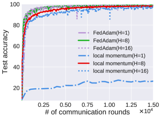
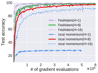
Figure 6: Performance of FedAdam and local momentum on MNIST under different $H$.

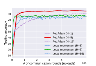
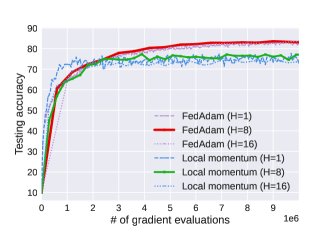
Figure 7: Performance of FedAdam and local momentum on CIFAR10 under different $H$.

Algorithm	stepsize $\alpha$	momentum weight $\beta$	averaging interval $H/D$
FedAdam	$\alpha_{l}=0.1$ $\alpha_{s}=0.1$	$0.9$	$H=8$
Local momentum	$0.1$	$0.9$	$H=8$
CADA1	$0.1$	$\beta_{1}=0.9$ $\beta_{2}=0.99$	$D=50$,  $d_{\rm max}=2$
CADA2	$0.1$	$\beta_{1}=0.9$ $\beta_{2}=0.99$	$D=50$,  $d_{\rm max}=2$
Stochastic LAG	$0.1$	/	$d_{\rm max}=2$

Table 4: Choice of parameters in CIFAR10.

Additional results. In addition to the results presented in the main paper, we report a new set of simulations on the performance of local update based algorithms under different averaging interval $H$. Since algorithms under $H=4,6$ do not perform as good as $H=8$, we only plot $H=1,8,16$ in Figures 6 and 7 to ease the comparison. Figure 6 compares the performance of FedAdam and local momentum on MNIST dataset under different averaging interval $H$. Figure 7 compares the performance of FedAdam and local momentum on CIFAR10 dataset under different $H$.

Figure 7 compares the performance of FedAdam and local momentum on CIFAR10 dataset under different averaging interval $H$. FedAdam and local momentum under a larger averaging interval $H$ have faster convergence speed at the initial stage, but they reach slightly lower testing accuracy. This reduced test accuracy is common among local SGD-type methods, which has also been studied theoretically; see e.g., [Haddadpour et al.(2019)Haddadpour, Kamani, Mahdavi, and Cadambe].

References

• [Aji and Heafield(2017)] Alham Fikri Aji and Kenneth Heafield. Sparse communication for distributed gradient descent. In Proc. Conf. Empirical Methods Natural Language Process., pages 440–445, Copenhagen, Denmark, Sep 2017.
• [Alistarh et al.(2017)Alistarh, Grubic, Li, Tomioka, and Vojnovic] Dan Alistarh, Demjan Grubic, Jerry Li, Ryota Tomioka, and Milan Vojnovic. QSGD: Communication-efficient SGD via gradient quantization and encoding. In Proc. Conf. Neural Info. Process. Syst., pages 1709–1720, Long Beach, CA, Dec 2017.
• [Alistarh et al.(2018)Alistarh, Hoefler, Johansson, Konstantinov, Khirirat, and Renggli] Dan Alistarh, Torsten Hoefler, Mikael Johansson, Nikola Konstantinov, Sarit Khirirat, and Cédric Renggli. The convergence of sparsified gradient methods. In Proc. Conf. Neural Info. Process. Syst., pages 5973–5983, Montreal, Canada, Dec 2018.
• [Bernstein et al.(2018)Bernstein, Wang, Azizzadenesheli, and Anandkumar] Jeremy Bernstein, Yu-Xiang Wang, Kamyar Azizzadenesheli, and Animashree Anandkumar. SignSGD: Compressed optimisation for non-convex problems. In Proc. Intl. Conf. Machine Learn., pages 559–568, Stockholm, Sweden, Jul 2018.
• [Bottou et al.(2018)Bottou, Curtis, and Nocedal] Léon Bottou, Frank E Curtis, and Jorge Nocedal. Optimization methods for large-scale machine learning. Siam Review, 60(2):223–311, 2018.
• [Chen et al.(2018)Chen, Giannakis, Sun, and Yin] Tianyi Chen, Georgios Giannakis, Tao Sun, and Wotao Yin. LAG: Lazily aggregated gradient for communication-efficient distributed learning. In Proc. Conf. Neural Info. Process. Syst., pages 5050–5060, Montreal, Canada, Dec 2018.
• [Chen et al.(2020)Chen, Sun, and Yin] Tianyi Chen, Yuejiao Sun, and Wotao Yin. LASG: Lazily aggregated stochastic gradients for communication-efficient distributed learning. arXiv preprint:2002.11360, 2020.
• [Chen et al.(2019)Chen, Liu, Sun, and Hong] Xiangyi Chen, Sijia Liu, Ruoyu Sun, and Mingyi Hong. On the convergence of a class of Adam-type algorithms for non-convex optimization. In Proc. Intl. Conf. Learn. Representations, New Orleans, LA, May 2019.
• [Défossez et al.(2020)Défossez, Bottou, Bach, and Usunier] Alexandre Défossez, Léon Bottou, Francis Bach, and Nicolas Usunier. On the convergence of Adam and Adagrad. arXiv preprint:2003.02395, March 2020.
• [Duchi et al.(2011)Duchi, Hazan, and Singer] John Duchi, Elad Hazan, and Yoram Singer. Adaptive subgradient methods for online learning and stochastic optimization. J. Machine Learning Res., 12(Jul):2121–2159, 2011.
• [Ghadimi and Lan(2013)] Saeed Ghadimi and Guanghui Lan. Stochastic first-and zeroth-order methods for nonconvex stochastic programming. SIAM Journal on Optimization, 23(4):2341–2368, 2013.
• [Ghadimi and Lan(2016)] Saeed Ghadimi and Guanghui Lan. Accelerated gradient methods for nonconvex nonlinear and stochastic programming. Mathematical Programming, 156(1-2):59–99, 2016.
• [Haddadpour et al.(2019)Haddadpour, Kamani, Mahdavi, and Cadambe] Farzin Haddadpour, Mohammad Mahdi Kamani, Mehrdad Mahdavi, and Viveck Cadambe. Local sgd with periodic averaging: Tighter analysis and adaptive synchronization. In Proc. Conf. Neural Info. Process. Syst., pages 11080–11092, Vancouver, Canada, December 2019.
• [Horváth et al.(2019)Horváth, Kovalev, Mishchenko, Stich, and Richtárik] Samuel Horváth, Dmitry Kovalev, Konstantin Mishchenko, Sebastian Stich, and Peter Richtárik. Stochastic distributed learning with gradient quantization and variance reduction. arXiv preprint:1904.05115, April 2019.
• [Ivkin et al.(2019)Ivkin, Rothchild, Ullah, Stoica, Arora, et al.] Nikita Ivkin, Daniel Rothchild, Enayat Ullah, Ion Stoica, Raman Arora, et al. Communication-efficient distributed SGD with sketching. In Proc. Conf. Neural Info. Process. Syst., pages 13144–13154, Vancouver, Canada, December 2019.
• [Jaggi et al.(2014)Jaggi, Smith, Takác, Terhorst, Krishnan, Hofmann, and Jordan] Martin Jaggi, Virginia Smith, Martin Takác, Jonathan Terhorst, Sanjay Krishnan, Thomas Hofmann, and Michael I Jordan. Communication-efficient distributed dual coordinate ascent. In Proc. Advances in Neural Info. Process. Syst., pages 3068–3076, Montreal, Canada, December 2014.
• [Jiang and Agrawal(2018)] Peng Jiang and Gagan Agrawal. A linear speedup analysis of distributed deep learning with sparse and quantized communication. In Proc. Conf. Neural Info. Process. Syst., pages 2525–2536, Montreal, Canada, Dec 2018.
• [Johnson and Zhang(2013)] Rie Johnson and Tong Zhang. Accelerating stochastic gradient descent using predictive variance reduction. In Proc. Conf. Neural Info. Process. Syst., pages 315–323, 2013.
• [Kairouz et al.(2019)Kairouz, McMahan, Avent, Bellet, Bennis, Bhagoji, Bonawitz, Charles, Cormode, Cummings, et al.] Peter Kairouz, H Brendan McMahan, Brendan Avent, Aurélien Bellet, Mehdi Bennis, Arjun Nitin Bhagoji, Keith Bonawitz, Zachary Charles, Graham Cormode, Rachel Cummings, et al. Advances and open problems in federated learning. arXiv preprint:1912.04977, December 2019.
• [Kamp et al.(2018)Kamp, Adilova, Sicking, Hüger, Schlicht, Wirtz, and Wrobel] Michael Kamp, Linara Adilova, Joachim Sicking, Fabian Hüger, Peter Schlicht, Tim Wirtz, and Stefan Wrobel. Efficient decentralized deep learning by dynamic model averaging. In Euro. Conf. Machine Learn. Knowledge Disc. Data.,, pages 393–409, Dublin, Ireland, 2018.
• [Karimi et al.(2016)Karimi, Nutini, and Schmidt] Hamed Karimi, Julie Nutini, and Mark Schmidt. Linear convergence of gradient and proximal-gradient methods under the polyak-łojasiewicz condition. In Proc. Euro. Conf. Machine Learn., pages 795–811, Riva del Garda, Italy, September 2016.
• [Karimireddy et al.(2019)Karimireddy, Rebjock, Stich, and Jaggi] Sai Praneeth Karimireddy, Quentin Rebjock, Sebastian Stich, and Martin Jaggi. Error feedback fixes signsgd and other gradient compression schemes. In Proc. Intl. Conf. Machine Learn., pages 3252–3261, Long Beach, CA, June 2019.
• [Karimireddy et al.(2020)Karimireddy, Kale, Mohri, Reddi, Stich, and Suresh] Sai Praneeth Karimireddy, Satyen Kale, Mehryar Mohri, Sashank J Reddi, Sebastian U Stich, and Ananda Theertha Suresh. SCAFFOLD: Stochastic controlled averaging for on-device federated learning. In Proc. Intl. Conf. Machine Learn., July 2020.
• [Kingma and Ba(2014)] Diederik P Kingma and Jimmy Ba. Adam: A method for stochastic optimization. arXiv preprint:1412.6980, December 2014.
• [Li et al.(2018)Li, Sahu, Zaheer, Sanjabi, Talwalkar, and Smith] Tian Li, Anit Kumar Sahu, Manzil Zaheer, Maziar Sanjabi, Ameet Talwalkar, and Virginia Smith. Federated optimization in heterogeneous networks. arXiv preprint arXiv:1812.06127, 2018.
• [Li and Orabona(2019)] Xiaoyu Li and Francesco Orabona. On the convergence of stochastic gradient descent with adaptive stepsizes. In Proc. Intl. Conf. on Artif. Intell. and Stat., pages 983–992, Okinawa, Japan, April 2019.
• [Lian et al.(2016)Lian, Zhang, Hsieh, Huang, and Liu] Xiangru Lian, Huan Zhang, Cho-Jui Hsieh, Yijun Huang, and Ji Liu. A comprehensive linear speedup analysis for asynchronous stochastic parallel optimization from zeroth-order to first-order. In Proc. Conf. Neural Info. Process. Syst., pages 3054–3062, Barcelona, Spain, December 2016.
• [Lin et al.(2020)Lin, Stich, Patel, and Jaggi] Tao Lin, Sebastian U Stich, Kumar Kshitij Patel, and Martin Jaggi. Don’t use large mini-batches, use local SGD. In Proc. Intl. Conf. Learn. Representations, Addis Ababa, Ethiopia, April 2020.
• [Lin et al.(2018)Lin, Han, Mao, Wang, and Dally] Yujun Lin, Song Han, Huizi Mao, Yu Wang, and William J Dally. Deep gradient compression: Reducing the communication bandwidth for distributed training. In Proc. Intl. Conf. Learn. Representations, Vancouver, Canada, Apr 2018.
• [Ma et al.(2017)Ma, Konečnỳ, Jaggi, Smith, Jordan, Richtárik, and Takáč] Chenxin Ma, Jakub Konečnỳ, Martin Jaggi, Virginia Smith, Michael I Jordan, Peter Richtárik, and Martin Takáč. Distributed optimization with arbitrary local solvers. Optimization Methods and Software, 32(4):813–848, July 2017.
• [McMahan et al.(2017a)McMahan, Moore, Ramage, Hampson, and y Arcas] Brendan McMahan, Eider Moore, Daniel Ramage, Seth Hampson, and Blaise Aguera y Arcas. Communication-efficient learning of deep networks from decentralized data. In Proc. Intl. Conf. Artificial Intell. and Stat., pages 1273–1282, Fort Lauderdale, FL, April 2017a.
• [McMahan et al.(2017b)McMahan, Moore, Ramage, Hampson, and y Arcas] Brendan McMahan, Eider Moore, Daniel Ramage, Seth Hampson, and Blaise Aguera y Arcas. Communication-efficient learning of deep networks from decentralized data. In Proc. Intl. Conf. on Artif. Intell. and Stat., pages 1273–1282, Fort Lauderdale, Florida, Apr 2017b.
• [Nesterov(1983)] Yurii E Nesterov. A method for solving the convex programming problem with convergence rate $o(1/k^{2})$. In Doklady AN USSR, volume 269, pages 543–547, 1983.
• [Park et al.(2019)Park, Samarakoon, Bennis, and Debbah] Jihong Park, Sumudu Samarakoon, Mehdi Bennis, and Mérouane Debbah. Wireless network intelligence at the edge. Proc. of the IEEE, 107(11):2204–2239, November 2019.
• [Polyak(1964)] Boris T Polyak. Some methods of speeding up the convergence of iteration methods. Computational Mathematics and Mathematical Physics, 4(5):1–17, 1964.
• [Reddi et al.(2018)Reddi, Kale, and Kumar] Sashank Reddi, Satyen Kale, and Sanjiv Kumar. On the convergence of adam and beyond. In Proc. Intl. Conf. Learn. Representations, Vancouver, Canada, April 2018.
• [Reddi et al.(2020)Reddi, Charles, Zaheer, Garrett, Rush, Konečnỳ, Kumar, and McMahan] Sashank Reddi, Zachary Charles, Manzil Zaheer, Zachary Garrett, Keith Rush, Jakub Konečnỳ, Sanjiv Kumar, and H Brendan McMahan. Adaptive federated optimization. arXiv preprint:2003.00295, March 2020.
• [Reisizadeh et al.(2019)Reisizadeh, Taheri, Mokhtari, Hassani, and Pedarsani] Amirhossein Reisizadeh, Hossein Taheri, Aryan Mokhtari, Hamed Hassani, and Ramtin Pedarsani. Robust and communication-efficient collaborative learning. In Proc. Conf. Neural Info. Process. Syst., pages 8386–8397, Vancouver, Canada, December 2019.
• [Robbins and Monro(1951)] Herbert Robbins and Sutton Monro. A stochastic approximation method. Annals of Mathematical Statistics, 22(3):400–407, September 1951.
• [Seide et al.(2014)Seide, Fu, Droppo, Li, and Yu] Frank Seide, Hao Fu, Jasha Droppo, Gang Li, and Dong Yu. 1-bit stochastic gradient descent and its application to data-parallel distributed training of speech DNNs. In Proc. Conf. Intl. Speech Comm. Assoc., Singapore, Sept 2014.
• [Shamir et al.(2014)Shamir, Srebro, and Zhang] Ohad Shamir, Nati Srebro, and Tong Zhang. Communication-efficient distributed optimization using an approximate newton-type method. In Proc. Intl. Conf. Machine Learn., pages 1000–1008, Beijing, China, Jun 2014.
• [Stich et al.(2018)Stich, Cordonnier, and Jaggi] Sebastian U. Stich, Jean-Baptiste Cordonnier, and Martin Jaggi. Sparsified SGD with memory. In Proc. Conf. Neural Info. Process. Syst., pages 4447–4458, Montreal, Canada, Dec 2018.
• [Stich(2019)] Sebastian Urban Stich. Local SGD converges fast and communicates little. In Proc. Intl. Conf. Learn. Representations, New Orleans, LA, May 2019.
• [Strom(2015)] Nikko Strom. Scalable distributed DNN training using commodity GPU cloud computing. In Proc. Conf. Intl. Speech Comm. Assoc., Dresden, Germany, September 2015.
• [Sun et al.(2019)Sun, Chen, Giannakis, and Yang] Jun Sun, Tianyi Chen, Georgios Giannakis, and Zaiyue Yang. Communication-efficient distributed learning via lazily aggregated quantized gradients. In Proc. Conf. Neural Info. Process. Syst., page to appear, Vancouver, Canada, Dec 2019.
• [Tang et al.(2018)Tang, Gan, Zhang, Zhang, and Liu] Hanlin Tang, Shaoduo Gan, Ce Zhang, Tong Zhang, and Ji Liu. Communication compression for decentralized training. In Proc. Conf. Neural Info. Process. Syst., pages 7652–7662, Montreal, Canada, December 2018.
• [Tang et al.(2020)Tang, Gan, Rajbhandari, Lian, Zhang, Liu, and He] Hanlin Tang, Shaoduo Gan, Samyam Rajbhandari, Xiangru Lian, Ce Zhang, Ji Liu, and Yuxiong He. Apmsqueeze: A communication efficient adam-preconditioned momentum sgd algorithm. arXiv preprint:2008.11343, August 2020.
• [Vogels et al.(2019)Vogels, Karimireddy, and Jaggi] Thijs Vogels, Sai Praneeth Karimireddy, and Martin Jaggi. PowerSGD: Practical low-rank gradient compression for distributed optimization. In Proc. Conf. Neural Info. Process. Syst., pages 14236–14245, Vancouver, Canada, December 2019.
• [Wang et al.(2020a)Wang, Lu, Tu, and Zhang] Guanghui Wang, Shiyin Lu, Weiwei Tu, and Lijun Zhang. SAdam: A variant of adam for strongly convex functions. In Proc. Intl. Conf. Learn. Representations, 2020a.
• [Wang and Joshi(2019)] Jianyu Wang and Gauri Joshi. Cooperative SGD: A unified framework for the design and analysis of communication-efficient SGD algorithms. In ICML Workshop on Coding Theory for Large-Scale ML, Long Beach, CA, June 2019.
• [Wang et al.(2020b)Wang, Tantia, Ballas, and Rabbat] Jianyu Wang, Vinayak Tantia, Nicolas Ballas, and Michael Rabbat. SlowMo: Improving communication-efficient distributed SGD with slow momentum. In Proc. Intl. Conf. Learn. Representations, 2020b.
• [Wangni et al.(2018)Wangni, Wang, Liu, and Zhang] Jianqiao Wangni, Jialei Wang, Ji Liu, and Tong Zhang. Gradient sparsification for communication-efficient distributed optimization. In Proc. Conf. Neural Info. Process. Syst., pages 1299–1309, Montreal, Canada, Dec 2018.
• [Ward et al.(2019)Ward, Wu, and Bottou] Rachel Ward, Xiaoxia Wu, and Leon Bottou. Adagrad stepsizes: Sharp convergence over nonconvex landscapes. In Proc. Intl. Conf. Machine Learn., pages 6677–6686, Long Beach, CA, June 2019.
• [Wen et al.(2017)Wen, Xu, Yan, Wu, Wang, Chen, and Li] Wei Wen, Cong Xu, Feng Yan, Chunpeng Wu, Yandan Wang, Yiran Chen, and Hai Li. Terngrad: Ternary gradients to reduce communication in distributed deep learning. In Proc. Conf. Neural Info. Process. Syst., pages 1509–1519, Long Beach, CA, Dec 2017.
• [Wu et al.(2018)Wu, Huang, Huang, and Zhang] Jiaxiang Wu, Weidong Huang, Junzhou Huang, and Tong Zhang. Error compensated quantized sgd and its applications to large-scale distributed optimization. In Proc. Intl. Conf. Machine Learn., pages 5325–5333, Stockholm, Sweden, Jul 2018.
• [Xu et al.(2020)Xu, Sutcher-Shepard, Xu, and Chen] Yangyang Xu, Colin Sutcher-Shepard, Yibo Xu, and Jie Chen. Asynchronous parallel adaptive stochastic gradient methods. arXiv preprint:2002.09095, February 2020.
• [Yu et al.(2019)Yu, Jin, and Yang] Hao Yu, Rong Jin, and Sen Yang. On the linear speedup analysis of communication efficient momentum SGD for distributed non-convex optimization. In Proc. Intl. Conf. Machine Learn., pages 7184–7193, Long Beach, CA, June 2019.
• [Zeiler(2012)] Matthew D Zeiler. Adadelta: an adaptive learning rate method. arXiv preprint:1212.5701, December 2012.
• [Zhang et al.(2017)Zhang, Li, Kara, Alistarh, Liu, and Zhang] Hantian Zhang, Jerry Li, Kaan Kara, Dan Alistarh, Ji Liu, and Ce Zhang. Zipml: Training linear models with end-to-end low precision, and a little bit of deep learning. In Proc. Intl. Conf. Machine Learn., pages 4035–4043, Sydney, Australia, Aug 2017.
• [Zhang et al.(2015)Zhang, Choromanska, and LeCun] Sixin Zhang, Anna E Choromanska, and Yann LeCun. Deep learning with elastic averaging SGD. In Proc. Conf. Neural Info. Process. Syst., pages 685–693, Montreal, Canada, Dec 2015.
• [Zhang and Lin(2015)] Yuchen Zhang and Xiao Lin. DiSCO: Distributed optimization for self-concordant empirical loss. In Proc. Intl. Conf. Machine Learn., pages 362–370, Lille, France, June 2015.