Linear quadratic mean field social optimization: Asymptotic solvability and decentralized control

Abstract.

This paper studies asymptotic solvability of a linear quadratic (LQ) mean field social optimization problem with controlled diffusions and indefinite state and control weights. Starting with an $N$-agent model, we employ a rescaling approach to derive a low-dimensional Riccati ordinary differential equation (ODE) system, which characterizes a necessary and sufficient condition for asymptotic solvability. The decentralized control obtained from the mean field limit ensures a bounded optimality loss in minimizing the social cost having magnitude $O(N)$, which implies an optimality loss of $O(1/N)$ per agent. We further quantify the efficiency gain of the social optimum with respect to the solution of the mean field game.

1. Introduction

In social optimization problems, multiple interacting agents have individual performance objectives but cooperatively optimize for the goal of the whole group. For instance, such scenarios arise in communication networks seeking network utility maximization, where the total utility of the users is maximized [21, 31, 40]; the extension to the case of multi-period optimization can be found in [31, 60]. Similarly, in the economic literature social welfare functions have long been studied [45, 47] as a key concept of welfare economics. A typical form that they take is the sum of the individual utilities and is accordingly called a utilitarian social welfare function.

In this paper, we are concerned with mean field social optimization involving $N$ agents which have mean field coupling through their individual dynamics and costs and minimize a social cost. Consider a system of $N$ agents, denoted by $\mathcal{A}_{i}$, $1\leq i\leq N$. The state process $X_{i}(t)$ of $\mathcal{A}_{i}$ satisfies the following stochastic differential equation (SDE)

(1.1) $$dX_{i}(t) =(AX_{i}(t)+Bu_{i}(t)+GX^{(N)}(t))dt+(B_{1}u_{i}(t)+D)dW_{i}(t)$$

$$\quad+(B_{0}u^{(N)}(t)+D_{0})dW_{0}(t),$$

where we have the state $X_{i}(t)\in\mathbb{R}^{n}$, the control $u_{i}(t)\in\mathbb{R}^{n_{1}}$, the mean field state $X^{(N)}\coloneqq(1/N)\sum_{i=1}^{N}X_{i}$, and the control mean field $u^{(N)}\coloneqq(1/N)\sum_{i=1}^{N}u_{i}$. The initial states $\{X_{i}(0):1\leq i\leq N\}$ are independent with $\mathbb{E}X_{i}(0)=x_{i}(0)$ and $\mathbb{E}|X_{i}(0)|^{2}<\infty$. The individual noise processes $\{W_{i}:1\leq i\leq N\}$ are $1$-dimensional independent standard Brownian motions, which are also independent of $\{X_{i}(0):1\leq i\leq N\}$. The common noise $W_{0}$ is a $1$-dimensional standard Brownian motion independent of $\{W_{i}:1\leq i\leq N\}$ and $\{X_{i}(0):1\leq i\leq N\}$.

The individual cost of agent ${\mathcal{A}}_{i}$, $1\leq i\leq N$, is given by

$$J_{i}(u_{1},\cdots,u_{N}) =\mathbb{E}\bigg{[}\int_{0}^{T}\Big{(}[X_{i}(t)-\Gamma X^{(N)}(t)]_{Q}^{2}+[u_{i}(t)]_{R}^{2}\Big{)}dt$$

$$\qquad+[X_{i}(T)-\Gamma_{f}X^{(N)}(T)]_{Q_{f}}^{2}\bigg{]},$$

where we denote the quadratic form $[y]_{M}^{2}=y^{T}My$ for a symmetric matrix $M$. The social cost is defined as

(1.2) $$J_{\rm soc}^{(N)}(u_{1},\cdots,u_{N}) \coloneqq\sum_{i=1}^{N}J_{i}(u_{1},\cdots,u_{N}).$$

The constant matrices $A$, $B$, $B_{0}$ $B_{1}$, $D$, $D_{0}$, $G$, $\Gamma$, $Q$, $R$, $\Gamma_{f}$ and $Q_{f}$ above have compatible dimensions, and $Q$, $R$ and $Q_{f}$ are symmetric matrices. The weight matrices $Q$, $R$ and $Q_{f}$ may be indefinite. LQ stochastic optimal control with indefinite control weights was first studied in [18], which shows that the optimal control problem may still be well posed when the control enters the diffusion term. The more general case with indefinite state and control weight matrices are treated in [54, 65]. It is shown in [54] that the solvability of the stochastic optimal control problem is equivalent to the solvability of a generalized differential Riccati-type equation. For discrete-time LQ control problems with indefinite weight matrices, see [25, 53].

The above social optimization model differs from mean field games in that the agents in the latter are non-cooperative. For general theory and applications of mean field games, the reader is referred to [7, 11, 12, 17, 15, 28, 29, 30, 35, 42]. LQ mean field games are a particularly attractive class of problems due to their explicit solutions [5, 9, 32, 33, 46, 55].

There has been a growing literature related to mean field social optimization. An LQ mean field social optimization problem has been considered in [34] with additive noise and positive definite control weight and positive semi-definite state weight. That work constructs the limiting decision problems for the individual agents by use of the person-by-person (PbP) optimality principle where a selected agent takes non-anticipative control perturbations. This method is applied to a nonlinear model in [58]. The work [20] studies social optimization with indefinite state weight. Social optima are analyzed in [61] for a mean field jump LQ model governed by a common Markovian chain. An LQ social optimum model is studied in [56] for a large number of weakly coupled agents choosing cooperatively between multiple destinations. A nonlinear social optimization problem for an infinite horizon economy is analyzed in [49], where necessary conditions of the social optimum are derived by using Gâteaux derivatives and Lagrangian multipliers treating market clearing equality constraints. A discrete-time LQ social optimization problem involving a finite number of subsystems with mean-field state coupling is analyzed in [3] to obtain optimal control laws for both full observation and partial observation cases; this problem is called team-optimization to emphasize decentralized information structures. Further analysis of the mean field limit is developed in [4]. Static mean field teams with general costs are studied in [57] under certain symmetry assumptions. It is shown that the solution obtained in the limit problem has asymptotic optimality for the model with a finite number of agents. Mean field optimal control and flocking behavior of many interacting agents can be found in [1, 27].

For a given $N$, the social optimum with the additive social cost may be viewed as a particular way of achieving a Pareto efficient solution in the sense that no individual can further improve for itself without causing at least another agent to get worse. But Pareto optimality is a much weaker optimality notion and usually contains a set of qualified solutions. The reader may consult [24] for characterization of Pareto efficient solutions in cooperative differential games. Both mean field games and mean field social optima are analyzed and compared in [14, 43]. The bounds for their efficiency difference are provided in [14] while [43] shows that the mean field equilibrium may be interpreted as the solution of a modified social optimization problem. Performance comparisons of the two solution approaches are presented in [63] for a static mean field model arising in dense wireless networks.

1.1. Related literature on mean field type optimal control

It is worthwhile to mention the related area of mean field type optimal control problems which involve the state process together with its mean [2] or its distribution (see e.g. [8, 41]). Moreover, the model involves only one decision maker, which immediately affects the distribution of the underlying state process. The optimal control is characterized by a stochastic maximum principle under a convex control set in [2], and this approach is extended to deal with more general dynamics and a possibly non-convex control set [10], which derives the maximum principle containing a second order adjoint equation. For LQ mean field type optimal control, [64] derives the solution via a system of forward-backward stochastic differential equations (FBSDEs) and further decouples the FBSDEs by Riccati equations to obtain the optimal control in an explicit form. For discrete-time mean field type control, the reader is referred to [23, 48].

Instead of just including mean terms in the model, the more general framework considers optimal control of McKean–Vlasov dynamics, where both the system state and its law appear in the dynamics and costs. The optimal control law has the interpretation of a cooperative equilibrium in a large population model of $N$ agents coupled by the empirical distribution of their states [16], but the search for this cooperative equilibrium is based on the restriction that all agents use the same local feedback control law $\varphi(t,X_{i})$ to test optimality. The connection between large population social optimal control and optimal control of McKean–Vlasov dynamics is further addressed in [41] and [22]. It is shown in [41] that the social optimal control problems of a large number of interacting state processes may be connected with optimal control problems of McKean–Vlasov type. Specifically, each relaxed optimal control of the McKean–Vlasov model may be obtained as the limit of relaxed $\epsilon_{N}$-optimal controls for the $N$-agent social optimal control problems, where $\epsilon_{N}\to 0$ as $N\to\infty$. Similar limit theorems are obtained in [22] for more general system dynamics together with common noise, where the state equation uses a conditional law of the state-control pair given the common noise. The dynamic programming approach is applied to mean field type optimal control in [8] to derive the so-called master equation. For McKean–Vlasov optimal control problems with common noise, the dynamic programming principle is established in [6, 52] by taking the distribution of the state as an abstract state subject to stochastic McKean–Vlasov dynamics. An application to LQ optimal control problems is presented in [51] dealing with positive (semi-)definite weight matrices.

While there is a close connection between large population social optimal control and McKean–Vlasov optimal control (or mean field type control in general) as analyzed in [41, 22], the two classes of models have crucial differences. Firstly, the actual mechanisms affecting the mean field are different in that a single agent in the social optimization model has little impact on the mean field. Secondly, the McKean–Vlasov optimal control model typically assumes homogeneous agents while social optimization allows heterogeneity; for instance, the LQ model in [34] allows the agents to have individual dynamic parameters varying from a continuum. Finally, the two classes of problems interpret time consistency differently, and the social optimum may easily attain time consistency due to the particular mechanism generating the mean field (this point will be illustrated by examples in Section 5.4).

1.2. Our approach

Our study of the model (1.1)–(1.2) deals with control-dependent noises and indefinite control and state weight matrices. More importantly, here we take a new perspective by adopting a notion called asymptotic solvability. Roughly speaking, asymptotic solvability, which is formally defined in Section 3, is the solvability of the social optimization problem (1.1)–(1.2) as $N\to\infty$. Some early analysis has been presented in the conference paper [36]. The asymptotic solvability approach was initially developed in LQ mean field games [38, 39]; that approach attempts to answer such a question for the games: Does there exist an intrinsic low-dimensional object that governs the large system’s solution generating a good asymptotic behavior when the population size tends to infinity. The approach shares similarity with the convergence problem in the direct approach of mean field games [13]. In [38, 39], a necessary and sufficient condition for asymptotic solvability of $N$-player LQ mean field games is obtained through analyzing a low-dimensional ODE system derived by applying a rescaling method to the sequence of high-dimensional centralized solutions. Asymptotic solvability of LQ mean field games with a major player is studied in [44].

For the $N$-agent LQ optimal control problem (1.1)–(1.2) with indefinite weights, one in principle may use a Riccati equation to determine feedback optimal control [59]. Due to the indefinite weights, the equation does not always have a solution, and determining the existence of a solution becomes a highly nontrivial task, especially when $N$ is large. This poses a conceptual obstacle before we can even think of deriving a mean field limit from a centralized solution and consider decentralized individual controls with little optimality loss. In this case, our formulation of the asymptotic solvability problem is particularly relevant for addressing this existence issue by coming up with a simple criterion. Then our further analysis will show that some simpler limiting objects (as two ODEs in a lower-dimensional space) encodes all essential information for a well behaved system when $N\to\infty$. Specifically, our starting point here is to apply dynamic programming to derive the large-scale Riccati equation. This approach has several advantages for the present model over the person-by-person optimality argument in [34]. First, the Riccati equation-based approach, as long as its solvability holds, ensures optimality from the beginning. In contrast, the PbP optimality-based approach is much harder to apply due to the common noise. Second, the large Riccati equation is particularly suitable for applying the rescaling technique as in [39]. The LQ social optimization model in [19, 34] involves positive semi-definite state weight and positive definite control weight, and the players have only independent noises.

Next, we determine the closed-loop dynamics under the centralized optimal control $U^{o}$ and use the mean field limit to derive a set of decentralized individual controls $U^{d}$ for which each agent uses only its own state and the mean field limit state. While the social optimum $J_{\rm soc}^{(N)}(U^{o})$ has magnitude $O(N)$, the decentralized control is shown to achieve bounded optimality loss with respect to the social optimum as $N\to\infty$, i.e., $0\leq J_{\rm soc}^{(N)}(U^{d})-J_{\rm soc}^{(N)}(U^{o})=O(1)$, which is tighter than the upper bound $O(\sqrt{N})$ for optimality loss obtained by the method in [34]. In [4] it is shown for a mean field team the mean field limit based policy can have an overall optimality loss of $O(1)$, but they consider a relatively simple linear model with uncontrolled noise and do not face high nonlinearity of the Riccati equation. Their model has positive definite weights, and asymptotic solvability automatically holds.

We also note that the limit theorems in [41, 22] relate mean field social optimization to control of McKean–Vlasov dynamics. Their nonlinear models have much generality but the compactness-based analysis needs restrictive conditions on the control caused growth of the cost integrand. These conditions cannot cover our indefinite quadratic cost.

1.3. Contributions and organization

We extend the asymptotic solvability notion, initially introduced for mean field games, to social optimization. A key feature of our system is that the state and control weight matrices may be indefinite. Due to the highly nonlinear Riccati ODEs resulting from controlled diffusion terms, the development of the rescaling technique is more challenging than in [38, 39, 44]. We further obtain a tight upper bound of the optimality loss of the obtained decentralized controls, and quantify the efficiency gain with respect to mean field game solutions.

The paper is organized as follows. In Section 2, we introduce the LQ mean field social optimization model and derive the large-scale Riccati equation for the optimal control. Section 3 introduces the asymptotic solvability notion and presents a necessary and sufficient condition for asymptotic solvability via a low-dimensional Riccati ODE system. Section 4 gives the closed-loop state dynamics under the optimal control and its mean field limit. Section 5 analyzes the associated decentralized control by proving a bounded optimality gap result, and compares the performance with the mean field game solution. This section also compares mean field social optimization with mean field type optimal control. Section 6 gives some numerical examples. Section 7 concludes the paper.

1.4. Notation

We use $I$ to denote an identity matrix of compatible dimensions, and sometimes write $I_{k}$ to indicate the $k\times k$ identity matrix. For a vector or matrix $F$, $|F|$ denotes the Euclidean norm of $F$. For any $l\times m$ matrix $Z=(z_{ij})_{1\leq i\leq l,1\leq j\leq m}$, we denote the $l_{1}$-norm $\left\|Z\right\|_{l_{1}}:=\sum_{i,j}|z_{ij}|$. Let ${\mathcal{S}}^{n}$ be the set of $n\times n$ real symmetric matrices. We denote by $\mathbf{1}_{k\times l}$ a $k\times l$ matrix with all entries equal to $1$, by $\otimes$ the Kronecker product, and by the column vectors $\{e^{k}_{1},\cdots,e^{k}_{k}\}$ the canonical basis of $\mathbb{R}^{k}$.

2. State feedback for LQ social optimization

Define

$$X(t)=\begin{bmatrix}X_{1}(t)\\ \vdots\\ X_{N}(t)\end{bmatrix}\in\mathbb{R}^{Nn},\quad U(t)=\begin{bmatrix}u_{1}(t)\\ \vdots\\ u_{N}(t)\end{bmatrix}\in\mathbb{R}^{Nn_{1}},$$

$$\mathbf{A}=\operatorname{diag}[A,\cdots,A]+\mathbf{1}_{N\times N}\otimes\tfrac{G}{N}\in\mathbb{R}^{Nn\times Nn},$$

$$\mathbf{B}_{0}=\mathbf{1}_{N\times 1}\otimes\tfrac{B_{0}}{N}\in\mathbb{R}^{Nn\times n_{1}},\quad\mathbf{D}_{0}=\mathbf{1}_{N\times 1}\otimes D_{0}\in\mathbb{R}^{Nn\times 1},$$

$$\widehat{\mathbf{B}}_{k}=e^{N}_{k}\otimes B\in\mathbb{R}^{Nn\times n_{1}},\quad\mathbf{B}_{k}=e^{N}_{k}\otimes B_{1}\in\mathbb{R}^{Nn\times n_{1}},$$

$$\mathbf{D}_{k}=e^{N}_{k}\otimes D\in\mathbb{R}^{Nn\times 1},\quad 1\leq k\leq N.$$

We write (1.1) in a compact form:

(2.1) $$dX(t) =\Big{(}\mathbf{A}X(t)+\sum_{i=1}^{N}\widehat{\mathbf{B}}_{i}u_{i}(t)\Big{)}dt+\sum_{i=1}^{N}(\mathbf{B}_{i}u_{i}(t)+\mathbf{D}_{i})dW_{i}$$

$$\quad+\Big{(}\mathbf{B}_{0}\sum_{i=1}^{N}u_{i}(t)+\mathbf{D}_{0}\Big{)}dW_{0}.$$

Define matrices:

$$\mathbf{Q}_{1}=\operatorname{diag}\left[Q,\cdots,Q\right]\in\mathbb{R}^{Nn\times Nn},\qquad\mathbf{Q}_{2}=\mathbf{1}_{N\times N}\otimes(Q^{\Gamma}/{N})\in\mathbb{R}^{Nn\times Nn},$$

$$\mathbf{Q}_{1f}=\operatorname{diag}\left[Q_{f},\cdots,Q_{f}\right]\in\mathbb{R}^{Nn\times Nn},\hskip 5.69046pt\mathbf{Q}_{2f}=\mathbf{1}_{N\times N}\otimes(Q^{\Gamma}_{f}/{N})\in\mathbb{R}^{Nn\times Nn},$$

$$\mathbf{Q}=\mathbf{Q}_{1}+\mathbf{Q}_{2},\quad\mathbf{Q}_{f}=\mathbf{Q}_{1f}+\mathbf{Q}_{2f},\hskip 13.08846pt\mathbf{R}=\operatorname{diag}[R,\cdots,R]\in\mathbb{R}^{Nn_{1}\times Nn_{1}},$$

where

(2.2) $$Q^{\Gamma}={\Gamma^{T}Q\Gamma-Q\Gamma-\Gamma^{T}Q},\qquad Q_{f}^{\Gamma}={\Gamma_{f}^{T}Q_{f}\Gamma_{f}-Q_{f}\Gamma_{f}-\Gamma_{f}^{T}Q_{f}}.$$

The social cost (1.2) may be rewritten as

(2.3) $$J_{\rm soc}^{(N)}(U)= \mathbb{E}\bigg{[}\int_{0}^{T}([X(t)]_{\mathbf{Q}}^{2}+[U(t)]_{\mathbf{R}}^{2})dt+[X(T)]_{\mathbf{Q}_{f}}^{2}\bigg{]}.$$

2.1. The formal derivation of the Riccati equation

Denote the value function by $V(t,\mathbf{x})$ corresponding to the initial condition $X(t)=\mathbf{x}=(x_{1}^{T},\cdots,x_{N}^{T})^{T}$ at time $t$. The Hamilton–Jacobi–Bellman (HJB) equation of $V(t,\mathbf{x})$ is

(2.4) $$-\frac{\partial V}{\partial t}=\min_{U\in\mathbb{R}^{Nn_{1}}}\Big{[}U^{T}\Big{(}\mathbf{R}+\mathcal{M}_{2}\Big{(}\frac{\partial^{2}V}{\partial\mathbf{x}^{2}}\Big{)}\Big{)}U+\Big{(}\frac{\partial^{T}V}{\partial\mathbf{x}}\widehat{\mathbf{B}}+\mathcal{M}_{1}\Big{(}\frac{\partial^{2}V}{\partial\mathbf{x}^{2}}\Big{)}\Big{)}U\Big{]}$$

$$\qquad\qquad\qquad\qquad+\frac{\partial^{T}V}{\partial\mathbf{x}}\mathbf{A}\mathbf{x}+\mathbf{x}^{T}\mathbf{Q}\mathbf{x}+\mathcal{M}_{0}\Big{(}\frac{\partial^{2}V}{\partial\mathbf{x}^{2}}\Big{)},$$

$$V(T,\mathbf{x})=\mathbf{x}^{T}\mathbf{Q}_{f}\mathbf{x},$$

where we define the mappings

$$\mathcal{M}_{0}(Z)=\frac{1}{2}\sum_{i=1}^{N}\mathbf{D}_{i}^{T}Z\mathbf{D}_{i}+\frac{1}{2}\mathbf{D}_{0}^{T}Z\mathbf{D}_{0},\quad\mathcal{M}_{1}(Z)=\sum_{i=1}^{N}\mathbf{D}_{i}^{T}Z\mathbf{B}_{i}\mathbf{e}_{i}+\mathbf{D}_{0}^{T}Z\mathbf{B}_{0}\widehat{\mathbf{I}},$$

$$\mathcal{M}_{2}(Z)=\frac{1}{2}\sum_{i=1}^{N}\mathbf{e}_{i}^{T}\mathbf{B}_{i}^{T}Z\mathbf{B}_{i}\mathbf{e}_{i}+\frac{1}{2}\widehat{\mathbf{I}}^{T}\mathbf{B}_{0}^{T}Z\mathbf{B}_{0}\widehat{\mathbf{I}},\quad Z\in\mathbb{R}^{Nn\times Nn},$$

which are from ${\mathbb{R}}^{Nn\times Nn}$ to $\mathbb{R}$, $\mathbb{R}^{1\times Nn_{1}}$, and $\mathbb{R}^{Nn_{1}\times Nn_{1}}$, respectively, and

$$\widehat{\mathbf{I}}=\mathbf{1}_{1\times N}\otimes I_{n_{1}}=\begin{pmatrix}I_{n_{1}},\cdots,I_{n_{1}}\end{pmatrix}\in\mathbb{R}^{n_{1}\times Nn_{1}},\quad\widehat{\mathbf{B}}=(\widehat{\mathbf{B}}_{1},\cdots,\widehat{\mathbf{B}}_{N})\in\mathbb{R}^{Nn\times Nn_{1}},$$

$$\mathbf{e}_{i}=(e^{N}_{i}\otimes I_{n_{1}})^{T}=\begin{pmatrix}0,\cdots,I_{n_{1}},\cdots,0\end{pmatrix}\in\mathbb{R}^{n_{1}\times Nn_{1}},\quad 1\leq i\leq N.$$

The minimizer in (2.4) is

(2.5) $$U=-\frac{1}{2}\Big{(}\mathbf{R}+\mathcal{M}_{2}\Big{(}\frac{\partial^{2}V}{\partial\mathbf{x}^{2}}\Big{)}\Big{)}^{-1}\Big{(}\frac{\partial^{T}V}{\partial\mathbf{x}}\widehat{\mathbf{B}}+\mathcal{M}_{1}\Big{(}\frac{\partial^{2}V}{\partial\mathbf{x}^{2}}\Big{)}\Big{)}^{T},$$

provided that $\mathbf{R}+\mathcal{M}_{2}(\tfrac{\partial^{2}V}{\partial\mathbf{x}^{2}})$ is positive-definite.

We substitute the minimizer (2.5) into (2.4) to obtain

$$-\frac{\partial V}{\partial t}= -\frac{1}{4}\Big{(}\frac{\partial^{T}V}{\partial\mathbf{x}}\widehat{\mathbf{B}}+\mathcal{M}_{1}\Big{(}\frac{\partial^{2}V}{\partial\mathbf{x}^{2}}\Big{)}\Big{)}\Big{(}\mathbf{R}+\mathcal{M}_{2}\Big{(}\frac{\partial^{2}V}{\partial\mathbf{x}^{2}}\Big{)}\Big{)}^{-1}\Big{(}\frac{\partial^{T}V}{\partial\mathbf{x}}\widehat{\mathbf{B}}+\mathcal{M}_{1}\Big{(}\frac{\partial^{2}V}{\partial\mathbf{x}^{2}}\Big{)}\Big{)}^{T}$$

(2.6) $$+\mathcal{M}_{0}\Big{(}\frac{\partial^{2}V}{\partial\mathbf{x}^{2}}\Big{)}+\frac{\partial^{T}V}{\partial\mathbf{x}}\mathbf{A}\mathbf{x}+\mathbf{x}^{T}\mathbf{Q}\mathbf{x}.$$

Suppose $V(t,\mathbf{x})$ takes the following form

(2.7) $$V(t,\mathbf{x})=\mathbf{x}^{T}\mathbf{P}(t)\mathbf{x}+2\mathbf{x}^{T}\mathbf{S}(t)+{\bf r}(t),$$

where $\mathbf{P}$ is symmetric. We substitute (2.7) into (2.6) to derive the ODE system of $\mathbf{P}(t)$, $\mathbf{S}(t)$, and $\mathbf{r}(t)$:

(2.8) $$\begin{cases}\dot{\mathbf{P}}(t)=\mathbf{P}\widehat{\mathbf{B}}\left(\mathbf{R}+2\mathcal{M}_{2}(\mathbf{P})\right)^{-1}\widehat{\mathbf{B}}^{T}\mathbf{P}-\mathbf{P}\mathbf{A}-\mathbf{A}^{T}\mathbf{P}-\mathbf{Q},\\ \mathbf{P}(T)=\mathbf{Q}_{f},\quad\mathbf{R}+2\mathcal{M}_{2}(\mathbf{P}(t))>0,\quad\forall t\in[0,T],\end{cases}$$

(2.9) $$\begin{cases}\dot{\mathbf{S}}(t)=\mathbf{P}\widehat{\mathbf{B}}(\mathbf{R}+2\mathcal{M}_{2}(\mathbf{P}))^{-1}(\widehat{\mathbf{B}}^{T}\mathbf{S}+\mathcal{M}_{1}^{T}(\mathbf{P}))-\mathbf{A}^{T}\mathbf{S},\\ \mathbf{S}(T)=0,\end{cases}$$

(2.10) $$\begin{cases}\dot{\mathbf{r}}(t)=(\mathbf{S}^{T}\widehat{\mathbf{B}}+\mathcal{M}_{1}(\mathbf{P}))(\mathbf{R}+2\mathcal{M}_{2}(\mathbf{P}))^{-1}(\widehat{\mathbf{B}}^{T}\mathbf{S}+\mathcal{M}_{1}^{T}(\mathbf{P}))\\ \qquad\quad-2\mathcal{M}_{0}(\mathbf{P}),\\ \mathbf{r}(T)=0.\end{cases}$$

Remark 2.1.

If $\mathbf{P}$ is a solution of the Riccati ODE (2.8) on $[0,T]$, it is the unique solution. This holds since the vector field of the ODE has a local Lipschitz property along the solution trajectory satisfying $\mathbf{R}+2\mathcal{M}_{2}(\mathbf{P}(t))>0$.

Remark 2.2.

If (2.8) has a (unique) solution on $[0,T]$, then after substituting $\mathbf{P}$, (2.9) becomes a linear ODE of $\mathbf{S}$ and has a unique solution on $[0,T]$. We further uniquely solve ${\bf r}$ on $[0,T]$.

The inverse matrix $(\mathbf{R}+2\mathcal{M}_{2}(\mathbf{P}))^{-1}$ involving $\mathbf{P}$ results in high nonlinearity of the Riccati ODE (2.8). This is due to the control dependent noises in (1.1).

In the above, the HJB equation is used to provide a formal derivation of the ODE system of $(\mathbf{P},\mathbf{S},\mathbf{r})$. The following theorem gives the optimal feedback control law $U^{o}(t)$ using the ODEs (2.8)–(2.9). We can show the optimality of $U^{o}(t)$ by applying a completion-of-squares technique to the cost.

Theorem 2.1.

Suppose that (2.8) has a solution $\mathbf{P}$ on $[0,T]$. Then we may uniquely solve (2.9) and (2.10), and the social optimal control under the cost (2.3) is

(2.11) $$U^{o}(t)=-(\mathbf{R}+2\mathcal{M}_{2}(\mathbf{P}(t)))^{-1}[\widehat{\mathbf{B}}^{T}(\mathbf{P}(t)X(t)+\mathbf{S}(t))+\mathcal{M}_{1}^{T}(\mathbf{P}(t))].$$

The optimal cost with the initial condition $(t,\mathbf{x})$ is given by (2.7).

Proof.

The theorem follows from [65, Theorem 6.6.1], [54, Corollary 3.2] and Remark 2.2. ∎

3. Asymptotic solvability

By Theorem 2.1, the Riccati ODE (2.8) plays a central role in the study of the social optimization problem (1.1)–(1.2). For this reason we start by analyzing (2.8).

Definition 3.1.

The social optimization problem (1.1)–(1.2) has asymptotic solvability (by feedback control) if there exists $N_{0}>0$ such that for all $N\geq N_{0}$, (2.8) has a solution $\mathbf{P}$ on $[0,T]$ and

(3.1) $$\sup_{N\geq N_{0}}\sup_{0\leq t\leq T}\left\|\mathbf{P}(t)\right\|_{l_{1}}/N<\infty,$$

(3.2) $$\mathbf{R}+2\mathcal{M}_{2}(\mathbf{P}(t))\geq c_{0}I,\quad\forall N\geq N_{0},\ \forall t\in[0,T],$$

for some fixed constant $c_{0}>0$.

We give a heuristic argument for making a correct guess of the factor $1/N$ required in (3.1). Consider the case $t=0$ with no noise. Let ${\mathcal{A}}_{1}$ be assigned the initial condition $X_{1}(0)=cx_{0}$, where $x_{0}\in\mathbb{R}^{n}$ is a unit vector and $c$ is a large constant. All other agents take zero initial states. By checking the $N$ individual costs, we have a rough upper bound $O(c^{2})$ for the optimal social cost, uniformly with respect to $N$. Recalling (2.7), for large $c$, the optimal cost is $X^{T}(0){\mathbf{P}}(0)X(0)=c^{2}x_{0}^{T}P_{11}(0)x_{0}$, where the submatrix $P_{11}(0)$ is determined by the first $n$ rows and the first $n$ columns in $\mathbf{P}(0)$. Hence, we expect to have $\|P_{11}(0)\|_{l_{1}}=O(1)$. The other $N-1$ diagonal submatrices in $\mathbf{P}(0)$ have the same bound by symmetry. The off-diagonal submatrices of dimension $n\times n$ are expected to have much smaller norm due to weak coupling. This suggests $\|{\mathbf{P}}(0)\|_{l_{1}}=O(N)$.

The test of asymptotic solvability by directly checking the sequence of $\mathbf{P}$ matrices is unfeasible due to the high nonlinearity and increasing dimensions of (2.8). A central question is whether we can determine asymptotic solvability by some simple criterion.

3.1. Main result

For $\Lambda_{1}\in{\mathcal{S}}^{n}$ and $\Lambda_{2}\in{\mathcal{S}}^{n}$, define the mappings

(3.3) $${\mathcal{R}}_{1}(\Lambda_{1})=R+B_{1}^{T}\Lambda_{1}B_{1},$$

(3.4) $${\mathcal{R}}_{2}(\Lambda_{1},\Lambda_{2})=R+B_{1}^{T}\Lambda_{1}B_{1}+B_{0}^{T}(\Lambda_{1}+\Lambda_{2})B_{0}.$$

Then ${\mathcal{R}}_{1}$ is from ${\mathcal{S}}^{n}$ to ${\mathcal{S}}^{n}$, and ${\mathcal{R}}_{2}$ is from ${\mathcal{S}}^{n}\times{\mathcal{S}}^{n}$ to ${\mathcal{S}}^{n}$.

Define the ${\mathcal{S}}^{n}$-valued matrix functions

(3.5) $$\Psi_{1}(\Lambda_{1})\coloneqq\Lambda_{1}B(\mathcal{R}_{1}(\Lambda_{1}))^{-1}B^{T}\Lambda_{1}-\Lambda_{1}A-A^{T}\Lambda_{1}-Q,$$

(3.6) $$\Psi_{2}(\Lambda_{1},\Lambda_{2})\coloneqq(\Lambda_{1}+\Lambda_{2})B(\mathcal{R}_{2}(\Lambda_{1},\Lambda_{2}))^{-1}B^{T}(\Lambda_{1}+\Lambda_{2})$$

$$\qquad\qquad\qquad-\Lambda_{1}B(\mathcal{R}_{1}(\Lambda_{1}))^{-1}B^{T}\Lambda_{1}-\left[\Lambda_{1}G+\Lambda_{2}(A+G)\right]$$

$$\qquad\qquad\qquad-\left[G^{T}\Lambda_{1}+(A^{T}+G^{T})\Lambda_{2}\right]-Q^{\Gamma},$$

provided that each inverse matrix exists, where $\Lambda_{1}\in{\mathcal{S}}^{n}$ and $\Lambda_{2}\in{\mathcal{S}}^{n}$. The matrix $Q^{\Gamma}$ is specified in (2.2).

Denote the following ODE system

(3.7) $$\begin{cases}\dot{\Lambda}_{1}(t)=\Psi_{1}(\Lambda_{1}(t)),\\ \Lambda_{1}(T)=Q_{f},\ \mathcal{R}_{1}(\Lambda_{1}(t))>0,\ \forall t\in[0,T],\\ \end{cases}$$

(3.8) $$\begin{cases}\dot{\Lambda}_{2}(t)=\Psi_{2}(\Lambda_{1}(t),\Lambda_{2}(t)),\\ \Lambda_{2}(T)=Q^{\Gamma}_{f},\ \mathcal{R}_{2}(\Lambda_{1}(t),\Lambda_{2}(t))>0,\ \forall t\in[0,T].\\ \end{cases}$$

If (3.7)–(3.8) has a solution on $[0,T]$, the solution is unique by similar reasoning as in Remark 2.1, and both $\Lambda_{1}(t)$ and $\Lambda_{2}(t)$ are ${\mathcal{S}}^{n}$-valued. The following theorem characterizes asymptotic solvability of the social optimization problem (1.1)–(1.2) in terms of the ODE system (3.7)–(3.8), which is a key result of this paper.

Theorem 3.1.

The social optimization problem (1.1)–(1.2) has asymptotic solvability if and only if the ODE system (3.7)–(3.8) has a solution $(\Lambda_{1},\Lambda_{2})$ on $[0,T]$.

The rest of this subsection is devoted to proving Theorem 3.1.

Lemma 3.1.

Suppose that (2.8) has a solution $\mathbf{P}$ on $[0,T]$. Then $\mathbf{P}$ has the representation

(3.9) $$\mathbf{P}=\begin{bmatrix}\Pi_{1}^{N}&\Pi_{2}^{N}&\cdots&\Pi_{2}^{N}\\ \Pi_{2}^{N}&\Pi_{1}^{N}&\cdots&\Pi_{2}^{N}\\ \vdots&\vdots&\ddots&\vdots\\ \Pi_{2}^{N}&\Pi_{2}^{N}&\cdots&\Pi_{1}^{N}\end{bmatrix},$$

where both $\Pi_{1}^{N}(t)$ and $\Pi_{2}^{N}(t)$ are $n\times n$ symmetric matrix functions of $t\in[0,T]$.

Proof.

See Appendix A. ∎

Lemma 3.2.

Suppose that (2.8) has a solution $\mathbf{P}(t)$ on $[0,T]$. Then (2.9) has a unique solution $\mathbf{S}$ on $[0,T]$ with the representation

(3.10) $$\mathbf{S}(t)=(S^{NT}(t),\cdots,S^{NT}(t))^{T}\in\mathbb{R}^{Nn\times 1},\quad S^{N}(t)\in\mathbb{R}^{n\times 1}.$$

Proof.

See Appendix B. ∎

Intuitively, if we fix $x_{i}=x$ for all $i$, the value function $V(t,\mathbf{x})$ is expected to be of magnitude $O(N)$. On the other hand, (2.7) and (3.9) together give

$$V(t,\mathbf{x})=Nx^{T}\Pi_{1}^{N}(t)x+(N^{2}-N)x^{T}\Pi_{2}^{N}(t)x+2Nx^{T}S^{N}(t)+{\bf r}(t)=O(N).$$

This suggests we should have $|\Pi_{1}^{N}(t)|=O(1)$, $|\Pi_{2}^{N}(t)|=O(1/N)$, and $|S^{N}(t)|=O(1)$ for any given $t\in[0,T]$. Based on the above heuristic reasoning on the magnitude of $|\Pi_{1}^{N}|$ and $|\Pi_{2}^{N}|$, we follow the rescaling method in [38, 39, 44] to define

(3.11) $$\Lambda_{1}^{N}(t)\coloneqq\Pi_{1}^{N}(t),\quad\Lambda_{2}^{N}(t)\coloneqq N\Pi_{2}^{N}(t).$$

Then in view of Lemma 3.1, $\mathbf{R}+2\mathcal{M}_{2}(\mathbf{P})$ may be denoted in the form

(3.12) $$\mathbf{R}+2\mathcal{M}_{2}(\mathbf{P})=\begin{bmatrix}F^{N}&K^{N}&\cdots&K^{N}\\ K^{N}&F^{N}&\cdots&K^{N}\\ \vdots&\vdots&\ddots&\vdots\\ K^{N}&K^{N}&\cdots&F^{N}\end{bmatrix},$$

where

$$K^{N}(t)=(1/N){B_{0}^{T}}[\Lambda_{1}^{N}(t)+(1-1/N)\Lambda_{2}^{N}(t)]{B_{0}},$$

$$F^{N}(t)=K^{N}(t)+\mathcal{R}_{1}(\Lambda_{1}^{N}(t)).$$

Lemma 3.3.

Suppose $\mathbf{P}$ has a solution on $[0,T]$. Then given $t\in[0,T]$, $\lambda$ is an eigenvalue of $\mathbf{R}+2\mathcal{M}_{2}(\mathbf{P})$ if and only if either $\det[\lambda I-F^{N}-(N-1)K^{N}]=0$ or $\det[\lambda I-F^{N}+K^{N}]=0$; moreover, for each $t$,

(3.13) $$\mathcal{R}_{1}(\Lambda_{1}^{N}(t))>0,$$

(3.14) $$\mathcal{R}_{2}(\Lambda_{1}^{N}(t),\Lambda_{2}^{N}(t))-(1/N)B_{0}^{T}\Lambda_{2}^{N}(t)B_{0}>0.$$

Proof.

The lemma follows from direct calculation of the characteristic polynomial

$$\det[\lambda I-(\mathbf{R}+2\mathcal{M}_{2}(\mathbf{P}))]$$

$$= \det\begin{bmatrix}\lambda I-F^{N}&-K^{N}&\cdots&-K^{N}\\ -K^{N}&\lambda I-F^{N}&\cdots&-K^{N}\\ \vdots&\vdots&\ddots&\vdots\\ -K^{N}&-K^{N}&\cdots&\lambda I-F^{N}\end{bmatrix}$$

$$= \det[\lambda I-F^{N}-(N-1)K^{N}]\cdot(\det[\lambda I-F^{N}+K^{N}])^{N-1}.$$

Note that both $F^{N}$ and $K^{N}$ are ${\mathcal{S}}^{n}$-valued. The positive definiteness property in (3.13)–(3.14) follows from $\mathbf{R}+2\mathcal{M}_{2}(\mathbf{P})>0$ and $F^{N}-K^{N}>0$, $F^{N}+(N-1)K^{N}>0$. ∎

Since $\mathbf{R}+2\mathcal{M}_{2}(\mathbf{P})$ is symmetric, the inverse matrix $(\mathbf{R}+2\mathcal{M}_{2}(\mathbf{P}))^{-1}$ also takes the following symmetric form

(3.15) $$(\mathbf{R}+2\mathcal{M}_{2}(\mathbf{P}))^{-1}=\begin{bmatrix}H^{N}&E^{N}&\cdots&E^{N}\\ E^{NT}&H^{N}&\cdots&E^{N}\\ \vdots&\vdots&\ddots&\vdots\\ E^{NT}&E^{NT}&\cdots&H^{N}\end{bmatrix},$$

where $E^{N}(t)$ and $H^{N}(t)$ are $n_{1}\times n_{1}$ submatrices.

Lemma 3.4.

The submatrix $E^{N}$ in (3.15) satisfies $E^{N}(t)=E^{NT}(t)$.

Proof.

See Appendix B. ∎

By (3.12) and (3.15), we get the relation

$$F^{N}H^{N}+(N-1)K^{N}E^{N}=I,$$

$$F^{N}E^{N}+K^{N}H^{N}+(N-2)K^{N}E^{N}=0,$$

which gives $H^{N}=E^{N}+(\mathcal{R}_{1}(\Lambda_{1}^{N}))^{-1}$. We obtain

(3.16) $$E^{N}=\ (1/N)\{[\mathcal{R}_{2}(\Lambda_{1}^{N},\Lambda_{2}^{N})-(1/N)B_{0}^{T}\Lambda_{2}^{N}B_{0}]^{-1}-(\mathcal{R}_{1}(\Lambda_{1}^{N}))^{-1}\},$$

(3.17) $$H^{N}=\ E^{N}+(\mathcal{R}_{1}(\Lambda_{1}^{N}))^{-1},$$

where each matrix inverse can be shown to exist by Lemma 3.3.

Our method below is to reduce the ODE of $\mathbf{P}(t)$ to some lower-order ODE system. We introduce the following system:

(3.18) $$\begin{cases}\dot{\Lambda}_{1}^{N}(t)=\Psi_{1}(\Lambda_{1}^{N})+g_{1}(N,\Lambda_{1}^{N},\Lambda_{2}^{N}),\\ \dot{\Lambda}_{2}^{N}(t)=\Psi_{2}(\Lambda_{1}^{N},\Lambda_{2}^{N})+g_{2}(N,\Lambda_{1}^{N},\Lambda_{2}^{N}),\\ \Lambda_{1}^{N}(T)=Q_{f}+(1/N)Q^{\Gamma}_{f},\quad\Lambda_{2}^{N}(T)=Q^{\Gamma}_{f},\\ \mathcal{R}_{1}(\Lambda_{1}(t))>0,\quad\ \mathcal{R}_{2}(\Lambda_{1}(t),\Lambda_{2}(t))>0,\\ \mathcal{R}_{2}(\Lambda_{1}^{N}(t),\Lambda_{2}^{N}(t))-({1}/{N})B_{0}^{T}\Lambda_{2}^{N}(t)B_{0}>0,\quad\forall t\in[0,T],\end{cases}$$

where $g_{1}$ and $g_{2}$ are defined as

$$g_{1}(N,\Lambda_{1}^{N},\Lambda_{2}^{N})$$

$$\coloneqq\Lambda_{1}^{N}BE^{N}B^{T}\Lambda_{1}^{N}+(1-{1}/{N})({\Lambda_{2}^{N}}BE^{N}B^{T}\Lambda_{1}^{N}+\Lambda_{1}^{N}BE^{N}B^{T}{\Lambda_{2}^{N}})$$

$$\quad+(1/N-1/N^{2}){\Lambda_{2}^{N}}B[H^{N}+(N-2)E^{N}]B^{T}{\Lambda_{2}^{N}}$$

$$\quad-(1/N)[(\Lambda_{1}^{N}{G}+{G^{T}}\Lambda_{1}^{N})+(1-1/N)({\Lambda_{2}^{N}}{G}+{G^{T}}{\Lambda_{2}^{N}})]-Q^{\Gamma}/N,$$

$$g_{2}(N,\Lambda_{1}^{N},\Lambda_{2}^{N})$$

$$\coloneqq(\Lambda_{1}^{N}+\Lambda_{2}^{N})B\{NE^{N}+(\mathcal{R}_{1}(\Lambda_{1}^{N}))^{-1}-(\mathcal{R}_{2}(\Lambda_{1}^{N},\Lambda_{2}^{N}))^{-1}\}B^{T}(\Lambda_{1}^{N}+\Lambda_{2}^{N})$$

$$\quad-({2}/{N})\Lambda_{2}^{N}B(\mathcal{R}_{1}(\Lambda_{1}^{N}))^{-1}B^{T}\Lambda_{2}^{N}+({1}/{N}-2)\Lambda_{2}^{N}BE^{N}B^{T}\Lambda_{2}^{N}$$

$$\quad-\Lambda_{1}^{N}BE^{N}B^{T}\Lambda_{2}^{N}-\Lambda_{2}^{N}BE^{N}B^{T}\Lambda_{1}^{N}+(\Lambda_{2}^{N}{G}+{G^{T}}\Lambda_{2}^{N})/N,$$

where $E^{N}$ and $H^{N}$ are expressed as two functions of $(\Lambda_{1}^{N},\Lambda_{2}^{N})\in{\mathcal{S}}^{n}\times{\mathcal{S}}^{n}$ according to (3.16)–(3.17). How this system arises will be clear from our subsequent analysis. It is essentially derived from (2.8) (which implies (3.13)–(3.14) ) after imposing the additional condition $\mathcal{R}_{2}(\Lambda_{1}^{N},\Lambda_{2}^{N})>0$ as required by $\Psi_{2}$ and $g_{2}$.

For the first term in the expression of $g_{2}$, we check

$$\xi_{N}(\Lambda_{1}^{N},\Lambda_{2}^{N})\coloneqq NE^{N}+(\mathcal{R}_{1}(\Lambda_{1}^{N}))^{-1}-(\mathcal{R}_{2}(\Lambda_{1}^{N},\Lambda_{2}^{N}))^{-1}$$

(3.19) $$= (1/N)(\mathcal{R}_{2}(\Lambda_{1}^{N},(1-1/N)\Lambda_{2}^{N}))^{-1}B_{0}^{T}\Lambda_{2}^{N}B_{0}(\mathcal{R}_{2}(\Lambda_{1}^{N},\Lambda_{2}^{N}))^{-1}.$$

And further recalling the factor $1/N$ in the expression of $E^{N}$ in (3.16), we may view $g_{1}$ and $g_{2}$ as two small perturbation terms in the system (3.18).

Remark 3.1.

We have $\Psi_{1}:{\mathcal{S}}^{n}\to{\mathcal{S}}^{n}$, and $\Psi_{2},\ g_{1}(N,\cdot,\cdot),\ g_{2}(N,\cdot,\cdot):{\mathcal{S}}^{n}\times{\mathcal{S}}^{n}\to{\mathcal{S}}^{n}$. The system (3.18) may stand alone without being immediately related to (3.9).

Remark 3.2.

The third positive-definiteness condition in (3.18) is needed due to the corresponding matrix inverse appearing in $E^{N}$, $g_{1}$ and $g_{2}$.

The inverse matrix $(\mathbf{R}+2\mathcal{M}_{2}(\mathbf{P}))^{-1}$ in the Riccati ODE (2.8) contains submatrices $E^{N}$ and $H^{N}$, which are highly nonlinear in $(\Lambda_{1}^{N},\Lambda_{2}^{N})$ according to (3.16)–(3.17). Accordingly, (3.18) is highly nonlinear. This feature distinguishes our model from [38, 39, 44].

Lemma 3.5.

(i) Suppose (2.8) has a solution $\mathbf{P}$ on $[0,T]$, and let $(\Lambda_{1}^{N},\Lambda_{2}^{N})$ be defined by (3.9) and (3.11). Further assume $\mathcal{R}_{2}(\Lambda_{1}^{N},\Lambda_{2}^{N})>0$ for all $t\in[0,T]$. Then $(\Lambda_{1}^{N},\Lambda_{2}^{N})$ satisfies (3.18) on $[0,T]$.

(ii) Conversely, if $(\Lambda_{1}^{N},\Lambda_{2}^{N})$ is a solution of (3.18) on $[0,T]$, then (2.8) has a (necessarily unique) solution $\mathbf{P}$ on $[0,T]$, which is related to $(\Lambda_{1}^{N},\Lambda_{2}^{N})$ by (3.9) and (3.11).

Proof.

(i) After determining $(\Lambda_{1}^{N},\Lambda_{2}^{N})$ from $\mathbf{P}$ and (3.11), it follows from the last part of Lemma 3.3 that the first and third inequality conditions in (3.18) are satisfied. By using (2.8), we further derive the two ODEs in (3.18).

(ii) Let $\mathbf{P}$ be defined by (3.9) and (3.11) using $(\Lambda_{1}^{N},\Lambda_{2}^{N})$ solved from (3.18). By the characteristic polynomial in the proof of Lemma 3.3, $\mathbf{R}+2\mathcal{M}_{2}(\mathbf{P})>0$ for all $t\in[0,T]$. Using the expression of $(\mathbf{R}+2\mathcal{M}_{2}(\mathbf{P}))^{-1}$, we may directly verify the ODE in (2.8). ∎

Lemma 3.6.

Suppose the social optimization problem (1.1)–(1.2) has asymptotic solvability with $N\geq N_{0}$ in (3.1), and let $(\Lambda_{1}^{N}(t),\Lambda_{2}^{N}(t))$ be defined using $\mathbf{P}$ satisfying (2.8), (3.9) and (3.11). Then there exists $N_{1}>N_{0}$ such that $(\Lambda_{1}^{N},\Lambda_{2}^{N})$ satisfies (3.18) for all $N\geq N_{1}$ and we further have

(3.20) $$\sup_{N\geq N_{1},0\leq t\leq T}(|\Lambda_{1}^{N}(t)|+|\Lambda_{2}^{N}(t)|)<\infty,$$

(3.21) $$\mathcal{R}_{1}(\Lambda_{1}^{N}(t))\geq c_{1}I,\quad\forall N\geq N_{1},$$

(3.22) $$\mathcal{R}_{2}(\Lambda_{1}^{N}(t),\Lambda_{2}^{N}(t))\geq c_{1}I,\quad\forall N\geq N_{1},$$

for all $t\in[0,T]$, where $c_{1}>0$ is a fixed constant.

Proof.

Suppose (3.2) holds with the parameter $c_{0}$. By the characteristic polynomial in the proof of Lemma 3.3, we have

(3.23) $$\mathcal{R}_{1}(\Lambda_{1}^{N}(t))\geq c_{0}I,\quad\mathcal{R}_{2}(\Lambda_{1}^{N}(t),\Lambda_{2}^{N}(t))-(1/N)B_{0}^{T}\Lambda_{2}^{N}B_{0}\geq c_{0}I$$

for all $N\geq N_{0}$. By (3.1) and the relation (3.9), we have

$$\sup_{N\geq N_{0},0\leq t\leq T}(|\Lambda_{1}^{N}(t)|+|\Lambda_{2}^{N}(t)|)<\infty.$$

Hence there exists $N_{1}\geq N_{0}$ such that for all $N\geq N_{1}$, (3.21) and (3.22) hold with $c_{1}=c_{0}/2$ by (3.23). Obviously (3.20) holds. So for all $N\geq N_{1}$, (3.18) holds by Lemma 3.5 (i). ∎

Lemma 3.7.

Suppose there exists $N_{1}>0$ such that (3.18) has a solution $(\Lambda_{1}^{N},\Lambda_{2}^{N})$ on $[0,T]$ for all $N\geq N_{1}$, which further satisfies (3.20)–(3.22) for some constant $c_{1}>0$. Then the social optimization problem (1.1)–(1.2) has asymptotic solvability.

Proof.

First, after solving (3.18) to obtain $(\Lambda_{1}^{N},\Lambda_{2}^{N})$ for $N\geq N_{1}$, let $\mathbf{P}$ be defined by (3.9) and (3.11). Then (2.8) holds by Lemma 3.5 (ii).

By (3.20) and (3.22), there exists $N_{2}>N_{1}$ such that we have

$$\zeta\coloneqq\mathcal{R}_{2}(\Lambda_{1}^{N},\Lambda_{2}^{N})-({1}/{N})B_{0}^{T}\Lambda_{2}^{N}B_{0}\geq(c_{1}/2)I$$

for all $N\geq N_{2}$, $t\in[0,T]$. Now for $N\geq N_{2}$, by the proof of Lemma 3.3 all eigenvalues of $\mathbf{R}+2\mathcal{M}_{2}(\mathbf{P})$ are exactly the solutions of the two equations

$$\det(\lambda I-\zeta)=0,\qquad[\det(\lambda I-\mathcal{R}_{1}(\Lambda_{1}^{N}(t)))]^{N-1}=0.$$

Hence $\mathbf{R}+2\mathcal{M}_{2}(\mathbf{P})\geq(c_{1}/2)I$. By (3.20), $\mathbf{P}$ satisfies (3.1) by taking $N_{0}=N_{2}$. Therefore, asymptotic solvability holds. ∎

When there exists $N_{1}>0$ such that for each $N\geq N_{1}$, (3.18) has a solution $(\Lambda_{1}^{N},\Lambda_{2}^{N})$ on $[0,T]$ that satisfies (3.20)–(3.22), then by (3.16) and (3.19) we obtain

$$\sup_{0\leq t\leq T}|g_{1}(N,\Lambda_{1}^{N},\Lambda_{2}^{N})|=O(1/N),\quad\sup_{0\leq t\leq T}|g_{2}(N,\Lambda_{1}^{N},\Lambda_{2}^{N})|=O(1/N).$$

The system (3.7)–(3.8) may be regarded as the limit of (3.18). Lemmas 3.5 and 3.6 relate asymptotic solvability of the social optimization problem to the low-dimensional system (3.18).

Proof of Theorem 3.1.

(i)–Necessity. If the social optimization problem (1.1)–(1.2) has asymptotic solvability, by Lemma 3.6, there exists $N_{1}>0$ such that for each $N\geq N_{1}$, (3.18) has a solution $(\Lambda_{1}^{N},\Lambda_{2}^{N})$ on $[0,T]$ that satisfies (3.20)–(3.22) for some constant $c_{1}>0$. From the integral form

(3.24) $$\Lambda_{1}^{N}(t)=\Lambda_{1}^{N}(T)-\int_{t}^{T}[\Psi_{1}(\Lambda_{1}^{N})+g_{1}(N,\Lambda_{1}^{N},\Lambda_{2}^{N})]d\tau,$$

(3.25) $$\Lambda_{2}^{N}(t)=\Lambda_{2}^{N}(T)-\int_{t}^{T}[\Psi_{2}(\Lambda_{1}^{N},\Lambda_{2}^{N})+g_{2}(N,\Lambda_{1}^{N},\Lambda_{2}^{N})]d\tau,$$

we have that $\{(\Lambda_{1}^{N}(\cdot),\Lambda_{2}^{N}(\cdot))\}_{N\geq N_{1}}$ are bounded and equicontinuous on $[0,T]$. By Arzelà-Ascoli theorem [66], there exists a subsequence $\{(\Lambda_{1}^{N_{j}}(\cdot),\Lambda_{2}^{N_{j}}(\cdot))\}_{j\geq 1}$ that converges to $(\Lambda_{1}^{\ast},\Lambda_{2}^{\ast})$ uniformly on $[0,T]$ as $j\to\infty$. Then it follows from (3.24)–(3.25) and (3.21)–(3.22) that

$$\Lambda_{1}^{\ast}(t)=\Lambda_{1}^{\ast}(T)-\int_{t}^{T}\Psi_{1}(\Lambda_{1}^{\ast})d\tau,\qquad\Lambda_{2}^{\ast}(t)=\Lambda_{2}^{\ast}(T)-\int_{t}^{T}\Psi_{2}(\Lambda_{1}^{\ast},\Lambda_{2}^{\ast})d\tau,\quad$$

$$\mathcal{R}_{1}(\Lambda_{1}^{\ast}(t))\geq c_{1}I,\quad\mathcal{R}_{2}(\Lambda_{1}^{\ast}(t),\Lambda_{2}^{\ast}(t))\geq c_{1}I,\quad\forall t\in[0,T],$$

where $\Lambda_{1}^{\ast}(T)=Q_{f}$ and $\Lambda_{2}^{\ast}(T)=Q^{\Gamma}_{f}$. Thus $(\Lambda_{1}^{\ast},\Lambda_{2}^{\ast})$ solves the system (3.7)–(3.8).

(ii)–Sufficiency. Step 1. Suppose (3.7)–(3.8) has a solution $(\Lambda_{1},\Lambda_{2})$ on $[0,T]$. Then there exists $h_{0}>0$ such that for all $t\in[0,T]$, we have

$$\mathcal{R}_{1}(\Lambda_{1}(t))\geq h_{0}I,\quad\mathcal{R}_{2}(\Lambda_{1}(t),\Lambda_{2}(t))\geq h_{0}I.$$

We will check a neighborhood of the solution trajectory $(\Lambda_{1},\Lambda_{2})$ on $[0,T]$. Since $(\Lambda_{1},\Lambda_{2})$ is continuous on $[0,T]$, there exists $\delta_{0}>0$ such that for all $(t,Z_{1},Z_{2})\in[0,T]\times{\mathcal{S}}^{n}\times{\mathcal{S}}^{n}$ satisfying $|Z_{1}-\Lambda_{1}(t)|+|Z_{2}-\Lambda_{2}(t)|<\delta_{0}$, we have

(3.26) $$\mathcal{R}_{1}(Z_{1})\geq(h_{0}/2)I,\quad\mathcal{R}_{2}(Z_{1},Z_{2})\geq(h_{0}/2)I.$$

Define

$$\mathcal{C} \coloneqq\{(t,Z_{1},Z_{2})\in[0,T]\times{\mathcal{S}}^{n}\times{\mathcal{S}}^{n}:\ |Z_{1}-\Lambda_{1}(t)|+|Z_{2}-\Lambda_{2}(t)|<\delta_{0}\}.$$

For the given $\delta_{0}$, there exists a sufficiently large $N_{\delta_{0}}$ such that $N\geq N_{\delta_{0}}$ implies

(3.27) $$\mathcal{R}_{2}(Z_{1},Z_{2})-(1/N)B_{0}^{T}Z_{2}B_{0}\geq(h_{0}/4)I$$

for all $(t,Z_{1},Z_{2})\in{\mathcal{C}}$. By (3.26) and boundedness of $\mathcal{C}$, there exist constants $L_{\Psi}$ and $C_{g}$ depending on ${\mathcal{C}}$ but not on $N$ such that for all $(t,Z_{1},Z_{2})\in{\mathcal{C}}$ and all $(t,Z_{1}^{\prime},Z_{2}^{\prime})\in{\mathcal{C}}$, we have

$$|\Psi_{1}(Z_{1})-\Psi_{1}(Z_{1}^{\prime})|+|\Psi_{2}(Z_{1},Z_{2})-\Psi_{2}(Z_{1}^{\prime},Z_{2}^{\prime})|\leq\ L_{\Psi}(|Z_{1}-Z_{1}^{\prime}|+|Z_{2}-Z_{2}^{\prime}|),$$

and moreover, $|g_{1}(N,Z_{1},Z_{2})|+|g_{2}(N,Z_{1},Z_{2})|\leq C_{g}/N$ holds for all $N\geq N_{\delta_{0}}$ in view of (3.16), (3.19), (3.26) and (3.27).

Step 2. Consider (3.18) (see Remark 3.1). Since

(3.28) $$\lim_{N\to\infty}(|\Lambda_{1}^{N}(T)-\Lambda_{1}(T)|+|\Lambda_{2}^{N}(T)-\Lambda_{2}(T)|)=0,$$

there exists $N_{1}\geq N_{\delta_{0}}$ such that for all $N\geq N_{1}$, we have

$$|\Lambda_{1}^{N}(T)-\Lambda_{1}(T)|+|\Lambda_{2}^{N}(T)-\Lambda_{2}(T)|<\delta_{0}/2,$$

$$\mathcal{R}_{1}(\Lambda_{1}^{N}(T))\geq cI,\quad\mathcal{R}_{2}(\Lambda_{1}^{N}(T),\Lambda_{2}^{N}(T))\geq cI,$$

(3.29) $$\mathcal{R}_{2}(\Lambda_{1}^{N}(T),\Lambda_{2}^{N}(T))-(1/N)B_{0}^{T}\Lambda_{2}^{N}(T)B_{0}\geq cI,$$

where $c>0$ is a constant. Then for each $N\geq N_{1}$, the solution $(\Lambda_{1}^{N},\Lambda_{2}^{N})$ in (3.18) exists on some interval $[t_{N},T]$, with $0\leq t_{N}<T$.

Step 3. Our plan is to show that there exists a sufficiently large $N_{2}>N_{1}$ chosen in Step 2 such that for all $N\geq N_{2}$, (3.18) has a solution on $[0,T]$.

By (3.28), we may fix a sufficiently large $\hat{N}\geq N_{1}$ such that $N\geq\hat{N}$ implies

(3.30) $$\left(|\Lambda_{1}^{N}(T)-\Lambda_{1}(T)|+|\Lambda_{2}^{N}(T)-\Lambda_{2}(T)|+{C_{g}T}/{N}\right)\exp(L_{\Psi}T)\leq\delta_{0}/2.$$

Now it suffices to show that there exists a sufficiently large $N_{2}\geq N_{1}$ such that for all $N\geq N_{2}$, we have

(3.31) $$|\Lambda_{1}^{N}(t)-\Lambda_{1}(t)|+|\Lambda_{2}^{N}(t)-\Lambda_{2}(t)|<\delta_{0},\quad\forall t\in[0,T],$$

which then implies that $(\Lambda_{1}^{N},\Lambda_{2}^{N})$ exists on $[0,T]$ by (3.26) and (3.27). Assume by contradiction that given any $l>\hat{N}$ there always exists some $N^{*}\geq l$ such that $(t,\Lambda_{1}^{N^{*}}(t),\Lambda_{2}^{N^{*}}(t))$ starting backward from the terminal time $T$ exits ${\mathcal{C}}$ for the first time at some $t^{N^{*}}_{0}\in[0,T)$, i.e.,

(3.32) $$[0,T)\ni t^{N^{*}}_{0}=\sup\{t\in[0,T]:(t,\Lambda_{1}^{N^{*}}(t),\Lambda_{2}^{N^{*}}(t))\notin\mathcal{C}\},$$

where $t^{N^{*}}_{0}$ may depend on $N^{*}$. Since

$$|\Lambda_{1}^{N^{*}}(t)-\Lambda_{1}(t)|+|\Lambda_{2}^{N^{*}}(t)-\Lambda_{2}(t)|\leq\delta_{0},\quad\forall t\in[t^{N^{*}}_{0},T],$$

it follows that $|\Lambda_{1}^{N^{*}}|$ and $|\Lambda_{2}^{N^{*}}|$ are bounded on $[t^{N^{*}}_{0},T]$. On $[t^{N^{*}}_{0},T]$, by Step 1 we have

$$|\Psi_{1}(\Lambda_{1}^{N^{*}}(t))-\Psi_{1}(\Lambda_{1}(t))|+|\Psi_{2}(\Lambda_{1}^{N^{*}}(t),\Lambda_{2}^{N^{*}}(t))-\Psi_{2}(\Lambda_{1}(t),\Lambda_{2}(t))|$$

$$\qquad\leq L_{\Psi}(|\Lambda_{1}^{N^{*}}(t)-\Lambda_{1}(t)|+|\Lambda_{2}^{N^{*}}(t)-\Lambda_{2}(t)|),$$

$$|g_{1}(N^{*},\Lambda_{1}^{N^{*}}(t),\Lambda_{2}^{N^{*}}(t))|+|g_{2}(N^{*},\Lambda_{1}^{N^{*}}(t),\Lambda_{2}^{N^{*}}(t)|\leq C_{g}/N^{*}$$

since $N^{*}\geq N_{\delta_{0}}$.

It then follows that for any $t\in[t^{N^{*}}_{0},T]$,

$$|\Lambda_{1}^{N^{*}}(t)-\Lambda_{1}(t)|+|\Lambda_{2}^{N^{*}}(t)-\Lambda_{2}(t)|$$

$$\leq|\Lambda_{1}^{N^{*}}(T)-\Lambda_{1}(T)|+|\Lambda_{2}^{N^{*}}(T)-\Lambda_{2}(T)|$$

$$+\int_{t}^{T}\Big{[}|\Psi_{1}(\Lambda_{1}^{N^{*}})-\Psi_{1}(\Lambda_{1})|+|\Psi_{2}(\Lambda_{1}^{N^{*}},\Lambda_{2}^{N^{*}})-\Psi_{2}(\Lambda_{1},\Lambda_{2})|\Big{]}d\tau$$

$$\qquad+\int_{t}^{T}\Big{[}|g_{1}(N^{*},\Lambda_{1}^{N^{*}},\Lambda_{2}^{N^{*}})|+|g_{2}(N^{*},\Lambda_{1}^{N^{*}},\Lambda_{2}^{N^{*}})|\Big{]}d\tau$$

$$\leq|\Lambda_{1}^{N^{*}}(T)-\Lambda_{1}(T)|+|\Lambda_{2}^{N^{*}}(T)-\Lambda_{2}(T)|$$

$$+\int_{t}^{T}L_{\Psi}(|\Lambda_{1}^{N^{*}}-\Lambda_{1}|+|\Lambda_{2}^{N^{*}}-\Lambda_{2}|)d\tau+\int_{0}^{T}\frac{C_{g}}{N^{*}}d\tau.$$

By Grönwall’s lemma, we have that for all $t\in[t^{N^{*}}_{0},T]$,

$$|\Lambda_{1}^{N^{*}}(t)-\Lambda_{1}(t)|+|\Lambda_{2}^{N^{*}}(t)-\Lambda_{2}(t)|$$

$$\leq\left(|\Lambda_{1}^{N^{*}}(T)-\Lambda_{1}(T)|+|\Lambda_{2}^{N^{*}}(T)-\Lambda_{2}(T)|+{C_{g}T}/{N^{*}}\right)\exp(L_{\Psi}T),$$

which combined with (3.30) implies that

$$\sup_{t\in[t_{0}^{N^{*}},T]}(|\Lambda_{1}^{N^{*}}(t)-\Lambda_{1}(t)|+|\Lambda_{2}^{N^{*}}(t)-\Lambda_{2}(t)|)\leq\delta_{0}/2.$$

This contradicts the hypothesis in (3.32) that $(t,\Lambda_{1}^{N^{*}}(t),\Lambda_{2}^{N^{*}}(t))$ exits $\mathcal{C}$ at $t^{N^{*}}_{0}$. Hence, there exists $N_{2}>N_{1}$ such that for all $N\geq N_{2}$, (3.31) holds so that $(\Lambda_{1}^{N},\Lambda_{2}^{N})$ exists on $[0,T]$. In view of (3.26), we further obtain

$$\mathcal{R}_{1}(\Lambda_{1}^{N}(t))\geq(h_{0}/2)I,\quad\mathcal{R}_{2}(\Lambda_{1}^{N}(t),\Lambda_{2}^{N}(t))\geq(h_{0}/2)I$$

for all $N\geq N_{2}$ and all $t\in[0,T]$. Then by Lemma 3.7, the social optimization problem has asymptotic solvability. ∎

Corollary 3.1.

If (3.7)–(3.8) has a solution $(\Lambda_{1},\Lambda_{2})$ on $[0,T]$, then there exists $N_{1}>0$ such that for each $N\geq N_{1}$, (3.18) has a solution $(\Lambda_{1}^{N},\Lambda_{2}^{N})$ on $[0,T]$ and moreover $\sup_{t\in[0,T]}(|\Lambda_{1}^{N}(t)-\Lambda_{1}(t)|+|\Lambda_{2}^{N}(t)-\Lambda_{2}(t)|)=O(1/N)$.

Proof.

By Theorem 3.1 and Lemma 3.6, if (3.7)–(3.8) has a solution $(\Lambda_{1},\Lambda_{2})$ on $[0,T]$, then there exists $N_{1}>0$ such that for each $N\geq N_{1}$, (3.18) has a solution $(\Lambda_{1}^{N},\Lambda_{2}^{N})$ on $[0,T]$ that satisfies (3.20)–(3.22). Then there exists a constant $L_{1}>0$ such that for all $N\geq N_{1}$ and for all $t\in[0,T]$, we have

$$|\Psi_{1}(\Lambda_{1}^{N})-\Psi_{1}(\Lambda_{1})|\leq L_{1}|\Lambda_{1}^{N}-\Lambda_{1}|,$$

$$|\Psi_{2}(\Lambda_{1}^{N},\Lambda_{2}^{N})-\Psi_{2}(\Lambda_{1},\Lambda_{2})|\leq L_{1}|\Lambda_{1}^{N}-\Lambda_{1}|,$$

$$|g_{1}(N,\Lambda_{1}^{N},\Lambda_{2}^{N})|\leq{L_{1}}/{N},\quad|g_{2}(N,\Lambda_{1}^{N},\Lambda_{2}^{N})|\leq{L_{1}}/{N}.$$

So combining (3.18) and (3.7)–(3.8), we obtain

$$|\Lambda_{1}^{N}(t)-\Lambda_{1}(t)|\leq\ |Q^{\Gamma}_{f}|/N+\int_{t}^{T}L_{1}(|\Lambda_{1}^{N}(s)-\Lambda_{1}(s)|+{1}/{N})ds,$$

$$|\Lambda_{2}^{N}(t)-\Lambda_{2}(t)|\leq \int_{t}^{T}L_{1}(|\Lambda_{1}^{N}(s)-\Lambda_{1}(s)|+{1}/{N})ds$$

for all $N\geq N_{1}$, all $t\in[0,T]$. By Grönwall’s lemma, the desired result follows. ∎

Let $(\Lambda_{1}^{N},\Lambda_{2}^{N})$ be given by (3.18). We further introduce the following ODE system

(3.33) $$\begin{cases}\dot{S}^{N}(t)=\varphi_{1}(\Lambda_{1}^{N},\Lambda_{2}^{N},S^{N})+g_{01}(N,\Lambda_{1}^{N},\Lambda_{2}^{N},S^{N}),\\ S^{N}(T)=0,\end{cases}$$

(3.34) $$\begin{cases}\dot{r}^{N}(t)=\varphi_{2}(\Lambda_{1}^{N},\Lambda_{2}^{N},S^{N})+g_{02}(N,\Lambda_{1}^{N},\Lambda_{2}^{N},S^{N}),\\ r^{N}(T)=0,\end{cases}$$

where

$$\varphi_{1}(\Lambda_{1}^{N},\Lambda_{2}^{N},S^{N})\coloneqq (\Lambda_{1}^{N}+\Lambda_{2}^{N})B(\mathcal{R}_{2}(\Lambda_{1}^{N},\Lambda_{2}^{N}))^{-1}\cdot$$

$$[B^{T}S^{N}+B_{1}^{T}\Lambda_{1}^{N}D+B_{0}^{T}(\Lambda_{1}^{N}+\Lambda_{2}^{N})D_{0}]-(A+G)^{T}S^{N},$$

$$\varphi_{2}(\Lambda_{1}^{N},\Lambda_{2}^{N},S^{N})\coloneqq [S^{NT}B+D^{T}\Lambda_{1}^{N}B_{1}+D_{0}^{T}(\Lambda_{1}^{N}+\Lambda_{2}^{N})B_{0}](\mathcal{R}_{2}(\Lambda_{1}^{N},\Lambda_{2}^{N}))^{-1}\cdot$$

$$[B^{T}S^{N}+B_{1}^{T}\Lambda_{1}^{N}D+B_{0}^{T}(\Lambda_{1}^{N}+\Lambda_{2}^{N})D_{0}]$$

$$-D^{T}\Lambda_{1}^{N}D-D_{0}^{T}(\Lambda_{1}^{N}+\Lambda_{2}^{N})D_{0},$$

$$g_{01}(N,\Lambda_{1}^{N},\Lambda_{2}^{N},S^{N}):= [\Lambda_{1}^{N}+(1-1/N)\Lambda_{2}^{N}]B[\mathcal{R}_{2}(\Lambda_{1}^{N},\Lambda_{2}^{N})-(1/N)B_{0}^{T}\Lambda_{2}^{N}B_{0}]^{-1}\cdot$$

$$\Big{\{}B^{T}S+B_{1}^{T}\Lambda_{1}^{N}D+B_{0}^{T}[\Lambda_{1}^{N}+(1-1/N)\Lambda_{2}^{N}]D_{0}\Big{\}}$$

$$-(\Lambda_{1}^{N}+\Lambda_{2}^{N})B(\mathcal{R}_{2}(\Lambda_{1}^{N},\Lambda_{2}^{N}))^{-1}\cdot$$

$$[B^{T}S+B_{1}^{T}\Lambda_{1}^{N}D+B_{0}^{T}(\Lambda_{1}^{N}+\Lambda_{2}^{N})D_{0}],$$

$$g_{02}(N,\Lambda_{1}^{N},\Lambda_{2}^{N},S^{N}):= [S^{NT}B+D^{T}\Lambda_{1}^{N}B_{1}+D_{0}^{T}(\Lambda_{1}^{N}+(1-1/N)\Lambda_{2}^{N})B_{0}]\cdot$$

$$[\mathcal{R}_{2}(\Lambda_{1}^{N},\Lambda_{2}^{N})-(1/N)B_{0}^{T}\Lambda_{2}^{N}B_{0}]^{-1}\cdot$$

$$[B^{T}S^{N}+B_{1}^{T}\Lambda_{1}^{N}D+B_{0}^{T}(\Lambda_{1}^{N}+(1-1/N)\Lambda_{2}^{N})D_{0}]$$

$$-[S^{NT}B+D^{T}\Lambda_{1}^{N}B_{1}+D_{0}^{T}(\Lambda_{1}^{N}+\Lambda_{2}^{N})B_{0}](\mathcal{R}_{2}(\Lambda_{1}^{N},\Lambda_{2}^{N}))^{-1}\cdot$$

$$[B^{T}S^{N}+B_{1}^{T}\Lambda_{1}^{N}D+B_{0}^{T}(\Lambda_{1}^{N}+\Lambda_{2}^{N})D_{0}]+(1/N)D_{0}^{T}\Lambda_{2}^{N}D_{0}.$$

The above ODEs are constructed by substituting (3.10) into (2.9) and writing $\mathbf{r}\coloneqq Nr^{N}$ in (2.10).

Remark 3.3.

If (3.7)–(3.8) has a solution $(\Lambda_{1},\Lambda_{2})$ on $[0,T]$, then the following system

(3.35) $$\dot{S}= \varphi_{1}(\Lambda_{1},\Lambda_{2},S),\quad S(T)=0,$$

(3.36) $$\dot{r}= \varphi_{2}(\Lambda_{1},\Lambda_{2},S),\quad r(T)=0,$$

admits a unique solution $(S,r)$ on $[0,T]$.

Corollary 3.2.

If (3.7)–(3.8) has a solution $(\Lambda_{1},\Lambda_{2})$ on $[0,T]$, then there exists $N_{1}>0$ such that for all $N\geq N_{1}$, (i) the system (3.33)–(3.34) admits a unique solution $(S^{N},r^{N})$; (ii) with $(S^{N},r^{N})$ determined in (i), $\mathbf{S}$ defined by (3.10) and $\mathbf{r}\coloneqq Nr^{N}$ give a solution to (2.9)–(2.10); and (iii) $\sup_{t\in[0,T]}(|S^{N}-S|+|r^{N}-r|)=O(1/N)$, where $(S,r)$ is the solution of (3.35)–(3.36).

Proof.

(i) If (3.7)–(3.8) has a solution, it follows from Corollary 3.1 that there exists $N_{1}>0$ such that for all $N\geq N_{1}$, (3.18) has a unique solution $(\Lambda_{1}^{N},\Lambda_{2}^{N})$. Substituting $(\Lambda_{1}^{N},\Lambda_{2}^{N})$ into (3.33)–(3.34) gives a first order linear ODE system of $(S^{N},r^{N})$ that admits a unique solution.

(ii) By substituting $\mathbf{S}$ and $\mathbf{r}$ defined as above into (2.9)–(2.10), we may directly verify the ODE system (2.9)–(2.10).

(iii) The proof follows similar steps as in the proof of Corollary 3.1, and we omit the details. ∎

3.2. Solvability of the limiting ODE system

Determining the solvability of the ODE system (3.7)–(3.8) on $[0,T]$ is an interesting problem. For this subsection, the analysis is restricted to the case $Q\geq 0,Q_{f}\geq 0$ while the matrix $R$ may be indefinite.

Define $\Lambda_{3}\coloneqq\Lambda_{1}+\Lambda_{2}$. Adding up both sides of (3.7) and (3.8), we obtain the Riccati ODE:

(3.37) $$\begin{cases}\dot{\Lambda}_{3}(t)=\Psi_{3}(\Lambda_{1},\Lambda_{3}),\ R+B_{1}^{T}\Lambda_{1}(t)B_{1}+B_{0}^{T}\Lambda_{3}(t)B_{0}>0,\ \forall t\in[0,T],\\ \Lambda_{3}(T)=Q_{3f},\\ \end{cases}$$

where $\Psi_{3}$ and $Q_{3f}$ are defined as

$$\Psi_{3}(\Lambda_{1},\Lambda_{3})=\Lambda_{3}B(R+B_{1}^{T}\Lambda_{1}B_{1}+B_{0}^{T}\Lambda_{3}B_{0})^{-1}B^{T}\Lambda_{3}$$

$$\qquad\qquad\qquad-\Lambda_{3}(A+G)-(A+G)^{T}\Lambda_{3}-Q_{3},$$

$$Q_{3}=(I-\Gamma)^{T}Q(I-\Gamma),\quad Q_{3f}=(I-\Gamma_{f})^{T}Q_{f}(I-\Gamma_{f}).$$

Since the transformation $(\Lambda_{1},\Lambda_{2})\to(\Lambda_{1},\Lambda_{3})$ is one-to-one, (3.7)–(3.8) has a unique solution on $[0,T]$ if and only if the system consisting of (3.7) and (3.37) has a unique solution on $[0,T]$.

We consider existence and uniqueness of the solution of (3.7) and (3.37). Denote ${\mathcal{S}}_{1}^{n_{1}}=\{Z:Z\in{\mathcal{S}}^{n_{1}},Z>0\}$. According to [18, Theorem 4.6], under the condition $Q\geq 0$ and $Q_{f}\geq 0$, the Riccati equation (3.7) admits a solution on $[0,T]$ if and only if there exists a function $K\in C([0,T],{\mathcal{S}}^{n_{1}}_{1})$ such that $R+B_{1}^{T}\widetilde{\Lambda}_{1}B_{1}\geq K$, where $\widetilde{\Lambda}_{1}$ is the unique solution of the standard Riccati ODE with $K$ taken as a parameter:

(3.38) $$\begin{cases}\dot{\widetilde{\Lambda}}_{1}(t)=\widetilde{\Lambda}_{1}BK^{-1}B^{T}\widetilde{\Lambda}_{1}-\widetilde{\Lambda}_{1}A-A^{T}\widetilde{\Lambda}_{1}-Q,\\ \widetilde{\Lambda}_{1}(T)=Q_{f}.\end{cases}$$

According to [62], (3.38) with positive definite $K$ has a unique solution on $[0,T]$.

Once $\Lambda_{1}$ is solved from (3.7), we continue to solve (3.37) as a Riccati ODE with the time-varying coefficient $R+B_{1}^{T}\Lambda_{1}B_{1}$ to determine $\Lambda_{3}$. By [18, Theorem 4.6], for $Q\geq 0$ and $Q_{f}\geq 0$, (3.37) admits a solution if and only if there exists $K\in C([0,T],{\mathcal{S}}^{n_{1}}_{1})$ such that

$$R+B_{1}^{T}\Lambda_{1}B_{1}+B_{0}^{T}\widetilde{\Lambda}_{3}B_{0}\geq K,$$

where $\widetilde{\Lambda}_{3}$ is the unique solution of the following standard Riccati ODE:

(3.39) $$\begin{cases}\dot{\widetilde{\Lambda}}_{3}(t)=\widetilde{\Lambda}_{3}BK^{-1}B^{T}\widetilde{\Lambda}_{3}-\widetilde{\Lambda}_{3}(A+G)-(A^{T}+G^{T})\widetilde{\Lambda}_{3}-Q_{3},\\ \widetilde{\Lambda}_{3}(T)=Q_{3f}.\end{cases}$$

3.3. Interpretation of the limiting Riccati ODEs

We relate the Riccati equations (3.7)–(3.8) to optimal control problems in a low-dimensional space. Consider a single-agent optimal control problem with state $X_{1}$ that satisfies

(3.40) $$dX_{1}=(AX_{1}+Bu_{1})dt+B_{1}u_{1}dW_{1},$$

where $X_{1}(0)$ is given. The agent chooses the control $u_{1}$ to minimize the cost

$$J_{1}(u_{1})=\mathbb{E}\bigg{[}\int_{0}^{T}([X_{1}]_{Q}^{2}+[u_{1}]_{R}^{2})dt+[X_{1}(T)]_{Q_{f}}^{2}\bigg{]}.$$

If (3.7) admits a solution $\Lambda_{1}$, then the optimal control is

$$u_{1}(t)=(R+B_{1}^{T}\Lambda_{1}(t)B_{1})^{-1}B^{T}\Lambda_{1}(t)X_{1}(t).$$

With $\Lambda_{1}$ obtained by solving (3.7), we consider another single-agent optimal control problem with state dynamics

(3.41) $$dX_{2}=[(A+G)X_{2}+Bu_{2}]dt+B_{0}u_{2}dW_{0},$$

and the agent chooses $u_{2}$ to minimize the cost

$$J_{2}(u_{2})=\mathbb{E}\bigg{[}\int_{0}^{T}([X_{2}]_{Q_{3}}^{2}+[u_{2}]_{R+B_{1}^{T}\Lambda_{1}B_{1}}^{2})dt+[X_{2}(T)]_{Q_{3f}}^{2}\bigg{]}.$$

If (3.37) admits a solution $\Lambda_{3}$, then the optimal control $u_{2}$ is given by

$$u_{2}(t)=(R+B_{1}^{T}\Lambda_{1}(t)B_{1}+B_{0}^{T}\Lambda_{3}(t)B_{0})^{-1}B^{T}\Lambda_{3}(t)X_{2}(t).$$

4. Closed-loop dynamics and mean field limit

We introduce the following assumptions:

Assumption 1.

The ODE system (3.7)–(3.8) has a solution $(\Lambda_{1},\Lambda_{2})$ on $[0,T]$.

Let $\{X_{i}(0),1\leq i\leq N\}$ be the initial states of the $N$ agents. Denote the covariance matrix $\Sigma^{i}_{0}:=\mathrm{Cov}(X_{i}(0),X_{i}(0))$, $1\leq i\leq N$.

Assumption 2.

The initial states $\{X_{i}(0),i\geq 0\}$ are independent. There exist a mean $\mu_{0}\in\mathbb{R}^{n}$ and a constant $C_{\Sigma}$, both independent of $N$, such that $\mathbb{E}X_{i}(0)=\mu_{0}$ and $|\Sigma_{0}^{i}|\leq C_{\Sigma}$ for all $i$.

If (3.18) has a solution $(\Lambda_{1}^{N},\Lambda_{2}^{N})$ for a finite $N$, by Lemma 3.5 (ii), we determine $\mathbf{P}$ in (2.11) by (3.9) with $\Pi_{1}^{N}=\Lambda_{1}^{N}$ and $\Pi_{2}^{N}=\Lambda_{2}^{N}/N$. Then we obtain the optimal control $U^{o}=(u_{1}^{T},\cdots,u_{N}^{T})^{T}$, where

(4.1) $$u_{i}=-\Theta^{N}X_{i}-\Theta_{1}^{N}X^{(N)}-\Theta_{2}^{N},\quad 1\leq i\leq N,$$

and

$$\Theta^{N}=(H^{N}-E^{N})B^{T}(\Lambda_{1}^{N}-{\Lambda_{2}^{N}}/{N}),$$

$$\Theta_{1}^{N}=NE^{N}B^{T}\Lambda_{1}^{N}+(H^{N}+(N-2)E^{N})B^{T}\Lambda_{2}^{N},$$

$$\Theta_{2}^{N}=(H^{N}+(N-1)E^{N})[B^{T}S^{N}+B_{1}^{T}\Lambda_{1}^{N}D+B_{0}^{T}(\Lambda_{1}^{N}+(1-1/N)\Lambda_{2}^{N})D_{0}].$$

The control $U^{o}=(u_{1}^{T},\cdots,u_{N}^{T})^{T}$ given by (4.1) is called centralized, as each agent $\mathcal{A}_{i}$ needs the state information of other agents and also the population size $N$.

Denote the closed-loop dynamics of $X_{i}$ and $X^{(N)}$ by

(4.2) $$dX_{i}= [(A-B\Theta^{N})X_{i}+(G-B\Theta_{1}^{N})X^{(N)}-B\Theta_{2}^{N}]dt$$

$$+[D-B_{1}(\Theta^{N}X_{i}+\Theta_{1}^{N}X^{(N)}+\Theta_{2}^{N})]dW_{i}$$

$$+[D_{0}-B_{0}((\Theta^{N}+\Theta_{1}^{N})X^{(N)}+\Theta_{2}^{N})]dW_{0},\quad 1\leq i\leq N,$$

(4.3) $$dX^{(N)}= [(A+G-B(\Theta^{N}+\Theta_{1}^{N}))X^{(N)}-B\Theta_{2}^{N}]dt$$

$$+(1/N)\sum_{i=1}^{N}[D-B_{1}(\Theta^{N}X_{i}+\Theta_{1}^{N}X^{(N)}+\Theta_{2}^{N})]dW_{i}$$

$$+[D_{0}-B_{0}(\Theta^{N}+\Theta_{1}^{N})X^{(N)}-B_{0}\Theta_{2}^{N}]dW_{0}.$$

Let $(\Lambda_{1}(t),\Lambda_{2}(t))$ be given by Assumption 1 and denote matrix-valued functions on $[0,T]$:

$$H=(\mathcal{R}_{1}(\Lambda_{1}))^{-1},\quad H_{1}=(\mathcal{R}_{2}(\Lambda_{1},\Lambda_{2}))^{-1},\quad\widehat{E}=H_{1}-H,$$

$$\Theta=HB^{T}\Lambda_{1},\quad\Theta_{1}=\widehat{E}B^{T}(\Lambda_{1}+\Lambda_{2})+HB^{T}\Lambda_{2},$$

$$\Theta_{2}=H_{1}\left[B^{T}S+B_{1}^{T}\Lambda_{1}D+B_{0}^{T}(\Lambda_{1}+\Lambda_{2})D_{0}\right].$$

Denote the mean field limit of (4.3):

(4.4) $$d\overline{X}=\ [(A+G-B(\Theta+\Theta_{1}))\overline{X}-B\Theta_{2}]dt$$

$$+[D_{0}-B_{0}\Theta_{2}-B_{0}(\Theta+\Theta_{1})\overline{X}]dW_{0},$$

with the initial condition $\overline{X}(0)=\mu_{0}\in\mathbb{R}^{n}$. We proceed to check the approximation error between $X^{(N)}$ and $\overline{X}$.

Lemma 4.1.

Under Assumption 1, we have $\sup_{t\in[0,T]}(|\Theta^{N}-\Theta|+|\Theta_{1}^{N}-\Theta_{1}|+|\Theta_{2}^{N}-\Theta_{2}|)=O(1/N)$.

Proof.

It follows from Corollary 3.1. ∎

Lemma 4.2.

Under Assumptions 1 and 2, there exist $C>0$ and $N_{0}>0$ such that $\sup_{i\geq N_{0},0\leq t\leq T}\mathbb{E}|X_{i}(t)|^{2}\leq C$, where $X_{i}(t)$ is given by (4.2).

Proof.

By Assumption 2, we have $\sup_{i\geq 1,0\leq t\leq T}\mathbb{E}|X_{i}(0)|^{2}\leq C_{0}$ for some fixed constant $C_{0}$. Applying Itô’s formula to $|X_{i}|^{2}$ gives

$$\mathbb{E}|X_{i}(t)|^{2}= \ \mathbb{E}|X_{i}(0)|^{2}+\mathbb{E}\int_{0}^{t}2\langle X_{i},(A-B\Theta^{N})X_{i}+(G-B\Theta_{1}^{N})X^{(N)}-B\Theta_{2}^{N}\rangle ds$$

$$+\mathbb{E}\int_{0}^{t}|D-B_{1}(\Theta^{N}X_{i}+\Theta_{1}^{N}X^{(N)}+\Theta_{2}^{N})|^{2}ds$$

$$+\mathbb{E}\int_{0}^{t}|D_{0}-B_{0}((\Theta^{N}+\Theta_{1}^{N})X^{(N)}+\Theta_{2}^{N})|^{2}ds.$$

By Lemma 4.1, $(\Theta^{N}(t),\Theta_{1}^{N}(t),\Theta_{2}^{N}(t))$ is uniformly bounded on $[0,T]$ for all large $N$. So there exist $N_{0}>0$ and constants $C_{1}$, $C_{2}$ and $C_{3}$ such that $N\geq N_{0}$ implies

$$\mathbb{E}|X_{i}(t)|^{2}\leq\mathbb{E}|X_{i}(0)|^{2}+C_{1}+C_{2}\int_{0}^{t}\mathbb{E}|X_{i}(s)|^{2}ds+C_{3}\int_{0}^{t}\mathbb{E}|X^{(N)}(s)|^{2}ds$$

for all $t\in[0,T]$ and all $1\leq i\leq N$. Denote $\alpha^{N}_{t}=\max_{1\leq k\leq N}\mathbb{E}|X_{k}(t)|^{2}$. Note that $\mathbb{E}|X^{(N)}(t)|^{2}\leq(1/N)\sum_{i=1}^{N}\mathbb{E}|X_{i}(t)|^{2}$. It then follows that for any $1\leq i\leq N$,

$$\mathbb{E}|X_{i}(t)|^{2}\leq\max_{1\leq k\leq N}\mathbb{E}|X_{k}(0)|^{2}+C_{1}+C_{2}\int_{0}^{t}\alpha^{N}_{s}ds+C_{3}\int_{0}^{t}\alpha^{N}_{s}ds,$$

and therefore

$$\alpha^{N}_{t}\leq C_{0}+C_{1}+(C_{2}+C_{3})\int_{0}^{t}\alpha^{N}_{s}ds.$$

Grönwall’s lemma implies that $\alpha^{N}_{t}\leq C$ for all $t\in[0,T]$ and all $N\geq N_{0}$, where the constant $C$ depends only on $C_{0}$, $C_{1}$, $C_{2}$, $C_{3}$ and $T$. ∎

Proposition 4.1.

Under Assumptions 1 and 2, for (4.3)–(4.4) it holds that

(4.5) $$\sup_{t\in[0,T]}\mathbb{E}|X^{(N)}(t)-\overline{X}(t)|^{2}=O(1/N).$$

Proof.

Taking the difference between (4.3) and (4.4) gives

(4.6) $$d(X^{(N)}-\overline{X})= [(A+G-B(\Theta+\Theta_{1}))(X^{(N)}-\overline{X})$$

$$-B(\Theta^{N}+\Theta_{1}^{N}-\Theta-\Theta_{1})X^{(N)}-B(\Theta_{2}^{N}-\Theta_{2})]dt$$

$$-[B_{0}(\Theta+\Theta_{1})(X^{(N)}-\overline{X})+B_{0}(\Theta^{N}+\Theta_{1}^{N}-\Theta-\Theta_{1})X^{(N)}$$

$$+B_{0}(\Theta_{2}^{N}-\Theta_{2})]dW_{0}$$

$$+\frac{1}{N}\sum_{i=1}^{N}[D-B_{1}(\Theta^{N}X_{i}+\Theta_{1}^{N}\overline{X}+\Theta_{2}^{N})]dW_{i}.$$

We apply Itô’s formula to $|X^{(N)}-\overline{X}|^{2}$ to get

$$\mathbb{E}|X^{(N)}(t)-\overline{X}(t)|^{2}$$

$$=\ \mathbb{E}|X^{(N)}(0)-\overline{X}(0)|^{2}+\frac{1}{N^{2}}\sum_{i=1}^{N}\int_{0}^{t}\mathbb{E}|D-B_{1}(\Theta^{N}X_{i}+\Theta_{1}^{N}\overline{X}+\Theta_{2}^{N})|^{2}ds$$

$$+2\int_{0}^{t}\mathbb{E}\langle X^{(N)}-\overline{X},(A+G-B(\Theta+\Theta_{1}))(X^{(N)}-\overline{X})\rangle ds$$

$$+2\int_{0}^{t}\mathbb{E}\langle X^{(N)}-\overline{X},-B(\Theta^{N}+\Theta_{1}^{N}-\Theta-\Theta_{1})X^{(N)}-B(\Theta_{2}^{N}-\Theta_{2})\rangle ds$$

$$+\int_{0}^{t}\mathbb{E}|B_{0}(\Theta+\Theta_{1})(X^{(N)}-\overline{X})+B_{0}(\Theta^{N}+\Theta_{1}^{N}-\Theta-\Theta_{1})X^{(N)}$$

$$\qquad\quad+B_{0}(\Theta_{2}^{N}-\Theta_{2})|^{2}ds.$$

By Cauchy-Schwarz inequality and Lemmas 4.1 and 4.2, it holds that for all sufficiently large $N$,

$$\mathbb{E}|X^{(N)}(t)-\overline{X}(t)|^{2}\leq \frac{C}{N}+\frac{1}{N^{2}}\sum_{i=1}^{N}\int_{0}^{t}Cds$$

$$\hskip-56.9055pt+C\int_{0}^{t}\mathbb{E}|X^{(N)}(s)-\overline{X}(s)|^{2}+|\Theta^{N}(s)-\Theta(s)|^{2}+\sum_{k=1}^{2}|\Theta_{k}^{N}(s)-\Theta_{k}(s)|^{2}ds$$

$$\leq \frac{C_{1}}{N}+C\int_{0}^{t}\mathbb{E}|X^{(N)}(s)-\overline{X}(s)|^{2}ds.$$

The estimate (4.5) follows from Grönwall’s lemma. ∎

Below we give a closed-form expression of the individual cost under $U^{o}$ by assuming that $\{X_{i}(0):1\leq i\leq N\}$ are independent random variables with equal mean and covariance

(4.7) $$\mathbb{E}X_{i}(0)=\mu_{0},\quad\mathrm{Cov}(X_{i}(0),X_{i}(0))=\Sigma_{0},\quad\forall i\geq 1.$$

Then the individual cost of a single agent $\mathcal{A}_{i}$ is

(4.8) $$J_{i}(U^{o})= (1/N)\mathbb{E}{V}(0,X(0))$$

$$= ({1}/{N})\mathbb{E}[X^{T}(0)\mathbf{P}(0)X(0)+\mathbf{S}^{T}(0)X(0)+{\bf r}(0)]$$

$$= \mathbb{E}[X_{1}^{T}(0)\Lambda_{1}^{N}(0)X_{1}(0)+(1-1/N)X_{1}^{T}(0)\Lambda_{2}^{N}(0)X_{2}(0)$$

$$+2S^{NT}(0)X_{1}(0)+r^{N}(0)]$$

$$= \mathrm{Tr}[\Lambda_{1}^{N}(0)\Sigma_{0}]+\mu_{0}^{T}(\Lambda_{1}^{N}(0)+(1-1/N)\Lambda_{2}^{N}(0))\mu_{0}+2S^{NT}(0)\mu_{0}+r^{N}(0).$$

5. Decentralized control

It is desirable to find a decentralized control such that each agent only needs to know its own state and some low-dimensional auxiliary state. Based on the mean field limit dynamics (4.4), we consider a decentralized control law ${U}^{d}=(\check{u}_{1}^{T},...,\check{u}_{N}^{T})^{T}$, where the individual control law is

(5.1) $$\check{u}_{i}=-\Theta X_{i}-\Theta_{1}\overline{X}-\Theta_{2},\quad 1\leq i\leq N.$$

We may view $\check{u}_{i}$ as the mean field limit of (4.1). Note that without the common noise, $\overline{X}(t)$ becomes a deterministic function and may be computed off-line.

For the decentralized control applied to the $N$-agent model, we have the main result.

Theorem 5.1.

Under Assumptions 1 and 2, let $U^{o}=(u_{1}^{T},\cdots,u_{N}^{T})^{T}$ be the centralized optimal control given by (4.1), and ${U}^{d}=(\check{u}_{1}^{T},\cdots,\check{u}_{N}^{T})^{T}$ the decentralized control given by (5.1). Then $0\leq J_{\rm soc}^{(N)}({U}^{d})-J_{\rm soc}^{(N)}(U^{o})=O(1)$.

Theorem 5.1 shows that if the decentralized control (5.1) is applied, the optimality gap $J_{\rm soc}^{(N)}({U}^{d})-J_{\rm soc}^{(N)}(U^{o})$ is bounded, independent of the population size $N$. It is easy to show $J_{\rm soc}^{(N)}(U^{o})=O(N)$. This bounded optimality gap means an optimality loss of $O(1/N)$ per agent. To prove the theorem, we will find $J_{\rm soc}^{(N)}({U}^{d})$ in an explicit form.

5.1. Social cost under decentralized control

Let $(\Lambda_{1},\Lambda_{2})$ be a solution of (3.7)–(3.8) under Assumption 1.

The $N$-agent system (1.1) under the set of decentralized individual control laws (5.1) has the following closed-loop dynamics

$$d\check{X}_{i}= [(A-B\Theta)\check{X}_{i}+G\check{X}^{(N)}-B\Theta_{1}\overline{X}-B\Theta_{2}]dt$$

$$+[D-B_{1}(\Theta\check{X}_{i}+\Theta_{1}\overline{X}+\Theta_{2})]dW_{i}$$

(5.2) $$+[D_{0}-B_{0}(\Theta\check{X}^{(N)}+\Theta_{1}\overline{X}+\Theta_{2})]dW_{0},\quad 1\leq i\leq N,$$

where $\check{X}_{i}(0)=X_{i}(0)$ and $\overline{X}$ satisfies (4.4).

Let $X(0)=(X_{1}^{T}(0),\cdots,X_{N}^{T}(0))^{T}$. Note that given $(X(0),\overline{X}(0))$, the processes $X_{1},\cdots,X_{N}$, and $\overline{X}$ have been determined on $[0,T]$. In order to evaluate $J^{(N)}_{\rm soc}(U^{d})$, we consider a family of SDEs (4.4) and (5.2) by assigning different initial conditions. We take the initial time $t$ and assign the initial condition $X(t)=\mathbf{x}$, $\overline{X}(t)=\bar{x}$.

By extending (2.3) to different initial conditions, we define the social cost

(5.3) $$\check{V}(t,\mathbf{x},\bar{x})= \sum_{i=1}^{N}\bigg{\{}\mathbb{E}\int_{t}^{T}\Big{[}[\check{X}_{i}(s)-\Gamma\check{X}^{(N)}(s)]_{Q}^{2}+[\check{u}_{i}(s)]_{R}^{2}\Big{]}dt$$

$$\quad+\mathbb{E}[\check{X}_{i}(T)-\Gamma_{f}\check{X}^{(N)}(T)]_{Q_{f}}^{2}\bigg{\}}$$

with initial condition $(X(t),\overline{X}(t))=(\mathbf{x},\bar{x})$ under the decentralized control ${U}^{d}(s)=(\check{u}_{1}^{T}(s),\cdots,\check{u}_{N}^{T}(s))^{T}$, $s\in[t,T]$. Recalling (5.1), below we write the state feedback control ${U}^{d}$ as

(5.4) $${U}^{d}(t,\mathbf{x},\bar{x})=(\check{u}_{1}^{T},\cdots,\check{u}_{N}^{T})^{T}=-\widehat{\Theta}\mathbf{x}-{\widehat{\Theta}}_{1}\bar{x}-{\widehat{\Theta}}_{2},$$

$$\widehat{\Theta}=I_{N}\otimes\Theta,\quad\widehat{\Theta}_{1}=\mathbf{1}_{N\times 1}\otimes\Theta_{1},\quad\widehat{\Theta}_{2}=\mathbf{1}_{N\times 1}\otimes\Theta_{2}.$$

By the Feynman–Kac formula [50, Sec. 1.3, 3.5], the equation for $\check{V}(t,\mathbf{x},\bar{x})$ is given as

(5.5) $$\begin{cases}-\frac{\partial\check{V}}{\partial t}={U}^{dT}(\mathbf{R}+\mathcal{M}_{2}(\tfrac{\partial^{2}\check{V}}{\partial\mathbf{x}^{2}})){U}^{d}+(\tfrac{\partial^{T}\check{V}}{\partial\mathbf{x}}\widehat{\mathbf{B}}+\mathcal{M}_{1}(\tfrac{\partial^{2}\check{V}}{\partial\mathbf{x}^{2}})){U}^{d}\\ \hskip 31.2982pt+\tfrac{\partial^{T}\check{V}}{\partial\mathbf{x}}\mathbf{A}\mathbf{x}+\tfrac{\partial^{T}\check{V}}{\partial\bar{x}}(Z_{1}\bar{x}-B\Theta_{2})+\mathbf{x}^{T}\mathbf{Q}\mathbf{x}+\mathcal{M}_{0}(\tfrac{\partial^{2}\check{V}}{\partial\mathbf{x}^{2}})\\ \hskip 31.2982pt+(1/2)(Z_{0}\bar{x}-B_{0}\Theta_{2}+D_{0})^{T}\tfrac{\partial^{2}\check{V}}{\partial\bar{x}^{2}}(Z_{0}\bar{x}-B_{0}\Theta_{2}+D_{0})\\ \hskip 31.2982pt+(\mathbf{B}_{0}\widehat{\mathbf{I}}U^{d}+\mathbf{D}_{0})^{T}\tfrac{\partial^{2}\check{V}}{\partial\mathbf{x}\partial\bar{x}}(Z_{0}\bar{x}-B_{0}\Theta_{2}+D_{0}),\\ \check{V}(T,\mathbf{x},\bar{x})=\mathbf{x}^{T}\mathbf{Q}_{f}\mathbf{x},\end{cases}$$

where we denote

$$Z_{0}=-B_{0}(\Theta+\Theta_{1}),\quad Z_{1}=A+G-B(\Theta+\Theta_{1}).$$

Thus the right hand side of (5.3) is just a probabilistic representation of the solution of (5.5) which will be determined below.

Suppose $\check{V}$ takes the following form

(5.6) $$\check{V}(t,\mathbf{x},\bar{x})= \mathbf{x}^{T}\check{\mathbf{P}}_{1}(t)\mathbf{x}+\bar{x}^{T}\check{\mathbf{P}}_{2}(t)\bar{x}+\mathbf{x}^{T}\check{\mathbf{P}}_{12}(t)\bar{x}+\bar{x}^{T}\check{\mathbf{P}}_{12}^{T}(t)\mathbf{x}$$

$$+2\mathbf{x}^{T}\check{\mathbf{S}}_{1}(t)+2\bar{x}^{T}\check{\mathbf{S}}_{2}(t)+\check{\mathbf{r}}(t).$$

By substituting (5.6) into (5.5) and combining like terms, we obtain for $\check{\mathbf{P}}_{1}$, $\check{\mathbf{P}}_{12}$, $\check{\mathbf{P}}_{2}$, $\check{\mathbf{S}}_{1}$, $\check{\mathbf{S}}_{2}$, and $\check{\mathbf{r}}$ the ODEs:

(5.7) $$\begin{cases}-\tfrac{d}{dt}\check{\mathbf{P}}_{1}=\widehat{\Theta}^{T}(\mathbf{R}+\mathcal{M}_{2}(2\check{\mathbf{P}}_{1}))\widehat{\Theta}+\check{\mathbf{P}}_{1}(\mathbf{A}-\widehat{\mathbf{B}}\widehat{\Theta})\\ \qquad\qquad+(\mathbf{A}-\widehat{\mathbf{B}}\widehat{\Theta})^{T}\check{\mathbf{P}}_{1}+\mathbf{Q},\\ \check{\mathbf{P}}_{1}(T)=\mathbf{Q}_{f},\end{cases}$$

(5.8) $$\begin{cases}-\tfrac{d}{dt}\check{\mathbf{P}}_{12}=\widehat{\Theta}^{T}(\mathbf{R}+\mathcal{M}_{2}(2\check{\mathbf{P}}_{1}))\widehat{\Theta}_{1}-\check{\mathbf{P}}_{1}\widehat{\mathbf{B}}\widehat{\Theta}_{1}+(\mathbf{A}^{T}-\widehat{\Theta}^{T}\widehat{\mathbf{B}}^{T})\check{\mathbf{P}}_{12}\\ \hskip 45.52458pt+\check{\mathbf{P}}_{12}Z_{1}-\widehat{\Theta}^{T}\widehat{\mathbf{I}}^{T}\mathbf{B}_{0}^{T}\check{\mathbf{P}}_{12}Z_{0},\\ \check{\mathbf{P}}_{12}(T)=0,\end{cases}$$

(5.9) $$\begin{cases}-\tfrac{d}{dt}\check{\mathbf{P}}_{2}=\widehat{\Theta}_{1}^{T}(\mathbf{R}+\mathcal{M}_{2}(2\check{\mathbf{P}}_{1}))\widehat{\Theta}_{1}-\check{\mathbf{P}}_{12}^{T}\widehat{\mathbf{B}}\widehat{\Theta}_{1}-\widehat{\Theta}_{1}^{T}\widehat{\mathbf{B}}^{T}\check{\mathbf{P}}_{12}\\ \qquad\qquad-Z_{0}^{T}\check{\mathbf{P}}_{12}^{T}\mathbf{B}_{0}\widehat{\mathbf{I}}\widehat{\Theta}_{1}-\widehat{\Theta}_{1}^{T}\widehat{\mathbf{I}}^{T}\mathbf{B}_{0}^{T}\check{\mathbf{P}}_{12}Z_{0}+\check{\mathbf{P}}_{2}Z_{1}+Z_{1}^{T}\check{\mathbf{P}}_{2}\\ \qquad\qquad+Z_{0}^{T}\check{\mathbf{P}}_{2}Z_{0},\\ \check{\mathbf{P}}_{2}(T)=0,\end{cases}$$

(5.10) $$\begin{cases}-\frac{d}{dt}\check{\mathbf{S}}_{1}=\widehat{\Theta}^{T}(\mathbf{R}+\mathcal{M}_{2}(2\check{\mathbf{P}}_{1}))\widehat{\Theta}_{2}-\widehat{\Theta}^{T}(\widehat{\mathbf{B}}^{T}\check{\mathbf{S}}_{1}+\mathcal{M}_{1}^{T}(\check{\mathbf{P}}_{1}))\\ \qquad\qquad+\mathbf{A}^{T}\check{\mathbf{S}}_{1}-\check{\mathbf{P}}_{12}B\Theta_{2}-\widehat{\Theta}^{T}\widehat{\mathbf{I}}^{T}\mathbf{B}_{0}^{T}\check{\mathbf{P}}_{12}(D_{0}-B_{0}\Theta_{2})\\ \qquad\qquad-\check{\mathbf{P}}_{1}\widehat{\mathbf{B}}\widehat{\Theta}_{2},\\ \check{\mathbf{S}}_{1}(T)=0,\end{cases}$$

(5.11) $$\begin{cases}-\frac{d}{dt}\check{\mathbf{S}}_{2}=\widehat{\Theta}_{1}^{T}(\mathbf{R}+\mathcal{M}_{2}(2\check{\mathbf{P}}_{1}))\widehat{\Theta}_{2}-\widehat{\Theta}_{1}^{T}(\widehat{\mathbf{B}}^{T}\check{\mathbf{S}}_{1}+\mathcal{M}_{1}^{T}(\check{\mathbf{P}}_{1}))\\ \qquad\qquad-\check{\mathbf{P}}_{12}^{T}\widehat{\mathbf{B}}\widehat{\Theta}_{2}-\check{\mathbf{P}}_{2}B\Theta_{2}+Z_{1}^{T}\check{\mathbf{S}}_{2}+Z_{0}^{T}\check{\mathbf{P}}_{2}(D_{0}-B_{0}\Theta_{2})\\ \qquad\qquad+Z_{0}^{T}\check{\mathbf{P}}_{12}^{T}(\mathbf{D}_{0}-\mathbf{B}_{0}\widehat{\mathbf{I}}\widehat{\Theta}_{2})-\widehat{\Theta}_{1}^{T}\widehat{\mathbf{I}}^{T}\mathbf{B}_{0}^{T}\check{\mathbf{P}}_{12}(D-B_{0}\Theta_{2}),\\ \check{\mathbf{S}}_{2}(T)=0,\end{cases}$$

(5.12) $$\begin{cases}-\frac{d}{dt}\check{\mathbf{r}}=\widehat{\Theta}_{2}^{T}(\mathbf{R}+\mathcal{M}_{2}(2\check{\mathbf{P}}_{1}))\widehat{\Theta}_{2}-2(\check{\mathbf{S}}_{1}^{T}\widehat{\mathbf{B}}+\mathcal{M}_{1}(\check{\mathbf{P}}_{1}))\widehat{\Theta}_{2}-2\check{\mathbf{S}}_{2}^{T}B\Theta_{2}\\ \hskip 36.98866pt+(D_{0}-B_{0}\Theta_{2})^{T}(\check{\mathbf{P}}_{2}+2\widehat{\mathbf{I}}\check{\mathbf{P}}_{12})(D_{0}-B_{0}\Theta_{2})+\mathcal{M}_{0}(2\check{\mathbf{P}}_{1}),\\ \check{\mathbf{r}}(T)=0.\end{cases}$$

The above is a system of six linear ODEs and has a unique solution on $[0,T]$. By the following Lemmas 5.1 and 5.2, we further obtain the low-dimensional ODE systems corresponding to the high-dimensional systems (5.7) and (5.8). The proof of Lemma 5.1 is similar to that of Lemma 3.1, and the proofs of Lemmas 5.2 and 5.3 are similar to that of Lemma 3.2; we omit the details here.

Lemma 5.1.

For (5.7), the solution $\check{\mathbf{P}}_{1}$ on $[0,T]$ has the representation

(5.13) $$\check{\mathbf{P}}_{1}=\begin{bmatrix}\check{\Pi}_{1}^{N}&\check{\Pi}_{2}^{N}&\cdots&\check{\Pi}_{2}^{N}\\ \check{\Pi}_{2}^{N}&\check{\Pi}_{1}^{N}&\cdots&\check{\Pi}_{2}^{N}\\ \vdots&\vdots&\ddots&\vdots\\ \check{\Pi}_{2}^{N}&\check{\Pi}_{2}^{N}&\cdots&\check{\Pi}_{1}^{N}\end{bmatrix},\quad\check{\Pi}_{1}^{N}(t),\ \check{\Pi}_{2}^{N}(t)\in\mathcal{S}^{n}.$$

Lemma 5.2.

The matrix $\check{\mathbf{P}}_{12}(t)\in\mathbb{R}^{Nn\times n}$ takes the form

(5.14) $$\check{\mathbf{P}}_{12}(t)=(\check{\Pi}_{12}^{NT}(t),\cdots,\check{\Pi}_{12}^{NT}(t))^{T},\quad\check{\Pi}_{12}^{N}(t)\in\mathbb{R}^{n\times n}.$$

Lemma 5.3.

The matrix $\check{\mathbf{S}}_{1}(t)\in\mathbb{R}^{Nn\times 1}$ takes the form

(5.15) $$\check{\mathbf{S}}_{1}(t)=(\check{S}_{1}^{NT}(t),\cdots,\check{S}_{1}^{NT}(t))^{T},\quad\check{S}_{1}^{N}(t)\in\mathbb{R}^{n\times 1}.$$

Following the rescaling method in Section 3.1, we define

$$\check{\Lambda}_{1}^{N}=\check{\Pi}_{1}^{N},\hskip 4.26773pt\check{\Lambda}_{2}^{N}=N\check{\Pi}_{2}^{N},\hskip 4.26773pt\check{\Lambda}_{12}^{N}=\check{\Pi}_{12}^{N},\hskip 4.26773pt\check{\Lambda}_{22}^{N}=\check{\mathbf{P}}_{2}/N,\hskip 4.26773pt\check{S}_{2}^{N}=\check{\mathbf{S}}_{2}/N,\hskip 4.26773pt\check{r}^{N}=\check{\mathbf{r}}/N.$$

We give some intuition behind the scaling used to define $\check{\Lambda}_{22}^{N}$. Take $\mathbf{x}=0$ and a large $|\bar{x}|>0$ at $t=0$; the resulting control input will generate processes $\{X_{i},1\leq i\leq N\}$ each containing a constituent component of roughly the magnitude of $\bar{x}$. Then the social cost will contain a component of magnitude $O(N|\bar{x}|^{2})$. This suggests $\check{\mathbf{P}}_{2}$ increases nearly linearly with $N$. We substitute (5.13), (5.14) and (5.15) into (5.7), (5.8) and (5.10), with $\check{\Pi}_{1}^{N}=\check{\Lambda}_{1}^{N}$, $\check{\Pi}_{2}^{N}=\check{\Lambda}_{2}^{N}/N$, $\check{\Pi}_{12}^{N}=\check{\Lambda}_{12}^{N}$. We further rewrite (5.9), (5.11) and (5.12) using the new variables. After the change of variables, we derive

(5.16) $$\begin{cases}-\frac{d}{dt}\check{\Lambda}_{1}^{N}=\Theta^{T}\mathcal{R}_{1}(\check{\Lambda}_{1}^{N})\Theta+\check{\Lambda}_{1}^{N}(A-B\Theta)\\ \hskip 45.52458pt+(A-B\Theta)^{T}\check{\Lambda}_{1}^{N}+Q+\check{g}_{1}(N,\check{\Lambda}_{1}^{N},\check{\Lambda}_{2}^{N}),\\ \check{\Lambda}_{1}^{N}(T)=Q_{f}+Q^{\Gamma}_{f}/N,\end{cases}$$

(5.17) $$\begin{cases}-\frac{d}{dt}\check{\Lambda}_{2}^{N}=\Theta^{T}B_{0}^{T}(\check{\Lambda}_{1}^{N}+\check{\Lambda}_{2}^{N})B_{0}\Theta+\check{\Lambda}_{1}^{N}G+G^{T}\check{\Lambda}_{1}^{N}\\ \hskip 45.52458pt+\check{\Lambda}_{2}^{N}(A+G-B\Theta)+(A+G-B\Theta)^{T}\check{\Lambda}_{2}^{N}\\ \hskip 45.52458pt+Q^{\Gamma}+\check{g}_{2}(N,\check{\Lambda}_{2}^{N}),\\ \check{\Lambda}_{2}^{N}(T)=Q^{\Gamma}_{f},\end{cases}$$

(5.18) $$\begin{cases}-\frac{d}{dt}\check{\Lambda}_{12}^{N}=\Theta^{T}\mathcal{R}_{2}(\check{\Lambda}_{1}^{N},\check{\Lambda}_{2}^{N})\Theta_{1}+\Theta^{T}B_{0}^{T}\check{\Lambda}_{12}^{N}B_{0}(\Theta+\Theta_{1})\\ \hskip 45.52458pt-(\check{\Lambda}_{1}^{N}+\check{\Lambda}_{2}^{N})B\Theta_{1}+[A+G-B\Theta]^{T}\check{\Lambda}_{12}^{N}\\ \hskip 45.52458pt+\check{\Lambda}_{12}^{N}[A+G-B(\Theta_{1}+\Theta)]+\check{g}_{12}(N,\check{\Lambda}_{2}^{N}),\\ \check{\Lambda}_{12}^{N}(T)=0,\end{cases}$$

(5.19) $$\begin{cases}-\frac{d}{dt}\check{\Lambda}_{22}^{N}=\Theta_{1}^{T}\mathcal{R}_{2}(\check{\Lambda}_{1}^{N},\check{\Lambda}_{2}^{N})\Theta_{1}-\check{\Lambda}_{12}^{NT}B\Theta_{1}-\Theta_{1}^{T}B^{T}\check{\Lambda}_{12}^{N}\\ \hskip 45.52458pt+\check{\Lambda}_{22}^{N}Z_{1}+Z_{1}^{T}\check{\Lambda}_{22}^{N}-Z_{0}^{T}\check{\Lambda}_{12}^{NT}B_{0}\Theta_{1}-\Theta_{1}^{T}B_{0}^{T}\check{\Lambda}_{12}^{N}Z_{0}\\ \hskip 45.52458pt+Z_{0}^{T}\check{\Lambda}_{22}^{N}Z_{0}+\check{g}_{22}(N,\check{\Lambda}_{2}^{N}),\\ \check{\Lambda}_{22}^{N}(T)=0,\end{cases}$$

(5.20) $$\begin{cases}-\frac{d}{dt}\check{S}_{1}^{N}=\Theta^{T}\mathcal{R}_{2}(\check{\Lambda}_{1}^{N},\check{\Lambda}_{2}^{N})\Theta_{2}-(\check{\Lambda}_{1}^{N}+\check{\Lambda}_{2}^{N}+\check{\Lambda}_{12}^{N})B\Theta_{2}\\ \hskip 45.52458pt-\Theta^{T}[B^{T}\check{S}_{1}^{N}+B_{1}^{T}\check{\Lambda}_{1}^{N}D+B_{0}^{T}(\check{\Lambda}_{1}^{N}+\check{\Lambda}_{2}^{N})D_{0}]\\ \hskip 45.52458pt-\Theta^{T}B_{0}^{T}\check{\Lambda}_{12}^{N}(D_{0}-B_{0}\Theta_{2})+(A^{T}+G^{T})\check{S}_{1}^{N}\\ \hskip 45.52458pt+\check{g}_{01}(N,\check{\Lambda}_{2}^{N}),\\ \check{S}_{1}^{N}(T)=0,\end{cases}$$

(5.21) $$\begin{cases}-\frac{d}{dt}\check{S}_{2}^{N}=\Theta_{1}^{T}\mathcal{R}_{2}(\check{\Lambda}_{1}^{N},\check{\Lambda}_{2}^{N})\Theta_{2}+Z_{1}^{T}\check{S}_{2}^{N}\\ \hskip 45.52458pt-\Theta_{1}^{T}[B^{T}\check{S}_{1}^{N}+B_{1}^{T}\check{\Lambda}_{1}^{N}D+B_{0}^{T}(\check{\Lambda}_{1}^{N}+\check{\Lambda}_{2}^{N})D_{0}]\\ \hskip 45.52458pt+(Z_{0}^{T}\check{\Lambda}_{22}^{N}+Z_{0}^{T}\check{\Lambda}_{12}^{NT}-\Theta_{1}^{T}B_{0}^{T}\check{\Lambda}_{12}^{N})(D_{0}-B_{0}\Theta_{2})\\ \hskip 45.52458pt-(\check{\Lambda}_{12}^{NT}+\check{\Lambda}_{22}^{N})B\Theta_{2}+\check{g}_{02}(N,\check{\Lambda}_{2}^{N}),\\ \check{S}_{2}^{N}(T)=0,\end{cases}$$

(5.22) $$\begin{cases}-\frac{d}{dt}\check{r}^{N}=\Theta_{2}^{T}\mathcal{R}_{2}(\check{\Lambda}_{1}^{N},\check{\Lambda}_{2}^{N})\Theta_{2}+D^{T}\check{\Lambda}_{1}^{N}D+D_{0}^{T}(\check{\Lambda}_{1}^{N}+\check{\Lambda}_{2}^{N})D_{0}\\ \hskip 42.67912pt-[(\check{S}^{NT}_{1}+\check{S}_{2}^{NT})B+D^{T}\check{\Lambda}_{1}^{N}B_{1}+D_{0}^{T}(\check{\Lambda}_{1}^{N}+\check{\Lambda}_{2}^{N})B_{0}]\Theta_{2}\\ \hskip 42.67912pt-\Theta_{2}^{T}[B^{T}(\check{S}^{N}_{1}+\check{S}_{2}^{N})+B_{1}^{T}\check{\Lambda}_{1}^{N}D+B_{0}^{T}(\check{\Lambda}_{1}^{N}+\check{\Lambda}_{2}^{N})D_{0}]\\ \hskip 42.67912pt+(D_{0}-B_{0}\Theta_{2})^{T}(\check{\Lambda}_{22}^{N}+\check{\Lambda}_{12}^{N}+\check{\Lambda}_{12}^{NT})(D_{0}-B_{0}\Theta_{2})\\ \hskip 42.67912pt+\check{g}_{03}(N,\check{\Lambda}_{2}^{N}),\\ \check{r}^{N}(T)=0,\end{cases}$$

with

$$\check{g}_{1}(N,\check{\Lambda}_{1}^{N},\check{\Lambda}_{2}^{N})=({1}/{N})\Big{\{}\Theta^{T}B_{0}^{T}[\check{\Lambda}_{1}^{N}+(1-1/N)\check{\Lambda}_{2}^{N}]B_{0}\Theta$$

$$\qquad\qquad\qquad\quad+[\check{\Lambda}_{1}^{N}+(1-1/N)\check{\Lambda}_{2}^{N}]G+G^{T}[\check{\Lambda}_{1}^{N}+(1-1/N)\check{\Lambda}_{2}^{N}]+Q^{\Gamma}\Big{\}},$$

$$\check{g}_{2}(N,\check{\Lambda}_{2}^{N})=-(\Theta^{T}B_{0}^{T}\check{\Lambda}_{2}^{N}B_{0}\Theta+\check{\Lambda}_{2}^{N}G+G^{T}\check{\Lambda}_{2}^{N})/N,$$

$$\check{g}_{12}(N,\check{\Lambda}_{2}^{N})=(-\Theta^{T}B_{0}^{T}\check{\Lambda}_{2}^{N}B_{0}\Theta_{1}+\check{\Lambda}_{2}^{N}B\Theta_{1})/N,$$

$$\check{g}_{22}(N,\check{\Lambda}_{2}^{N})=-\Theta_{1}^{T}B_{0}^{T}\check{\Lambda}_{2}^{N}B_{0}\Theta_{1}/N,$$

$$\check{g}_{01}(N,\check{\Lambda}_{2}^{N})=[\Theta^{T}B_{0}^{T}\check{\Lambda}_{2}^{N}(D_{0}-B_{0}\Theta_{2})+\check{\Lambda}_{2}^{N}B\Theta_{2}]/N,$$

$$\check{g}_{02}(N,\check{\Lambda}_{2}^{N})=[-\Theta_{1}^{T}B_{0}^{T}\check{\Lambda}_{2}^{N}B_{0}\Theta_{2}+\Theta_{1}^{T}B_{0}^{T}\check{\Lambda}_{2}^{N}D_{0}]/N,$$

$$\check{g}_{03}(N,\check{\Lambda}_{2}^{N})=[-\Theta_{2}^{T}B_{0}^{T}\check{\Lambda}_{2}^{N}B_{0}\Theta_{2}+{2}D_{0}^{T}\check{\Lambda}_{2}^{N}B_{0}\Theta_{2}-D_{0}^{T}\check{\Lambda}_{2}^{N}D_{0}]/N.$$

Remark 5.1.

Given $(\Lambda_{1},\Lambda_{2})$ on $[0,T]$, the system (5.16)–(5.22) is a linear ODE system and has a unique solution on $[0,T]$ for each $N\geq 1$.

Remark 5.2.

Let $\psi^{N}$ stand for any of the functions $\check{\Lambda}^{N}_{1}$, $\check{\Lambda}^{N}_{2}$, $\check{\Lambda}^{N}_{12}$, $\check{\Lambda}^{N}_{22}$, $\check{S}_{1}^{N}$, $\check{S}_{2}^{N}$ and $\check{r}^{N}$. Due to the bounded coefficients in the ODE system, $\sup_{N\geq 1,\ 0\leq t\leq T}|\psi^{N}|\leq C$ for some fixed constant $C$.

Remark 5.3.

Let $h^{N}$ stand for any of the functions $\check{g}_{1}$, $\check{g}_{2}$, $\check{g}_{12}$, $\check{g}_{22}$, $\check{g}_{01}$, $\check{g}_{02}$ and $\check{g}_{03}$. Then $\sup_{t\in[0,T]}|h^{N}(t)|=O(1/N)$.

5.2. Upper bound of optimality gap

Under Assumption 1 on $(\Lambda_{1},\Lambda_{2})$, for all sufficiently large $N$ we can solve for $(\Lambda_{1}^{N},\Lambda_{2}^{N},S^{N},r^{N})$ according to Theorem 3.1 and Corollaries  3.1 and 3.2. For every such $N$, we solve the system (5.16)–(5.22) for a unique solution $(\check{\Lambda}_{1}^{N},\check{\Lambda}_{2}^{N},\check{\Lambda}_{12}^{N},\check{\Lambda}_{22}^{N},\check{S}_{1}^{N},\check{S}_{2}^{N},\check{r}^{N})$.

The following lemmas estimate some difference terms relating the low-dimensional functions $(\Lambda_{1}^{N},\Lambda_{2}^{N},S^{N},r^{N})$ to $(\check{\Lambda}_{1}^{N},\check{\Lambda}_{2}^{N},\check{\Lambda}_{12}^{N},\check{\Lambda}_{22}^{N},\check{S}_{1}^{N},\check{S}_{2}^{N},\check{r}^{N})$, which will be used to estimate the optimality loss $|J_{\rm soc}^{(N)}(U^{o})-J_{\rm soc}^{(N)}({U}^{d})|$ of the decentralized control $U^{d}$.

Lemma 5.4.

$\sup_{t\in[0,T]}|\check{\Lambda}_{1}^{N}-\Lambda_{1}^{N}|=O(1/N)$.

Proof.

By Corollary 3.1, $\sup_{t\in[0,T]}|\Lambda_{1}^{N}(t)-\Lambda_{1}(t)|=O(1/N)$, so it suffices to show that $\sup_{t\in[0,T]}|\check{\Lambda}_{1}^{N}(t)-\Lambda_{1}(t)|=O(1/N)$. Taking the difference of (3.7) and (5.16) gives

$$\begin{cases}\tfrac{d}{dt}(\check{\Lambda}_{1}^{N}-\Lambda_{1})=-\Theta^{T}B_{1}^{T}(\check{\Lambda}_{1}^{N}-\Lambda_{1})B_{1}\Theta-(\check{\Lambda}_{1}^{N}-\Lambda_{1})(A-B\Theta)\\ \qquad\qquad\qquad\quad-(A-B\Theta)^{T}(\check{\Lambda}_{1}^{N}-\Lambda_{1})-\check{g}_{1}(N,\check{\Lambda}_{1}^{N},\check{\Lambda}_{2}^{N}),\\ \check{\Lambda}_{1}^{N}(T)-\Lambda_{1}(T)=Q^{\Gamma}_{f}/N.\end{cases}$$

Then it follows that for all $t\in[0,T]$,

$$|\check{\Lambda}_{1}^{N}(t)-\Lambda_{1}(t)|\leq \int_{t}^{T}\{(|\Theta^{T}B_{1}^{T}|^{2}+2|A-B\Theta|)|\check{\Lambda}_{1}^{N}-\Lambda_{1}|+|\check{g}_{1}(N,\check{\Lambda}_{1}^{N},\check{\Lambda}_{2}^{N})|\}ds$$

$$+|Q^{\Gamma}_{f}|/N.$$

By Remark 5.3, $\sup_{t}|\check{g}_{1}(N,\check{\Lambda}_{1}^{N},\check{\Lambda}_{2}^{N})|=O(1/N)$. The lemma follows from Grönwall’s lemma. ∎

Lemma 5.5.

$\sup_{t\in[0,T]}|\Lambda_{1}^{N}+\Lambda_{2}^{N}-(\check{\Lambda}_{1}^{N}+\check{\Lambda}_{2}^{N}+\check{\Lambda}_{12}^{N}+\check{\Lambda}_{12}^{NT}+\check{\Lambda}_{22}^{N})|=O(1/N)$.

Proof.

Define $\Delta_{12}^{N}:=\Lambda_{1}+\Lambda_{2}-\check{\Lambda}_{1}^{N}-\check{\Lambda}_{2}^{N}-\check{\Lambda}_{12}^{N}-\check{\Lambda}_{12}^{NT}-\check{\Lambda}_{22}^{N}$. Since $\sup_{t\in[0,T]}(|\Lambda_{1}^{N}-\Lambda_{1}|+|\Lambda_{2}^{N}-\Lambda_{2}|)=O(1/N)$ by Corollary 3.1, it suffices to show that $\sup_{t\in[0,T]}|\Delta_{12}^{N}|=O(1/N)$. We combine (5.16)–(5.19) and (3.8) to get the ODE

$$\frac{d}{dt}\Delta_{12}^{N}=(\Theta+\Theta_{1})^{T}[B_{1}^{T}(\check{\Lambda}_{1}^{N}-\Lambda_{1})B_{1}-B_{0}^{T}\Delta_{12}^{N}B_{0}](\Theta+\Theta_{1})$$

$$\qquad\qquad-\Delta_{12}^{N}[A+G-B(\Theta+\Theta_{1})]-[A+G-B(\Theta+\Theta_{1})]^{T}\Delta_{12}^{N}$$

$$\qquad\qquad+\check{g}_{1}+\check{g}_{2}+\check{g}_{12}+\check{g}_{12}^{T}+\check{g}_{22},$$

$$\Delta_{12}^{N}(T)=-Q^{\Gamma}_{f}/N.$$

Since $\sup_{t\in[0,T]}|\check{\Lambda}_{1}^{N}-\Lambda_{1}|=O(1/N)$ by the proof of Lemma 5.4 and $\sup_{t}|\check{g}_{1}+\check{g}_{2}+\check{g}_{12}+\check{g}_{12}^{T}+\check{g}_{22}|=O(1/N)$ by Remark 5.3, the desired result follows from Grönwall’s lemma, in the same manner as in the proof of Lemma 5.4. ∎

Lemma 5.6.

$\sup_{t\in[0,T]}|S^{N}-\check{S}_{1}^{N}-\check{S}_{2}^{N}|=O(1/N)$.

Proof.

By Corollary 3.2, it suffices to show that $\sup_{t\in[0,T]}|S-\check{S}_{1}^{N}-\check{S}_{2}^{N}|=O(1/N)$. Combining (5.10), (5.11) and (3.35) gives

$$\frac{d}{dt}(S-\check{S}_{1}^{N}-\check{S}_{2}^{N})= -[A+G-B(\Theta+\Theta_{1})]^{T}(S-\check{S}^{N}_{1}-\check{S}^{N}_{2})$$

$$+(\Theta+\Theta_{1})^{T}B_{1}^{T}(\Lambda_{1}-\check{\Lambda}_{1}^{N})(D-B_{1}\Theta_{2})$$

$$+(\Theta+\Theta_{1})^{T}B_{0}^{T}\Delta^{N}_{12}(D_{0}-B_{0}\Theta_{2})+\Delta^{N}_{12}B\Theta_{2}$$

$$+\check{g}_{01}(N,\check{\Lambda}_{2}^{N})+\check{g}_{02}(N,\check{\Lambda}_{2}^{N}),$$

where $S(T)-\check{S}_{1}^{N}(T)-\check{S}_{2}^{N}(T)=0$. With the estimates of $\Lambda_{1}-\check{\Lambda}_{1}^{N}$ and $\Delta_{12}^{N}$ obtained in the proofs of Lemmas 5.4 and 5.5, respectively, and $\sup_{t}|\check{g}_{0k}(N,\check{\Lambda}_{2}^{N})|=O(1/N)$, $k=1,2$ in Remark 5.3, the desired result follows from Grönwall’s lemma. ∎

Lemma 5.7.

$\sup_{t\in[0,T]}|r^{N}-\check{r}^{N}|=O(1/N)$.

Proof.

By Corollary 3.2, it suffices to show that $\sup_{t\in[0,T]}|r-\check{r}^{N}|=O(1/N)$, where $r$ is the unique solution of (3.36). Combining (3.36) and (5.22) gives

$$\frac{d}{dt}(r-\check{r}^{N})=\Theta_{2}^{T}[B_{1}^{T}(\check{\Lambda}_{1}^{N}-\Lambda_{1})B_{1}-B_{0}^{T}\Delta_{12}^{N}B_{0}]\Theta_{2}$$

$$\qquad\qquad+[(S^{T}-\check{S}_{1}^{NT}-\check{S}_{2}^{NT})B+D^{T}(\Lambda_{1}-\check{\Lambda}_{1}^{N})B_{1}+D_{0}^{T}\Delta_{12}^{N}B_{0}]\Theta_{2}$$

$$\qquad\qquad+\Theta_{2}^{T}[B^{T}(S-\check{S}^{N}_{1}-\check{S}^{N}_{2})+B_{1}^{T}(\Lambda_{1}-\check{\Lambda}_{1}^{N})D+B_{0}^{T}\Delta_{12}^{N}D_{0}]$$

$$\qquad\qquad+D^{T}(\check{\Lambda}_{1}^{N}-\Lambda_{1})D-D_{0}^{T}\Delta_{12}^{N}D_{0}+\check{g}_{03}(N,\check{\Lambda}_{2}^{N}),$$

$$r(T)-\check{r}^{N}(T)=0.$$

With the estimates of $\Lambda_{1}-\check{\Lambda}_{1}^{N}$, $\Delta_{12}^{N}$ and $S-\check{S}_{1}^{N}-\check{S}_{2}^{N}$ obtained in the proofs of Lemmas 5.4, 5.5 and 5.6, and $\sup_{t}|\check{g}_{03}(N,\check{\Lambda}_{2}^{N})|=O(1/N)$, we obtain the desired result. ∎

Proof of Theorem 5.1.

We have

$$J_{\rm soc}^{(N)}(U^{d})-J_{\rm soc}^{(N)}(U^{o})$$

$$= {\mathbb{E}}[\check{V}(0,X(0),\overline{X}(0))-V(0,X(0))]$$

(5.23) $$= \mathbb{E}[X^{T}(0)(\check{\mathbf{P}}_{1}(0)-\mathbf{P}(0))X(0)+2X^{T}(0)\check{\mathbf{P}}_{12}(0)\overline{X}(0)+\overline{X}^{T}(0)\check{\mathbf{P}}_{2}(0)\overline{X}(0)]$$

$$+2\mathbb{E}[X^{T}(0)\check{\mathbf{S}}_{1}(0)+\overline{X}^{T}(0)\check{\mathbf{S}}_{2}(0)-X^{T}(0)\mathbf{S}(0)]+\check{\mathbf{r}}(0)-\mathbf{r}(0).$$

The linear term on the right hand side of (5.23) may be written as

$$2\mathbb{E}[X^{T}(0)\check{\mathbf{S}}_{1}(0)+\overline{X}^{T}(0)\check{\mathbf{S}}_{2}(0)-X^{T}(0)\mathbf{S}(0)]$$

$$=2\sum_{i=1}^{N}\mathbb{E}[X_{i}^{T}(0)\check{S}_{1}^{N}(0)+\overline{X}^{T}(0)\check{S}_{2}^{N}(0)-X_{i}^{T}(0)S^{N}(0)]$$

(5.24) $$=2N\mu_{0}^{T}(\check{S}_{1}^{N}(0)+\check{S}_{2}^{N}(0)-S^{N}(0)).$$

The quadratic term on the right hand side of (5.23) may be written as

$$\mathbb{E}[X^{T}(0)(\check{\mathbf{P}}_{1}(0)-\mathbf{P}(0))X(0)+2X^{T}(0)\check{\mathbf{P}}_{12}(0)\overline{X}(0)+\overline{X}^{T}(0)\check{\mathbf{P}}_{2}(0)\overline{X}(0)]$$

$$=\sum_{i=1}^{N}\mathbb{E}[X_{i}^{T}(0)(\check{\Lambda}_{1}^{N}(0)-\Lambda_{1}^{N}(0))X_{i}(0)]+\sum_{i\neq j=1}^{N}\frac{1}{N}\mathbb{E}[X_{i}^{T}(0)(\check{\Lambda}_{2}^{N}(0)-\Lambda_{2}^{N}(0))X_{j}(0)]$$

$$\quad+\sum_{i=1}^{N}\mathbb{E}[X_{i}^{T}(0)\check{\Lambda}_{12}^{N}(0)\overline{X}(0)]+\sum_{i=1}^{N}\mathbb{E}[\overline{X}^{T}(0)\check{\Lambda}_{12}^{NT}(0)X_{i}(0)]+N\mathbb{E}[\overline{X}^{T}(0)\check{\Lambda}_{22}^{N}(0)\overline{X}(0)]$$

$$=\sum_{i=1}^{N}\operatorname{Tr}[(\check{\Lambda}_{1}^{N}(0)-\Lambda_{1}^{N}(0))\Sigma_{0}^{i}]+$$

$$\quad+N\mu_{0}^{T}[\check{\Lambda}_{1}^{N}(0)+\check{\Lambda}_{2}^{N}(0)+\check{\Lambda}_{12}^{N}(0)+\check{\Lambda}_{12}^{NT}(0)+\check{\Lambda}_{22}^{N}(0)-\Lambda_{1}^{N}(0)-\Lambda_{2}^{N}(0)]\mu_{0}$$

$$\quad-\mu_{0}^{T}[\check{\Lambda}_{2}^{N}(0)-\Lambda_{2}^{N}(0)]\mu_{0}$$

$$\eqqcolon\zeta_{0}^{N}.$$

Substituting (5.24) and $\zeta_{0}^{N}$ into (5.23) gives

$$J_{\rm soc}^{(N)}(U^{d})-J_{\rm soc}^{(N)}(U^{o}) =\zeta_{0}^{N}+2N\mu_{0}^{T}(\check{S}_{1}^{N}(0)+\check{S}_{2}^{N}(0)-S^{N}(0))+\check{\mathbf{r}}(0)-\mathbf{r}(0).$$

By Lemma 5.4 and Assumption 2, $|\sum_{i=1}^{N}\operatorname{Tr}[(\check{\Lambda}_{1}^{N}(0)-\Lambda_{1}^{N}(0))\Sigma_{0}^{i}]|=O(1)$. By Corollary 3.1 and Remark 5.2, $|\check{\Lambda}_{2}^{N}(0)-\Lambda_{2}^{N}(0)|=O(1)$. The two upper bounds combined with Lemma 5.5 imply that $|\zeta_{0}^{N}|=O(1)$. Recalling Lemmas 5.6 and 5.7, it follows that $|J^{(N)}_{\rm soc}(U^{d})-J^{(N)}_{\rm soc}(U^{o})|=O(1)$. Furthermore, the optimality of $U^{o}$ implies that $J^{(N)}_{\rm soc}(U^{d})-J^{(N)}_{\rm soc}(U^{o})\geq 0$, and thus the desired result follows. ∎

5.3. Performance comparison with the mean field game

The agents in the social optimization problem are cooperative with a common objective. A different solution notion is to solve a mean field game where each agent optimizers for its own interest; this has been developed in a companion paper [37]. This subsection compares the two solutions by demonstrating the efficiency gain of social optimization with respect to the mean field game.

Let $U^{o}=(u_{1}^{T},\cdots,u_{N}^{T})^{T}$ denote the social optimal control and $U^{g}=(u_{1}^{gT},\cdots,u_{N}^{gT})^{T}$ the set of Nash equilibrium strategies. For simplicity, we consider the model with $D=D_{0}=0$ in (1.1). For the comparison, we further assume the mean and covariance matrix of the initial states $\{X_{i}(0):1\leq i\leq N\}$ satisfy (4.7).

When all agents take the social optimal control $U^{o}$, the asymptotic per agent cost based on (4.8) is defined as

$$\bar{J}_{i,\rm{soc}} \coloneqq\lim_{N\to\infty}(1/N)\mathbb{E}V(0,X(0))$$

$$=\mathbb{E}[X_{1}^{T}(0)\Lambda_{1}(0)X_{1}(0)+X_{1}^{T}(0)\Lambda_{2}(0)X_{2}(0)]$$

(5.25) $$=\operatorname{Tr}[\Lambda_{1}(0)\Sigma_{0}]+\mu_{0}^{T}[\Lambda_{1}(0)+\Lambda_{2}(0)]\mu_{0}.$$

When $U^{d}$ instead of $U^{o}$ is applied, by Theorem 5.1, the per agent cost also tends to $\bar{J}_{i,\rm{soc}}$ as $N\to\infty$.

When all agents take the set of Nash equilibrium strategies $U^{g}$, let $V_{i}^{g}$ denote the value function of agent $\mathcal{A}_{i}$. The asymptotic per agent cost is defined as

$$\bar{J}_{i,\rm{mfg}}\coloneqq \lim_{N\to\infty}\mathbb{E}V_{i}^{g}(0,X(0))$$

$$= \mathbb{E}\left[X_{1}^{T}(0)\Lambda_{1}^{g}(0)X_{1}(0)+X_{1}^{T}(0)(\Lambda_{2}^{g}(0)+\Lambda_{2}^{gT}(0)+\Lambda_{4}^{g}(0))X_{2}(0)\right]$$

(5.26) $$= \operatorname{Tr}[\Lambda_{1}^{g}(0)\Sigma_{0}]+\mu_{0}^{T}[\Lambda_{1}^{g}(0)+\Lambda_{2}^{g}(0)+\Lambda_{2}^{gT}(0)+\Lambda_{4}^{g}(0)]\mu_{0}.$$

The ODEs of $(\Lambda_{1}^{g},\Lambda_{2}^{g},\Lambda_{3}^{g},\Lambda_{4}^{g})$ are given in Appendix C. We have $\Lambda_{1}=\Lambda_{1}^{g}$ on $[0,T]$, since $\Lambda_{1}$ and $\Lambda_{1}^{g}$ satisfy the same Riccati ODE with the same terminal condition. The per agent cost for the decentralized $\epsilon$-Nash equilibrium strategies (see [37]) has the same limit $\bar{J}_{i,\rm{mfg}}$ as $N\to\infty$. By (5.25) and (5.26), we calculate

$$\bar{J}_{i,{\rm mfg}}-\bar{J}_{i,{\rm soc}}=\mu_{0}^{T}[\Lambda_{1}^{g}(0)+\Lambda_{2}^{g}(0)+\Lambda_{2}^{gT}(0)+\Lambda_{4}^{g}(0)-\Lambda_{3}(0)]\mu_{0}.$$

Since $(1/N)\mathbb{E}V(0,X(0))\leq\mathbb{E}V_{i}^{g}(0,X(0))$ for each $N$, we have $\bar{J}_{i,{\rm mfg}}-\bar{J}_{i,{\rm soc}}\geq 0$.

5.4. Comparison with mean field type control

We describe an application of mean field type optimal control to mean-variance portfolio selection. The state process is given by

$$dX(t)=[\rho X(t)+(\alpha-\rho)u(t)]dt+\sigma u(t)dW(t),$$

where $X(0)=x_{0}>0$. For simplicity, we consider one bond and one stock with constant parameters. In the above, $X(t)$ is the wealth; $u(t)$ is the amount allocated to the stock; $\rho$ is the interest rate of the bond; $\alpha>\rho$ is the appreciation rate of the stock; and $\sigma>0$ is the volatility of the stock. The above state equation has an obvious generalization by considering time-dependent parameters and more than one stock. The cost is

$$J(u) =\frac{\gamma}{2}Var(X(T))-\mathbb{E}X(T)$$

(5.27) $$=\mathbb{E}\Big{(}\frac{\gamma}{2}X^{2}(T)-X(T)\Big{)}-\frac{\gamma}{2}(\mathbb{E}X(T))^{2},\quad\gamma>0.$$

The mean-variance portfolio selection problem has been solved for a more general case of multiple stocks [67], [65, Chap. 6]. The method there is to solve a family of problems by dynamic programming. Alternatively, [2] uses the stochastic maximum principle to derive the solution as follows. Denote

$$(\rho-\alpha)^{2}A_{t}-(2\rho A_{t}+\dot{A}_{t})\sigma^{2}=0,$$

$$\rho C_{t}+\dot{C}_{t}=0,$$

where $A_{T}=\gamma$ and $C_{T}=1$. Then

$$A_{t}=\gamma e^{(2\rho-\lambda)(T-t)},\qquad C_{t}=e^{\rho(T-t)},$$

where $\lambda=(\rho-\alpha)^{2}/\sigma^{2}$. The optimal control law is

(5.28) $$\hat{u}(t) =\frac{\alpha-\rho}{\sigma^{2}}[C_{t}A_{t}^{-1}-(X(t)-\mathbb{E}X(t))].$$

After solving $\mathbb{E}X(t)$ from a linear ODE, one obtains

(5.29) $$\hat{u}(t)=\frac{\alpha-\rho}{\sigma^{2}}\Big{[}x_{0}e^{\rho t}+\frac{1}{\gamma}e^{\lambda T-\rho(T-t)}-X(t)\Big{]}.$$

For the social optimization problem we consider the scalar model which has the state equations

$$dX_{i}(t) =[AX_{i}(t)+Bu_{i}(t)]dt+B_{1}u_{i}(t)dW_{i}(t),\quad 1\leq i\leq N,$$

$$:=[\rho X_{i}(t)+(\alpha-\rho)u_{i}(t)]dt+\sigma u_{i}(t)dW_{i}(t)$$

and individual costs

(5.30) $$J_{i}=\frac{\gamma}{2}\mathbb{E}|X_{i}(T)-X^{(N)}(T)|^{2}-\mathbb{E}X_{i}(T),\quad 1\leq i\leq N.$$

The social cost is $J_{\rm soc}^{(N)}=\sum_{i=1}^{N}J_{i}$. Suppose all agents have identical initial state $x_{0}$. The mean-variance portfolio selection problem in [26] is solved by means of solving the LQ social optimization problem and passing to an infinite population. Below we will tailor the results in previous sections to this particular model.

To adapt to the costs (5.30), we slightly modify the individual costs in (1.2) by replacing the terminal cost with the new one

$$\mathbb{E}\Big{\{}[X_{i}(T)-\Gamma_{f}X^{(N)}(T)]_{Q_{f}}^{2}+2K^{T}X_{i}(T)\Big{\}},$$

where $K\in\mathbb{R}^{n}$. Accordingly, we take ${\mathbf{S}}(T)=[K^{T},\cdots,K^{T}]^{T}$ in (2.9), $S^{N}(T)=K$ in (3.33), and $S(T)=K$ in (3.35).

Matching the notation in (1.1)–(1.2), we have $Q=0$, $\Gamma=0,$ $R=0$, $Q_{f}=\gamma/2$, and $\Gamma_{f}=1$. We further set $K=-1/2$. By (3.7), we have

$${\dot{\Lambda}}_{1} =\Lambda_{1}B(B_{1}\Lambda_{1}B_{1})^{-1}B\Lambda_{1}-2A\Lambda_{1}$$

$$=\frac{(\alpha-\rho)^{2}}{\sigma^{2}}\Lambda_{1}-2\rho\Lambda_{1},$$

where $\Lambda_{1}(T)=\gamma/2$. We obtain $\Lambda_{1}(t)=(\gamma/2)e^{(2\rho-\lambda)(T-t)}$. Next by (3.37), $\Lambda_{3}=\Lambda_{1}+\Lambda_{2}$ satisfies

$$\dot{\Lambda}_{3}=\frac{(\alpha-\rho)^{2}}{\sigma^{2}}\Lambda_{1}^{-1}\Lambda_{3}^{2}-2\rho\Lambda_{3},$$

where $\Lambda_{3}(T)=0$. Hence $\Lambda_{3}=0$ and $\Lambda_{2}=-\Lambda_{1}$. Now (3.35) reduces to

$$\dot{S}=-\rho S,$$

where $S(T)=K=-1/2$.

Recalling $\Lambda_{2}=-\Lambda_{1}$, we check (5.1) and determine

$$\Theta=\frac{\alpha-\rho}{\sigma^{2}},\quad\Theta_{1}=-\Theta,\quad\Theta_{2}=\frac{\alpha-\rho}{\sigma^{2}}S\Lambda_{1}^{-1}.$$

The decentralized individual control is

(5.31) $$\check{u}_{i}=\frac{\alpha-\rho}{\sigma^{2}}[-S(t)(\Lambda_{1}(t))^{-1}-(X_{i}(t)-\overline{X}(t))],\quad 1\leq i\leq N,$$

where $\overline{X}(t)=\mathbb{E}X_{i}(t)$. Clearly $-S(t)(\Lambda_{1}(t))^{-1}=C_{t}A_{t}^{-1}$ for all $t\in[0,T]$.

The two control laws (5.28) and (5.31) have the same form except for different interpretations of the mean term. It is known that $\hat{u}$ in (5.28) is not time consistent [2]. Given the value of $X(t_{0})$ at $t_{0}>0$, the portfolio optimization problem re-solved on $[t_{0},T]$ will generate a different strategy. However, for the mean field social optimization problem, the set of controls is time consistent. We may think of an infinite population. Then given the available states $X_{i}(t_{0})$, $i\geq 1$, the optimization problem on $[t_{0},T]$ will use $\overline{X}$ as the restriction of $\{\overline{X}(t),0\leq t\leq T\}$ on $[t_{0},T]$. The re-solved control is still given by (5.31).

6. Numerical examples

This section presents numerical examples to illustrate asymptotic solvability of social optimization problems and examine performance of the associated control laws. The ODE systems are solved using MATLAB ODE solver ode45.

6.1. Asymptotic solvability

We consider three examples for (1.1)–(1.2).

Example 1.

The parameter values are $A=1$, $B=1$, $B_{0}=B_{1}=0.2$, $D_{0}=D=0$, $G=2$, $Q=4$, $Q_{f}=2$, $R=1$, $\Gamma=0.1$, $\Gamma_{f}=0.1$, and $T=2$. Since $R>0$, $(\Lambda_{1},\Lambda_{2})$ has a global solution on $[0,T]$, implying that the social optimization problem has asymptotic solvability on $[0,T]$. The solution of $(\Lambda_{1},\Lambda_{2})$ is shown in Fig. 1 (left panel).

Example 2.

The parameter values are $A=-4$, $B=1$, $B_{0}=-2$, $B_{1}=4$, $D_{0}=D=0$, $G=1$, $Q=Q_{f}=1$, $R=-1$, $\Gamma=4$, $\Gamma_{f}=2$, and $T=2$. Fig. 1 (middle panel) shows that $(\Lambda_{1},\Lambda_{2})$ has a global solution on $[0,T]$, suggesting that the social optimization problem has asymptotic solvability on $[0,T]$.

Example 3.

The parameter values are $A=30$, $B=1$, $B_{0}=B_{1}=0.2$, $D_{0}=D=0$, $G=2$, $Q=-30$, $Q_{f}=3$, $R=1.5$, $\Gamma=0.1$, $\Gamma_{f}=0.1$, and $T=2$. Fig. 1 (right panel) shows that $(\Lambda_{1},\Lambda_{2})$ does not have a global solution on $[0,T]$. Thus the social optimization problem does not have asymptotic solvability.

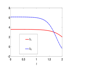
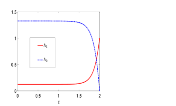
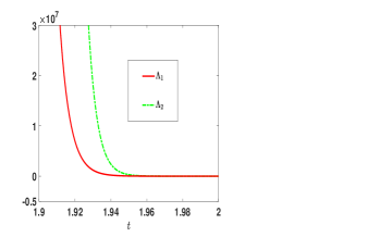
Figure 1. Solvability of $(\Lambda_{1},\Lambda_{2})$ on $[0,T]$ with $T=2$. Left panel: Example 1 with $R>0$. Middle panel: Example 2 with $R<0$. Right panel: Example 3.

6.2. Performance

To numerically compare $J_{\rm soc}^{(N)}(U^{o})$ and $J_{\rm soc}^{(N)}({U}^{d})$, we need to solve the system (3.18) for $(\Lambda_{1}^{N},\Lambda_{2}^{N})$ associated with the centralized control $U^{o}$ and next the system (5.16)–(5.19) for $(\check{\Lambda}_{1}^{N},\check{\Lambda}_{2}^{N},\check{\Lambda}_{12}^{N},\check{\Lambda}_{22}^{N})$ associated with the decentralized control $U^{d}$. By Theorem 3.1, if the Riccati ODE system consisting of (3.7) and (3.37) has a solution on $[0,T]$, then (3.18) has a solution on $[0,T]$ for all sufficiently large $N$, and so does the system (5.16)–(5.19).

Recall the necessary and sufficient condition in Section 3.2 for the solvability of (3.7) and (3.37). We will take $Q$, $Q_{f}\geq 0$, and $R>0$, under which (3.7) and (3.37) have a unique solution on $[0,T]$ [65, Theorem 6.7.2]. With the same parameter values as in Example 1, we numerically solve the systems (3.18), (3.7)–(3.8), and (5.16)–(5.19). The initial conditions are given as $X_{i}(0)=1$ for all $i\geq 1$, and $\overline{X}(0)=1$.

Fig. 2 (left panel) shows that the difference ($\check{\Lambda}_{12}^{N}=\check{\Lambda}_{12}^{NT}$ for the scalar case)

$$[\check{\Lambda}_{1}^{N}(0)+\check{\Lambda}_{2}^{N}(0)+\check{\Lambda}_{12}^{N}(0)+\check{\Lambda}_{12}^{NT}(0)+\check{\Lambda}_{22}^{N}(0)]-[\Lambda_{1}^{N}(0)+\Lambda_{2}^{N}(0)]$$

approaches $0$ as $N\to\infty$, as asserted by Lemma 5.5. Fig. 2 (right panel) shows that the difference $J_{\rm soc}^{(N)}({U}^{d})-J_{\rm soc}^{(N)}(U^{o})$ remains bounded as $N$ increases.

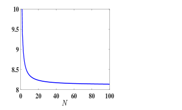
Figure 2. Left panel: The difference $\check{\Lambda}_{1}^{N}+\check{\Lambda}_{2}^{N}+\check{\Lambda}_{12}^{N}+\check{\Lambda}_{12}^{NT}+\check{\Lambda}_{22}^{N}-(\Lambda_{1}^{N}+\Lambda_{2}^{N})$ evaluated at $t=0$ for $N\geq 1$. Right panel: The difference $J_{\rm soc}^{(N)}({U}^{d})-J_{\rm soc}^{(N)}(U^{o})$ for $N\geq 1$.

6.3. Comparison between the social optimum and the mean field equilibrium

We use the model in Example  1 to compare the per agent costs $\bar{J}_{i,{\rm soc}}$ and $\bar{J}_{i,{\rm mfg}}$ for social optimization and the mean field game, respectively. The initial states $X_{i}(0)$ have mean $\mu_{0}$ and variance $\Sigma_{0}$.

Fig. 3 compares $\Lambda_{1}^{g}+\Lambda_{2}^{g}+\Lambda_{2}^{gT}+\Lambda_{4}^{g}$ and $\Lambda_{3}$ on $[0,T]$ ($\Lambda_{2}^{g}=\Lambda_{2}^{gT}$ for the scalar case). Note that $\Lambda_{3}=\Lambda_{1}+\Lambda_{2}$ on $[0,T]$. Since

$$\bar{J}_{i,{\rm mfg}}-\bar{J}_{i,{\rm soc}}=(\Lambda_{1}^{g}(0)+\Lambda_{2}^{g}(0)+\Lambda_{2}^{gT}(0)+\Lambda_{4}^{g}(0)-\Lambda_{3}(0))\mu_{0}^{2},$$

Fig. 3 confirms that the per agent cost of the social optimal control is lower than that of the mean field equilibrium strategy.

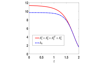
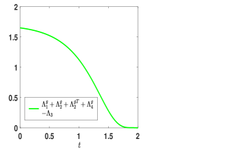
Figure 3. Left panel: Comparison between $\Lambda_{1}^{g}+\Lambda_{2}^{g}+\Lambda_{2}^{gT}+\Lambda_{4}^{g}$ and $\Lambda_{3}$. Right panel: The difference $\Lambda_{1}^{g}+\Lambda_{2}^{g}+\Lambda_{2}^{gT}+\Lambda_{4}^{g}-\Lambda_{3}$.

7. Conclusion

This paper studies asymptotic solvability for LQ mean field social optimization problems with indefinite state and control weight matrices. The analysis involves highly nonlinear large-scale Riccati ODEs due to controlled diffusions. We derive a necessary and sufficient condition for asymptotic solvability. We obtain a set of decentralized individual control laws, and further show that its optimality loss is bounded. We further check the efficiency gain of the social optimal control with respect to the mean field game.

Appendix A Proof of Lemma 3.1

Proof.

Write the $Nn\times Nn$ identity matrix $I_{Nn}$ as $I_{Nn}=\operatorname{diag}[I_{n},I_{n},\cdots,I_{n}]$. Let $J_{ij}$ denote the matrix obtained by exchanging the $i$th and $j$th rows of the submatrices in $I_{Nn}$. It is easy to check that $J_{ij}=J_{ji}$ and $J_{ij}=J_{ij}^{T}=J_{ij}^{-1}$ for all $i,j$.

Denote $\mathbf{P}=(P_{ij})_{1\leq i,j\leq N}$, where each $P_{ij}$ is an $n\times n$ matrix. We choose arbitrary $i\neq j$, and denote $J^{T}_{ij}\mathbf{P}J_{ij}=\mathbf{P}^{\dagger}_{(ij)}$. In this proof we write $\mathbf{P}_{(ij)}^{\dagger}$ as $\mathbf{P}^{\dagger}$ for simplicity of notation. We multiply both sides of (2.8) from the left by $J_{ij}^{T}$ and next from the right by $J_{ij}$ to get

$$\dot{\mathbf{P}}^{\dagger}(t)=\mathbf{P}^{\dagger}\widehat{\mathbf{B}}\left(\mathbf{R}+2\mathcal{M}_{2}(\mathbf{P}^{\dagger})\right)^{-1}\widehat{\mathbf{B}}^{T}\mathbf{P}^{\dagger}-\mathbf{P}^{\dagger}\mathbf{A}-\mathbf{A}^{T}\mathbf{P}^{\dagger}-\mathbf{Q},$$

where we use the following facts with $\Psi=\mathbf{A}$, $\widehat{\mathbf{B}}$, $\mathbf{R}$, or $\mathbf{Q}$,

$$J_{ij}^{T}(\mathbf{B}_{k}\mathbf{e}_{k})J_{ij}=\begin{cases}\mathbf{B}_{k}\mathbf{e}_{k}&\text{if}\ k\neq i,j,\\ \mathbf{B}_{j}\mathbf{e}_{j}&\text{if}\ k=i,\\ \mathbf{B}_{i}\mathbf{e}_{i}&\text{if}\ k=j,\end{cases}\quad\text{and}\quad J_{ij}^{T}\Psi J_{ij}=\Psi.$$

Thus $\mathbf{P}^{\dagger}$ also satisfies (2.8). It then follows that $J_{ij}^{T}\mathbf{P}J_{ij}=\mathbf{P}$ for any $i\neq j$, and the matrix $\mathbf{P}=(P_{ij})_{1\leq i,j\leq N}$ satisfies that

$$P_{ii}=P_{jj},\quad P_{ij}=P_{ji},\quad P_{ik}=P_{jk},\quad P_{ki}=P_{kj},\quad\forall k\neq i,j.$$

This implies that the diagonal submatrices $\{P_{ii},{1\leq i\leq N}\}$ are equal and all the off-diagonal submatrices $\{P_{ij},{1\leq i\neq j\leq N}\}$ are equal. Since $\mathbf{P}$ is symmetric, now $P_{ij}=P_{ji}^{T}=P_{ji}$ for all $i\neq j$. We denote $P_{ii}=\Pi_{1}^{N}$ for all $1\leq i\leq N$, and $P_{ij}=\Pi_{2}^{N}$ for all $1\leq i\neq j\leq N$. Then (3.9) follows. ∎

Appendix B Proof of Lemmas 3.2 and 3.4

Proof of Lemma 3.2.

Existence and uniqueness holds since (2.9) is a linear ODE. The remaining proof is similar to that of Lemma 3.1. We multiply both sides of the ODE (2.9) from the left by $J_{ij}$ as in the proof of Lemma 3.1 so that

$$J_{ij}\dot{\mathbf{S}}(t) =\mathbf{P}\widehat{\mathbf{B}}(\mathbf{R}+2\mathcal{M}_{2}(\mathbf{P}))^{-1}(\widehat{\mathbf{B}}^{T}J_{ij}\mathbf{S}+\mathcal{M}_{1}^{T}(\mathbf{P}))-\mathbf{A}^{T}J_{ij}\mathbf{S}.$$

Since $J_{ij}\mathbf{S}$ and $\mathbf{S}$ satisfy the same ODE, for arbitrary $i\neq j$, we conclude that $\mathbf{S}$ takes the form (3.10). ∎

Proof of Lemma 3.4.

Let $J_{ij}$ be the matrix as defined in the proof of Lemma 3.1. Multiplying both sides of the identity

$$I=(\mathbf{R}+2\mathcal{M}_{2}(\mathbf{P}))(\mathbf{R}+2\mathcal{M}_{2}(\mathbf{P}))^{-1}$$

from the left by $J_{ij}^{T}$ and next from the right by $J_{ij}$, for $1\leq i\neq j\leq N$, we obtain

$$I =J_{ij}^{T}(\mathbf{R}+2\mathcal{M}_{2}(\mathbf{P}))(\mathbf{R}+2\mathcal{M}_{2}(\mathbf{P}))^{-1}J_{ij}$$

$$=J_{ij}^{T}(\mathbf{R}+2\mathcal{M}_{2}(\mathbf{P}))J_{ij}J_{ij}^{T}(\mathbf{R}+2\mathcal{M}_{2}(\mathbf{P}))^{-1}J_{ij}.$$

Since $J_{ij}^{T}(\mathbf{R}+2\mathcal{M}_{2}(\mathbf{P}))J_{ij}=\mathbf{R}+2\mathcal{M}_{2}(\mathbf{P})$, it follows that $J_{ij}^{T}(\mathbf{R}+2\mathcal{M}_{2}(\mathbf{P}))^{-1}J_{ij}=(\mathbf{R}+2\mathcal{M}_{2}(\mathbf{P}))^{-1}$, and thus $E^{NT}=E^{N}$. ∎

Appendix C Mean field game ODEs

The ODEs of $(\Lambda_{1}^{g},\Lambda_{2}^{g},\Lambda_{3}^{g},\Lambda_{4}^{g})$ corresponding to the mean field game in Section 5.3 are given as follows:

$$\begin{cases}\dot{\Lambda}_{1}^{g}=\Psi_{1}(\Lambda_{1}^{g}),\\ \Lambda_{1}^{g}(T)=Q_{f},\ \mathcal{R}_{1}(\Lambda_{1}^{g}(t))>0,\ \forall t\in[0,T],\end{cases}$$

$$\begin{cases}\dot{\Lambda}_{2}^{g}=\Lambda_{2}^{g}BH^{g}B^{T}\Lambda_{2}^{g}+\Lambda_{2}^{g}BH^{g}B^{T}\Lambda_{1}^{g}+\Lambda_{1}^{g}BH^{g}B^{T}\Lambda_{2}^{g}\\ \hskip 22.76228pt-\Lambda_{1}^{g}G-\Lambda_{2}^{g}(A+G)-A^{T}\Lambda_{2}^{g}+Q\Gamma,\\ \Lambda_{2}^{g}(T)=-Q_{f}\Gamma_{f},\end{cases}$$

$$\begin{cases}\dot{\Lambda}_{3}^{g}=\Lambda_{3}^{g}BH^{g}B^{T}\Lambda_{1}^{g}+\Lambda_{1}^{g}BH^{g}B^{T}\Lambda_{3}^{g}+\Lambda_{4}^{g}BH^{g}B^{T}\Lambda_{2}^{g}\\ \hskip 22.76228pt+\Lambda_{2}^{gT}BH^{g}B^{T}(\Lambda_{2}^{g}+\Lambda_{4}^{g})-\Lambda_{1}^{g}BH^{g}B_{1}^{T}\Lambda_{3}^{g}B_{1}H^{g}B^{T}\Lambda_{1}^{g}\\ \hskip 22.76228pt-(\Lambda_{1}^{g}+\Lambda_{2}^{gT})BH^{g}B_{0}^{T}(\Lambda_{1}^{g}+\Lambda_{2}^{g}+\Lambda_{2}^{gT}+\Lambda_{4}^{g})B_{0}H^{g}B^{T}(\Lambda_{1}^{g}+\Lambda_{2}^{g})\\ \hskip 22.76228pt-\Lambda_{3}^{g}A-(\Lambda_{2}^{gT}+\Lambda_{4}^{gT})G-A^{T}\Lambda_{3}^{g}-G^{T}(\Lambda_{2}^{g}+\Lambda_{4}^{g})-\Gamma^{T}Q\Gamma,\\ \Lambda_{3}^{g}(T)=\Gamma_{f}^{T}Q_{f}\Gamma_{f},\end{cases}$$

$$\begin{cases}\dot{\Lambda}_{4}^{g}=\Lambda_{4}^{g}BH^{g}B^{T}(\Lambda_{1}^{g}+\Lambda_{2}^{g})+\Lambda_{1}^{g}BH^{g}B^{T}\Lambda_{4}^{g}+\Lambda_{2}^{gT}BH^{g}B^{T}(\Lambda_{2}^{g}+\Lambda_{4}^{g})\\ \hskip 22.76228pt-(\Lambda_{1}^{g}+\Lambda_{2}^{gT})BH^{g}B_{0}^{T}(\Lambda_{1}^{g}+\Lambda_{2}^{g}+\Lambda_{2}^{gT}+\Lambda_{4}^{g})B_{0}H^{g}B^{T}(\Lambda_{1}^{g}+\Lambda_{2}^{g})\\ \hskip 22.76228pt-(\Lambda_{2}^{gT}+\Lambda_{4}^{g})G-\Lambda_{4}^{g}A-G^{T}(\Lambda_{2}^{g}+\Lambda_{4}^{g})-A^{T}\Lambda_{4}^{g}-\Gamma^{T}Q\Gamma,\\ \Lambda_{4}^{g}(T)=\Gamma_{f}^{T}Q_{f}\Gamma_{f},\end{cases}$$

where we use the notation $H^{g}=(\mathcal{R}_{1}(\Lambda_{1}^{g}))^{-1}$.

References

- [1] G. Albi, Y.-P. Choi, M. Fornasier, and D. Kalise. Mean field control hierarchy. Appl. Math. Optim., 76(1):93–135, 2017.
- [2] D. Andersson and B. Djehiche. A maximum principle for SDEs of mean-field type. Appl. Math. Optim., 63:341–356, 2011.
- [3] J. Arabneydi and A. Mahajan. Team-optimal solution of finite number of mean-field coupled LQG subsystems. In Proc. 54th IEEE CDC, pages 5308–5313, Osaka, Japan, Dec. 2015.
- [4] J. Arabneydi and A. Mahajan. Linear quadratic mean field teams: Optimal and approximately optimal decentralized solutions. arXiv:1609.00056, 2017.
- [5] M. Bardi and F. S. Priuli. Linear-quadratic -person and mean-field games with ergodic cost. SIAM J. Control Optim., 52(5):3022–3052, 2014.
- [6] E. Bayraktar, A. Cosso, and H. Pham. Randomized dynamic programming principle and Feynman–Kac representation for optimal control of McKean–Vlasov dynamics. Trans. Amer. Math. Soc., 370(3):2115–2160, 2018.
- [7] A. Bensoussan, J. Frehse, and S. C. P. Yam. Mean Field Games and Mean Field Type Control Theory. Springer, New York, 2013.
- [8] A. Bensoussan, J. Frehse, and S. C. P. Yam. The master equation in mean field theory. Journal de Mathématiques Pures et Appliquées, 103(6):1441–1474, 2015.
- [9] A. Bensoussan, K. C. J. Sung, S. C. P. Yam, and S. P. Yung. Linear-quadratic mean-field games. J. Optim. Theory Appl., 169(2):496–529, 2016.
- [10] R. Buckdahn, J. Li, and J. Ma. A stochastic maximum principle for general mean-field systems. Appl. Math. Optim., 74:507–534, 2016.
- [11] P. E. Caines, M. Huang, and R. P. Malhamé. Mean field games. In T. Başar and G. Zaccour, editors, Handbook of Dynamic Game Theory, pages 345–372. Springer, Berlin, 2017.
- [12] P. Cardaliaguet. Notes on mean field games. University of Paris, Dauphine, 2013.
- [13] P. Cardaliaguet, F. Delarue, J.-M. Lasry, and P.-L. Lions. The master equation and the convergence problem in mean field games. arXiv:1509.02505, 2015.
- [14] P. Cardaliaguet and C. Rainer. On the (in)efficiency of MFG equilibria. SIAM J. Control Optim., 57(4):2292–2314, 2019.
- [15] R. Carmona and F. Delarue. Probabilistic Theory of Mean Field Games with Applications I-II. Springer, Cham, Switzerland, 2018.
- [16] R. Carmona, F. Delarue, and A. Lachapelle. Control of McKean–Vlasov dynamics versus mean field games. Math. Financial Econ., 7(2):131–166, 2013.
- [17] P. Chan and R. Sircar. Bertrand and Cournot mean field games. Appl. Math. Optim., 71:533–569, 2015.
- [18] S. Chen, X. Li, and X. Y. Zhou. Stochastic linear quadratic regulators with indefinite control weight costs. SIAM J. Control Optim., 36(5):1685–1702, 1998.
- [19] X. Chen and M. Huang. Linear-quadratic mean field control: the Hamiltonian matrix and invariant subspace method. In Proc. 57th IEEE CDC, pages 4117–4122, Miami Beach, FL, Dec. 2018.
- [20] X. Chen and M. Huang. Linear-quadratic mean field control: the invariant subspace method. Automatica, 107:582–586, Sep. 2019.
- [21] M. Chiang, S. H. Low, A. R. Calderbank, and J. C. Doyle. Layering as optimization decomposition: A mathematical theory of network architectures. Proceedings of the IEEE, 95(1):255–312, 2007.
- [22] F. M. Djete, D. Possamaï, and X. Tan. McKean–Vlasov optimal control: limit theory and equivalence between different formulations. arXiv:2001.00925, 2020.
- [23] R. Elliott, X. Li, and Y.-H. Ni. Discrete time mean-field stochastic linear-quadratic optimal control problems. Automatica, 49(11):3222–3233, Nov. 2013.
- [24] J. Engwerda. Necessary and sufficient conditions for Pareto optimal solutions of cooperative differential games. SIAM J. Control Optim., 48(6):3859–3881, 2010.
- [25] A. Ferrante and L. Ntogramatzidis. A note on finite-horizon LQ problems with indefinite cost. Automatica, 52:290–293, Feb. 2015.
- [26] M. Fischer and G. Livieri. Continuous time mean-variance portfolio optimization through the mean field approach. ESAIM: P&S, 20:30–44, 2016.
- [27] M. Fornasier and F. Solombrino. Mean-field optimal control. ESAIM: COCV, 20(4):1123–1152, 2014.
- [28] D. A. Gomes and J. Saude. Mean field games models: A brief survey. Dyn. Games Appl., 4:110–154, 2014.
- [29] P. J. Graber. Linear quadratic mean field type control and mean field games with common noise, with application to production of an exhaustible resource. Appl. Math. Optim., 74:459–486, 2016.
- [30] O. Guéant, J.-M. Lasry, and P.-L. Lions. Mean field games and applications. In Paris-Princeton Lectures on Mathematical Finance, pages 205–266. Springer-Verlag, Berlin, Heidelberg, 2011.
- [31] M. H. Hajiesmaili, M. S. Talebi, and A. Khonsari. Multiperiod network rate allocation with end-to-end delay constraints. IEEE Trans. Control Netw. Syst., 5(3):1087–1097, 2017.
- [32] J. Huang, S. Wang, and Z. Wu. Backward mean-field linear-quadratic-Gaussian (LQG) games: Full and partial information. IEEE Trans. Autom. Control, 61(12):3784–3796, Dec. 2016.
- [33] M. Huang, P. E. Caines, and R. P. Malhamé. Large-population cost-coupled LQG problems with non-uniform agents: Individual-mass behavior and decentralized -Nash equilibria. IEEE Trans. Autom. Control, 52(9):1560–1571, Sep. 2007.
- [34] M. Huang, P. E. Caines, and R. P. Malhamé. Social optima in mean field LQG control: Centralized and decentralized strategies. IEEE Trans. Autom. Control, 57(7):1736–1751, 2012.
- [35] M. Huang, R. P. Malhamé, and P. E. Caines. Large population stochastic dynamic games: Closed-loop McKean-Vlasov systems and the Nash certainty equivalence principle. Commun. Inform. Systems, 6(3):221–252, 2006.
- [36] M. Huang and X. Yang. Linear quadratic mean field social optimization: Asymptotic solvability. In Proc. 58th IEEE CDC, pages 8210–8215, Nice, France, Dec. 2019.
- [37] M. Huang and X. Yang. Linear quadratic mean field games: Decentralized -Nash equilibria. Journal of Systems Science and Complexity, 2021. to appear.
- [38] M. Huang and M. Zhou. Linear quadratic mean field games–part i: the asymptotic solvability problem. In Proc. 23rd Internat. Symp. Math. Theory Networks and Systems, pages 489–495, Hong Kong, China, July 2018.
- [39] M. Huang and M. Zhou. Linear quadratic mean field games: Asymptotic solvability and relation to the fixed point approach. IEEE Trans. Autom. Control, 65(4):1397–1412, April 2020.
- [40] F. P. Kelly, A. K. Maulloo, and D. K. Tan. Rate control for communication networks: shadow prices, proportional fairness and stability. J. Oper. Res. Soc., 49(3):237–252, 1998.
- [41] D. Lacker. Limit theory for controlled McKean–Vlasov dynamics. SIAM J. Control Optim., 55(3):1641–1672, 2017.
- [42] J.-M. Lasry and P.-L. Lions. Mean field games. Japan. J. Math., 2(1):229–260, 2007.
- [43] S. Li, W. Zhang, and L. Zhao. Connections between mean-field game and social welfare optimization. Automatica, 110:108590, 2019.
- [44] Y. Ma and M. Huang. Linear quadratic mean field games with a major player: The multi-scale approach. Automatica, 113(3), 2020.
- [45] A. Mas-Colell, M. D. Whinston, and J. R. Green. Microeconomic Theory. Oxford University Press, Oxford, 1995.
- [46] J. Moon and T. Başar. Linear quadratic risk-sensitive and robust mean field games. IEEE Trans. Autom. Control, 62(3):1062–1077, 2017.
- [47] H. Moulin. Fair Division and Collective Welfare. MIT press, 2004.
- [48] Y.-H. Ni, J.-F. Zhang, and X. Li. Indefinite mean-field stochastic linear-quadratic optimal control. IEEE Trans. Autom. Control, 60(7):1786–1800, July 2015.
- [49] G. Nuño and B. Moll. Social optima in economies with heterogeneous agents. Rev. Econ. Dyn., 28:150–180, April 2018.
- [50] H. Pham. Continuous-time stochastic control and optimization with financial applications. Springer Science & Business Media, Berlin, 2009.
- [51] H. Pham. Linear quadratic optimal control of conditional Mckean–Vlasov equation with random coefficients and applications. Probability, Uncertainty and Quantitative Risk, 1(1):1–26, 2016.
- [52] H. Pham and X. Wei. Dynamic programming for optimal control of stochastic McKean–Vlasov dynamics. SIAM J. Control Optim., 55(2):1069–1101, 2017.
- [53] M. A. Rami, X. Chen, and X. Y. Zhou. Discrete-time indefinite LQ control with state and control dependent noises. J. Global Optim., 23:245–265, 2002.
- [54] M. A. Rami, J. B. Moore, and X. Y. Zhou. Indefinite stochastic linear quadratic control and generalized differential Riccati equation. SIAM J. Control Optim., 40(4):1296–1311, 2001.
- [55] R. Salhab, R. P. Malhamé, and J. L. Ny. A dynamic game model of collective choice in multiagent systems. IEEE Trans. Autom. Control, 63(3):768–782, Mar. 2018.
- [56] R. Salhab, J. L. Ny, and R. P. Malhamé. Dynamic collective choice: Social optima. IEEE Trans. Autom. Control, 63(10):3487–3494, Oct. 2018.
- [57] S. S. Sanjari and S. Yuksel. Optimal solutions to infinite-player stochastic teams and mean-field teams. IEEE Trans. Autom. Control, 66(3):1071–1086, 2021.
- [58] N. Sen, M. Huang, and R. P. Malhamé. Mean field social control with decentralized strategies and optimality characterization. In Proc. 55th IEEE CDC, pages 6056–6061, Las Vegas, NV, Dec. 2016.
- [59] J. Sun, X. Li, and J. Yong. Open-loop and closed-loop solvabilities for stochastic linear quadratic optimal control problems. SIAM J. Control Optim., 54(5):2274–2308, 2016.
- [60] N. Trichakis, A. Zymnis, and S. Boyd. Dynamic network utility maximization with delivery contracts. IFAC Proceedings Volumes, 41(2):2907–2912, 2008.
- [61] B.-C. Wang and J.-F. Zhang. Social optima in mean field linear-quadratic-Gaussian models with Markov jump parameters. SIAM J. Control Optim., 55(1):429–456, 2017.
- [62] W. M. Wonham. On a matrix Riccati equation of stochastic control. SIAM J. Control, 6(4):681–697, 1968.
- [63] Y. Wu, J. Wu, M. Huang, and L. Shi. Mean-field transmission power control in dense networks. IEEE Trans. Control Netw. Syst., 8(1):99–110, 2021.
- [64] J. Yong. Linear-quadratic optimal control problems for mean-field stochastic differential equations. SIAM J. Control Optim., 51(4):2809–2838, 2013.
- [65] J. Yong and X. Y. Zhou. Stochastic Controls: Hamiltonian Systems and HJB Equations. Springer-Verlag, New York, 1999.
- [66] K. Yosida. Functional Analysis. Springer-Verlag, Berlin, 6th edition, 1980.
- [67] X. Y. Zhou and D. Li. Continuous-time mean-variance portfolio selection: A stochastic LQ framework. Appl. Math. Optim., 42(1):19–33, 2000.