Audio-Visual Floorplan Reconstruction
Abstract
Given only a few glimpses of an environment, how much can we infer about its entire floorplan? Existing methods can map only what is visible or immediately apparent from context, and thus require substantial movements through a space to fully map it. We explore how both audio and visual sensing together can provide rapid floorplan reconstruction from limited viewpoints. Audio not only helps sense geometry outside the camera’s field of view, but it also reveals the existence of distant freespace (e.g., a dog barking in another room) and suggests the presence of rooms not visible to the camera (e.g., a dishwasher humming in what must be the kitchen to the left). We introduce AV-Map, a novel multi-modal encoder-decoder framework that reasons jointly about audio and vision to reconstruct a floorplan from a short input video sequence. We train our model to predict both the interior structure of the environment and the associated rooms’ semantic labels. Our results on 85 large real-world environments show the impact: with just a few glimpses spanning 26% of an area, we can estimate the whole area with 66% accuracy — substantially better than the state of the art approach for extrapolating visual maps.
1 Introduction
Floorplans of complex 3D environments—such as homes, offices, shops, churches—are a compact ground-plane representation of their overall layout, showing the different rooms and their connectivity. Floorplans are useful for visualizing a large space, navigating an unfamiliar building, planning safety routes, and communicating architectural designs. In robotics, an agent entering a new building needs to quickly sense the overall layout, but without visiting every part of it.
Traditionally a floorplan is created by distilling a fully observed 3D environment into its footprint—whether manually or with the aid of 3D sensors [41, 30]. Recent research aims to infer room layouts using imagery and/or scans, with impressive results [28, 8, 26, 45]. However, existing methods are limited to mapping the regions they directly observe. They either require a dense walk-through for the camera to capture most of the space—wasteful if not impossible for a robotic agent trying to immediately perform tasks in a new environment—or else they simply fail to map rooms beyond those where the camera was placed.
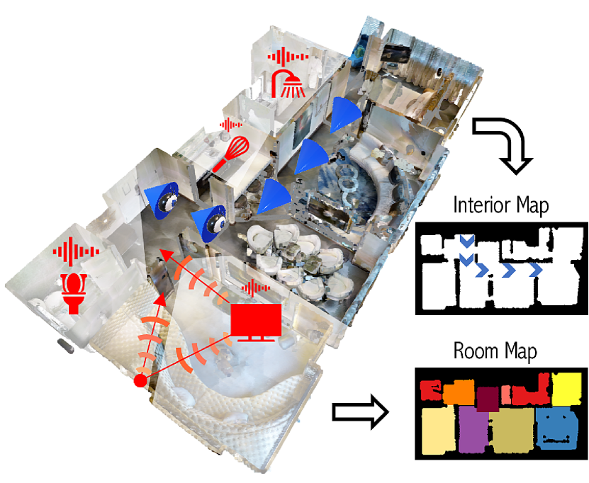
Our idea is to “see" beyond the visible regions by listening. Audio provides strong spatial and semantic signals that complement the mapping capabilities of visual sensing. In particular, the value of audio for floorplan estimation is threefold. First, observed sound is inherently driven by geometry; audio reflections bounce off major surfaces and reveal the shape of a room, beyond the camera’s field of view. Second, sounds heard from afar—even multiple rooms away—can suggest the existence of distant freespace where the sounding object could exist (e.g., a dog barking in another room). Third, hearing semantically meaningful sounds from different directions naturally reveals the plausible room layouts based on the activities or objects those sounds represent. For example, a shower running suggests the direction of the bathroom, even before we see it; microwave beeps suggest a kitchen; climbing footsteps suggest a staircase. See Figure 1.
To this end, we propose a new research direction: audio-visual floorplan reconstruction. Given a short RGB video complete with multi-channel audio, the goal is to produce a 2D floorplan that shows the freespace and occupied regions and divides them into a discrete set of semantic room labels (family room, kitchen, etc.). Importantly, the floorplan output extends significantly beyond the area directly observable in the video frames. This efficiency is critical for navigating robots that need to act without exhaustively touring a space, as well as offline scenarios where a user wants to extract a broad map from an existing short video.
Our AV-Map approach works as follows. We devise a deep convolutional neural network architecture that leverages sequences of audio and visual data to reason about the structure and semantics of the floorplan. Our model independently extracts floorplan-aligned features for audio and RGB data, encodes sequences of features of each modality using self-attention mechanisms, and finally fuses information from audio and RGB using a decoder architecture.
We consider two settings: device-generated sounds (active) and environment-generated sounds (passive). In the active setting, the camera emits a known sound while it moves. This corresponds to a use case where a person or robot does a swift walk-through of an environment while their phone/camera emits some sound. In the passive setting, we observe only naturally occurring sounds made by objects and people in the building. This corresponds to a use case where we are simply given a passively recorded video, likely captured for some other purpose.
To our knowledge, ours is the first attempt to infer floorplans from audio-visual data. Our results on 85 large real-world, multi-room environments show that AV-Map not only consistently outperforms traditional vision-based mapping, but also improves the state-of-the-art approach [33] for extrapolating occupancy maps beyond visible regions (with a relative gain of 8% in floorplan accuracy). Though observing only a small fraction of the full homes, our model yields good interior maps covering much of their area. We also show audio and vision are synergistic signals to classify room types, allowing high-level perception of the semantics of the space even before directly visiting each room.
2 Related Work
Floorplan and room layout reconstruction
The vision and graphics communities have explored various ways to use visual data, depth sensors, and laser scanners to build floorplans. Geometric approaches use 3D point cloud inputs to construct building-wide floor plans [41, 30]. Given RGB-D scans, FloorNet [28] and Floor-SP [8] estimate 2D floorplans and rooms’ semantic labels using a mix of deep learning and optimization. Given monocular RGB images [26] or panoramas [45, 48, 42, 49], other methods estimate a 3D indoor Manhattan room layout. Using only a small portion of a panorama, models can be trained to infer missing viewpoints [22] and/or semantic labels [39]. Unlike any of the above, our approach leverages both audio and visual sensing to infer a 2D floorplan map and its semantic room labels. As our results show, audio offers the advantage of sensing further beyond the field of view of visual sensors.
Mapping for navigation
With adequate overlapping views, structure-from-motion methods can recover the 3D structure of an environment (e.g., [2, 37]). Laser-based 2D SLAM is often used in mobile robotics to obtain the ground plane map [34]. Recent work leverages scans of indoor environments [3, 40] and fast simulation tools [36] to facilitate work on embodied visual navigation [20, 35, 24, 4, 9, 33]. While often the map is implicitly learned, some methods explicitly estimate a 2D occupancy map, projecting the observed point cloud to the ground plane and growing the map over time [9, 33, 4]. To navigate to a specified room, the method of [29] predicts a 2D semantic map with room labels, learning the layout patterns in houses. In contrast to navigation, where an intelligent agent controls the camera and builds its map in service of reaching a target, our goal is to transform a passive video sequence (with audio) into a map. We show the advantages of our audio-visual approach over OccAnt [33], the state-of-the-art navigation method that extrapolates beyond visible scene points using vision alone.
Audio for spatial sensing
Prior work explores ways to exploit audio alone to sense the shape of a room or object. Given multiple microphone recordings of a known sound, the method of [13] computes the shape of a single convex polyhedral room, while sound reflections are used to sense the 3D shape of an object hidden around a corner [27]. In robotics, echolocation can detect distances to surfaces based on the reflections [38, 14, 44, 10]. Multi-channel audio is also used to track dynamic objects [11, 16]. Unlike any of these methods, our approach takes a video (both the audio and visual streams) as input and produces a floorplan as output. Furthermore, our model is not restricted to known microphone layouts or known emitted sounds; rather, it can learn from natural sounds sensed passively in the environment (e.g., running water, door shutting). While environment semantics are explored in acoustic scene analysis [18, 19], our problem is quite different: the target output is a geometric map, not a label for the acoustic event that occurred.
Audio-visual spatial sensing
Audio and vision together offer powerful cues for spatial perception. At the object level, they reveal shape and material properties [47, 31], e.g., via the sound of one object striking another. At the environment level, audio can help sense 3D surfaces in cases where depth sensing would fail, e.g., transparent, shiny, or textureless surfaces [46, 25], or provide self-supervisory cues for imagery [17]. Recent work leverages audio-visual sensing to address navigation tasks, learning to move efficiently to a sounding target [5, 15, 7]. In [12], a curiosity-driven framework is proposed that leverages audio-visual cues to explore environments. None of the above methods produce audio-visual floorplans. Furthermore, an insight unique to our work is the use of naturally occurring semantic sounds to understand a multi-room layout.
3 Approach
Our goal is to estimate the 2D layout of an environment depicted in a short video. The 2D layout has two components: the structure of the interior area, and the semantic labels (room types) associated with each region of the interior. First, we formally describe the problem (Sec 3.1). We then describe our proposed model AV-Map (Sec 3.2) and introduce our training and inference procedure (Sec 3.3).
3.1 Problem Formulation
We consider videos generated by a camera and an ambisonic microphone following short trajectories through various home environments. An ambisonic mic captures omni-directional multi-channel audio [1, 32]. We represent a video by where is the RGB frame and is the audio clip sampled at time step . Additionally, let us denote by the position of the camera and microphone relative to the first time step in the coordinate system of the floorplan, where represents the movement along the x- and y-axis on the 2D ground plane and represents the rotation about the gravity axis. Relative pose changes in a video can be estimated using computer vision [21]; for simplicity we assume correct relative camera poses are available for all methods. However, we find our proposed model is robust to noise in pose estimation within the range of odometry noise models considered in the literature [33], owing to the resolution of the output floorplan.
Each floorplan is parameterized as two variables: and , which represent the structure and semantics, respectively. The interior map is a 2D binary grid that is a top-down view of the environment and represents the existence of floor, objects, furniture by label , and walls and areas outside the environment by label . The room map is a 2D grid taking possible values with labels representing the room types (kitchen, bathroom, etc.) and representing walls and areas outside the environment. Each cell in the floorplan (an entry in the matrix ) represents a 25cm2 area.
The goal of our work is to learn a mapping that estimates the floorplan (both and ) of an environment using the video and the relative pose changes . The visual information in captures the geometric properties and room types of visible regions. The audio information captured in is either actively emitted by the camera, or else passively generated by objects and people in the environment (details below). Since the placement of objects is highly correlated with room types (for example, showers are in bathrooms and dishwashers are in kitchens), the audio signal captures a strong semantic signal indicating the room types. Furthermore, the echoes propagating through the environment capture geometric properties of the walls and other major surfaces. Our key insight is that the audio observations will illuminate the map for regions beyond what is visible in the frames of a short video.
3.2 AV-Map Floorplan Estimation Model
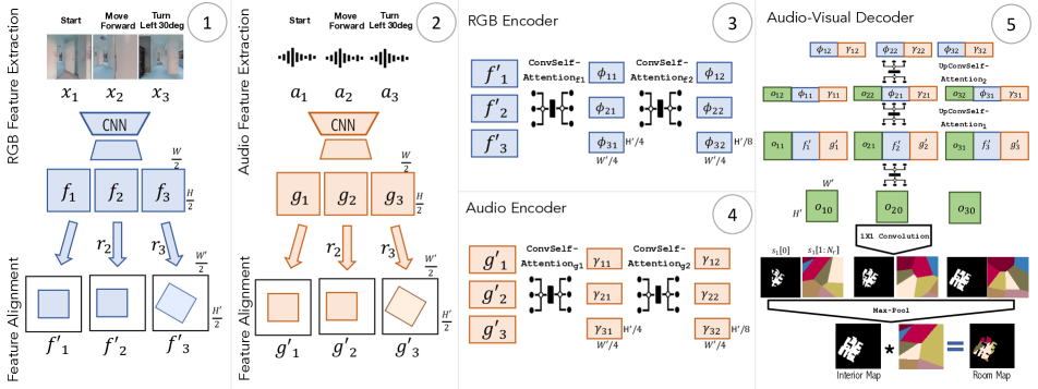
We now present our AV-Map floorplan estimation model . Fig. 2 overviews our proposed model, consisting of three components: Top-Down Feature Extraction, Feature Alignment, and a Sequence Encoder-Decoder architecture. At each time step, AV-Map estimates the interior map () and semantic room labels () in a neighborhood centered around the camera, integrating estimates over time.
Top-Down Feature Extraction
The first stage of our proposed model involves extracting features for a given video . The purpose of the feature extraction step is to project egocentric visual frames and ambisonic audio clips to a 2D feature grid that is spatially aligned with the top-down floorplan that we wish to estimate at each time step.
RGB Feature Extraction The feature extractor for an RGB frame consists of a ResNet-18 model up to layer2 followed by a spatial pooling operation, which leads to a single 128-D feature. We use layer2 features of the ResNet to capture low-level features like corners of rooms. This feature is then upsampled by a sequence of transposed convolutions leading to the final visual feature where are the height and width of the considered output floorplan area at each time step. See Fig. 2, Column 1. Importantly, this predicted area extends beyond the freespace directly observable from the visual frame ; in our experiments, the visually observed space on average covers only 13.7% of the area in when comprises of 40m2 around the camera. Below we explain how maps from multiple steps are aggregated for the video’s final (larger) output map.
Audio Feature Extraction A video also consists of audio clips where is the sound duration at each time step , and is the number of ambisonic channels corresponding to second order ambisonics. Features for each audio clip are extracted using a sequence of linear, ReLU, and pooling layers, yielding a 128-D feature. Similar to the RGB extractor, this feature is upsampled via transposed convolutions to obtain the final audio feature . See Fig. 2, Column 2.
Feature Alignment
After extracting features for the RGB frames and audio clips, each video is represented by the set of visual features and audio features , for , where is the number of frames in video and may vary across videos. Note that each of these features was computed independently and thus far represents a feature aligned with the top-down map in a canonical frame-centric coordinate frame. In order to process entire sequences, we need to establish correspondences between the features at each time step. Therefore, we next align all the features to a common coordinate system, relative to the first frame. In order to retain relative pose information, we concatenate a 64-channel 2D positional encoding map [43] to each of the features (see Supp. for more details). The aligned visual and audio features are computed by padding with zeros, and translating and rotating each feature by where due to padding. See Fig. 2, bottom of Columns 1 and 2.
Sequence Encoder-Decoder
We now wish to encode features for each time step that account for information present in the entire sequence. For example, the appearance of a wall in the second frame should inform the features in the first step and vice-versa. Self-attention [43] operations have shown to be useful to encode such bi-directional relationships. Inspired by this, we design a sequence of two self-attention and convolution operations (as shown in Fig. 2) which we refer to as . The self-attention operations are responsible for communication across time steps at each pixel location. We use convolutions with stride 2 to also simultaneously downsample the features. We denote the resulting features for the RGB frames as:
| (1) | |||
| (2) |
where represent the intermediate encoder features. Similarly for the audio data, we represent by the outputs of the corresponding encoding layers and . Note that since the convolutions downsample the features, we have and .
So far, we have processed the visual and audio information independently. In order to take full advantage of the presence of both modalities, we allow cross-modal information transfer. We accommodate this in the final decoding stage of by concatenating the corresponding intermediate visual and audio features. For the decoder, we follow an architecture similar to the encoder by replacing the convolutions with transposed convolutions to upsample the features. We refer to these layers as . More concretely, the decoder consists of three layers which are used to compute the output as:
| (3) | |||
| (4) | |||
| (5) |
The final output is classified using a 1x1 convolution giving us the final prediction at each time step as . The first channel (notated as ) represents a binary score map for the existence of interior space, and the remaining channels (notated as ) represent score maps for the existence of the corresponding room type. Note that due to the alignment step presented above, these output maps are aligned in the common coordinate frame of the first time step. Therefore, to produce a prediction for the whole sequence, we max-pool the predictions . The self-attention in the earlier encoder-decoder already accounts for communication across time steps for these per-step estimates. AV-Map outputs the aggregated interior and room classification scores for a video sequence:
In practice, for training, we fix the length of sequences , which balances memory constraints with learning to integrate over time. For illustration, Fig. 2 depicts an instance of the model with .
In summary, the proposed AV-Map floorplan estimation model processes audio-visual sequences at various levels. The feature extraction independently processes each time step. The top-down alignment brings the features to a common coordinate frame. The encoders process sequences of each modality independently while integrating information across time, and finally the decoder fuses information from both visual and audio modalities.
3.3 Training and Inference
The output of AV-Map is a 2D map with channels. The model is trained to predict two floorplan maps: the interior structure and the pixel-wise room labels.
Predicting Interior Maps
Prediction of interior maps is a pixel-wise binary classification problem where s represent the walls or exterior points and s represent the points inside the environment (floors, furniture, objects, etc.). From , the pixel-wise binary classification probability is computed using the sigmoid function: for each pixel location in the 2D grid.
Predicting Room Floorplans
Prediction of room floorplans is similar to prediction of interior maps, but requires multi-class classification of each pixel into one of semantic room types. Therefore, the class-wise probabilities at each pixel are computed using the softmax function. Concretely, the classification probability for class at pixel location is computed as:
Training Objectives
For each time step , let the ground truth interior and room maps of the area around the camera be represented by and . Since our model’s predictions are aligned with time step , we similarly align the ground truth maps to obtain and by padding with zeros, translating and rotating by (where are the increased dimensions due to padding). The interior and room map classification objectives for each time step for pixel location are then defined as:
| (6) |
| (7) |
where , is the indicator function, and is the number of time steps in the video . We ignore the unused pixel locations in that arise from padding during the alignment step. AV-Map is trained using the sum of the two objectives: .
During inference, we estimate the interior and room maps for the whole sequence. As explained above, this is done by max-pooling the predictions to produce a sequence-level prediction . Importantly, the self-attention layers in our proposed model ensure that entire sequences are used to reason about each time step. Furthermore, since self-attention layers can process sequences of arbitrary length, we can apply the trained model on videos of varying length.
In order to predict the binary interior map, we simply threshold at the final pixel-wise interior probabilities. To obtain the room map prediction, we assign the most likely room label to each location and use the thresholded interior map prediction as a binary mask to get its shape.
3.4 Video Sequence Generation
In order to generate videos in a variety of 3D environments for which we know ground truth floorplans, we use the Matterport3D dataset [3]111The Matterport3D license is available at http://kaldir.vc.in.tum.de/matterport/MP_TOS.pdf. and the SoundSpaces [6] audio simulations. SoundSpaces provides highly realistic audio for 85 fully scanned real environments
split 59/11/15 for train/val/test, respectively. Most environments are large multi-room homes and contain a variety of furnishings.
SoundScapes provides precomputed impulse responses (IR) for all source-receiver locations on a dense grid sampled at 1m spatial resolution. The simulations use SoTA multi-band ray tracing, computing the IRs from arbitrary geometries and frequency-dependent acoustic material properties, and modeling both transmission (including through walls) and scattering. The IRs can be convolved with any audio clip to generate realistic audio for any chosen source-receiver location, including multiple simultaneous sources. See [6] for details of the simulations and Supp. videos for examples.
Generating Floorplans We use the Habitat-API [36] to generate top-down interior floorplans for each environment by projecting the point cloud to the 2D ground plane. Room floorplans are constructed using the Matterport3D room annotations by assigning a room label to each pixel of the interior floorplan. We use the =13 most frequent room labels from Matterport3D (laundry, kitchen, bathroom, etc.).
Camera Trajectories We generate videos by recording egocentric frames and ambisonic audio along short camera trajectories. Due to the grid constraint of the SoundSpaces data, we restrict camera positions to the same 1m grid. At each location, the camera is parallel to the ground plane and can have a rotation around the gravity-axis in the set . At each step, while the RGB frame is constant, we record audio for 3 seconds.
During training, the trajectories are randomly sampled. We train the models with fixed trajectory lengths of steps due to GPU memory constraints.
In Supp. we provide an ablation with to demonstrate the power of learning across the sequence.
For evaluation on the validation and test environments, we sample trajectories of variable length , for .
Audio We consider two settings of audio: device-generated (active) and environment-generated (passive). For the device-generated (Dev. Gen.) setting, the video recording device (e.g., cell phone, AR headset, or robot) also emits a fixed recurring sound at each time step. We use a 3 sec frequency sweep chirp signal in the audible range (20Hz-20KHz). Though any emitted sound could provide useful echoes, the wide range of frequencies activated in the sweep is expected to provide a particularly rich learning signal [23].
In the environment-generated setting, rather than emit a sound, the system listens for naturally occurring sounds in homes. To achieve this, we first collect a set of 56/32/32 train/val/test audio clips222Downloaded from freesound.org of duration 3 sec that capture sounds made by objects in different room types (for example, sound of a flush, dishwasher, etc.). This allows us to place source sounds in the Matterport3D environments in the appropriate rooms. For each trajectory, the location of sound source(s) is randomly chosen, and the waveform played is dependent on the room type of that location.
We consider three passive settings. In the first setting (referred to as Env. Telephone), the source is near (within 40m2 area) one of the steps in the trajectory and plays the “telephone ring” sound. In the second (Env. Nearby) there is again a single sound source near the trajectory, but the audio clip varies according to the room type of the sampled source location. In the third (Env. All Room), a source is randomly placed in each room and all sources simultaneously play a sound associated with their room type.
4 Results
Through extensive qualitative and quantitative results, we demonstrate that our proposed model can effectively leverage both audio and visual signals to reason about the extent of the interior of environments (Sec 4.1) and classify regions of the interior into the associated rooms (Sec 4.2).
Baselines
In order to conduct a thorough analysis of our proposed model, we consider several baselines.
Interior-only: simple baseline that predicts interior pixels (1s) everywhere in the considered neighborhood.
Projected Depth: standard occupancy map computed by projecting depth maps to the ground plane [9, 4]. Note that our model does not leverage depth, only RGB and audio.
OccAnt [33]: The SoTA Occupancy Anticipation model [33] infers a interior map (at each time step) for the 9m2 area in front of the camera from RGB-D by learning to extrapolate beyond the visible ground-plane projections. It is a key baseline to test our claim that audio can better “see" beyond the visual observations. We use the authors’ code.
Acoustic Echoes [13]: This method assumes that all room shapes are convex polyhedra and estimates room shape by listening to audio echoes. However, this approach requires knowing the ground-truth impulse responses at each microphone location, which our method does not have access to. While this method’s setup is artificial, we use it as an upper bound for what an existing audio-only method could provide.
Ours audio-only and RGB-only: As ablations of our model, we train variants with either modality removed.
Note that existing models like FloorNet [28, 8] are not applicable, since they require fully scanned point clouds as input. In our setting, the input is simply a short sequence of egocentric RGB views and audio.
4.1 Floorplan Interior Reconstruction
First we present interior floorplan results.
We set such that it covers 40m2 area at each time step (see Supp. for similar results with 164m2).
Since we aggregate the predictions from all time steps, the final accumulated area varies with the number of steps and direction of movement, adding at most 6.25m2 at each step, for final output areas ranging from 40m2 (1 step) to 134m2 (16 steps).
Evaluation Metrics
We use three metrics: Average Precision (AP), Accuracy (Acc.), and Edge Average Precision (Edge AP). AP and Acc compare and the binary ground truth map. Edge AP compares the edges of the predicted and ground truth maps in order to emphasize differences in boundary shapes. Pixels are reweighted in all metrics to balance the contribution of labels and .
Comparison to Baselines Table 1 presents our central result, a quantitative evaluation of all the baseline models on test trajectories of length steps in unseen environments.
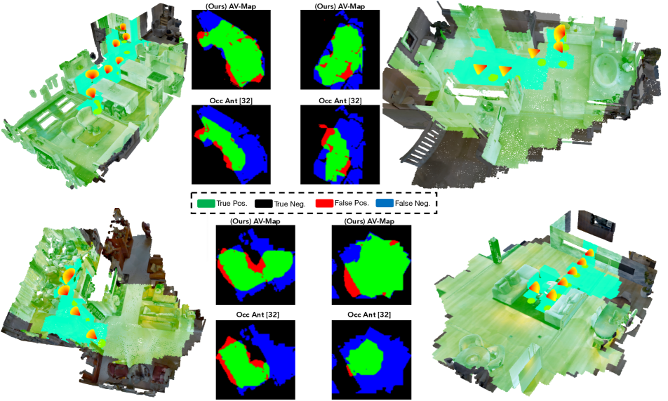
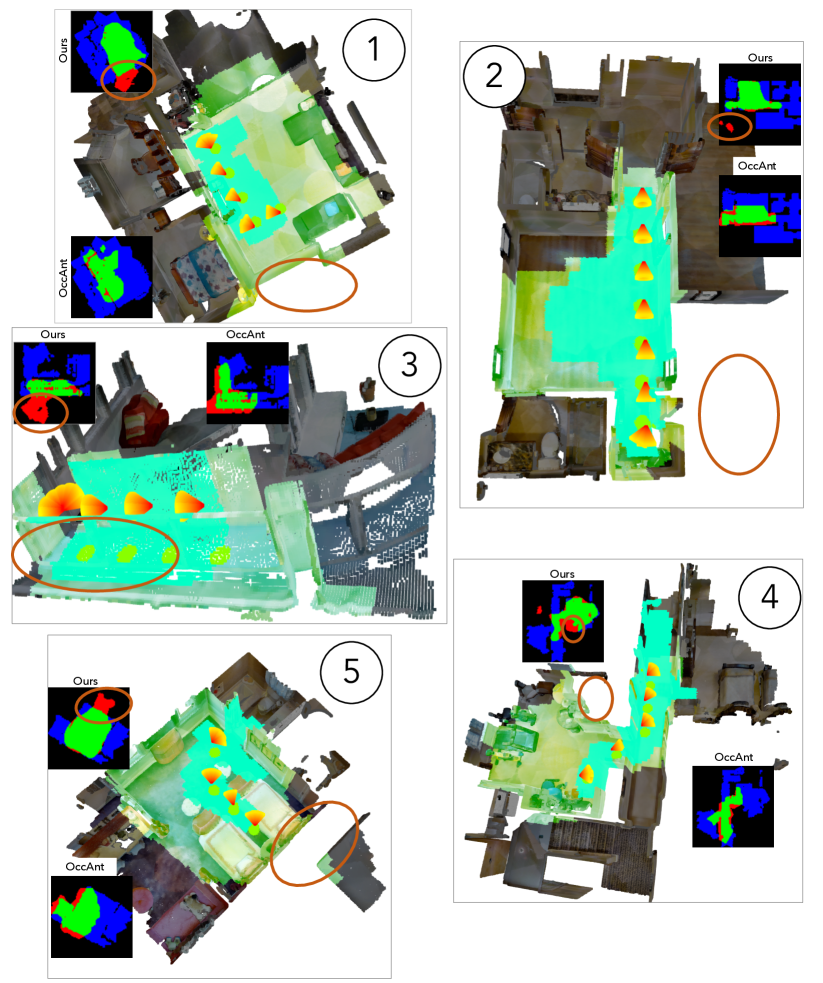
Our proposed AV-Map model using the device-generated audio outperforms all the baselines on all three metrics. Furthermore, our full AV model outperforms the audio-only and RGB-only variants by good margins. This shows our model successfully performs joint inference by leveraging important cues from both modalities. Our model with RGB-only is itself stronger than the baselines from existing literature [33, 13], showing the strength of our proposed framework even without the advantage of audio. Fig. 3 shows example map predictions compared to [33], the best existing method. They highlight how audio allows “seeing" both behind the camera as well as inferring freespace behind walls in large multi-room homes.
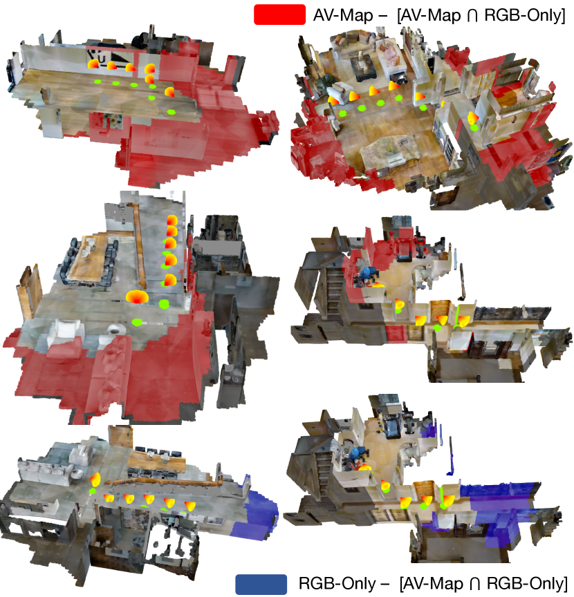
Fig. 4 compares examples from AV-Map and its RGB-only variant.
| AP | Acc. | Edge AP | ||
|---|---|---|---|---|
| RGB-only | 69.05 | 64.20 | 52.93 | |
| Dev. Gen. | Audio-only | 70.44 | 63.06 | 52.85 |
| Audio-Visual | 73.67 | 66.51 | 55.21 | |
| Env. Telephone | Audio-only | 68.60 | 63.53 | 53.27 |
| Audio-Visual | 72.30 | 66.69 | 54.16 | |
| Env. Nearby | Audio-only | 66.27 | 61.49 | 51.86 |
| Audio-Visual | 72.86 | 66.16 | 54.32 | |
| Env. All Room | Audio-only | 65.42 | 61.41 | 51.98 |
| Audio-Visual | 71.38 | 65.46 | 54.79 |
Comparison of Audio Settings: Table 2 compares our AV-Map model in the three audio settings described in Sec 3.4. Our model performs slightly better when operated in the device-generated audio setting. This is expected since the frequency sweep audio allows us to capture all the frequencies in the audible range, unlike the naturally occurring sounds in the environment-generated settings. Furthermore, the relative location of the source is known in the device-generated setting (since it is always at the camera).
In every setting, AV-Map outperforms the RGB-only and Audio-only ablations. Despite the challenges in Env. All Room (multiple simultaneous sounds from different source locations), we observe minimal decline in our interior map performance.
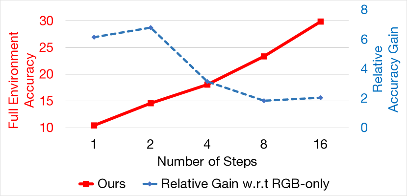
Effect of Trajectory Length: Figure 5 shows our full-house accuracy gains as a function of trajectory length.333Absolute numbers are lower than in Tab. 1 because the scored area here is the entire house’s area, vs. the maximum output map area in Tab. 1. Our model outperforms the RGB-only ablation consistently across varying trajectory lengths. Importantly, our gains are largest when the video is shorter, when less area is visible. This again confirms the power of audio to “see" beyond the images. As the length increases, the visible fraction of the environment becomes larger, diminishing the impact of audio signals (dotted blue line).
| RGB-Only | Audio-only | AV-Map | |
| Mean AP | 9.42 | 13.30 | 14.12 |
4.2 Floorplan Room Classification
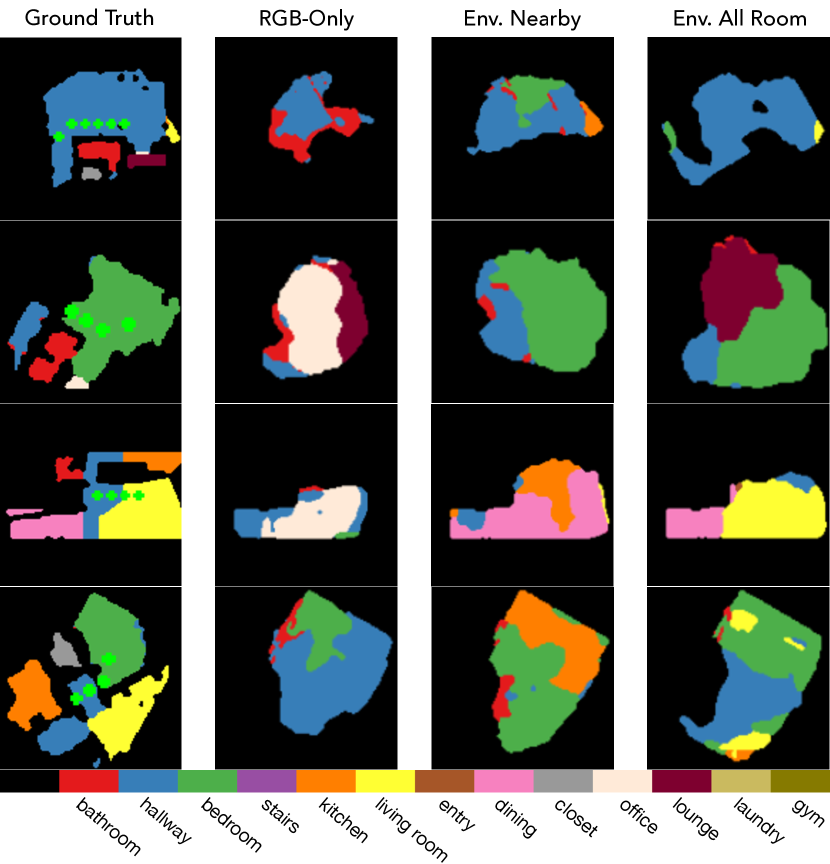
Finally, we evaluate the semantic room label maps. We evaluate with environment-generated audio, which provides natural object-room cues. Figure 6 compares the mean of the pixel-wise room classification average precision for our proposed model in the Env. Gen. All Room setting and its ablations.444Note that the baselines from Table 1 are not applicable here because they produce only geometric interior maps. Results are averaged over all trajectory lengths. Audio can identify rooms in the neighborhood of the trajectory, and we see best results when both modalities are used together. The room map examples show AV-Map provides better room classification compared to our RGB-only variant, and does best with many natural semantic sounds—encouraging for deployment in a busy household. Our model can identify the correct room type and its approximate location, though without actually entering a room, its exact footprint naturally remains ambiguous.
5 Conclusion and Future Work
We proposed a new research direction: audio-visual floorplan reconstruction from short video sequences. We developed a multi-modal model to estimate the floorplan around and far beyond the camera trajectory. Our AV-Map model successfully infers the structure and semantics of areas that are not visible, outperforming the state-of-the-art in extrapolated visual maps. In future work we plan to consider extensions to multi-level floorplans and connect our mapping idea to a robotic agent actively controlling the camera.
6 Acknowledgements
We would like to thank Unnat Jain, Changan Chen, and Santhosh Kumar Ramakrishnan for help with generating the audio simulations and providing help with code for this work. We would also like to thank Ruohan Gao for providing feedback on the text.
References
- [1] T. Abhayapala and D. Ward. Theory and design of higher order sound field microphones using spherical microphone array. In ICASSP, 2002.
- [2] Marcus A. Brubaker, Andreas Geiger, and Raquel Urtasun. Lost! leveraging the crowd for probabilistic visual self-localization. In CVPR, 2013.
- [3] Angel Chang, Angela Dai, Thomas Funkhouser, Maciej Halber, Matthias Niessner, Manolis Savva, Shuran Song, Andy Zeng, and Yinda Zhang. Matterport3d: Learning from rgb-d data in indoor environments. arXiv preprint arXiv:1709.06158. Matterport3D license available at http://kaldir.vc.in.tum.de/matterport/MP_TOS.pdf., 2017.
- [4] Devendra Singh Chaplot, Dhiraj Gandhi, Saurabh Gupta, Abhinav Gupta, and Ruslan Salakhutdinov. Learning to explore using active neural slam. arXiv preprint arXiv:2004.05155, 2020.
- [5] Changan Chen, Unnat Jain, Carl Schissler, Sebastia Vicenc Amengual Gari, Ziad Al-Halah, Vamsi Krishna Ithapu, Philip Robinson, and Kristen Grauman. Audio-visual embodied navigation. arXiv preprint arXiv:1912.11474, 2019.
- [6] Changan Chen, Unnat Jain, Carl Schissler, Sebastia Vicenc Amengual Gari, Ziad Al-Halah, Vamsi Krishna Ithapu, Philip Robinson, and Kristen Grauman. Soundspaces: Audio-visual navigation in 3d environments. In ECCV, 2020.
- [7] Changan Chen, Sagnik Majumder, Ziad Al-Halah, Ruohan Gao, Santhosh Kumar Ramakrishnan, and Kristen Grauman. Learning to set waypoints for audio-visual navigation. In arXiv, 2020.
- [8] Jiacheng Chen, Chen Liu, Jiaye Wu, and Yasutaka Furukawa. Floor-sp: Inverse cad for floorplans by sequential room-wise shortest path. In Proceedings of the IEEE International Conference on Computer Vision, pages 2661–2670, 2019.
- [9] Tao Chen, Saurabh Gupta, and Abhinav Gupta. Learning exploration policies for navigation. In 7th International Conference on Learning Representations, ICLR 2019, 2019.
- [10] Jesper Haahr Christensen, Sascha Hornauer, and X Yu Stella. Batvision: Learning to see 3d spatial layout with two ears. In 2020 IEEE International Conference on Robotics and Automation (ICRA), pages 1581–1587. IEEE, 2020.
- [11] Marco Crocco, Samuele Martelli, Andrea Trucco, Andrea Zunino, and Vittorio Murino. Audio tracking in noisy environments by acoustic map and spectral signature. EEE Trans Cybern, 2018.
- [12] Victoria Dean, Shubham Tulsiani, and Abhinav Gupta. See, hear, explore: Curiosity via audio-visual association. Advances in Neural Information Processing Systems, 33, 2020.
- [13] Ivan Dokmanić, Reza Parhizkar, Andreas Walther, Yue M Lu, and Martin Vetterli. Acoustic echoes reveal room shape. Proceedings of the National Academy of Sciences, 110(30):12186–12191, 2013.
- [14] Itamar Eliakim, Zahi Cohen, Gabor Kosa, and Yossi Yovel. A fully autonomous terrestrial bat-like acoustic robot. PLoS computational biology, 14(9):e1006406, 2018.
- [15] Chuang Gan, Yiwei Zhang, Jiajun Wu, Boqing Gong, and Joshua B Tenenbaum. Look, listen, and act: Towards audio-visual embodied navigation. In 2020 IEEE International Conference on Robotics and Automation (ICRA), pages 9701–9707. IEEE, 2020.
- [16] Chuang Gan, Hang Zhao, Peihao Chen, David Cox, and Antonio Torralba. Self-supervised moving vehicle tracking with stereo sound. In ICCV, 2019.
- [17] R. Gao, C. Chen, Z. Al-Halah, C. Schissler, and K. Grauman. VisualEchoes: Spatial image representation learning through echolocation. In ECCV, 2020.
- [18] Jort Gemmeke, Daniel Ellis, Dylan Freedman, Aren Jansen, Wade Lawrence, Channing Moore, Manoj Plakal, and Marvin Ritter. Audio set: An ontology and human-labeled dataset for audio events. In ICASSP, 2017.
- [19] Dimitrios Giannoulis, Emmanouil Benetos, Dan Stowell, Mathias Rossignol, Mathieu Lagrange, and Mark D. Plumbley. Detection and classification of acoustic scenes and events: An ieee aasp challenge. In IEEE Workshop on Applications of Signal Processing to Audio and Acoustics, 2013.
- [20] Saurabh Gupta, David Fouhey, Sergey Levine, and Jitendra Malik. Unifying map and landmark based representations for visual navigation. arXiv preprint arXiv:1712.08125, 2017.
- [21] R. Hartley and A. Zisserman. Multiple View Geometry in Computer Vision. 2004.
- [22] D. Jayaraman and K. Grauman. Learning to look around: Intelligently exploring unseen environments for unknown tasks. In CVPR, 2018.
- [23] H. Jeong and Y. Lam. Source implementation to eliminate low-frequency artifacts in finite difference time domain room acoustic simulation. Journal of the Acoustical Society of America, 2012.
- [24] Abhishek Kadian, Joanne Truong, Aaron Gokaslan, Alexander Clegg, Erik Wijmans, Stefan Lee, Manolis Savva, Sonia Chernova, and Dhruv Batra. Are we making real progress in simulated environments? measuring the sim2real gap in embodied visual navigation. arXiv preprint arXiv:1912.06321, 2019.
- [25] Hansung Kim, Luca Remaggi, Philip JB Jackson, Filippo Maria Fazi, and Adrian Hilton. 3d room geometry reconstruction using audio-visual sensors. In 2017 International Conference on 3D Vision (3DV), pages 621–629. IEEE, 2017.
- [26] Chen-Yu Lee, Vijay Badrinarayanan, Tomasz Malisiewicz, and Andrew Rabinovich. Roomnet: End-to-end room layout estimation. In ICCV, 2017.
- [27] David B Lindell, Gordon Wetzstein, and Vladlen Koltun. Acoustic non-line-of-sight imaging. In Proceedings of the IEEE Conference on Computer Vision and Pattern Recognition, pages 6780–6789, 2019.
- [28] Chen Liu, Jiaye Wu, and Yasutaka Furukawa. Floornet: A unified framework for floorplan reconstruction from 3d scans. In Proceedings of the European Conference on Computer Vision (ECCV), pages 201–217, 2018.
- [29] Medhini Narasimhan, Erik Wijmans, Xinlei Chen, Trevor Darrell, Dhruv Batra, Devi Parikh, and Amanpreet Singh. Seeing the un-scene: Learning amodal semantic maps for room navigation. arXiv preprint arXiv:2007.09841, 2020.
- [30] Brian Okorn, Xuehan Xiong, Burcu Akinci, and Daniel Huber. Toward automated modeling of floor plans. In 3DPVT, 2009.
- [31] Andrew Owens, Phillip Isola, Josh McDermott, Antonio Torralba, Edward H Adelson, and William T Freeman. Visually indicated sounds. In Proceedings of the IEEE conference on computer vision and pattern recognition, pages 2405–2413, 2016.
- [32] B. Rafaely. Analysis and design of higher order sound field microphones using spherical microphone array. IEEE Trans. on Speech and Audio Processing, 2005.
- [33] Santhosh K Ramakrishnan, Ziad Al-Halah, and Kristen Grauman. Occupancy anticipation for efficient exploration and navigation. arXiv preprint arXiv:2008.09285, 2020.
- [34] J. Santos, D. Portugal, and R. Rocha. An evaluation of 2d slam techniques available in robot operating system. In IEEE International Symposium on Safety, Security, and Rescue Robotics (SSRR), 2013.
- [35] Nikolay Savinov, Alexey Dosovitskiy, and Vladlen Koltun. Semi-parametric topological memory for navigation. arXiv preprint arXiv:1803.00653, 2018.
- [36] Manolis Savva, Abhishek Kadian, Oleksandr Maksymets, Yili Zhao, Erik Wijmans, Bhavana Jain, Julian Straub, Jia Liu, Vladlen Koltun, Jitendra Malik, et al. Habitat: A platform for embodied ai research. In Proceedings of the IEEE International Conference on Computer Vision, pages 9339–9347, 2019.
- [37] S. Se, D. Lowe, and J. Little. Mobile robot localization and mapping with uncertainty using scale-invariant visual landmarks. IJRR, 2002.
- [38] Jascha Sohl-Dickstein, Santani Teng, Benjamin M Gaub, Chris C Rodgers, Crystal Li, Michael R DeWeese, and Nicol S Harper. A device for human ultrasonic echolocation. IEEE Transactions on Biomedical Engineering, 62(6):1526–1534, 2015.
- [39] Shuran Song, Andy Zeng, Angel X. Chang, Manolis Savva, Silvio Savarese, and Thomas Funkhouser. Im2pano3d: Extrapolating 360 structure and semantics beyond the field of view. In CVPR, 2018.
- [40] Julian Straub, Thomas Whelan, Lingni Ma, Yufan Chen, Erik Wijmans, Simon Green, Jakob J Engel, Raul Mur-Artal, Carl Ren, Shobhit Verma, et al. The replica dataset: A digital replica of indoor spaces. arXiv preprint arXiv:1906.05797, 2019.
- [41] Wei Sui, Lingfeng Wang, Bin Fan, Hongfei Xiao, Huaiyu Wu, and Chunhong Pan. Layer-wise floorplan extraction for automatic urban building reconstruction. IEEE Transactions on Visualization and Computer Graphics, 2016.
- [42] Cheng Sun, Chi-Wei Hsiao, Min Sun, and Hwann-Tzong Chen. Horizonnet: Learning room layout with 1d representation and pano stretch data augmentation. In CVPR, 2019.
- [43] Ashish Vaswani, Noam Shazeer, Niki Parmar, Jakob Uszkoreit, Llion Jones, Aidan N Gomez, Łukasz Kaiser, and Illia Polosukhin. Attention is all you need. In Advances in neural information processing systems, pages 5998–6008, 2017.
- [44] Antonio Pico Villalpando, Guido Schillaci, Verena V Hafner, and Bruno Lara Guzmán. Ego-noise predictions for echolocation in wheeled robots. In Artificial Life Conference Proceedings, pages 567–573. MIT Press, 2019.
- [45] S. Yang, F. Wang, C. Peng, P. Wonka, M. Sun, and H. Chu. Dula-net: A dual-projection network for estimating room layouts from a single rgb panorama. In CVPR, 2019.
- [46] Mao Ye, Yu Zhang, Ruigang Yang, and Dinesh Manocha. 3d reconstruction in the presence of glasses by acoustic and stereo fusion. In Proceedings of the IEEE Conference on Computer Vision and Pattern Recognition, pages 4885–4893, 2015.
- [47] Zhoutong Zhang, Jiajun Wu, Qiujia Li, Zhengjia Huang, James Traer, Josh H McDermott, Joshua B Tenenbaum, and William T Freeman. Generative modeling of audible shapes for object perception. In Proceedings of the IEEE International Conference on Computer Vision, pages 1251–1260, 2017.
- [48] Chuhang Zou, Alex Colburn, Qi Shan, and Derek Hoiem. Layoutnet: Reconstructing the 3d room layout from a single rgb image. In CVPR, 2018.
- [49] Chuhang Zou, Jheng-Wei Su, Chi-Han Peng, Alex Colburn, Qi Shan, Peter Wonka, Hung-Kuo Chu, and Derek Hoiem. 3d manhattan room layout reconstruction from a single 360 image. arXiv preprint arXiv:1910.04099, 2019.
(Supplementary Material) Audio-Visual Floorplan Reconstruction
Appendix A Additional Interior Map Visualizations
Figure 7 presents additional AV-Map interior map prediction visualizations, like Fig 3 in the main text. We see again how our model sees beyond the visible portions (cyan) to more fully map the space. We also highlight our failure modes; see the mis-classified locations (circled) on the predicted maps. We observe that the errors often arise in challenging locations that are not visually covered, where the model relies on the audio signal (see Figure 7 sample 1,4,5). Some errors arise from noise in the scan of the environment (see Figure 7 sample 3 - missing point cloud) since the rendered RGB frames are noisy.
Appendix B Room Map Visualizations and Confusion Analysis
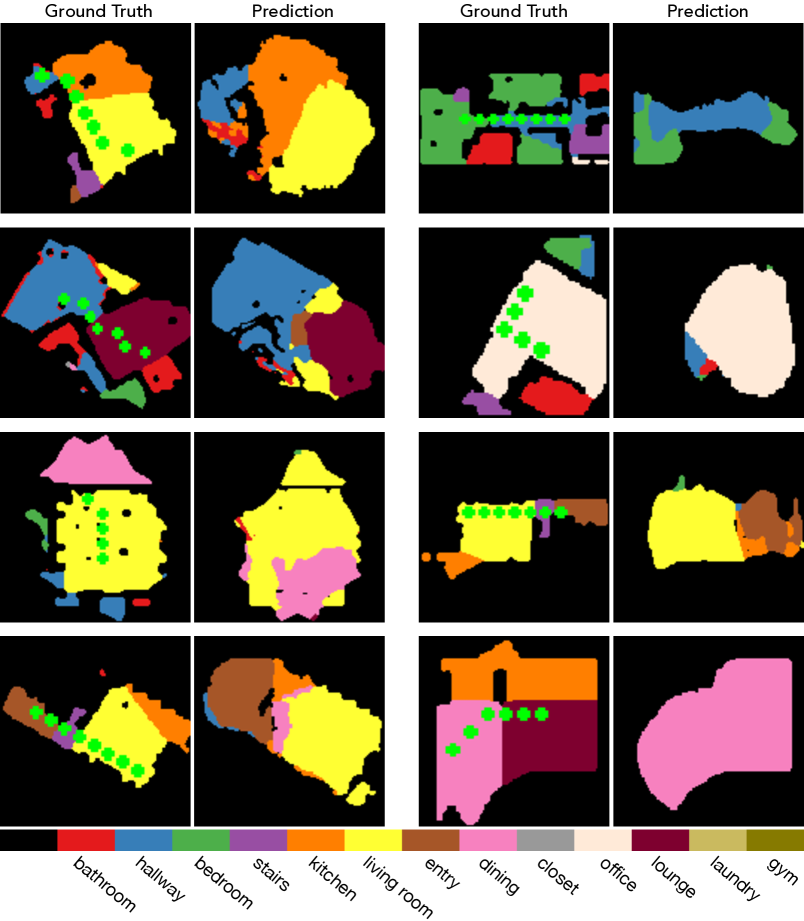
In Figure 8, we present additional visualizations for the estimated room maps. The room maps were generated by the AV-Map model operating in the environment generated all-room audio setting. Green dots on the ground truth indicate the camera positions. From these visualizations, we observe that the model can successfully identify the approximate locations of several rooms. Some sources of errors are errors in interior estimation (see Column 1, Row 4 and Column 2, Row 3) and errors in localization of the rooms (see Column 1, Row 3).
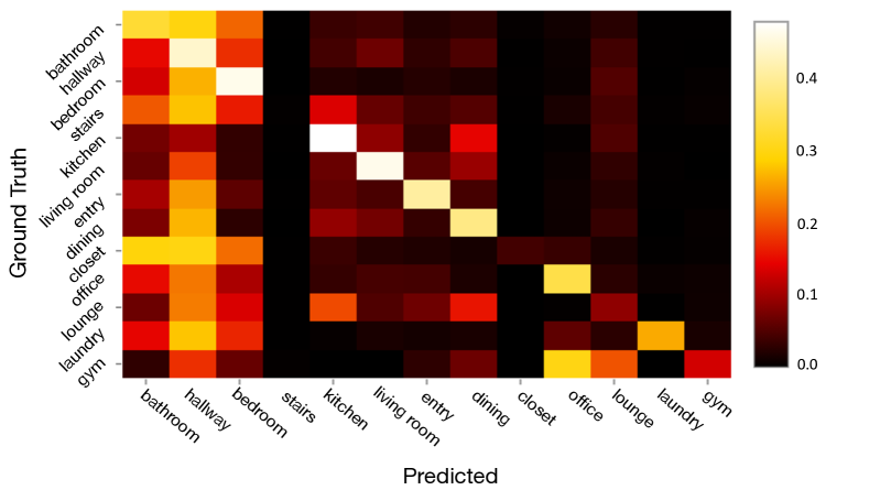
In Figure 9, we present a confusion matrix for the pixel-wise room label predictions. We observe that there is a bias towards predicting the “bathroom”, “hallway” and “bedroom” classes which are the three most frequent room labels. The two least frequent classes (“stairs” and “closet”) are almost never predicted. This indicates that our model could benefit from training on a larger, more diverse and more balanced dataset. We also find that the rooms that are usually in close proximity have slightly higher confusion rates - for example, bedroom vs bathroom, and dining room vs kitchen. This suggests that our model struggles to accurately localize the boundaries of rooms (as also indicated in the main text).
Appendix C Importance of Sequence Modeling
At each time step of a video, the audio clip is generated by convolving a downloaded audio clip with an impulse response . Therefore, the audio clip can be expressed as:
| (8) | |||
| OR | |||
| (9) |
where is the Fourier transform. The impulse response encodes the acoustic characteristics of the environment for the given source location and receiver location pair at the time step . These acoustic characteristics of the environment strongly depend on the geometric and material properties of the environments. Therefore, in order to infer the geometric properties of the environment, a model should ideally be able to either disentangle the impulse response from the audio clip or infer a function of the impulse response from . This is not possible from the audio clip at a single time step unless the audio clip is known apriori. However, listening to audio clips from multiple time steps , , can allow us to model relative changes in impulse responses as:
| (10) |
These relative changes can also provide information about the geometric properties of the environment. For example, walking past a door of a room containing a sound source will see a large change in impulse response clearly indicating the presence of an opening. Note here that the inferred relative change in impulse response does not rely on the original audio clip anymore. This is also a favorable feature since downloaded audio clips are not 100% anechoic. So in practice the audio clips encode the acoustic characteristics of the recording environment i.e. where is the anechoic audio and is the impulse response of the recording setup. While we do not explicitly enforce the AV-Map model to infer these relative changes, training with multiple audio clips forces the model to learn to disentangle the effect of the impulse response.
The proposed AV-Map model allows training and testing with video sequences of arbitrary length. During training, the primary bottleneck for using very long sequences is the memory footprint and speed of computation. Training with is equivalent to making independent predictions at each time step and pooling them to obtain the final interior map estimate. For each time step, such a model would not be able to make inferences using visual features in other time steps (for example, the fact that the camera entered a door in the first step provides additional context at the second time step). Furthermore, as explained above, making independent predictions does not allow us to model relative changes in the impulse responses. We observed that sequences of length provide the benefits of modeling sequences while maintaining a manageable training duration. As promised in the main paper, in Table 3, we show results with and compare to the setting to demonstrate the impact of sequence modeling.
| AP | Acc. | Edge AP | |
|---|---|---|---|
| Single Step () | 68.91 | 62.46 | 54.05 |
| Sequence () | 73.61 | 66.51 | 55.21 |
Appendix D Predicting interior area
In the main text, we presented a quantitative analysis of the AV-Map model trained to estimate interior maps for an area of 40 around the camera at each time step (by setting hyper-parameters ). As promised in Section 4.1 of the main paper, here in Table 4, we present similar quantitative results555Note that the positive and negative pixels are balanced by reweighting as discussed in Section 4.1 for a model trained to predict a 164 area around the camera at each step. We observe similar results demonstrating the improved performance of the AV-Map model compared to the RGB-only model.
| Number of Steps | 1 | 2 | 4 | 8 | 16 |
|---|---|---|---|---|---|
| RGB only | 72.05 | 72.45 | 72.60 | 75.05 | 76.00 |
| Dev. Gen. | 73.59 | 75.00 | 75.10 | 78.75 | 80.71 |
| Env. Nearby | 73.01 | 73.36 | 74.08 | 78.03 | 79.76 |
| Env. All Room | 72.33 | 73.55 | 74.76 | 77.67 | 80.29 |
Appendix E Additional Dataset Details
Environments
We use the Matterport3D[3] dataset to generate video sequences (see Sec 3.4 of the main text). We use the splits provided by the SoundSpaces [6] dataset for training, validation, and testing. We include the environments in the splits here for reference:
Train environments: [’17DRP5sb8fy’, ’1LXtFkjw3qL’, ’1pXnuDYAj8r’, ’29hnd4uzFmX’, ’5LpN3gDmAk7’, ’5q7pvUzZiYa’, ’759xd9YjKW5’, ’7y3sRwLe3Va’, ’82sE5b5pLXE’, ’8WUmhLawc2A’, ’aayBHfsNo7d’, ’ac26ZMwG7aT’, ’B6ByNegPMKs’, ’b8cTxDM8gDG’, ’cV4RVeZvu5T’, ’D7N2EKCX4Sj’, ’e9zR4mvMWw7’, ’EDJbREhghzL’, ’GdvgFV5R1Z5’, ’gTV8FGcVJC9’, ’HxpKQynjfin’, ’i5noydFURQK’, ’JeFG25nYj2p’, ’JF19kD82Mey’, ’jh4fc5c5qoQ’, ’kEZ7cmS4wCh’, ’mJXqzFtmKg4’, ’p5wJjkQkbXX’, ’Pm6F8kyY3z2’, ’pRbA3pwrgk9’, ’PuKPg4mmafe’, ’PX4nDJXEHrG’, ’qoiz87JEwZ2’, ’rPc6DW4iMge’, ’s8pcmisQ38h’, ’S9hNv5qa7GM’, ’sKLMLpTHeUy’, ’SN83YJsR3w2’, ’sT4fr6TAbpF’, ’ULsKaCPVFJR’, ’uNb9QFRL6hY’, ’Uxmj2M2itWa’, ’V2XKFyX4ASd’, ’VFuaQ6m2Qom’, ’VVfe2KiqLaN’, ’Vvot9Ly1tCj’, ’vyrNrziPKCB’, ’VzqfbhrpDEA’, ’XcA2TqTSSAj’, ’D7G3Y4RVNrH’, ’E9uDoFAP3SH’, ’JmbYfDe2QKZ’, ’r1Q1Z4BcV1o’, ’r47D5H71a5s’, ’ur6pFq6Qu1A’, ’VLzqgDo317F’, ’YmJkqBEsHnH’, ’ZMojNkEp431’]
Val environments: [’2azQ1b91cZZ’, ’8194nk5LbLH’, ’EU6Fwq7SyZv’, ’oLBMNvg9in8’, ’QUCTc6BB5sX’, ’TbHJrupSAjP’, ’X7HyMhZNoso’, ’pLe4wQe7qrG’, ’x8F5xyUWy9e’, ’Z6MFQCViBuw’, ’zsNo4HB9uLZ’]
Test environments: [’5ZKStnWn8Zo’, ’ARNzJeq3xxb’, ’fzynW3qQPVF’, ’jtcxE69GiFV’, ’pa4otMbVnkk’, ’q9vSo1VnCiC’, ’rqfALeAoiTq’, ’UwV83HsGsw3’, ’wc2JMjhGNzB’, ’WYY7iVyf5p8’, ’YFuZgdQ5vWj’, ’yqstnuAEVhm’, ’gxdoqLR6rwA’, ’gYvKGZ5eRqb’, ’Vt2qJdWjCF2’]
Room types and associated sounds
For generating room maps, we choose the 13 most frequent room types. For each room type, we download sounds from www.freesound.org generated by objects (or people) that are unique to the room type. Here we present the list of rooms, their associated sounds, and the number of train/val/test sounds for each:
-
•
bathroom: brushing (3/2/2), flush(4/1/1)
-
•
hallway: <no sound>
-
•
bedroom: alarm clock (5/3/3)
-
•
stairs: footsteps (5/3/3)
-
•
kitchen: blender (3/1/1), cabinet (1/1/1), dishwasher (3/2/2)
-
•
living room: telephone (5/3/3)
-
•
entryway/foyer/lobby: knock (5/2/2)
-
•
dining room: knife (4/1/1) , spoon(4/2/2)
-
•
closet: closet door (2/2/2)
-
•
office: keyboard (5/3/3)
-
•
lounge: no sound
-
•
laundryroom/mudroom: washing machine (5/3/3)
-
•
workout/gym/exercise: person panting (5/3/3)
Appendix F Implementation and Training Details
F.1 Hyperparameters
The AV-Map model is trained with a batchsize of 32 videos using 4 GPUs. Each sample in the batch is generated by randomly sampling a camera trajectory as described in the main text. We use the SGD optimizer with a starting learning rate of 0.1, momentum 0.9 and weight decay 0.00001. After 30000 SGD updates, we drop the learning rate to 0.01 and train for an additional 20000 SGD steps.
F.2 Positional Encoding
The positional encoding map added in the feature alignment stage (see Sec 3.2) is a 64-channel 2D map representing the position of each pixel with a 64 dimensional vector. For position (i,j) in the feature map, the positional encoding is computed as:
| (11) |
F.3 Feature Alignment
Here we present a pseudo-code to illustrate the feature alignment described in Section 3.2.