Provably Training Overparameterized Neural Network Classifiers with Non-convex Constraints

Abstract

Training a classifier under non-convex constraints has gotten increasing attention in the machine learning community thanks to its wide range of applications such as algorithmic fairness and class-imbalanced classification. However, several recent works addressing non-convex constraints have only focused on simple models such as logistic regression or support vector machines. Neural networks, one of the most popular models for classification nowadays, are precluded and lack theoretical guarantees. In this work, we show that overparameterized neural networks could achieve a near-optimal and near-feasible solution of non-convex constrained optimization problems via the project stochastic gradient descent. Our key ingredient is the no-regret analysis of online learning for neural networks in the overparameterization regime, which may be of independent interest in online learning applications.

1 Introduction

In many real-world machine learning problems, practitioners are not only interested in the performance of their models but also need to meet societal and legal goals, while taking advantage of side information, prior knowledge, and unlabeled data. For example, in the classification task, fairness metrics with respect to certain sensitive characteristics, such as gender or ethnicity [23], are measured to correct biased training data and improve the accuracy [13]; F-measure, G-mean, and H-mean [28, 50, 45] are used with class-imbalanced data to prevent trivial solutions; the classifier churn [56] is computed to improve prediction stability. All metrics mentioned above involve non-convex functions of the prediction output, and one could cast the learning task of training a classification model satisfying the above metrics as a constrained optimization problem. Several challenges arise due to non-convex and data-dependent constraints that were partially addressed in the context of linear models [56, 31, 47, 59]. Neural networks, which are widely used for classification and enjoy tremendous empirical success in practice, are not covered by the theoretical guarantees developed in these papers.

In this paper, we consider the problem of training a neural network classifier under non-convex constraints through the lens of the neural tangent kernel. Since neural network models are non-convex, we face the problem of non-convexity arising from both the constraints and the model. To establish the convergence rate in this challenging setting, we follow the minimax optimization strategy studied in [59]. Specifically, we formulate the optimization problem with non-differentiable and non-convex constraints as an unconstrained minimax optimization problem using the Lagrangian and then iteratively update model parameters, Lagrange multipliers, and auxiliary variables with convex surrogate functions for non-convex constraints. Although the optimization framework in [59] is rather general, it cannot be directly applied to our problem due to the non-convexity of neural networks.

Our contribution is threefold. First, we prove the first convergence result for overparameterized neural network classifiers with non-convex constraints. In particular, our result states that a neural network classifier can achieve a near-optimal and near-feasible solution as long as the width of the neural network is large enough. Second, a no-regret guarantee is provided for online learning problems with neural networks in the overparameterization regime. The no-regret analysis may be of independent interest for online learning with neural network models and related applications. Our no-regret analysis follows by extending the conventional no-regret analysis to the online mirror descent with stochastic biased gradients. Such biased gradient analysis is studied in machine learning applications, including model-agnostic meta-learning and federated learning [30, 68, 19]. Finally, unlike the prior work [59], our approach does not require any best response function or oracle for optimization. We emphasize that an oracle that provides a near-optimal solution for non-convex problems may not exist in practice, and the projected stochastic gradient descent is a scalable and practical algorithm for large-scale datasets and optimization problems with neural networks. As a result, our approach leads to a simple and computationally efficient procedure.

1.1 Related Work

Our work is related to the literature on non-convex constrained optimization, algorithmic fairness, and neural tangent kernels. We summarize the literature most related to the current work and do not attempt to provide an extensive survey.

Non-convex constrained optimization. Non-convex minimization problems with non-convex constraints have been recently studied due to their popularity in the machine learning community [16, 14]. [57, 58] developed stochastic algorithms based on sequential quadratic programming that incorporate a stochastic line search and converge globally to a first-order stationary point of the optimization program. [18] and [1] used a Lagrangian-based approach with access to an optimization oracle and found a distribution over solutions rather than a pure equilibrium. [27] interpreted the resulting Lagrangian as a non-zero-sum two-player game. Their theoretical result guarantees the feasibility regarding the original constraints rather than the proxy constraints. Another approach to address non-convex constraints is to study weak notions of convexity [29]. In particular, [55] studied constrained optimization in which both the objective and the constraints are weakly convex. They solved a sequence of strongly convex subproblems and established the computational complexity to find a nearly stationary point.

Algorithmic fairness. Algorithmic fairness is an important application of our non-convex constrained optimization framework. Many papers have studied different approaches to fulfill algorithmic fairness in machine learning [40, 46, 12, 17]. In particular, [69] included the correlation between the decision boundary and sensitive attributes as a constraint on the learned classifier. [31] and [63] designed constrained optimization problems that enforce the learned classifiers to have similar errors on the positive class independently of subgroups.

Neural tangent kernel. There is a considerable body of literature that analyzes deep supervised learning with overparameterized neural networks [71, 61, 53, 33]. [5] and [8] studied two-layer neural networks in the overparametrization regime, where neural networks can be approximated by linear models with the neural tangent kernel [43, 51, 3]. This phenomenon of local linearization provides a powerful tool to circumvent the obstacle of the non-convexity of neural networks and establish convergence properties. [22] and [6] showed that neural networks approximate a subset of the reproducing kernel Hilbert space induced by some kernels. See [36] for a recent review. Compared to previous work, we extend the approximation results of neural networks to the setting of online learning. Based on our new technique, we show that neural networks can be trained under non-convex constraints and the corresponding convergence rate.

1.2 Notations

We use bold capital letters ($\mathbf{A},\mathbf{B},\dots$) to denote matrices, bold lowercase letters ($\mathbf{a},\mathbf{b},\dots$) to denote column vectors, and lowercase or uppercase letters ($a,b,\dots A,B,\dots$) for constants. With slight abuse of notation, we use bold lowercase ($\mathbf{f},\mathbf{g},\dots$) and lowercase ($f,g,h,\dots$) letters for a mapping or random element whose codomain is $\mathbb{R}^{n}$ and $\mathbb{R}$, respectively, with an exception $\mathcal{L}$ which is used for Lagrangian function. We write $\mathbf{a}=(a_{1},\dots,a_{m})^{\top}$.

For a continuous function $f:\operatorname{dom}f\subset\mathbb{R}^{n}\rightarrow\mathbb{R}$, where $\operatorname{dom}f$ is the domain of $f$, $\nabla f(\mathbf{x})$ denotes the gradient of $f$ evaluated at $\mathbf{x}\in\operatorname{dom}f$. Given a vector $\mathbf{x}=(x_{1},\dots,x_{n})^{\top}\in\mathbb{R}^{n}$, $\nabla_{x_{i}}f(\mathbf{x})$ denotes the partial derivative of $f$ corresponding to the variable $x_{i}$. We use $\|\cdot\|_{2}$ and $\|\cdot\|_{\infty}$ to denote the $\ell_{2}$-norm and the infinity norm, respectively. For a general norm $\|\cdot\|$, we use $\|\cdot\|_{\ast}$ to denote its dual norm.

Given a set $\mathcal{E}=\{e_{1},\dots,e_{k}\}$ and a probability vector $\mathbf{p}\in\mathbb{R}^{k}$ such that $\sum_{i=1}^{k}p_{i}=1$, $\text{categorical}(\mathcal{E},\mathbf{p})$ is the categorical distribution on $\{1,\dots,k\}$ such that $\mathbb{P}(e_{i})=p_{i}$, and $\text{Uniform}(\mathcal{E})$ is the discrete uniform distribution on $\mathcal{E}$ with size $k$ such that $\text{Uniform}(\mathcal{E})=\text{categorical}(\mathcal{E},(1/k,\dots,1/k))$. We use $[n]$ to denote the set $\{1,2,\dots,n\}$.

For a subset ${\mathcal{S}}\subset\mathbb{R}^{n}$, the operator $\Pi_{S}$ denotes the projection to $S$ with respect to the Euclidean norm $\|\cdot\|_{2}$. Given two sequences $a_{k},b_{k}$, we write $a_{k}=O(b_{k})$ if there exists a positive real number $c$ such that $a_{k}\leq cb_{k}$ for all large enough $k$.

1.3 Organization

The rest of the paper is organized as follows. Section 2 sets up our problem and a minimax optimization framework as well as the details of the optimization procedure to solve our problem. Section 3 discusses our main convergence results in this paper, and Section 4 presents numerical experiments on real-world datasets. Conclusion and the future work is provided in Section 5.

2 Problem Setup

We start by introducing a general formulation of a non-convex constrained optimization problem. Subsequently, we present few concrete examples that can be studied in the general framework. Finally, we discuss the neural network predictor as well as a minimax optimization framework to solve the non-convex constrained optimization problem.

2.1 Optimization Formulation

Let $\mathbf{x}$ denote a feature vector in an instance space $\mathcal{X}\subset\mathbb{R}^{d}$ and let $z$ denote a label in a label space $\mathcal{Z}=\{-1,1\}$. The goal is to train a model $y(\bm{\theta};\mathbf{x})$ by finding a parameter $\bm{\theta}$ in a parameter space $\Theta$ that minimizes the following constrained optimization problem:

$$\begin{split}\min_{\bm{\theta}\in\Theta}&\ \mathbb{E}_{(\mathbf{x},z)\sim\mathcal{D}_{0}}[h_{0}(y(\bm{\theta};\mathbf{x}),z)]\\ \text{s.t.}&\ g_{j}\left(\mathbb{E}_{(\mathbf{x},z)\sim\mathcal{D}_{1}}[h_{1}(y(\bm{\theta};\mathbf{x}),z)],\dots,\mathbb{E}_{(\mathbf{x},z)\sim\mathcal{D}_{K}}[h_{K}(y(\bm{\theta};\mathbf{x}),z)]\right)\leq 0,\ j\in[J],\end{split}$$ (1)

where $\{\mathcal{D}_{k}\}_{k=0}^{K}$ are some distributions on $\mathcal{X}\times\mathcal{Z}$, $d$ is the dimension of the instance space, $h_{0}$ is a convex loss function that evaluates the distance between the model $y(\bm{\theta};\mathbf{x})$ and the label $z$ (for example, hinge loss). The formulation in (1) is inspired by a wide range of applications including algorithmic fairness [40, 31], class-imbalance classification [45, 49], KL-divergence based metrics used in quantification tasks [39, 35]. We will discuss concrete examples of the optimization problem (1) in detail in the next section.

There are three major difficulties in solving the optimization problem in (1): (i) non-convexity of $h_{k}$, (ii) data-dependent constraints which may be computationally challenging to check, (iii) properly sampling distributions $\mathcal{D}_{k}$. The third problem is beyond the scope of this paper and we present only computational issues related to formulation (1). We tackle the first two challenges by converting (1) into a minimax optimization, and, in the corresponding Lagrangian, we replace $h_{k}$ by its convex upper bound, which will be discussed in detail at the end of this section. A similar idea is used when solving different optimization problems, such as the generalized eigenvalue problem [21] and the canonical correlation analysis [20] that also involve data-dependent constraints. However, our ultimate interest is in neural networks, which require different tools from those in the existing literature.

2.2 Concrete Examples

We present practical examples that motivate our optimization problem in (1). Note that our theory is capable but not limited to solving those examples in this section, as our non-convex constrained optimization is general enough for many other real-world applications.

Classical Classification. The first example is the classification task aiming to minimize the following accuracy (0-1 loss) without any constraints

$$\min_{\bm{\theta}}\mathbb{E}_{(\mathbf{x},z)\sim\mathcal{D}_{p}}\operatorname*{1{\hskip-2.5pt}\hbox{$\rm{I}$}}\{z=\mathop{\mathrm{sign}}(y(\bm{\theta};\mathbf{x}))\},$$ (2)

where $\mathcal{D}_{p}$ is defined as the population distribution of a data set, $\operatorname*{1{\hskip-2.5pt}\hbox{$\rm{I}$}}$ is the indicator function, and $\mathop{\mathrm{sign}}$ is the sign function. Since minimizing the 0-1 loss problem is an NP-hard problem [37], the conventional solution is to replace the 0-1 loss by a hinge loss, which is a convex upper bound for the 0-1 loss [41]. The same idea can be applied to constraint functions $h_{k}$ when considering the optimization problem in (1) in its Lagrangian form.

Algorithmic Fairness. In many classification problems, such as the approval of a loan or admission to a college, the outcome $z=1$ is often treated as the advantaged outcome. Let $\mathcal{A}\subset\mathcal{X}$ be a protected subgroup, and let $D_{\mathcal{A}}$ and $D_{\mathcal{A}^{c}}$ denote the conditional distributions of $(\mathbf{x},z)$ given $\mathbf{x}\in\mathcal{A},z=1$ and $\mathbf{x}\in\mathcal{A}^{c},z=1$, respectively. With this notation, the probabilities that protected and unprotected subgroups get advantaged outcome are

$$\mathbb{E}_{(\mathbf{x},z)\sim\mathcal{D}_{\mathcal{A}}}\operatorname*{1{\hskip-2.5pt}\hbox{$\rm{I}$}}\{z=\mathop{\mathrm{sign}}(y(\bm{\theta};\mathbf{x}))\},\ \ \ \mathbb{E}_{(\mathbf{x},z)\sim\mathcal{D}_{\mathcal{A}^{c}}}\operatorname*{1{\hskip-2.5pt}\hbox{$\rm{I}$}}\{z=\mathop{\mathrm{sign}}(y(\bm{\theta};\mathbf{x}))\}.$$ (3)

In the literature on algorithmic fairness, the predictor $y(\bm{\theta};\mathbf{x})$ is said to satisfy equal opportunity [40] if

$$\mathbb{E}_{(\mathbf{x},z)\sim\mathcal{D}_{\mathcal{A}}}\operatorname*{1{\hskip-2.5pt}\hbox{$\rm{I}$}}\{z=\mathop{\mathrm{sign}}(y(\bm{\theta};\mathbf{x}))\}=\mathbb{E}_{(\mathbf{x},z)\sim\mathcal{D}_{\mathcal{A}^{c}}}\operatorname*{1{\hskip-2.5pt}\hbox{$\rm{I}$}}\{z=\mathop{\mathrm{sign}}(y(\bm{\theta};\mathbf{x}))\},$$ (4)

which means that the recall on different subgroups should be aligned and the probability that the protected and unprotected subgroups get advantaged outcome should be equal. Note that removing sensitive features usually cannot result in equal opportunity, as there may exist other features that are highly correlated with the sensitive features.

Training a classifier that satisfies the fairness requirement stated in (4) can be cast as

$$\begin{split}\min_{\bm{\theta}\in\Theta}&\ \mathbb{E}_{(\mathbf{x},z)\sim\mathcal{D}_{p}}\operatorname*{1{\hskip-2.5pt}\hbox{$\rm{I}$}}\{z=\mathop{\mathrm{sign}}(y(\bm{\theta};\mathbf{x}))\},\\ \text{s.t.}&\ \mathbb{E}_{(\mathbf{x},z)\sim\mathcal{D}_{\mathcal{A}}}\operatorname*{1{\hskip-2.5pt}\hbox{$\rm{I}$}}\{z=\mathop{\mathrm{sign}}(y(\bm{\theta};\mathbf{x}))\}=\mathbb{E}_{(\mathbf{x},z)\sim\mathcal{D}_{\mathcal{A}^{c}}}\operatorname*{1{\hskip-2.5pt}\hbox{$\rm{I}$}}\{z=\mathop{\mathrm{sign}}(y(\bm{\theta};\mathbf{x}))\},\end{split}$$ (5)

which can be rewritten as

$$\begin{split}\min_{\bm{\theta}\in\Theta}&\ \mathbb{E}_{(\mathbf{x},z)\sim\mathcal{D}_{p}}\operatorname*{1{\hskip-2.5pt}\hbox{$\rm{I}$}}\{z=\mathop{\mathrm{sign}}(y(\bm{\theta};\mathbf{x}))\},\\ \text{s.t.}&\ \mathbb{E}_{(\mathbf{x},z)\sim\mathcal{D}_{\mathcal{A}}}\operatorname*{1{\hskip-2.5pt}\hbox{$\rm{I}$}}\{z=\mathop{\mathrm{sign}}(y(\bm{\theta};\mathbf{x}))\}+\mathbb{E}_{(\mathbf{x},z)\sim\mathcal{D}_{\mathcal{A}^{c}}}[-\operatorname*{1{\hskip-2.5pt}\hbox{$\rm{I}$}}\{z=\mathop{\mathrm{sign}}(y(\bm{\theta};\mathbf{x}))\}]\leq 0,\\ &\ \mathbb{E}_{(\mathbf{x},z)\sim\mathcal{D}_{\mathcal{A}}}[-\operatorname*{1{\hskip-2.5pt}\hbox{$\rm{I}$}}\{z=\mathop{\mathrm{sign}}(y(\bm{\theta};\mathbf{x}))\}]+\mathbb{E}_{(\mathbf{x},z)\sim\mathcal{D}_{\mathcal{A}^{c}}}\operatorname*{1{\hskip-2.5pt}\hbox{$\rm{I}$}}\{z=\mathop{\mathrm{sign}}(y(\bm{\theta};\mathbf{x}))\}\leq 0.\end{split}$$ (6)

Therefore, training a classifier that meets the fairness requirement by minimizing (5) is covered by the formulation in (1).

Imbalance data. When the data have class imbalance (for example, when $\mathbb{P}(z=1)$ is small), finding a classifier that optimizes only the classification accuracy can lead to a trivial model $y(\bm{\theta};\mathbf{x})$ that outputs only the majority class, for example, $y(\bm{\theta};\mathbf{x})=-1$ for all $\mathbf{x}$. Several evaluation metrics that involve precision and recall, such as the F-score, $2/(\text{recall}^{-1}+\text{precision}^{-1})$, are remedies for naive accuracy in the class-imbalanced classification task. Furthermore, let $\operatorname{TPR}=\mathbb{E}_{(\mathbf{x},z)\sim\mathcal{D}_{+}}\operatorname*{1{\hskip-2.5pt}\hbox{$\rm{I}$}}\{z=\mathop{\mathrm{sign}}(y(\bm{\theta};\mathbf{x}))\}$ and $\operatorname{TNR}=\mathbb{E}_{(\mathbf{x},z)\sim\mathcal{D}_{-}}\operatorname*{1{\hskip-2.5pt}\hbox{$\rm{I}$}}\{z=\mathop{\mathrm{sign}}(y(\bm{\theta};\mathbf{x}))\}$ be the true positive and true negative rates corresponding to the predictor $y(\bm{\theta};\mathbf{x})$, where $\mathcal{D}_{+}$ and $\mathcal{D}_{-}$ are the conditional distribution of $(\mathbf{x},z)$ given $z=1$ and $z=0$, respectively. Then, choosing $g_{1}(\bm{\xi})=1-\sqrt{\xi_{1}\xi_{2}}$ and $g_{1}(\bm{\xi})=1-2/(1/\xi_{1}+1/\xi_{2})$, we recover $\operatorname{G-mean}=1-\sqrt{\text{TPR}\times\text{TNR}}$ [49] and $\operatorname{H-mean}=1-2/(1/\text{TPR}+1/\text{TNR})$ [45], which shows that class-imbalanced classification problems are included in the formulation (9).

2.3 Prediction Model: Two-layer Neural Network

We focus on a two-layer neural network model

$$y(\bm{\theta};\mathbf{x})=\frac{1}{\sqrt{m}}\sum_{i=1}^{m}b_{i}\sigma(\mathbf{a}_{i}^{\top}\mathbf{x}),$$ (7)

where $m$ is the width of the neural network, $b_{i}\in\{-1,1\}$ are the output weights, $\sigma(u)=\max(0,u)$ is the rectified linear unit (ReLU) activation function, and $\bm{\theta}=(\mathbf{a}_{1}^{\top},\dots,\mathbf{a}_{m}^{\top})^{\top}\in\Theta\subset\mathbb{R}^{md}$ is the input weight. Figure 1 provides a visualization of a two-layer neural network. As $m\rightarrow\infty$, the class of functions defined in (7) approximates a subset of the reproducing kernel Hilbert space induced by the kernel

$$K(\mathbf{x}_{1},\mathbf{x}_{2})=\mathbb{E}_{\mathbf{a}\sim\mathcal{N}({\bf 0},\mathbf{I}_{d}/d)}[\operatorname*{1{\hskip-2.5pt}\hbox{$\rm{I}$}}\{\mathbf{a}^{\top}\mathbf{x}_{1}>0\}\operatorname*{1{\hskip-2.5pt}\hbox{$\rm{I}$}}\{\mathbf{a}^{\top}\mathbf{x}_{2}>0\}\mathbf{x}_{1}^{\top}\mathbf{x}_{2}].$$

This function class is sufficiently rich, if the width $m$ and the radius $D$ are sufficiently large [8].

Figure 1: The visualization of the two-layer neural network.

The neural network is initialized by the following scheme

$$b_{i}\sim\text{Uniform}(\{-1,1\}),\quad\mathbf{a}_{i}^{0}\sim\mathcal{N}({\bf 0},\mathbf{I}_{d}/d),$$ (8)

where $\mathcal{N}({\bf 0},\mathbf{I}_{d}/d)$ denotes the multivariate normal distribution with mean ${\bf 0}$ and covariance matrix $\mathbf{I}_{d}/d$ and $\mathbf{I}_{d}$ is the identity matrix of size $d$. During training, $\bm{\theta}$ is restricted to the search space $\bm{\Theta}=\{\bm{\theta}:\|\bm{\theta}-\bm{\theta}^{0}\|_{2}\leq D\}$, where $D$ is a predefined constant. That is, $\bm{\theta}$ is restricted to an $\ell_{2}$ ball centered at initialization $\bm{\theta}^{0}=((\mathbf{a}_{1}^{0})^{\top},\dots,(\mathbf{a}_{m}^{0})^{\top})^{\top}$ and $b_{i}$ is fixed for simplicity and omitted from $\bm{\theta}$. Such a setup is commonly used in the literature [4, 5, 7, 64]. Note that $\mathbf{a}_{i}^{0}\sim\mathcal{N}({\bf 0},\mathbf{I}_{d}/d)$, which is different from the literature that usually sets $\mathbf{a}_{i}^{0}\sim\mathcal{N}({\bf 0},\mathbf{I}_{d}/m)$. In our setting, $\|\bm{\theta}^{0}\|$ does not converge to a fixed number in probability as $m\rightarrow\infty$. Instead, we prove that $y(\bm{\theta};\mathbf{x})$ lies in a compact domain with high probability. This observation is crucial for the regret analysis of online learning. See Proposition 3.

2.4 A Minimax Optimization Framework and its Optimization Procedure

We introduce a minimax optimization framework to solve the optimization problem (1). In particular, the Lagrangian multiplier method is applied to recast the constrained optimization problem into an unconstrained minimax problem. We introduce auxiliary variables and rewrite (1) as

$$\begin{split}\min_{\bm{\theta}\in\Theta,\bm{\xi}\in\Xi}&\ r_{0}(\bm{\theta})\ \ \text{s.t.}\ \mathbf{g}\left(\bm{\xi}\right)\leq{\bf 0},\ \mathbf{r}(\bm{\theta})\leq\bm{\xi},\end{split}$$ (9)

where $\mathbf{g}=(g_{1},\dots,g_{J})^{\top}$, $r_{k}(\bm{\theta})=\mathbb{E}_{(\mathbf{x},z)\sim\mathcal{D}_{k}}[h_{k}(y(\bm{\theta};\mathbf{x});z)]$, $\mathbf{r}=(r_{1},\dots,r_{K})^{\top}$, and $\Xi$ is the space of $\bm{\xi}$, which is defined in (16) below. Assumption 2, given in the following section, further imposes conditions that ensure that (9) and (1) are equivalent. The Lagrangian corresponding to (9) is

$$\mathcal{L}(\bm{\theta},\bm{\xi},\bm{\lambda})=r_{0}(\bm{\theta})+\sum_{j=1}^{J}\lambda_{j}g_{j}(\bm{\xi})-\sum_{k=1}^{K}\lambda_{J+k}\xi_{k}+\sum_{k=1}^{K}\lambda_{J+k}r_{k}(\bm{\theta}),$$ (10)

where $\bm{\lambda}=(\lambda_{1},\dots,\lambda_{J},\lambda_{J+1},\dots,\lambda_{K+J})^{\top}\geq{\bf 0}$ is the vector of Lagrange multipliers corresponding to the $K$ auxiliary variables and $J$ constraints. Since the functions $h_{k}$ are non-convex, we assume that there exist convex surrogate functions $\widetilde{h}_{k}$ which upper bound $h_{k}$, that is, $\widetilde{h}_{k}$ are convex and $h_{k}(y,z)\leq\widetilde{h}_{k}(y,z)$ for all $(y,z)\in\mathbb{R}\times\mathcal{Z}$. Such convex surrogate functions generally exist. For example, the hinge loss is the convex surrogate function for the 1-0 loss that satisfies this requirement. We assume that $\widetilde{h}_{k}$ are differentiable, but it is not difficult to extend our argument to non-differentiable surrogate functions by using subgradient method. Finally, we also define $\widetilde{r}_{k}(\bm{\theta})=\mathbb{E}_{(\mathbf{x},z)\sim\mathcal{D}_{k}}[\widetilde{h}_{k}(y(\bm{\theta};\mathbf{x});z)]$.

A key observation is that the surrogate functions $\widetilde{h}_{k}$ are needed only to optimize the Lagrangian with respect to $\bm{\theta}$. This observation plays an important role in obtaining guarantees regarding the true feasible sets. Letting

$$\begin{split}\mathcal{L}_{1}(\bm{\xi},\bm{\lambda})&=\sum_{j=1}^{J}\lambda_{j}g_{j}(\bm{\xi})-\sum_{k=1}^{K}\lambda_{J+k}\xi_{k},\ \ \mathcal{L}_{2}(\bm{\theta},\bm{\lambda})=r_{0}(\bm{\theta})+\sum_{k=1}^{K}\lambda_{J+k}r_{k}(\bm{\theta}),\\ \widetilde{\mathcal{L}}_{2}(\bm{\theta},\bm{\lambda})&=r_{0}(\bm{\theta})+\sum_{k=1}^{K}\lambda_{J+k}\widetilde{r}_{k}(\bm{\theta}),\ \ \widetilde{\mathcal{L}}=\mathcal{L}_{1}+\widetilde{\mathcal{L}}_{2},\end{split}$$ (11)

we can solve (9) by alternating the following steps: minimizing $\widetilde{\mathcal{L}}_{2}$ with respect to $\bm{\theta}$, minimizing $\mathcal{L}_{1}$ with respect to $\bm{\xi}$, and maximizing $\mathcal{L}$ with respect to $\bm{\lambda}$. In particular, the projected stochastic gradient descent is used in each of these steps to update the parameters $\bm{\theta}$, $\bm{\xi}$, and $\bm{\lambda}$. Given samples $\mathbf{x}_{t+1},z_{t+1}\sim\mathcal{D}_{0}$ and $\mathbf{x}_{t+1,k},z_{t+1,k}\sim\mathcal{D}_{k}$, the unbiased estimators of gradients $\nabla_{\bm{\theta}}\widetilde{\mathcal{L}}_{2}(\bm{\theta},\bm{\lambda})$ and $\nabla_{\bm{\lambda}}\mathcal{L}(\bm{\theta},\bm{\xi},\bm{\lambda})$ are

$$\begin{split}\widehat{\nabla}_{\bm{\theta}}\widetilde{\mathcal{L}}_{2}(\bm{\theta},\bm{\lambda})&=\nabla_{\bm{\theta}}h_{0}(y(\bm{\theta};\mathbf{x}_{t+1}),z_{t+1})+\sum_{k=1}^{K}\lambda_{J+k}\nabla_{\bm{\theta}}\widetilde{h}_{k}(y(\bm{\theta};\mathbf{x}_{t+1,k}),z_{t+1,k}),\\ \widehat{\nabla}_{\bm{\lambda}}\mathcal{L}(\bm{\theta},\bm{\xi},\bm{\lambda})&=\begin{pmatrix}g_{1}(\bm{\xi})\\ \vdots\\ g_{J}(\bm{\xi})\\ h_{1}(y(\bm{\theta};\mathbf{x}_{t+1,1}),z_{t+1,1}^{\prime})-\xi_{1}\\ \vdots\\ h_{K}(y(\bm{\theta};\mathbf{x}_{t+1,K}),z_{t+1,K})-\xi_{K}\end{pmatrix},\end{split}$$ (12)

and the gradient $\nabla_{\bm{\xi}}\mathcal{L}_{1}(\bm{\xi},\bm{\lambda})$ can be obtained as

$$\nabla_{\bm{\xi}}\mathcal{L}_{1}(\bm{\xi},\bm{\lambda})=\left(\sum_{j=1}^{J}\lambda_{j}\nabla_{\xi_{1}}g_{j}(\bm{\xi})-\lambda_{J+1},\dots,\sum_{j=1}^{J}\lambda_{j}\nabla_{\xi_{K}}g_{j}(\bm{\xi})-\lambda_{J+K}\right)^{\top}.$$ (13)

We summarize the projected stochastic gradient descent in Algorithm 1.

Input: $\bm{\theta}^{0}\in\Theta,\bm{\xi}^{0}\in\Xi,\bm{\lambda}^{0}\in\Lambda,\eta_{\theta},\eta_{\xi},\eta_{\lambda}$

for $t=1$ to $T$ do

       Sample $\mathbf{x}_{t+1},z_{t+1}\sim\mathcal{D}_{0}$ and $\mathbf{x}_{t+1,k},z_{t+1,k}\ \sim\mathcal{D}_{k}$;

       Compute $\widehat{\nabla}_{\bm{\theta}}\widetilde{\mathcal{L}}_{2}(\bm{\theta}^{t},\bm{\lambda}^{t}),\nabla_{\bm{\xi}}\mathcal{L}_{1}(\bm{\xi}^{t},\bm{\lambda}^{t}),\widehat{\nabla}_{\bm{\lambda}}\mathcal{L}(\bm{\theta}^{t},\bm{\xi}^{t},\bm{\lambda}^{t})$ via (12) and (13);

       $\bm{\theta}^{t+1}=\Pi_{\Theta}(\bm{\theta}^{t}-\eta_{\theta}\widehat{\nabla}_{\bm{\theta}}\widetilde{\mathcal{L}}_{2}(\bm{\theta}^{t},\bm{\lambda}^{t}))$ ;

       $\bm{\xi}^{t+1}=\Pi_{\Xi}(\bm{\xi}^{t}-\eta_{\xi}\nabla_{\bm{\xi}}\mathcal{L}_{1}(\bm{\xi}^{t},\bm{\lambda}^{t}))$ ;

       $\bm{\lambda}^{t+1}=\Pi_{\Lambda}(\bm{\lambda}^{t}+\eta_{\lambda}\widehat{\nabla}_{\bm{\lambda}}\mathcal{L}(\bm{\theta}^{t},\bm{\xi}^{t},\bm{\lambda}^{t}))$ ;

      

end for

Algorithm 1 Stochastic projected gradient descent

We end this section by providing an informal statement on the convergence of the stochastic projected gradient descent used to train the classifier parameterized by a neural network (7).

Theorem 1 (Informal main theorem).

Suppose that regularity conditions hold and that parameters are properly tuned. Then, with high probability, we have

$$\frac{1}{T}\sum_{t=1}^{T}r_{0}(\bm{\theta}^{t})-\min_{\theta\in\Theta\cap\widetilde{\mathcal{F}}}r_{0}(\bm{\theta})\leq O\left(\frac{\kappa D^{3/2}}{\sqrt{T}}+\frac{\kappa D^{5/2}}{m^{1/4}}\right),$$ (14)

and, for $j=1,\dots,J$,

$$g_{j}\left(\frac{1}{T}\sum_{t=1}^{T}\mathbf{r}(\bm{\theta}^{t})\right)\leq O\left(\frac{D^{3/2}}{\sqrt{T}}+\frac{D^{2}}{\kappa}+\frac{D^{5/2}}{m^{1/4}}\right),$$ (15)

where $\widetilde{\mathcal{F}}=\{\bm{\theta}:\max_{j}g_{j}(\widetilde{\mathbf{r}}(\theta))\leq 0\}$.

Theorem 1 is the first result on the convergence of neural networks for non-convex constrained optimization problems. Since Theorem 1 provides results in terms of $\frac{1}{T}\sum r_{k}(\bm{\theta}^{t})$, using the convexity of $r_{0}$ and $g_{j}$, it can be shown that a stochastic classifier, defined in Algorithm 2, achieves a near-optimal and near feasible solution for the constrained optimization problem in (1) after training the model $y(\bm{\theta};\mathbf{x})$ for $T$ iterations. In Algorithm 2, we select a random parameter after training the model for $T$ iterations, which is common in the literature on non-convex optimization [44] and online learning [66]. From Theorem 1 it follows that when the width $m$ increases, the approximation error converges to zero. This result is due to the fact that an infinitely wide neural network is similar to a linear model, a phenomenon called local linearization that plays an important role in our analysis. We provide ingredients for the theoretical analysis and a detailed statement of the main results in the following section.

Input: A data point $\mathbf{x}$, a predictor $y(\bm{\theta};\mathbf{x})$, $\{\bm{\theta}^{t}\}_{t=1}^{T}$ and $\mathbf{p}$ such that $\sum_{t}p_{t}=1$

Output: $y(\bm{\theta}^{i};x)$ where $i\sim\text{categorical}(T,\mathbf{p})$

Algorithm 2 Stochastic classifier

3 Main Results

We provide several intermediate steps that are needed to prove Theorem 1. In particular, we discuss how to find an equilibrium by an online learning procedure with non-convex losses and local linearization of neural networks. For simplicity, we only consider the binary classification task and two-layer neural networks. However, with additional efforts, our ideas can be extended to multi-class classification and deep neural networks.

3.1 Achieving a Near-optimal and Near-feasible Solution from Coarse-correlated Equilibrium

We present a the convergence result for the minimax optimization framework. We need the following assumption on the objective function and constraints.

Assumption 2.

Let

$$\begin{split}\mathcal{Y}&=\{y:|y|\leq 2D\},\ \ \ \Theta=\{\bm{\theta}:\|\bm{\theta}-\bm{\theta}^{0}\|\leq D\},\\ \Xi&=\left\{\bm{\xi}:|\bm{\xi}|\leq\sup_{y\in\mathcal{Y},z\in\mathcal{Z}}|\widetilde{h}_{k}(y,z)|\right\},\ \ \ \Lambda=\left\{\bm{\lambda}\geq{\bf 0}:\|\bm{\lambda}\|_{\infty}\leq\kappa\right\},\end{split}$$ (16)

define the domain of every variable, where $\kappa$ and $D$ are predefined constants. The objective function and constraints in (9) satisfy the following restrictions:

1. $h_{0}$ is differentiable and convex, and $\operatorname{dom}h_{k}=\mathbb{R}$;

2. There exists a constant $C$ such that for all $0\leq k\leq K$

   $$\sup_{y\in\mathcal{Y},z\in\mathcal{Z}}|h_{k}(y,z)|\leq C;$$ (17)

3. There exist functions $\widetilde{h}_{k}$ such that each $\widetilde{h}_{k}$ is differentiable and convex, $h_{k}(y,z)\leq\widetilde{h}_{k}(y,z)$ for all $(y,z)\in\mathbb{R}\times\mathcal{Z}$ and $k=1,\dots,K$, and

   $$\sup_{y\in\mathcal{Y},z\in\mathcal{Z}}|\widetilde{h}_{k}(y,z)|\leq C;$$ (18)

4. The function $g_{j}$ is strictly jointly convex, monotonically increasing in each argument, $\sup_{\bm{\xi}\in\Xi}|g_{j}(\bm{\xi})|\leq C$, and $L$-Lipschitz with respect to the infinity norm, $\|\cdot\|_{\infty}$, for all $j=1,\dots,J$.

We have several comments on Assumption 2:

(a) The boundedness assumptions for the domain of variables are crucial regular conditions to derive the local linearization in Section 3.3 and the no-regret bound for online learning in Section 3.2. As a result, despite the fact that the behavior of local linearization around the initialization is not specific to overparameterized neural networks and may not fully explain their successes [22], the boundedness assumption is natural in our setting. In other words, although the weights $\bm{\theta}$ are indeed a measure of generalization [60] and regularization on weights can improve the generalization [48, 9, 65], restricting $\bm{\theta}$ on $\Theta=\{\bm{\theta}:\|\bm{\theta}-\bm{\theta}^{0}\|_{2}\leq D\}$ and using projected gradient descent may not be practical for training neural networks. However, since projections into some compact domain are necessary for both online learning and local linearization, projected stochastic gradient descent is a natural choice for optimization in our setting.

(b) The differentiability assumptions are made for simplicity. It is not hard to extend our results to the case without differentiability via a subgradient method.

(c) Note that we do not assume $h_{k}$ is convex for $k=1,\dots,K$. Therefore, we need the assumption of existence of convex surrogate functions $\widetilde{h}_{k}$, which is also a conventional solution for overcoming non-convexity in practice [41]. The upper boundedness is important for the guarantee of feasibility. In particular, the upper boundedness condition yields that $r_{k}(\bm{\theta})\leq\widetilde{r}_{k}(\bm{\theta})$, so the fact that $\bm{\lambda}\geq{\bf 0}$ implies

$$\mathcal{L}_{2}(\bm{\theta},\bm{\lambda})\leq\widetilde{\mathcal{L}}_{2}(\bm{\theta},\bm{\lambda})\Rightarrow\mathcal{L}(\bm{\theta},\bm{\lambda})\leq\widetilde{\mathcal{L}}(\bm{\theta},\bm{\lambda}).$$ (19)

(d) The bound $\sup_{y\in\mathcal{Y},z\in\mathcal{Z}}|\widetilde{h}_{k}(y,z)|\leq C$ always holds due to compactness of $\mathcal{Y}$ and $\mathcal{Z}$ and continuity of $\widetilde{h}_{k}$.

(e) The last assumption ensures that (9) and (1) are equivalent.

(f) In spite of its popularity, the F-score is not included in our framework since we cannot find a function $g$ satisfying the last part of Assumption 2.

Before discussing our theoretical results, we take algorithmic fairness in Section 2.2 as an example to illustrate Assumption 2.

Example 1.

Consider the classification problem with fairness constraints:

$$\begin{split}\min_{\bm{\theta}\in\Theta}&\ \mathbb{E}_{(\mathbf{x},z)\sim\mathcal{D}_{p}}h_{0}(y(\bm{\theta};\mathbf{x}),z),\\ \text{s.t.}&\ \mathbb{E}_{(\mathbf{x},z)\sim\mathcal{D}_{\mathcal{A}}}\operatorname*{1{\hskip-2.5pt}\hbox{$\rm{I}$}}\{z=\mathop{\mathrm{sign}}(y(\bm{\theta};\mathbf{x}))\}+\mathbb{E}_{(\mathbf{x},z)\sim\mathcal{D}_{\mathcal{A}^{c}}}[-\operatorname*{1{\hskip-2.5pt}\hbox{$\rm{I}$}}\{z=\mathop{\mathrm{sign}}(y(\bm{\theta};\mathbf{x}))\}]\leq 0,\\ &\ \mathbb{E}_{(\mathbf{x},z)\sim\mathcal{D}_{\mathcal{A}}}[-\operatorname*{1{\hskip-2.5pt}\hbox{$\rm{I}$}}\{z=\mathop{\mathrm{sign}}(y(\bm{\theta};\mathbf{x}))\}]+\mathbb{E}_{(\mathbf{x},z)\sim\mathcal{D}_{\mathcal{A}^{c}}}\operatorname*{1{\hskip-2.5pt}\hbox{$\rm{I}$}}\{z=\mathop{\mathrm{sign}}(y(\bm{\theta};\mathbf{x}))\}\leq 0.\end{split}$$ (20)

In this classification problem, we have

$$\begin{split}h_{1}(y(\bm{\theta};\mathbf{x}),z)=\operatorname*{1{\hskip-2.5pt}\hbox{$\rm{I}$}}\{z=\mathop{\mathrm{sign}}(y(\bm{\theta};\mathbf{x}))\},&\ \ h_{2}(y(\bm{\theta};\mathbf{x}),z)=-\operatorname*{1{\hskip-2.5pt}\hbox{$\rm{I}$}}\{z=\mathop{\mathrm{sign}}(y(\bm{\theta};\mathbf{x}))\}]\\ h_{3}(y(\bm{\theta};\mathbf{x}),z)=\operatorname*{1{\hskip-2.5pt}\hbox{$\rm{I}$}}\{z=\mathop{\mathrm{sign}}(y(\bm{\theta};\mathbf{x}))\},&\ \ h_{4}(y(\bm{\theta};\mathbf{x}),z)=-\operatorname*{1{\hskip-2.5pt}\hbox{$\rm{I}$}}\{z=\mathop{\mathrm{sign}}(y(\bm{\theta};\mathbf{x}))\}]\\ g_{1}(\xi_{1},\xi_{2},\xi_{3},\xi_{4})=\xi_{1}+\xi_{4},&\ \ g_{2}(\xi_{1},\xi_{2},\xi_{3},\xi_{4})=\xi_{2}+\xi_{3},\end{split}$$ (21)

and the function $h_{0}$ is the hinge loss $h_{0}(y(\bm{\theta};\mathbf{x}),z)=\max(0,1-zy(\bm{\theta};\mathbf{x}))$. Since the hinge loss is the convex upper bound of the zero-one loss, we can set $\widetilde{h}_{1}$ and $\widetilde{h}_{3}$ as the hinge loss. Similarly, we can let $\widetilde{h}_{2}(y(\bm{\theta};\mathbf{x}),z)=\max(-1,zy(\bm{\theta};\mathbf{x}))=\widetilde{h}_{4}(y(\bm{\theta};\mathbf{x}),z)$, which shows the existence of functions $\widetilde{h}_{k}$. Note that $\operatorname*{1{\hskip-2.5pt}\hbox{$\rm{I}$}}$ and $\mathop{\mathrm{sign}}$ are non-convex functions such that $0\leq\operatorname*{1{\hskip-2.5pt}\hbox{$\rm{I}$}}\{z=\mathop{\mathrm{sign}}(y(\bm{\theta};\mathbf{x}))\}\leq 1$ for all $(\mathbf{x},z)\in\mathcal{X}\times\mathcal{Z}$. As a result, it is clear that other conditions in Assumption 2 are satisfied since $\mathcal{Y}$ is compact and $g_{j}$ are linear. It is true that $\widetilde{h}$ is not differentiable, but we can smooth the $\max$ function and make $\widetilde{h}$ differentiable.

We are ready to present our theoretical results for the minimax optimization framework. Under Assumption 2, Proposition 4 establishes the relationship between an approximate coarse-correlated equilibrium of minimax optimization and the solution of (9). The proof is based on the ideas in [59]. However, we improve these ideas by using an approximate equilibrium for $\bm{\xi}$ instead of the best response or an oracle for optimization. As a result, we can use projected stochastic gradient descent to alternatively update $\bm{\xi},\bm{\theta},\bm{\lambda}$ on large-scale data sets. Our technique is more suitable for neural network models since stochastic gradient descent is the workhorse used to train neural networks. This improvement is based on the following observation.

Proposition 3.

Suppose that $\|\mathbf{x}\|\leq 1$ for all $\mathbf{x}\in\mathcal{X}$. Then $|y(\bm{\theta};\mathbf{x})|<2D$ with probability $1-B/D$ for some constant $B$.

Proof.

See Appendix B.1 for a proof. ∎

Proposition 3 can be easily extended to an arbitrary distribution of $\{b_{i}\}$ using the martingale theory [24] as long as $\{b_{i}\}$ are independent. We present our main result in Proposition 4.

Proposition 4.

Suppose Assumption 2 and conditions of Proposition 3 hold. If $(\bm{\theta}^{t},\bm{\xi}^{t},\bm{\lambda}^{t})\in\Theta\times\Xi\times\Lambda$ comprises an approximate coarse-correlated equilibrium, that is, if it satisfies

$$\frac{1}{T}\sum_{t=1}^{T}\mathcal{L}_{1}(\bm{\xi}^{t},\bm{\lambda}^{t}) \leq\min_{\bm{\xi}\in\Xi}\frac{1}{T}\sum_{t=1}^{T}\mathcal{L}_{1}(\bm{\xi},\bm{\lambda}^{t})+\epsilon_{\xi},$$ (22a)

$$\frac{1}{T}\sum_{t=1}^{T}\widetilde{\mathcal{L}}_{2}(\bm{\theta}^{t},\bm{\lambda}^{t}) \leq\min_{\bm{\theta}\in\Theta}\frac{1}{T}\sum_{t=1}^{T}\widetilde{\mathcal{L}}_{2}(\bm{\theta},\bm{\lambda}^{t})+\epsilon_{\theta},$$ (22b)

$$\frac{1}{T}\sum_{t=1}^{T}{\mathcal{L}}(\bm{\theta}^{t},\bm{\xi}^{t},\bm{\lambda}^{t}) \geq\max_{\bm{\lambda}\in\Lambda}\frac{1}{T}\sum_{t=1}^{T}{\mathcal{L}}(\bm{\theta}^{t},\bm{\xi}^{t},\bm{\lambda})-\epsilon_{\lambda},$$ (22c)

where $\varepsilon_{\xi},\varepsilon_{\theta},\varepsilon_{\lambda}$ are constants that do not depend on variables $\bm{\xi},\bm{\theta},\bm{\lambda}$, then, with probability $1-B/D$, we have

$$\frac{1}{T}\sum_{t=1}^{T}r_{0}(\bm{\theta}^{t})-\min_{\bm{\theta}\in\Theta\cap\widetilde{\mathcal{F}}}r_{0}(\bm{\theta})\leq\epsilon_{\theta}+\epsilon_{\xi}+\epsilon_{\lambda},$$ (23)

and, for all $j$,

$$g_{j}\left(\frac{1}{T}\sum_{t=1}^{T}\mathbf{r}(\bm{\theta}^{t})\right)\leq(L+1)(2C+\epsilon_{\theta}+\epsilon_{\xi}+\epsilon_{\lambda})/\kappa,$$ (24)

where $\widetilde{\mathcal{F}}=\{\bm{\theta}:\max_{j}g_{j}(\widetilde{\mathbf{r}}(\bm{\theta}))\leq 0\}$ is the feasible region and $\kappa$ is the upper bound on $\|\bm{\lambda}\|_{\infty}$ in (16).

Proof of Proposition 4.

See Appendix B.2 for a proof. ∎

Proposition 4 states that if there exists an approximate coarse-correlated equilibrium (22) and if we allow for a mixed strategy or a stochastic model, we get a nearly optimal and nearly feasible solution to (9). In particular, if we uniformly pick an index $i\sim\operatorname{Uniform([T])}$ and use $y(\bm{\theta}^{i};\mathbf{x})$ to make a prediction, then the training loss of the corresponding random classifier is $\mathbb{E}_{i}h_{0}(\bm{\theta}^{i})=(1/T)\sum_{t=1}^{T}h_{0}(\bm{\theta}^{t})$ that is nearly optimal with the error $\epsilon_{\theta}+\epsilon_{\xi}+\epsilon_{\lambda}$. A similar argument holds for the feasibility. Such a stochastic model is necessary since the pure equilibrium, that is, $\bm{\theta}$ satisfying (23) and (24), may not exist in general due to the non-convexity of the original problem (9).

We end this section with a few remarks on Proposition 4:

(a) For the optimal result in (23), the minimization is performed on the space $\widetilde{\mathcal{F}}=\{\bm{\theta}:\max_{j}g_{j}(\widetilde{\mathbf{r}}(\bm{\theta}))\leq 0\}$ instead of the space $\mathcal{F}=\{\bm{\theta}:\max_{j}g_{j}(\mathbf{r}(\bm{\theta}))\leq 0\}$. This change is caused by replacing $h_{k}$ with its surrogate $\widetilde{h}_{k}$. However, note that the condition $\mathbf{r}\leq\widetilde{\mathbf{r}}$ and the monotonicity of $g_{j}$ imply $\mathcal{F}\subset\widetilde{\mathcal{F}}$ and

$$\min_{\bm{\theta}\in\Theta\cap\widetilde{\mathcal{F}}}r_{0}(\bm{\theta})\leq\min_{\bm{\theta}\in\Theta\cap\mathcal{F}}r_{0}(\bm{\theta}).$$ (25)

(b) The main disadvantage of Proposition 4 is that the feasibility error cannot be zero unless $\kappa\rightarrow\infty$, which is a typical problem of penalized methods when used to solve constrained optimization problems [11]. Sequential quadratic programming [62] is a potential approach to eliminate the problem of infinite $\kappa$ and adaptively choose parameters.

(c) Proposition 4 only discloses the possible approach to solve (9), but we have not discussed how to obtain an approximate coarse-correlated equilibrium. In what follows, we discuss the procedure to obtain an approximate coarse-correlated equilibrium.

3.2 Finding Equilibrium via Online Learning

Proposition 4 concludes that the coarse-correlated equilibrium with the random classifier in Algorithm 2 achieves a nearly optimal and nearly feasible solution. However, it does not explain how to approach such a coarse-correlated equilibrium. In this section, we will show how online learning relates to the approximate coarse-correlated equilibrium and give details of the projected gradient descent as a concrete online learning procedure to solve online learning problems.

First, we briefly present convex online optimization problems [66], which are the foundation of our analysis. Given a sequence of convex functions

$$f_{1},f_{2},\dots,f_{T}:\Theta\rightarrow\mathbb{R},$$

in each round $t$, the task of a learner is to choose a point $\bm{\theta}^{t}$ based on the information up to time $t$, and then the learner incurs a loss $f_{t}(\bm{\theta}^{t})$. The goal of online learning is to control the learner’s average regret in hindsight:

$$\frac{1}{T}\sum_{t=1}^{T}f_{t}(\bm{\theta}^{t})-\min_{\bm{\theta}\in\Theta}\frac{1}{T}\sum_{t=1}^{T}f_{t}(\bm{\theta}).$$ (26)

We can see that the definition of regret is equal to the definition of equilibrium in (22). As a result, bounding the average regret in hindsight immediately implies the approximate equilibrium.

The naive way to minimize regret is the best response strategy, that is,

$$\bm{\theta}^{t}=\arg\min_{\bm{\theta}\in\Theta}f_{t}(\bm{\theta}).$$

This simple strategy leads to trivially negative average regret but may be expensive in practice. Other popular online learning algorithms include the Follow the Leader [42] and online mirror descent [67, 66]. We focus on the mirror descent in this work and state its update:

$$\bm{\zeta}_{t+1}=\nabla h^{\ast}(\nabla h(\bm{\theta}_{t})-\eta\nabla f_{t}(\bm{\theta}^{t})),\ \ \ \bm{\theta}_{t+1}=\arg\min_{\bm{\theta}\in\Theta}B_{h}(\bm{\theta},\bm{\zeta}_{t+1}),$$

where $h$ is nonnegative, differentiable, 1-strongly convex with respect to $\|\cdot\|$ with dual norm $\|\cdot\|_{\ast}$, $h^{\ast}$ is the convex conjugate of $h$, $B_{h}$ is the Bregman divergence with respect to $h$, defined as

$$B_{h}(\bm{\theta},\bm{\theta}^{\prime})=h(\bm{\theta}^{\prime})-h(\bm{\theta})-\nabla h(\bm{\theta}^{\prime})^{\top}(\bm{\theta}-\bm{\theta}^{\prime}),$$

and $\eta$ is the stepsize. See [10] for more details about the convex conjugate and the Bregman divergence. The following well-known lemma shows that online mirror descent provides a no-regret guarantee for the learner’s average regret in hindsight in (26).

Lemma 5 (Lemma 2 in [67]).

Suppose that $\Theta$ is convex, $\sup_{t}\|\nabla f_{t}(\bm{\theta}^{t})\|_{\ast}<W$, and $\sup_{\bm{\theta}\in\Theta}h(\bm{\theta})<M$. Then

$$\frac{1}{T}\sum_{t=1}^{T}f_{t}(\bm{\theta}^{t})-\frac{1}{T}\sum_{t=1}^{T}f_{t}(\bm{\theta})\leq\frac{3}{2}\sqrt{\frac{WM}{T}},$$

for $\eta=\sqrt{\frac{M}{WT}}$ and any $\bm{\theta}\in\Theta$.

Unfortunately, Lemma 5 cannot be directly applied to our problem due to the non-convexity of neural networks. To analyze this more involved setting, we extend Lemma 5 to the online mirror descent with stochastic biased gradients in the next proposition. Such analysis for biased gradients is also an important technique for proving convergence of model-agnostic meta-learning and federated learning algorithms [30, 68, 19]. In particular, instead of accessing true gradients $\nabla f_{t}(\bm{\theta}^{t})$, the update rule of the stochastic mirror descent with bias is

$$\begin{split}\bm{\zeta}_{t+1}=\nabla h^{\ast}(\nabla h(\bm{\theta}^{t})-\eta\bm{\mu}^{t}),\ \ \ \bm{\theta}_{t+1}=\arg\min_{\theta\in\Theta}B_{h}(\bm{\theta},\bm{\zeta}_{t+1}),\end{split}$$ (27)

where $\bm{\mu}^{t}$ is a biased estimate of the gradient with the bias term $\bm{\beta}_{t}(\bm{\theta}^{t})$, that is,

$$\mathbb{E}[\bm{\mu}^{t}\mid\bm{\theta}^{t}]=\nabla f_{t}(\bm{\theta}^{t})+\bm{\beta}_{t}(\bm{\theta}^{t}).$$

Proposition 6.

Suppose that $\Theta$ is convex,

$$\sup_{t}\|\bm{\mu}^{t}\|_{\ast}<W,\ \ \ \sup_{\bm{\theta}\in\Theta}h(\bm{\theta})<M.$$ (28)

Given iterate $\bm{\theta}^{t}$ updated by stochastic mirror descent in (27) with the bias term $\bm{\beta}_{t}(\bm{\theta}^{t})$ and $\eta=\sqrt{\frac{M}{TW}}$, we have, with probability $1-\delta$,

$$\frac{1}{T}\sum_{t=1}^{T}f_{t}(\bm{\theta}^{t})-\frac{1}{T}\sum_{t=1}^{T}f_{t}(\bm{\theta})\\ \leq\frac{3}{2}\sqrt{\frac{MW}{T}}+8W\sqrt{\frac{M\ln(1/\delta)}{T}}+\frac{2\sqrt{2M}}{T}\sum_{t=1}^{T}\|\bm{\beta}_{t}(\bm{\theta}^{t})\|_{\ast},$$ (29)

for any $\bm{\theta}\in\Theta$.

Proof.

See Appendix B.3 for a proof. ∎

To see why the extension of biased gradients is helpful, we describe a high-level idea here. Suppose that instead of observing convex losses at the time $t$, the learning task target a non-convex loss function $\bar{f}_{t}$. Let $\bm{\theta}^{t}$ be iterates of the mirror descent applied to minimize regret regarding $\bar{f}_{t}$. If we can find a convex approximation of $\bar{f}_{t}$, say $f_{t}$. Then, we could rewrite the regret as

$$\frac{1}{T}\sum_{t=1}^{T}\bar{f}_{t}(\bm{\theta}^{t})-\frac{1}{T}\sum_{t=1}^{T}\bar{f}_{t}(\bm{\theta})\\ =\underbrace{\frac{1}{T}\sum_{t=1}^{T}(\bar{f}_{t}(\bm{\theta}^{t})-f_{t}(\bm{\theta}^{t}))}_{(I)}+\underbrace{\frac{1}{T}\sum_{t=1}^{T}(f_{t}(\bm{\theta}^{t})-f_{t}(\bm{\theta}))}_{(II)}+\underbrace{\frac{1}{T}\sum_{t=1}^{T}(f_{t}(\bm{\theta})-\bar{f}_{t}(\bm{\theta}))}_{(III)},$$ (30)

for any $\bm{\theta}$. The first $(I)$ and third term $(III)$ can be bounded by the approximation error between $f_{t}$ and $\bar{f}_{t}$. The convexity of $f_{t}$ yields the regret bound for the second term $(II)$ via Lemma 5. However, this approach induces a bias $\bm{\beta}_{t}(\bm{\theta})=\nabla\bar{f}_{t}-\nabla f_{t}$ because $\bm{\theta}^{t}$ is updated by $\nabla\bar{f}_{t}$ rather than $\nabla f_{t}$. The key insight is that the bias $\bm{\beta}_{t}(\bm{\theta})$ can also be controlled, and the no-regret analysis is completed by the fact that (30) holds for any $\bm{\theta}\in\Theta$, including the optimum parameter in hindsight. We will apply this analysis strategy to our setting in which $\bar{f}_{t}$, $f_{t}$ are objective functions induced by a neural network and its linearization, respectively, in Section 3.4. A critical tool to control the approximation of $\bar{f}_{t}-f_{t}$ and $\nabla\bar{f}_{t}-\nabla f_{t}$ is the theory of neural tangent kernel that we discuss in the following section.

3.3 Local Linearization for Neural Networks

This section presents the phenomenon of local linearization for neural networks that requires the following regularity condition on the data distribution.

Assumption 7 (Regularity of data distribution).

Two condition are imposed to derive local linearization for neural networks:

1. For all $\mathbf{x}\in\mathcal{X}$, it holds that $\|\mathbf{x}\|_{2}\leq 1$;

2. For any unit vector $\mathbf{e}$ and a constant $\gamma>0$, there exists $c>0$, such that $\mathbb{P}_{\mathbf{x}}(|\mathbf{e}^{\top}\mathbf{x}|\leq\gamma)\leq c\gamma.$

The second regularity condition on an observation $\mathbf{x}$ holds as long as the distribution of data has an upper-bounded density. Under the regularity conditions above, we can characterize that the expected approximation error of the local linearization at $\bm{\theta}^{0}$ vanishes to zero as $m\rightarrow\infty$. Formally speaking, define a local linearization of (7), $y^{0}(\bm{\theta};\mathbf{x})$, at the random initialization $\bm{\theta}^{0}$:

$$y^{0}(\bm{\theta};\mathbf{x})=\frac{1}{\sqrt{m}}\sum_{i=1}^{m}b_{i}\operatorname*{1{\hskip-2.5pt}\hbox{$\rm{I}$}}\{(\mathbf{a}_{i}^{0})^{\top}\mathbf{x}>0\}\mathbf{a}_{i}^{\top}\mathbf{x}:=\mathbf{f}^{0}(\mathbf{x})^{\top}\theta,$$

where $\mathbf{f}^{0}(\mathbf{x})$ is a feature map of $\mathbf{x}$ such that

$$\mathbf{f}^{0}(\mathbf{x})=\frac{(b_{1}\operatorname*{1{\hskip-2.5pt}\hbox{$\rm{I}$}}\{(\mathbf{a}_{1}^{0})^{\top}\mathbf{x}>0\}\mathbf{x}^{\top},\dots,b_{m}\operatorname*{1{\hskip-2.5pt}\hbox{$\rm{I}$}}\{(\mathbf{a}_{m}^{0})^{\top}\mathbf{x}>0\}\mathbf{x}^{\top})^{\top}}{\sqrt{m}}.$$

Noting that $b_{i}$ and $\mathbf{f}^{0}(\mathbf{x})$ are fixed after the initialization, it is not hard to see that $y^{0}$ is linear with respect to $\bm{\theta}$. The key observation is that as the width grows, neural networks exhibit similar behavior to the linear model with random features $\mathbf{f}^{0}(x)$, which is established by the following proposition.

Proposition 8.

Suppose that Assumption 7 holds. Then we have that for $\bm{\theta}\in\Theta=\{\bm{\theta}:\|\bm{\theta}-\bm{\theta}^{0}\|_{2}\leq D\}$:

1. $\|\nabla y(\bm{\theta};\mathbf{x})\|_{2}\leq 1$ for $\mathbf{x}\in\mathcal{X}$;

2. $\mathbb{E}_{\mathbf{x},\bm{\theta}^{0}}|y(\bm{\theta};\mathbf{x})-y^{0}(\bm{\theta};\mathbf{x})|^{2}=O(D^{3}m^{-1/2})$;

3. $\mathbb{E}_{\mathbf{x},\bm{\theta}^{0}}\|\nabla y(\bm{\theta};\mathbf{x})-\nabla y^{0}(\bm{\theta};\mathbf{x})\|_{2}=O(Dm^{-1/2})$.

Proof.

See Appendix B.4 for a proof. ∎

We note that the result of Proposition 8 holds uniformly over $\bm{\theta}\in\Theta$. An immediate implication is that our main result in Section 3.5 can be easily extended to deep learning setting since similar local linearization also holds for multi-layer neutral networks [6, 38, 15].

3.4 Online Learning Problems for Neural Networks

Since our work focuses on the setting where the prediction model $y(\bm{\theta};\mathbf{x})$ is a neural network, $r_{0}(\bm{\theta})$ and $\widetilde{r}_{k}$ are no longer convex even though $h_{0},\widetilde{h}_{k}$ are convex. Thus, the argument used in convex online learning fails. The key insight to tackle this difficulty is that $h_{0}$ in (9) is convex and if the neural network predictor $y(\bm{\theta};\mathbf{x})$ can be well approximated by a linear model, denoted by $y^{0}(\bm{\theta};\mathbf{x})$, in the overparameterization regime, then the composition of the convex loss $h_{0}$ and the approximated linear model $y^{0}$ is convex. Therefore, the theorem of convex online learning works well for the approximation part. In this section, we provide details how to modify the previous argument for online learning problem with neural networks through the lens of the neural tangent kernel.

Consider an online learning problem under a classification setting. Assume that we have a prediction model $y(\bm{\theta};\mathbf{x})$ for a target $z$ such that $(\mathbf{x},z)\sim\mathcal{D}$, where $\mathcal{D}$ is a data distribution. Instead of a fixed loss function that measures the prediction error between $y(\bm{\theta};\mathbf{x})$ and $z$, an adversarial environment generates a new loss function $f_{t}$ against our prediction model $y(\bm{\theta};\mathbf{x})$ for each $t$. Note that we do not assume the data distribution $\mathcal{D}$ changes over time and slightly abuse the notation in the sense that $f_{t}$ is defined differently in the previous section. The adversarial environment is from our setting where different parameters are updated based on their own objective functions and against each other rather than the shift of the data distribution.

At each time $t$, an adversarial environment generates a new loss functions $f_{t}:\mathbb{R}\times\mathcal{Z}\rightarrow\mathbb{R}$ such that $f_{t}$ is convex with respect to $y$ for all $z$. An online learning algorithm for classifier $y(\bm{\theta};\mathbf{x})$ aims to find a sequence of parameters $\bm{\theta}^{t}$ based on past information that controls the regret in hindsight defined by

$$\frac{1}{T}\sum_{t=1}^{T}\mathbb{E}_{\mathbf{x},z,\bm{\theta}^{0}}[f_{t}(y(\bm{\theta}^{t};\mathbf{x}),z)]-\min_{\bm{\theta}\in\Theta}\frac{1}{T}\sum_{t=1}^{T}\mathbb{E}_{\mathbf{x},z,\bm{\theta}^{0}}[f_{t}(y(\bm{\theta};\mathbf{x}),z)],$$ (31)

with high probability. Randomness is the result of the procedure to choose $\bm{\theta}^{t}$, which can be deterministic or stochastic. In particular, if we implement a projected gradient descent to find $\bm{\theta}^{t}$, then the high-probability statement can be discarded. However, since stochastic gradient descent is a standard optimization algorithm for training neural networks in practice, we chose stochastic projected gradient descent for this online learning problem. The formal definition of stochastic projected gradient descent is given as follows:

$$\begin{split}\bm{\zeta}_{t+1}=\bm{\theta}^{t}-\eta\nabla f_{t}(y(\bm{\theta}^{t};\mathbf{x}_{t+1}),z_{t+1}),\ \ \ \bm{\theta}^{t+1}=\arg\min_{\bm{\theta}\in\Theta}\|\bm{\theta}-\bm{\zeta}_{t+1}\|_{2}^{2},\end{split}$$ (32)

where $\{(\mathbf{x}_{t},z_{t})\}_{t}$ is a set of independent and identical disturbed samples from $\mathcal{D}$.

To control regret (31), we rewrite it as

$$\begin{split}\frac{1}{T}&\sum_{t=1}^{T}\mathbb{E}_{x,z,\bm{\theta}^{0}}[f_{t}(y(\bm{\theta}^{t};\mathbf{x}),z)]-\frac{1}{T}\sum_{t=1}^{T}\mathbb{E}_{\mathbf{x},z,\bm{\theta}^{0}}[f_{t}(y(\bm{\theta};\mathbf{x}),z)]\\ &=\underbrace{\frac{1}{T}\sum_{t=1}^{T}\mathbb{E}_{\mathbf{x},z,\bm{\theta}^{0}}[f_{t}(y(\bm{\theta}^{t};\mathbf{x}),z)]-\frac{1}{T}\sum_{t=1}^{T}\mathbb{E}_{\mathbf{x},z,\bm{\theta}^{0}}[f_{t}(y^{0}(\bm{\theta}^{t};\mathbf{x}),z)}_{(I)}]\\ &\ \ \ +\underbrace{\frac{1}{T}\sum_{t=1}^{T}\mathbb{E}_{\mathbf{x},z,\bm{\theta}^{0}}[f_{t}(y^{0}(\bm{\theta}^{t};\mathbf{x}),z)]-\frac{1}{T}\sum_{t=1}^{T}\mathbb{E}_{\mathbf{x},z,\bm{\theta}^{0}}[f_{t}(y^{0}(\bm{\theta};\mathbf{x}),z)]}_{(II)}\\ &\ \ \ +\underbrace{\frac{1}{T}\sum_{t=1}^{T}\mathbb{E}_{\mathbf{x},z,\bm{\theta}^{0}}[f_{t}(y^{0}(\bm{\theta};\mathbf{x}),z)]-\frac{1}{T}\sum_{t=1}^{T}\mathbb{E}_{\mathbf{x},z,\bm{\theta}^{0}}[f_{t}(y(\bm{\theta};\mathbf{x}),z)]}_{(III)},\\ \end{split}$$ (33)

for any $\bm{\theta}\in\Theta$. The second term $(I)$ and $(III)$ can be bounded by controlling the linearization error in Proposition 8. The second term $(II)$ in (33) can be controlled by the classical result on convex online learning, since now $y^{0}(\bm{\theta};\mathbf{x})$ is linear with respect to $\bm{\theta}$ and $f_{t}(y^{0}(\bm{\theta}^{t};\mathbf{x}),z)$ is convex with respect to $\bm{\theta}$. However, replacing the original stochastic gradient $\nabla f_{t}(y(\bm{\theta}^{t};\mathbf{x}_{t+1}),z_{t+1})$ by the gradient of linearization $\nabla f_{t}(y^{0}(\bm{\theta}^{t};\mathbf{x}_{t+1}),z_{t+1})$ introduces additional error in the update. To address this, we cast (32) as

$$\begin{split}\bm{\zeta}_{t+1}&=\bm{\theta}^{t}-\eta\nabla f_{t}(y^{0}(\bm{\theta}^{t};\mathbf{x}_{t+1}),z_{t+1})-\bm{\beta}_{t}(\bm{\theta}^{t}),\\ \bm{\theta}^{t+1}&=\arg\min_{\theta\in\Theta}\|\bm{\theta}-\bm{\zeta}_{t+1}\|_{2}^{2},\end{split}$$ (34)

where

$$\bm{\beta}_{t}(\bm{\theta}^{t})=\nabla f_{t}(y(\bm{\theta}^{t};\mathbf{x}_{t+1}),z_{t+1})-\nabla f_{t}(y^{0}(\bm{\theta}^{t};\mathbf{x}_{t+1}),z_{t+1}).$$

It turns out that the noise $\bm{\beta}_{t}$ can also be controlled by the local linearization. In summary, we obtain the following theorem for the regret bound (31) stating that under regular conditions for smoothness, we can bound the regret with extra error term controlled by the approximation error of local linearization.

Theorem 9.

Suppose the conditions of Proposition 8 hold. Assume that $f_{t}(y,z)$ is convex such that for all $y,y_{1},y_{2}\in\mathcal{Y}$, $t,z$

$$|\nabla_{y}f_{t}(y,z)|\leq L_{f},\ \ |\nabla_{y}f_{t}(y_{1},z)-\nabla_{y}f_{t}(y_{2},z)|\leq L_{f}|y_{1}-y_{2}|.$$ (35)

Then, with probability $1-\delta$, we have

$$\frac{1}{T}\sum_{t=1}^{T}\mathbb{E}_{x,z,\bm{\theta}^{0}}[f_{t}(y(\bm{\theta}^{t};\mathbf{x}),z)]-\min_{\theta}\frac{1}{T}\sum_{t=1}^{T}\mathbb{E}_{x,z,\bm{\theta}^{0}}[f_{t}(y(\bm{\theta};\mathbf{x}),z)]\\ \leq O\left(L_{f}D\sqrt{\frac{\ln(1/\delta)}{T}}+\frac{L_{f}^{2}D^{3/2}}{m^{1/4}}\right),$$

where $\bm{\theta}^{t}$ is computed by (34) and $\eta=\sqrt{\frac{D^{2}}{2L_{f}T}}$.

Proof of Theorem 9.

See Appendix B.5 for a proof. ∎

The smoothness condition is necessary for controlling the approximation error via local linearization. Note that when the width $m\rightarrow\infty$, the regret in hindsight is arbitrarily small as long as $T$ is large enough, which reduces to the case of classical online learning. Equipped with Theorem 9 and Proposition 4, We arrive our final result in the next section.

3.5 Global Convergence for Overparameterized Neural Netowrk

We prove our main theorem on global convergence regarding provable training neural network classifiers with non-convex constraints. As we can see in Theorem 9 and its proof, the smoothness condition in (35) is needed to apply local linearization. Thus, we make the following regularity condition.

Assumption 10 (Regularity of Objectives and constraints).

Assume that for any $y,y^{\prime}\in\mathcal{Y},z\in\mathcal{Z}$, $\bm{\xi},\bm{\xi}^{\prime}\in\Xi$, $k=1,\dots,K$, $j=1,\dots,J$,

1. $|\nabla h_{0}(y,z)|\leq L$ and $|\nabla_{y}h_{0}(y,z)-\nabla_{y}h_{0}(y^{\prime},z)|\leq L|y-y^{\prime}|$;

2. $|\nabla\widetilde{h}_{k}(y,z)|\leq L$ and $|\nabla_{y}\widetilde{h}_{k}(y,z)-\nabla_{y}\widetilde{h}_{k}(y^{\prime},z)|\leq L|y-y^{\prime}|$;

3. $\|\nabla_{\bm{\xi}}g_{j}(\bm{\xi})-\nabla_{\bm{\xi}}g_{j}(\bm{\xi}^{\prime})\|\leq L\|\bm{\xi}-\bm{\xi}^{\prime}\|_{\infty}$;

4. $\|\nabla_{\bm{\xi}}g_{j}(\bm{\xi})\|\leq L$.

Note that Assumption 10 always holds thanks to the compactness of $\mathcal{Y},\mathcal{Z}$ and the continuity of $h_{0},\widetilde{h}_{k},g_{j}$ from Assumption 2. Assumption 10 is imposed only because it allows us to characterize the convergence rate explicitly.

Our main result shows that if the classifier is parameterized by a neural network (7), and we run projected stochastic gradient descent in Algorithm 1, then we obtain a nearly optimal and nearly feasible solution of the constrained optimization problem (1). Without loss of generality, we assume $D,\kappa\geq 1$.

Theorem 11.

Suppose that Assumption 2, 7 and 10 hold. Set

$$\eta_{\theta}=\sqrt{\frac{D^{2}}{4\kappa KLT}},\ \ \ \eta_{\xi}=\sqrt{\frac{C}{2T\kappa JLK^{1/2}}},\ \ \ \eta_{\lambda}=\sqrt{\frac{\kappa}{2LCK^{1/2}J^{1/2}T}}.$$

Then, with probability $1-3\delta$, the iterates $\{\bm{\theta}^{t},\bm{\xi}^{t},\bm{\lambda}^{t}\}_{t=1}^{T}$ of Algorithm 1 comprise an approximate coarse-correlated equilibrium (22a), (22b), (22c) with

$$\begin{split}\epsilon_{\theta}=&O\left(\kappa LD\sqrt{\frac{\ln(1/\delta)}{T}}+\frac{\kappa(K\kappa L)^{2}D^{3/2}}{m^{1/4}}\right),\\ \epsilon_{\xi}=&O\left(\frac{\kappa DL^{2}\sqrt{\ln(1/\delta)}}{\sqrt{T}}\right),\\ \epsilon_{\lambda}=&O\left(\frac{DL^{2}\sqrt{\kappa\ln(1/\delta)}}{\sqrt{T}}\right).\end{split}$$ (36)

Moreover, with probability $1-3\delta-B/D$, we have

$$\frac{1}{T}\sum_{t=1}^{T}r_{0}(\bm{\theta}^{t})-\min_{\bm{\theta}\in\Theta\cap\widetilde{\mathcal{F}}}r_{0}(\bm{\theta})\leq O\left(\frac{\kappa LD^{3/2}\sqrt{\ln(1/\delta)}}{\sqrt{T}}+\frac{\kappa D^{5/2}}{m^{1/4}}\right),$$ (37)

and, for $j=1,\dots,J$,

$$g_{j}\left(\frac{1}{T}\sum_{t=1}^{T}\mathbf{r}(\bm{\theta}^{t})\right)\leq O\left(\frac{LD^{3/2}\sqrt{\ln(1/\delta)}}{\sqrt{T}}+\frac{LD^{2}}{\kappa}+\frac{D^{5/2}}{m^{1/4}}\right),$$ (38)

where $\widetilde{\mathcal{F}}=\{\bm{\theta}:\max_{j}g_{j}(\widetilde{\mathbf{r}}(\theta))\leq 0\}$.

Proof.

See Appendix B.6 for a proof. ∎

To the best of our knowledge, Theorem 11 is the first result that shows convergence for non-convex constrained optimization problems with neural networks. Compared to [59], we do not require any best-response function or oracle for optimization and obtain a similar convergence rate if ignoring the approximation error terms involving the width $m$. Most importantly, our result allows sophisticated neural networks that are non-convex and hard to analyze rather than simple linear models. We can see that as the width $m$ increases, the approximation error in (37) and (38) converges to zero. This result shows that an infinitely wide neural network could achieve an optimal and nearly feasible solution similar to linear models. Moreover, there is a trade-off in the error bound for optimality in (37) and feasibility (38): a larger $\kappa$ to penalize the violation of constraints improves feasibility and results in a better error bound in (38), while increasing $\kappa$ hurts the convergence of Algorithm 1.

4 Experiment on COMPAS

We illustrate our algorithm and theorems by a real application in algorithmic fairness. COMPAS [32] is a data set provided by ProPublicas and contains criminal history, jail and prison time, demographics, and COMPAS risk scores for Broward County defendants. The goal of our experiments is to predict recidivism under fairness constraints. That is, we would like to ensure that some protected subgroups are treated equally by prediction models. We pre-processed the data and removed observations with some missing features and used one-hot encoding for categorical features. After removing data points for which some of the features are missing, we have 6172 samples in COMPAS. The data are then randomly divided into two groups: 70% of the samples are for training and 30% samples are for testing. The classifier we use here is a 2 layer neural network with $m=201$ hidden units. We restrict the weights in the ball with radius $D=10$ and the Lagrange multipliers to $\|\lambda\|_{\infty}<\kappa=1$. Cross-entropy loss is used as a measurement of classification loss, and hinge loss is used as a differentiable convex surrogate of 0-1 loss.

In our experiment, the protected groups are two races, African-American and Caucasian, and we aim to treat each protected group equally. For comparison, we consider different methods as follows:

1. “Unconst.” is the model without any constraint.

2. “$T$-Stoch.” is the model with the fairness constraint and trained by Algorithm 1. It has a set of $T$ parameters and randomly picks one of those parameters uniformly to make a prediction.

3. “$J$-Stoch.” is the model with the fairness constraints and trained by Algorithm 1. $J$-Stoch also uses random prediction as $T$-Stoch, but only uses $J+1$ parameters at most by the shrinking procedure described in Appendix A.

4. “Last” is the model with the fairness constraint and trained by Algorithm 1 and uses the weight in the last iteration.

5. “Best” is the model with fairness constraint and trained by Algorithm 1 and uses the weight having the smallest loss.

First, to show the unfair treatment hiding in the classification results, we train a neural network without any constraint. The result is shown in the first line in Table 1. We can see that there are no significant differences in accuracy between black and white defendants. However, if we investigate more carefully, there is a huge difference in recall, defined as the positive classification rate of the classifier, which means the classifier fails in different ways for two protected groups and tends to predict black defendants as more likely to reoffend. Note that removing the race feature cannot solve this unfair treatment and would reduce accuracy since there are other features correlated with race.

To address this issue, we define $\mathcal{D}_{B}$ and $\mathcal{D}_{W}$ to be conditional distributions given the target of instance is positive and the race of instance is African-American and Caucasian, respectively. Then, our goal is to optimize

$$\begin{split}\min_{\bm{\theta}\in\Theta}&\ \mathbb{E}_{(\mathbf{x},z)\sim\mathcal{D}_{p}}h_{0}(y(\bm{\theta};\mathbf{x})),\\ \text{s.t.}&\ \mathbb{E}_{(\mathbf{x},z)\sim\mathcal{D}_{B}}\operatorname*{1{\hskip-2.5pt}\hbox{$\rm{I}$}}\{z=\mathop{\mathrm{sign}}(y(\bm{\theta};\mathbf{x}))\}=\mathbb{E}_{(\mathbf{x},z)\sim\mathcal{D}_{W}}\operatorname*{1{\hskip-2.5pt}\hbox{$\rm{I}$}}\{z=\mathop{\mathrm{sign}}(y(\bm{\theta};\mathbf{x}))\},\end{split}$$ (39)

where $\mathcal{D}_{p}$ is the data distribution. Heuristically, we only record the weights at the end of every epoch and discard the first 1000 iterations. The $T$-stochastic classifier would uniformly pick one of those weights and make a prediction. The solution is further shrank using (40) to establish a $J$-stochastic classifier, which only uses 2 weights in our experiment.

	Train (%)					Test (%)
Algo.	A	A(B)	A(W)	R(B)	R(W)	A	A(B)	A(W)	R(B)	R(W)
Unconst.	74.42	72.94	74.88	59.07	39.62	65.60	64.66	67.63	50.0	28.87
$J$-Stoch.	75.23	71.80	77.84	55.60	55.40	65.98	64.97	64.87	48.82	41.42
$T$-Stoch.	72.31	68.14	74.14	49.86	51.97	63.44	62.59	61.34	46.27	41.00
Last	75.09	74.57	74.41	71.67	45.96	67.17	66.73	66.73	66.07	36.82
Best	75.99	73.30	77.97	61.51	53.68	66.73	66.01	66.01	55.29	40.16

Table 1: COMPAS Experiment Results. All numbers represent a percentage. A stands for accuracy and R stands for recall. B and W represent black and white defendants, respectively.

The results are shown in Table 1 and Figure 2. We can see that the stochastic classifiers perform similarly to the unconstrained classifier in terms of accuracy, as well as accuracy in different protected groups. Furthermore, the recall of African-Americans aligns with the recall of Caucasian for stochastic classifiers in the training set. For the test set, we also observe a significant improvement in unfair treatment. This means that we fairly treat different subgroups, without losing any predictive power. The same phenomenon cannot be observed for the ”Last” and ”Best” classifiers. Thus, the randomized model is indeed useful for meeting fairness constraints, in general.

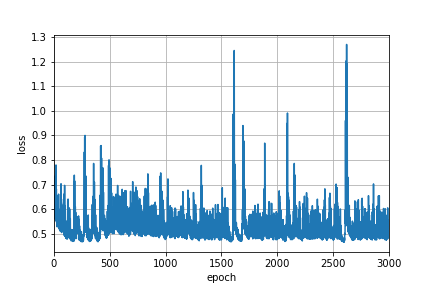
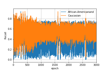
Figure 2: The plots for the loss and recall of two protected groups for each iteration during training on the COMPAS data set with equal opportunity constraints. We can see that there is some oscillation in two plots. The oscillation caused by conflicting between two constraints in (39) and violating one of them alternately shows that there is no pure equilibrium to converge to.

We also plot the loss and recalls of two protected groups for each of the iterates in Figure 2. We observe oscillation which is caused by violating constraints alternately and suggests that no pure equilibrium exists and that a stochastic classifier may be necessary. The oscillation may commonly occur in practice, especially for optimizing non-convex and non-smooth Lagrangian.

We can understand how randomized models work to achieve the fairness constraint based on this oscillation. Assume that we could find two models with the same high accuracy but different behavior on recalls. One has a high recall on black defendants, and the other has a high recall on white defendants. If we randomly select one model to make a prediction, the average result will balance the recall on two races, which leads to a fair classifier. Neural networks particularly fit this perspective, since overparameterized neural networks can represent many different but high-performing models corresponding to different parameters. We may find several candidate parameters with high accuracy but distinct prediction behaviors when adding various constraints. Then mixing candidate models indeed can improve fairness via the previous argument. The minimax optimization framework can be interpreted as an automated strategy to encourage the neural network to explore different-behavior parameters.

5 Conclusion

This work shows how to provably train neural network models under non-convex constraints via a minimax framework. Despite the difficulty of non-convex neural network models, we establish a no-regret bound for online learning of neural networks. Our results shed new light on the theoretical understanding of convergence properties of neural networks with a non-convex constrained optimization problem.

One possible avenue for future work is developing an online procedure [2, 52] for shrinkage with theoretical guarantees, which can also reduce memory costs during training. Moreover, randomized prediction violates different principles of fairness, such as “similar individuals receive similar outcomes” [34]. [25] discussed clustering and ensemble procedures to decrease randomness while satisfying the fairness defined from an individual perspective, while it may be computationally intractable for large models. It may be interesting to find more memory and computationally efficient algorithms for neural networks.

Appendix A Shrinking

From Proposition 4 we observe that a stochastic model is required to achieve a near-optimal and near-feasible solution. In our setting, the prediction model is parameterized by a neural networks, which may have a considerable amount of parameters and need a large number of iterations for training. As a result, storing all parameters for all iterations for randomized prediction may be intractable. To overcome this difficulty, it can be shown that a smaller mixed equilibrium exists and can be found by using a shrinkage procedure. In particular, let $\bm{\theta}^{1},\dots,\bm{\theta}^{t}\in\Theta$ be a sequence of $T$ iterates obtained by Algorithm 1. Define $\mathbf{c}_{0}=(h_{0}(\bm{\theta}_{1}),\dots,h_{0}(\bm{\theta}^{T}))^{\top}$ and $\mathbf{c}_{j}=(g_{j}(\mathbf{r}(\bm{\theta}^{1})),\dots,g_{j}(\mathbf{r}(\bm{\theta}^{T})))^{\top}$ for $j=1,\dots,J$. The shrinking procedure aims to solve the following linear programming problem:

$$\begin{split}\min_{\mathbf{p}\in T\text{-dimensional simplex}}&\mathbf{c}_{0}^{\top}\mathbf{p}\\ \text{s.t. }&\mathbf{c}_{j}^{\top}\mathbf{p}\leq\epsilon,\quad\text{for }j=1,\dots,J,\end{split}$$ (40)

for some $\epsilon>0$. The minimizer $\mathbf{p}^{\ast}=(p_{1}^{\ast},\dots,p_{T}^{\ast})$ of (40) represents the final stochastic classifier, with components representing the probability of sampling $\{1,\dots,T\}$. Note that due to the convexity of $g_{j}$, we have for all $j$ that

$$g_{j}\left(\sum_{t=1}^{T}p_{t}^{\ast}\mathbf{r}(\bm{\theta}^{t})\right)\leq\mathbf{c}_{j}^{\top}\mathbf{p}^{\ast}\leq\epsilon,$$

implying that the stochastic solution induced by $\mathbf{p}^{\ast}$ is near-feasible in (1) and achieves the smallest training error among all stochastic models.

[26] showed that every vertex of the feasible region and the optimal solution $\mathbf{p}^{\ast}$ have at most $J+1$ nonzero elements. That is, the shrinkage procedure selects at most $J+1$ iterations for constructing randomized solution and there are only $J+1$ non-zero elements in $\mathbf{p}^{\ast}$, which reduces memory cost significantly. Since $J$ is much smaller than $T$, heuristically, we only sample a small amount of iterates compared to $T$ in our experiment where $J$ is the number of constraints and $T$ is the total number of iterates.

Appendix B Proofs

B.1 Proof of Proposition 3

We first show that $\mathbb{E}|y(\bm{\theta}^{0};\mathbf{x})|$ is finite and then apply Markov’s inequality. Since $\|\mathbf{x}\|\leq 1$, we have

$$\mathbb{E}(\sigma((\mathbf{a}_{i}^{0})^{\top}\mathbf{x}))^{2}\leq\mathbb{E}((\mathbf{a}_{i}^{0})^{\top}\mathbf{x})^{2}\leq\mathbb{E}\|\mathbf{a}_{i}^{0}\|^{2}=1.$$ (41)

Thus, using Khintchine’s inequality (Theorem 1 in Chapter 10.3 in [24]) and the fact that $b_{i}\sim\operatorname{Uniform}(\{-1,1\})$, there exists a constant $B$ such that

$$\mathbb{E}|y(\bm{\theta}^{0};\mathbf{x})| =\mathbb{E}\left|\frac{1}{\sqrt{m}}\sum_{i=1}^{m}b_{i}\sigma((\mathbf{a}_{i}^{0})^{\top}\mathbf{x})\right|$$ (42)

$$=\mathbb{E}\left[\mathbb{E}\left|y=\frac{1}{\sqrt{m}}\sum_{i=1}^{m}b_{i}\sigma((\mathbf{a}_{i}^{0})^{\top}\mathbf{x})\right|\mid\mathbf{a}_{i}^{0},\mathbf{x}\right]$$ (43)

$$\leq\frac{B}{\sqrt{m}}\mathbb{E}\left(\sum_{i=1}^{m}(\sigma((\mathbf{a}_{i}^{0})^{\top}\mathbf{x}))^{2}\right)^{1/2} (\text{Khintchine inequality})$$ (44)

$$\leq\frac{B}{\sqrt{m}}\left(\mathbb{E}\sum_{i=1}^{m}(\sigma((\mathbf{a}_{i}^{0})^{\top}\mathbf{x}))^{2}\right)^{1/2} (\text{Jensen's inequality})$$ (45)

$$\stackrel{{\scriptstyle\eqref{eq:moment}}}{{\leq}}B.$$ (46)

Markov’s inequality implies that $\mathbb{P}(|y|>D)\leq{B}/{D}$. Moreover, we obtain

$$| y(\bm{\theta};\mathbf{x})-y(\bm{\theta}^{0};\mathbf{x})|^{2}$$ (47)

$$=\left|\frac{1}{\sqrt{m}}\sum_{i=1}^{m}b_{i}\sigma(\mathbf{a}_{i}^{\top}\mathbf{x})-\frac{1}{\sqrt{m}}\sum_{i=1}^{m}b_{i}\sigma((\mathbf{a}_{i}^{0})^{\top}\mathbf{x})\right|^{2}$$ (48)

$$\leq\sum_{i=1}^{m}\left|\sigma(\mathbf{a}_{i}^{\top}\mathbf{x})-\sigma((\mathbf{a}_{i}^{0})^{\top}\mathbf{x})\right|^{2} (\text{since }(\sum_{i=1}^{m}c_{i})^{2}\leq m\sum_{i=1}^{m}c_{i}^{2})$$ (49)

$$\leq\sum_{i=1}^{m}\left|\mathbf{a}_{i}^{\top}\mathbf{x}-(\mathbf{a}_{i}^{0})^{\top}\mathbf{x}\right|^{2} (\text{$\sigma$ is 1-Lipschitz continuous})$$ (50)

$$\leq\sum_{i=1}^{m}\|\mathbf{a}_{i}-\mathbf{a}_{i}^{0}\|^{2} (\|\mathbf{x}\|\leq 1)$$ (51)

$$\leq D^{2}.$$ (52)

The proposition follows by the triangle inequality.

B.2 Proof of Proposition 4

We prove two guarantees in Proposition 4: optimality in (23) and feasibility in (24) by properties (22) of the coarse-correlated equilibrium. First, we define $\bar{\bm{\lambda}}=\frac{1}{T}\sum_{t=1}^{T}\bm{\lambda}^{t}$ and $\bar{\bm{\xi}}=\frac{1}{T}\sum_{t=1}^{T}\bm{\xi}^{t}$.

Optimality. By Proposition 3, we have $|y(\bm{\theta};\mathbf{x})|<2D$ with probability $1-B/D$. Therefore, on the event $\{|y(\bm{\theta};\mathbf{x})|<2D\}$ we can always find a $\bm{\xi}\in\Xi$ such that $\widetilde{\mathbf{r}}(\bm{\theta})\leq\bm{\xi}$. Then, we know that the Lagrangian gives a lower bound for the original problem. That is, for any $\bm{\lambda}\geq{\bf 0}$, we have

$$\begin{split}\min_{\bm{\theta}\in\Theta,\bm{\xi}\in\Xi}\widetilde{\mathcal{L}}(\bm{\theta},\bm{\xi},\bm{\lambda})&\leq\min_{\bm{\theta}\in\Theta,\bm{\xi}\in\Xi:\mathbf{g}(\bm{\xi})\leq{\bf 0},\widetilde{\mathbf{r}}(\bm{\theta})\leq\bm{\xi}}\widetilde{\mathcal{L}}(\bm{\theta},\bm{\xi},\bm{\lambda})\\ &\leq\min_{\bm{\theta}\in\Theta,\xi\in\Xi:\mathbf{g}(\bm{\xi})\leq{\bf 0},\widetilde{\mathbf{r}}(\bm{\theta})\leq\bm{\xi}}h_{0}(\bm{\theta})\\ &=\min_{\bm{\theta}\in\Theta:\max_{j}g_{j}(\widetilde{\mathbf{r}}(\bm{\theta}))}h_{0}(\bm{\theta}),\end{split}$$ (53)

where the first inequality follows due to the fact that we restrict the search space, the second inequality holds because of $\bm{\lambda}\geq{\bf 0},\mathbf{g}(\bm{\xi})\leq{\bf 0},\widetilde{\mathbf{r}}(\bm{\theta})\leq\bm{\xi}$, and the equality follows from the monotonicity of $g_{j}$.

From the definition of the equilibrium, we obtain

$$\frac{1}{T}\sum_{t=1}^{T}\mathcal{L}(\bm{\theta}^{t},\bm{\xi}^{t},\bm{\lambda}^{t}) \stackrel{{\scriptstyle\eqref{eq:upper-bound}}}{{\leq}}\frac{1}{T}\sum_{t=1}^{T}\widetilde{\mathcal{L}}(\bm{\theta}^{t},\bm{\xi}^{t},\bm{\lambda}^{t}).$$

Using (22a) and (22b), we further have

$$\stackrel{{\scriptstyle}}{{\leq}}\min_{\bm{\xi}\in\Xi}\frac{1}{T}\sum_{t=1}^{T}\mathcal{L}_{1}(\bm{\xi},\bm{\lambda}^{t})+\epsilon_{\xi}+\min_{\bm{\theta}\in\Theta}\frac{1}{T}\sum_{t=1}^{T}\widetilde{\mathcal{L}}_{2}(\bm{\theta},\bm{\lambda}^{t})+\epsilon_{\theta}$$

$$=\min_{\bm{\theta}\in\Theta,\bm{\xi}\in\Xi}\widetilde{\mathcal{L}}(\bm{\theta},\bm{\xi},\bar{\bm{\lambda}})+\epsilon_{\theta}+\epsilon_{\xi}$$ (54)

$$\leq\min_{\bm{\theta}\in\Theta:\max_{j}g_{j}(\widetilde{\mathbf{r}}(\bm{\theta}))\leq 0}h_{0}(\bm{\theta})+\epsilon_{\theta}+\epsilon_{\xi},$$ (55)

where the equality holds due to the linearity of $\widetilde{\mathcal{L}}$ with respect to $\bm{\lambda}$, and the last line follows from $\bar{\bm{\lambda}}>{\bf 0}$ and (53).

We have for any $\bm{\lambda}^{\prime}\in\Lambda$

$$\begin{split}\frac{1}{T}\sum_{t=1}^{T}\mathcal{L}(\bm{\theta}^{t},\bm{\xi}^{t},\bm{\lambda}^{\prime})&\leq\max_{\bm{\lambda}\in\Lambda}\frac{1}{T}\sum_{t=1}^{T}\mathcal{L}(\bm{\theta}^{t},\bm{\xi}^{t},\bm{\lambda})\\ &\stackrel{{\scriptstyle\eqref{eq:OL-lambda}}}{{\leq}}\frac{1}{T}\sum_{t=1}^{T}{\mathcal{L}}(\bm{\theta}^{t},\bm{\xi}^{t},\bm{\lambda}^{t})+\epsilon_{\lambda}\\ &\stackrel{{\scriptstyle\eqref{eq:theta-xi-equilibruim}}}{{\leq}}\min_{\bm{\theta}\in\Theta:\max_{j}g_{j}(\widetilde{\mathbf{r}}(\bm{\theta}))\leq 0}h_{0}(\bm{\theta})+\epsilon_{\theta}+\epsilon_{\xi}+\epsilon_{\lambda}.\end{split}$$ (56)

The optimality follows by setting $\bm{\lambda}^{\prime}={\bf 0}$.

Feasibility. Letting $j^{\prime}\in\mathop{\mathrm{argmax}}_{j}g_{j}(\bar{\bm{\xi}})$ and setting $\lambda_{j^{\prime}}^{\prime}=\kappa$ and $\lambda^{\prime}_{j}=0$ for $j\neq j^{\prime}$, we get

$$\begin{split}\frac{1}{T}\sum_{t=1}^{T}h_{0}(\bm{\theta}^{t})+\frac{\kappa}{T}\sum_{t=1}^{T}g_{j^{\prime}}(\bm{\xi}^{t})&\stackrel{{\scriptstyle\eqref{eq:Lagrangian-1}}}{{=}}\frac{1}{T}\sum_{t=1}^{T}\mathcal{L}(\bm{\theta}^{t},\bm{\xi}^{t},\bm{\lambda}^{\prime})\\ &\stackrel{{\scriptstyle\eqref{eq:lagrangian-upper-bound}}}{{\leq}}\min_{\bm{\theta}\in\Theta:\max_{j}g_{j}(\widetilde{\mathbf{r}}(\bm{\theta}))\leq 0}h_{0}(\bm{\theta})+\epsilon_{\theta}+\epsilon_{\xi}+\epsilon_{\lambda}\end{split}$$ (57)

and, using convexity of $g_{j}$,

$$\max_{j}g_{j}(\bar{\bm{\xi}}) \leq\frac{1}{T}\sum_{t=1}^{T}g_{j^{\prime}}(\bm{\xi}^{t})$$

$$\stackrel{{\scriptstyle\eqref{eq:optimality}}}{{\leq}}\frac{1}{\kappa}\left(\min_{\bm{\theta}\in\Theta:\max_{j}g_{j}(\widetilde{\mathbf{r}}(\bm{\theta}))\leq 0}h_{0}(\bm{\theta})-\frac{1}{T}\sum_{t=1}^{T}h_{0}(\bm{\theta}^{t})+\epsilon_{\theta}+\epsilon_{\xi}+\epsilon_{\lambda}\right)$$

$$\leq\frac{2C+\epsilon_{\theta}+\epsilon_{\xi}+\epsilon_{\lambda}}{\kappa},$$ (58)

where the inequality follows from part 3 of Assumption 2. Similarly, letting $k^{\prime}\in\mathop{\mathrm{argmax}}_{k}\left(\frac{1}{T}\sum_{t}r_{k}(\bm{\theta}^{t})-\bar{\xi}_{k}\right)$ and setting $\lambda_{J+k^{\prime}}^{\prime}=\kappa$ and $\lambda_{J+k^{\prime}}=0$ for $k\neq k^{\prime}$, we obtain

$$\frac{1}{T}\sum_{t=1}^{T}h_{0}(\bm{\theta}_{t})+\kappa\left(\frac{1}{T}\sum_{t=1}^{T}r_{k^{\prime}}(\bm{\theta}^{t})-\bar{\xi}_{k^{\prime}}\right)\stackrel{{\scriptstyle\eqref{eq:Lagrangian-1}}}{{=}}\frac{1}{T}\sum_{t=1}^{T}\mathcal{L}(\bm{\theta}^{t},\bm{\xi}^{t},\bm{\lambda}^{\prime})\\ \stackrel{{\scriptstyle\eqref{eq:lagrangian-upper-bound}}}{{\leq}}\min_{\bm{\theta}\in\Theta:\max_{j}g_{j}(\widetilde{\mathbf{r}}(\bm{\theta}))\leq 0}h_{0}(\bm{\theta})+\epsilon_{\theta}+\epsilon_{\xi}+\epsilon_{\lambda},$$ (59)

which implies

$$\max_{k}\frac{1}{T}\sum_{t=1}^{T}r_{k}(\bm{\theta}^{t})-\bar{\xi}_{k}\stackrel{{\scriptstyle\eqref{eq:optimality-2}}}{{\leq}}(2C+\epsilon_{\theta}+\epsilon_{\xi}+\epsilon_{\lambda})/\kappa\\ \Longrightarrow\max_{k}\max\left\{\frac{1}{T}\sum_{t=1}^{T}r_{k}(\bm{\theta}^{t})-\bar{\xi}_{k},0\right\}\leq(2C+\epsilon_{\theta}+\epsilon_{\xi}+\epsilon_{\lambda})/\kappa.$$ (60)

Therefore, part 4 of Assumption 2 implies that

$$\max_{j}g_{j}\left(\frac{1}{T}\sum_{t=1}^{T}\mathbf{r}(\bm{\theta}^{t})\right) \leq\max_{j}g_{j}\left(\max\left\{\frac{1}{T}\sum_{t=1}^{T}\mathbf{r}(\bm{\theta}^{t})-\bar{\bm{\xi}},0\right\}+\bar{\bm{\xi}}\right)$$

as $$g_{j} g_{j}$$ is increasing. Furthermore, as is L-Lipschitz and increasing, we have

$$\leq\max_{j}g_{j}(\bar{\bm{\xi}})+L\left\|\max\left\{\frac{1}{T}\sum_{t=1}^{T}\mathbf{r}(\bm{\theta}^{t})-\bar{\bm{\xi}},0\right\}\right\|_{\infty}$$

$$=\max_{j}g_{j}(\bar{\bm{\xi}})+L\max_{k}\max\left\{\frac{1}{T}\sum_{t=1}^{T}r_{k}(\bm{\theta}^{t})-\bar{\xi}_{k},0\right\}$$

$$\leq(1+L)(2C+\epsilon_{\theta}+\epsilon_{\xi}+\epsilon_{\lambda})/\kappa,$$

where the last line follows from (58) and (60). This completes this proof.

B.3 Proof of Proposition 6

Define $\widehat{f}_{t}(\bm{\theta})=f_{t}(\bm{\theta}^{t})+(\bm{\mu}^{t})^{\top}(\bm{\theta}-\bm{\theta}^{t})$. Since $\widehat{f}_{t}(\bm{\theta})$ is convex and $\nabla\widehat{f}_{t}(\bm{\theta})=\bm{\mu}^{t}$, applying Lemma 5, we have

$$\frac{1}{T}\sum_{t=1}^{T}\widehat{f}_{t}(\bm{\theta}^{t})-\frac{1}{T}\sum_{t=1}^{T}\widehat{f}_{t}(\bm{\theta})\leq\frac{\eta W}{2}+\frac{M}{T\eta},$$ (61)

where we have used (28) and convexity of $\Theta$. We know that the convexity of $f_{t}$ implies (see, for example, [70]) the following

$$f_{t}(\bm{\theta}^{t})+\nabla f_{t}(\bm{\theta}^{t})^{\top}(\bm{\theta}-\bm{\theta}^{t})\leq f_{t}(\bm{\theta}).$$ (62)

Therefore, we have

$$\frac{1}{T}\sum_{t=1}^{T}f_{t}(\bm{\theta}^{t})-\frac{1}{T}\sum_{t=1}^{T}f_{t}(\bm{\theta})$$

$$\stackrel{{\scriptstyle\widehat{f}_{t}(\bm{\theta}^{t})=f_{t}(\bm{\theta}^{t})}}{{=}}\frac{1}{T}\sum_{t=1}^{T}\widehat{f}_{t}(\bm{\theta}^{t})-\frac{1}{T}\sum_{t=1}^{T}\widehat{f}_{t}(\bm{\theta})+\frac{1}{T}\sum_{t=1}^{T}\widehat{f}_{t}(\bm{\theta})-\frac{1}{T}\sum_{t=1}^{T}f_{t}(\bm{\theta})$$

$$\stackrel{{\scriptstyle\eqref{eq:conve-OL}}}{{\leq}}\frac{\eta W}{2}+\frac{M}{T\eta}+\frac{1}{T}\sum_{t=1}^{T}\widehat{f}_{t}(\bm{\theta})-\frac{1}{T}\sum_{t=1}^{T}f_{t}(\bm{\theta})$$

$$\stackrel{{\scriptstyle\eqref{eq:f-convex}}}{{\leq}}\frac{\eta W}{2}+\frac{M}{T\eta}+\frac{1}{T}\sum_{t=1}^{T}(\bm{\mu}^{t}-\nabla f_{t}(\bm{\theta}^{t}))^{\top}(\bm{\theta}-\bm{\theta}^{t})$$

$$=\frac{\eta W}{2}+\frac{M}{T\eta}+\frac{1}{T}\sum_{t=1}^{T}(\bm{\mu}^{t}-\nabla f_{t}(\bm{\theta}^{t})-\bm{\beta}_{t}(\bm{\theta}^{t}))^{\top}(\bm{\theta}-\bm{\theta}^{t})$$

$$\qquad\qquad+\frac{1}{T}\sum_{t=1}^{T}\bm{\beta}_{t}(\bm{\theta}^{t})^{\top}(\bm{\theta}-\bm{\theta}^{t}).$$

Since the function $h$ is differentiable and strongly convex, there exists $\bm{\theta}^{\prime}$ such that $\nabla h(\bm{\theta}^{\prime})={\bf 0}$. Thus, for all $t$, we have

$$\frac{1}{4}\|\bm{\theta}-\bm{\theta}^{t}\|^{2}\leq\frac{1}{2}\|\bm{\theta}-\bm{\theta}^{\prime}\|^{2}+\frac{1}{2}\|\bm{\theta}^{t}-\bm{\theta}^{\prime}\|^{2}\leq B_{h}(\bm{\theta},\bm{\theta}^{\prime})+B_{h}(\bm{\theta}^{t},\bm{\theta}^{\prime})\\ \stackrel{{\scriptstyle\nabla h(\bm{\theta}^{\prime})={\bf 0}}}{{\leq}}2\sup_{\bm{\theta}\in\Theta}h(\bm{\theta})\stackrel{{\scriptstyle\eqref{eq:boundedness}}}{{\leq}}2M,$$ (63)

where the first inequality holds by $(a+b)^{2}\leq 2a^{2}+2b^{2}$ and the second inequality follows by the fact that $h$ is 1-strongly convex w.r.t $\|\cdot\|$.

Using Jensen’s inequality, we have

$$\sup_{t}\|\nabla f_{t}(\bm{\theta}^{t})+\bm{\beta}_{t}(\bm{\theta}^{t})\|_{\ast}=\sup_{t}\|\mathbb{E}[\bm{\mu}^{t}|\bm{\theta}^{t}]\|_{\ast}\leq\mathbb{E}[\sup_{t}\|\bm{\mu}^{t}\|_{\ast}|\bm{\theta}^{t}]\stackrel{{\scriptstyle\eqref{eq:boundedness}}}{{\leq}}W,$$ (64)

and Holder’s inequality implies that

$$\begin{split}&\ \ \ |(\bm{\mu}^{t}-\nabla f_{t}(\bm{\theta}^{t})-\bm{\beta}_{t}(\bm{\theta}^{t}))^{\top}(\bm{\theta}-\bm{\theta}^{t})|\\ &\stackrel{{\scriptstyle\eqref{eq:theta-bound}}}{{\leq}}\|\bm{\mu}^{t}-\nabla f_{t}(\bm{\theta}^{t})-\bm{\beta}_{t}(\bm{\theta}^{t})\|_{\ast}\cdot 2\sqrt{2M}\\ &\leq(\|\bm{\mu}^{t}\|_{\ast}+\|\nabla f_{t}(\bm{\theta}^{t})+\bm{\beta}_{t}(\bm{\theta}^{t})\|_{\ast})\cdot 2\sqrt{2M}\stackrel{{\scriptstyle\eqref{eq:jensen},\eqref{eq:theta-bound}}}{{\leq}}4W\sqrt{2M}.\end{split}$$ (65)

Furthermore, due to (65) and the fact that

$$\mathbb{E}[(\bm{\mu}^{t}-\nabla f_{t}(\bm{\theta}^{t})-\bm{\beta}_{t}(\bm{\theta}^{t}))^{\top}(\bm{\theta}-\bm{\theta}^{t})|\bm{\theta}^{t}]=0,$$

$(\bm{\mu}^{t}-\nabla f_{t}(\bm{\theta}^{t})-\bm{\beta}_{t}(\bm{\theta}^{t}))^{\top}(\bm{\theta}-\bm{\theta}^{t})$ is a bounded martingale difference. Therefore, by the Hoeffding-Azuma inequality, we get

$$\mathbb{P}\left\{\sum_{t=1}^{T}(\bm{\mu}^{t}-\nabla f_{t}(\bm{\theta}^{t})-\bm{\beta}_{t}(\bm{\theta}^{t}))^{\top}(\bm{\theta}-\bm{\theta}^{t})\geq\varepsilon\right\}\leq\exp\left(\frac{-\varepsilon^{2}}{64TW^{2}M}\right).$$

The proposition follows by setting $\varepsilon=8W\sqrt{TM\log(1/\delta)}$ and $\eta=\sqrt{\frac{M}{TW}}$.

B.4 Proof of Proposition 8

Since $\|\mathbf{x}\|_{2}\leq 1$ and $b_{i}\in\{-1,1\}$, we have $\|\nabla y(\bm{\theta};\mathbf{x})\|_{2}\leq 1$ as

$$\nabla y(\bm{\theta};\mathbf{x})=\frac{1}{\sqrt{m}}\left(\operatorname*{1{\hskip-2.5pt}\hbox{$\rm{I}$}}\{\mathbf{a}_{1}^{\top}\mathbf{x}>0\}\mathbf{x}^{\top},\dots,\operatorname*{1{\hskip-2.5pt}\hbox{$\rm{I}$}}\{\mathbf{a}_{m}^{\top}\mathbf{x}>0\}\mathbf{x}^{\top}\right)^{\top}.$$ (66)

Following [54], we prove the local linearization for neural network models. Given $\mathbf{x}\in\mathcal{X}$ and a layer $i$ such that $\operatorname*{1{\hskip-2.5pt}\hbox{$\rm{I}$}}\{\mathbf{a}_{i}^{\top}\mathbf{x}>0\}\neq\operatorname*{1{\hskip-2.5pt}\hbox{$\rm{I}$}}\{(\mathbf{a}_{i}^{0})^{\top}\mathbf{x}>0\}$, applying the Cauchy–Schwarz inequality gives us

$$\quad\quad(\mathbf{a}_{i}^{\top}\mathbf{x})((\mathbf{a}_{i}^{0})^{\top}\mathbf{x})<0$$ (67a)

$$\Longrightarrow|(\mathbf{a}_{i}^{0})^{\top}\mathbf{x}|\stackrel{{\scriptstyle\eqref{eq:cond1}}}{{\leq}}|(\mathbf{a}_{i}^{0}-\mathbf{a}_{i})^{\top}\mathbf{x}|\stackrel{{\scriptstyle\|\mathbf{x}\|_{2}\leq 1}}{{\leq}}\|\mathbf{a}_{i}^{0}-\mathbf{a}_{i}\|_{2}.$$ (67b)

Thus, we get

$$\begin{split}&\ \ \ |y(\bm{\theta};\mathbf{x})-y^{0}(\bm{\theta};\mathbf{x})|\\ &=\frac{1}{\sqrt{m}}\left|\sum_{i=1}^{m}b_{i}(\operatorname*{1{\hskip-2.5pt}\hbox{$\rm{I}$}}\{\mathbf{a}_{i}^{\top}\mathbf{x}>0\}-\operatorname*{1{\hskip-2.5pt}\hbox{$\rm{I}$}}\{(\mathbf{a}_{i}^{0})^{\top}\mathbf{x}>0\})\mathbf{a}_{i}^{\top}\mathbf{x}\right|\\ &\stackrel{{\scriptstyle\|\mathbf{x}\|_{2}\leq 1}}{{\leq}}\frac{1}{\sqrt{m}}\sum_{i=1}^{m}\left|\operatorname*{1{\hskip-2.5pt}\hbox{$\rm{I}$}}\{\mathbf{a}_{i}^{\top}\mathbf{x}>0\}-\operatorname*{1{\hskip-2.5pt}\hbox{$\rm{I}$}}\{(\mathbf{a}_{i}^{0})^{\top}\mathbf{x}>0\}\right|(|(\mathbf{a}_{i}^{0})^{\top}\mathbf{x}|+\|\mathbf{a}_{i}-\mathbf{a}_{i}^{0}\|_{2})\\ &\stackrel{{\scriptstyle\eqref{eq:ind}}}{{\leq}}\frac{1}{\sqrt{m}}\sum_{i=1}^{m}\operatorname*{1{\hskip-2.5pt}\hbox{$\rm{I}$}}\{|(\mathbf{a}_{i}^{0})^{\top}\mathbf{x}|\leq\|\mathbf{a}_{i}^{0}-\mathbf{a}_{i}\|_{2}\}(|(\mathbf{a}_{i}^{0})^{\top}x|+\|\mathbf{a}_{i}-\mathbf{a}_{i}^{0}\|_{2})\\ &\leq\frac{2}{\sqrt{m}}\sum_{i=1}^{m}\operatorname*{1{\hskip-2.5pt}\hbox{$\rm{I}$}}\{|(\mathbf{a}_{i}^{0})^{\top}\mathbf{x}|\leq\|\mathbf{a}_{i}^{0}-\mathbf{a}_{i}\|_{2}\}\|\mathbf{a}_{i}-\mathbf{a}_{i}^{0}\|_{2},\end{split}$$ (68)

where we have used $\operatorname*{1{\hskip-2.5pt}\hbox{$\rm{I}$}}\{|c|\leq d\}|c|\leq\operatorname*{1{\hskip-2.5pt}\hbox{$\rm{I}$}}\{|c|\leq d\}d$ for the last inequality.

For $v\sim\chi_{d}^{2}$, where $\chi^{2}_{d}$ denotes a chi-squared distribution with $d$ degrees of freedom, we have $\mathbb{E}[1/v]=1/(\text{deg}-2)$. Therefore, we have

$$\mathbb{E}\|\mathbf{a}_{i}^{0}\|_{2}^{-2}=\frac{1}{d-2}.$$ (69)

Furthermore, applying Cauchy–Schwarz inequality (68), we get

$$\mathbb{E}_{\mathbf{x},\bm{\theta}^{0}} |y(\bm{\theta};\mathbf{x})-y^{0}(\bm{\theta};\mathbf{x})|^{2}$$ (70)

$$\leq\frac{4}{m}\mathbb{E}_{\mathbf{x},\bm{\theta}^{0}}\left(\sum_{i=1}^{m}\operatorname*{1{\hskip-2.5pt}\hbox{$\rm{I}$}}\{|(\mathbf{a}_{i}^{0})^{\top}x|\leq\|\mathbf{a}_{i}^{0}-\mathbf{a}_{i}\|_{2}\}\right)\left(\sum_{i=1}^{m}\|\mathbf{a}_{i}-\mathbf{a}_{i}^{0}\|_{2}^{2}\right).$$ (71)

Since $$\|\bm{\theta}-\bm{\theta}^{0}\|_{2}\leq D$$, we further have

$$\leq\frac{4D^{2}}{m}\sum_{i=1}^{m}\mathbb{E}_{\mathbf{x},\bm{\theta}^{0}}\operatorname*{1{\hskip-2.5pt}\hbox{$\rm{I}$}}\{|(\mathbf{a}_{i}^{0})^{\top}\mathbf{x}|\leq\|\mathbf{a}_{i}^{0}-\mathbf{a}_{i}\|_{2}\}.$$ (72)

Using Part 2 in Assumption 7 and the Cauchy–Schwarz inequality again, we have

$$\leq\frac{4cD^{2}}{m}\mathbb{E}_{\bm{\theta}^{0}}\left[\sum_{i=1}^{m}\frac{\|\mathbf{a}_{i}^{0}-\mathbf{a}_{i}\|_{2}}{\|\mathbf{a}_{i}^{0}\|_{2}}\right]$$ (73)

$$\leq\frac{4cD^{2}}{m}\mathbb{E}_{\bm{\theta}^{0}}\left(\sum_{i=1}^{m}\|\mathbf{a}_{i}^{0}\|_{2}^{-2}\right)^{1/2}\left(\sum_{i=1}^{m}\|\mathbf{a}_{i}^{0}-\mathbf{a}_{i}\|_{2}^{2}\right)^{1/2}.$$ (74)

Using $$\|\bm{\theta}-\bm{\theta}^{0}\|_{2}\leq D$$ we have

$$\leq\frac{4cD^{3}}{m}\left(\sum_{i=1}^{m}\mathbb{E}_{\bm{\theta}^{0}}\|\mathbf{a}_{i}^{0}\|_{2}^{-2}\right)^{1/2}$$ (75)

$$=\frac{4cD^{3}}{m^{1/2}(d-2)^{1/2}},$$ (76)

where we have used Jensen’s inequality for the square root function, expectation in the second to last inequality, and (69) at the end. Following a similar argument, we have

$$\mathbb{E}_{\mathbf{x},\bm{\theta}^{0}} \|\nabla y(\bm{\theta};\mathbf{x})-\nabla y^{0}(\bm{\theta};\mathbf{x})\|_{2}$$

$$\stackrel{{\scriptstyle\eqref{eq:grad-y}}}{{=}}\frac{1}{m}\mathbb{E}_{\mathbf{x},\bm{\theta}^{0}}\left\|\sum_{i=1}^{m}b_{i}(\operatorname*{1{\hskip-2.5pt}\hbox{$\rm{I}$}}\{\mathbf{a}_{i}^{\top}\mathbf{x}>0\}-\operatorname*{1{\hskip-2.5pt}\hbox{$\rm{I}$}}\{(\mathbf{a}_{i}^{0})^{\top}\mathbf{x}>0\})\mathbf{x}\right\|_{2}$$

$$\stackrel{{\scriptstyle\eqref{eq:ind}}}{{\leq}}\frac{1}{m}\mathbb{E}_{\mathbf{x},\bm{\theta}^{0}}\sum_{i=1}^{m}\operatorname*{1{\hskip-2.5pt}\hbox{$\rm{I}$}}\{|(\mathbf{a}_{i}^{0})^{\top}\mathbf{x}|\leq\|\mathbf{a}_{i}^{0}-\mathbf{a}_{i}\|_{2}\}\|\mathbf{x}\|_{2}$$

$$\leq\frac{1}{m}\mathbb{E}_{\mathbf{x},\bm{\theta}^{0}}\sum_{i=1}^{m}\operatorname*{1{\hskip-2.5pt}\hbox{$\rm{I}$}}\{|(\mathbf{a}_{i}^{0})^{\top}\mathbf{x}|\leq\|\mathbf{a}_{i}^{0}-\mathbf{a}_{i}\|_{2}\}.$$

Using $$\|\mathbf{x}\|_{2}\leq 1$$ and part 2 in Assumption 7, we have

$$\leq\frac{c}{m}\mathbb{E}_{\bm{\theta}^{0}}\sum_{i=1}^{m}\frac{\|\mathbf{a}_{i}^{0}-\mathbf{a}_{i}\|_{2}}{\|\mathbf{a}_{i}^{0}\|_{2}}$$

$$\leq\frac{Dc}{m}\left(\sum_{i=1}^{m}\mathbb{E}_{\bm{\theta}^{0}}\|\mathbf{a}_{i}^{0}\|_{2}^{-2}\right)^{1/2}$$

$$\stackrel{{\scriptstyle\eqref{eq:inverse-chi-squared distribution}}}{{=}}\frac{Dc}{m^{1/2}(d-2)^{1/2}},$$

where the last inequality follows from Cauchy–Schwarz inequality, $\|\bm{\theta}-\bm{\theta}^{0}\|_{2}\leq D$, and Jensen’s inequality. This completes the proof.

B.5 Proof of Theorem 9

From the decomposition (33), it suffices to bound three terms $(I),(III),(III)$. The $(I)$ and $(III)$ in (33) can be bounded in a uniform manner. Note that $y^{0}$ depends on $\bm{\theta}^{0}$. In particular, given any $\bm{\theta}\in\Theta$, since $f_{t}$ is convex for all $t$, we have that

$$\mathbb{E}_{\mathbf{x},z,\bm{\theta}^{0}} \left[f_{t}(y(\bm{\theta};\mathbf{x}),z)-f_{t}(y^{0}(\bm{\theta};\mathbf{x}),z)\right]$$ (77)

$$\stackrel{{\scriptstyle}}{{\leq}}\sup_{t,y,z}|\nabla_{y}f_{t}(y,z)|\times\mathbb{E}_{\mathbf{x},\bm{\theta}^{0}}|(y(\bm{\theta};\mathbf{x})-y^{0}(\bm{\theta};\mathbf{x}))|$$ (78)

$$\stackrel{{\scriptstyle\eqref{eq:thm-asp}}}{{\leq}}L_{f}\mathbb{E}_{x,\bm{\theta}^{0}}|y(\bm{\theta}^{t};\mathbf{x})-y^{0}(\bm{\theta}^{t};\mathbf{x})|.$$ (79)

Using Jensen’s Inequality and Part 2 in Proposition 8, we have

$$\stackrel{{\scriptstyle}}{{\leq}}L_{f}\left(\mathbb{E}_{x,\bm{\theta}^{0}}|(y(\bm{\theta}^{t};\mathbf{x})-y^{0}(\bm{\theta}^{t};\mathbf{x}))|^{2}\right)^{1/2}$$ (80)

$$\stackrel{{\scriptstyle}}{{=}}O\left(\frac{L_{f}D^{3/2}}{m^{1/4}}\right).$$ (81)

This implies that

$$\begin{split}(III)&=\frac{1}{T}\sum_{t=1}^{T}\mathbb{E}_{\mathbf{x},z,\bm{\theta}^{0}}[f_{t}(y^{0}(\bm{\theta};\mathbf{x}),z)]-\frac{1}{T}\sum_{t=1}^{T}\mathbb{E}_{\mathbf{x},z,\bm{\theta}^{0}}[f_{t}(y(\bm{\theta};\mathbf{x}),z)]\\ &\leq\left|\frac{1}{T}\sum_{t=1}^{T}\mathbb{E}_{\mathbf{x},z,\bm{\theta}^{0}}[f_{t}(y^{0}(\bm{\theta};\mathbf{x}),z)]-\frac{1}{T}\sum_{t=1}^{T}\mathbb{E}_{\mathbf{x},z,\bm{\theta}^{0}}[f_{t}(y(\bm{\theta};\mathbf{x}),z)]\right|\\ &\stackrel{{\scriptstyle}}{{\leq}}\sup_{t}\mathbb{E}_{\mathbf{x},z,\bm{\theta}^{0}}|[f_{t}(y^{0}(\bm{\theta};\mathbf{x}),z)]-f_{t}(y(\bm{\theta};\mathbf{x}),z)|.\end{split}$$ (82)

The term $(I)$ is controlled in a similar manner, and we get

$$(I)=O\left(\frac{L_{f}D^{3/2}}{m^{1/4}}\right),\ \ \ (III)=O\left(\frac{L_{f}D^{3/2}}{m^{1/4}}\right).$$

To apply Proposition 6 for the second term $(II)$, let $h(\bm{\theta})=\frac{1}{2}\|\bm{\theta}-\bm{\theta}^{0}\|^{2}$. Then, $h^{\ast}(\bm{\theta})=\frac{1}{2}\|\bm{\theta}\|^{2}+\bm{\theta}^{\top}\bm{\theta}^{0}$, $B_{h}(\bm{\theta},\bm{\theta}^{\prime})=\frac{1}{2}\|\bm{\theta}-\bm{\theta}^{\prime}\|^{2}$, and (27) reduces to Algorithm 1. We have $\sup_{\bm{\theta}\in\Theta}h(\bm{\theta})=M\leq D^{2}/2$. Then, it suffices to show $\sup_{t}\|\bm{\mu}^{t}\|_{2}=W<L_{f}$, where $\bm{\mu}^{t}=\nabla f_{t}(y(\bm{\theta}^{t};\mathbf{x}_{t+1}),z_{t+1})$,

$$\mathbb{E}\left[\bm{\mu}^{t}\mid\bm{\theta}^{t}\right]=\mathbb{E}_{x,z,\bm{\theta}^{0}}[\nabla f_{t}(y^{0}(\bm{\theta}^{t};\mathbf{x}),z)\mid\bm{\theta}^{t}]+\bm{\beta}_{t}(\bm{\theta}^{t}),$$ (83)

and

$$\bm{\beta}_{t}(\bm{\theta}^{t})=\mathbb{E}_{x,z,\bm{\theta}^{0}}[\nabla f_{t}(y(\bm{\theta}^{t};\mathbf{x}),z)-\nabla f_{t}(y^{0}(\bm{\theta}^{t};\mathbf{x}),z)\mid\bm{\theta}^{t}].$$ (84)

We have

$$\sup_{t}\|\bm{\mu}^{t}\|_{2} =\sup_{t}\|\nabla f_{t}(y(\bm{\theta}^{t};\mathbf{x}_{t+1}),z_{t+1})\|_{2}$$

$$=\sup_{t}\|\nabla_{y}f_{t}(y(\bm{\theta}^{t};\mathbf{x}_{t+1}),z_{t+1})\nabla_{\bm{\theta}}y(\bm{\theta}^{t};\mathbf{x}_{t+1})\|_{2},$$

which can further be bounded using Part 1 in Proposition 8 as

$$\stackrel{{\scriptstyle}}{{\leq}}\sup_{t,y\in\mathcal{Y},z\in\mathcal{Z}}|\nabla_{y}f_{t}(y,z)|$$

$$\stackrel{{\scriptstyle\eqref{eq:thm-asp}}}{{\leq}}L_{f}.$$

Applying Proposition 6 with $\eta=\sqrt{\frac{M}{TW}}=\sqrt{\frac{D^{2}}{2L_{f}T}}$, we get

$$(II) =\frac{1}{T}\sum_{t=1}^{T}\mathbb{E}_{x,z,\bm{\theta}^{0}}[f_{t}(y^{0}(\bm{\theta}^{t};\mathbf{x}),z)]-\frac{1}{T}\sum_{t=1}^{T}\mathbb{E}_{x,z,\bm{\theta}^{0}}[f_{t}(y^{0}(\bm{\theta};\mathbf{x}),z)]$$

$$\leq\frac{3}{2}\sqrt{\frac{MW}{T}}+8W\sqrt{\frac{M\ln(1/\delta)}{T}}+\frac{2\sqrt{2M}}{T}\sum_{t=1}^{T}\|\bm{\beta}_{t}(\bm{\theta}^{t})\|_{2}$$

$$=\frac{3D}{2}\sqrt{\frac{L_{f}}{2T}}+8L_{f}D\sqrt{\frac{\ln(1/\delta)}{2T}}+\frac{2D}{T}\sum_{t=1}^{T}\|\beta_{t}(\bm{\theta}^{t})\|_{2},$$

with probability $1-\delta$. Furthermore, using Jensen’s inequality, we have

$$\|\bm{\beta}_{t}(\bm{\theta})\|_{2} \stackrel{{\scriptstyle\text{ }}}{{\leq}}\mathbb{E}_{x,z,\bm{\theta}^{0}}\|\nabla f_{t}(y(\bm{\theta};\mathbf{x}),z)-\nabla f_{t}(y^{0}(\bm{\theta};\mathbf{x}),z)\|_{2}$$

$$=\mathbb{E}_{x,z,\bm{\theta}^{0}}\|\nabla_{y}f_{t}(y(\bm{\theta};\mathbf{x}),z)\nabla_{\bm{\theta}}y(\bm{\theta};\mathbf{x})-\nabla_{y}f_{t}(y^{0}(\bm{\theta};\mathbf{x}),z)\nabla_{\bm{\theta}}y^{0}(\bm{\theta};\mathbf{x})\|_{2}$$

$$\leq\mathbb{E}_{x,z,\bm{\theta}^{0}}|\nabla_{y}f_{t}(y(\bm{\theta};\mathbf{x}),z)-\nabla_{y}f_{t}(y^{0}(\bm{\theta};\mathbf{x}),z)|\|\nabla_{\bm{\theta}}y(\bm{\theta};\mathbf{x})\|_{2}$$

$$\quad+\mathbb{E}_{x,z,\bm{\theta}^{0}}|\nabla f_{t}(y^{0}(\bm{\theta};\mathbf{x}),z)|\|\nabla_{\bm{\theta}}y(\bm{\theta};\mathbf{x})-\nabla_{\bm{\theta}}y^{0}(\bm{\theta};\mathbf{x})\|_{2},$$

which can further be bounded by Part 1 in Proposition 8 as

$$\leq\mathbb{E}_{x,z,\bm{\theta}^{0}}|\nabla_{y}f_{t}(y(\bm{\theta};\mathbf{x}),z)-\nabla_{y}f_{t}(y^{0}(\bm{\theta};\mathbf{x}),z)|$$

$$\qquad\qquad+\mathbb{E}_{x,z,\bm{\theta}^{0}}|\nabla f_{t}(y^{0}(\bm{\theta};\mathbf{x}),z)|\|\nabla_{\bm{\theta}}y(\bm{\theta};\mathbf{x})-\nabla_{\bm{\theta}}y^{0}(\bm{\theta};\mathbf{x})\|_{2}$$

$$\stackrel{{\scriptstyle\eqref{eq:thm-asp}}}{{\leq}}2L_{f}^{2}(\mathbb{E}_{x,z,\bm{\theta}^{0}}|y(\bm{\theta}^{t};\mathbf{x})-y^{0}(\bm{\theta}^{t};\mathbf{x})|$$

$$\qquad\qquad+\mathbb{E}_{x,z,\bm{\theta}^{0}}\|\nabla_{\bm{\theta}}y(\bm{\theta}^{t};\mathbf{x})-\nabla_{\bm{\theta}}y^{0}(\bm{\theta}^{t};\mathbf{x})\|_{2})$$

$$\stackrel{{\scriptstyle}}{{=}}O\left(L_{f}^{2}\left[\frac{D^{3/2}}{m^{1/4}}+\frac{D}{m^{1/2}}\right]\right)=O\left(\frac{L_{f}^{2}D^{3/2}}{m^{1/4}}\right),$$

where we used (81) and Parts 2 and 3 in Proposition 8 at the end. Combining all the results, we get

$$\begin{split}\frac{1}{T}\sum_{t=1}^{T}&\mathbb{E}_{x,z,\bm{\theta}^{0}}[f_{t}(y^{0}(\bm{\theta}^{t};\mathbf{x}),z)]-\min_{\theta}\frac{1}{T}\sum_{t=1}^{T}\mathbb{E}_{x,z,\bm{\theta}^{0}}[f_{t}(y^{0}(\bm{\theta};\mathbf{x}),z)]\\ &=O\left(D\sqrt{\frac{L_{f}}{T}}+L_{f}D\sqrt{\frac{\ln(1/\delta)}{T}}+\frac{L_{f}^{2}D^{3/2}}{m^{1/4}}\right),\end{split}$$

which finishes the proof.

B.6 Proof of Theorem 11

Since (37) and (38) immediately follow by Proposition 4, it suffices to prove the regret bounds in (36). For $\bm{\theta}$, we will use the result in Theorem 9 and justify its conditions. For $\bm{\xi}$ and $\bm{\lambda}$, we could apply Proposition 6, because their objective functions are convex.

We first prove that $\bm{\theta}^{t}$ achieves its approximate coarse-correlated equilibrium in (22b). It suffices to verify condition (35) in Theorem 9, and that the boundedness condition is satisfied by the assumption on $\Theta$ in the first statement in Assumption 2 by letting $h(\bm{\theta})=\frac{1}{2}\|\bm{\theta}-\bm{\theta}^{0}\|^{2}$. Let

$$f_{t}(y,z)=h_{0}(y,z)+\sum_{k=1}^{K}\lambda_{J+k}^{t}\widetilde{h}_{k}(y,z).$$ (85)

By Assumption 10, we have

$$\begin{split}|\nabla_{y}f_{t}(y,x)|\leq\left|\nabla_{y}h_{0}(y,z)\right|+\sum_{k=1}^{K}\lambda_{J+k}^{t}\left|\nabla_{y}\widetilde{h}_{k}(y,z)\right|=(1+K\kappa)L\leq 2K\kappa L\end{split}$$

and

$$\begin{split}|\nabla_{y}&f_{t}(y_{1},x)-\nabla_{y}f_{t}(y_{2},x)|\\ &\leq\left|\nabla_{y}h_{0}(y_{1},z)-\nabla_{y}h_{0}(y_{2},z)\right|+\sum_{k=1}^{K}\lambda_{J+k}^{t}\left|\nabla_{y}\widetilde{h}_{k}(y_{1},z)-\nabla_{y}\widetilde{h}_{k}(y_{2},z)\right|\\ &=(1+K\kappa)L|y_{1}-y_{2}|\leq 2KL\kappa|y_{1}-y_{2}|.\end{split}$$

Therefore, using Theorem 9, with probability $1-\delta$ and $\eta_{\theta}=\sqrt{D^{2}/[4K\kappa LT]}$, we have

$$\frac{1}{T}\sum_{t=1}^{T}\widetilde{\mathcal{L}}_{2}(\bm{\theta}^{t},\bm{\lambda}^{t})-\min_{\bm{\theta}\in\Theta}\frac{1}{T}\sum_{t=1}^{T}\widetilde{\mathcal{L}}_{2}(\bm{\theta},\bm{\lambda}^{t})\\ =O\left(KL\kappa D\sqrt{\frac{\ln(1/\delta)}{T}}+\frac{(KL\kappa)^{2}D^{3/2}}{m^{1/4}}\right),$$

which proves (22b) with

$$\epsilon_{\theta}=O\left(\kappa D\sqrt{\frac{\ln(1/\delta)}{T}}+\frac{\kappa^{2}D^{3/2}}{m^{1/4}}\right).$$ (86)

Then, we prove (22a) for $\bm{\xi}$. Note that Proposition 3 implies that

$$\sup_{\bm{\theta}\in\Theta}|y(\bm{\theta};\mathbf{x})|<2D$$

with probability $1-B/D$. On the event $\sup_{\bm{\theta}\in\Theta}y(\bm{\theta};\mathbf{x})\in\mathcal{Y}=\{y:|y|<2D\}$, Assumption 10 implies

$$\begin{split}&\ \ \sup_{t}\|\nabla_{\bm{\xi}}\mathcal{L}_{1}(\bm{\xi}^{t},\bm{\lambda}^{t})\|_{2}\\ &\leq\sup_{t,\bm{\xi}\in\Xi,\bm{\lambda}\in\Lambda}\left\|\left(\sum_{j=1}^{J}\lambda_{j}\nabla_{\xi_{1}}g_{j}(\bm{\xi})-\lambda_{J+1},\dots,\sum_{j=1}^{J}\lambda_{j}\nabla_{\xi_{K}}g_{j}(\bm{\xi})-\lambda_{J+K}\right)^{\top}\right\|_{2}\\ &\leq\sup_{t,\bm{\xi}\in\Xi,\bm{\lambda}\in\Lambda}\sum_{k=1}^{K}\left|\sum_{j=1}^{J}\lambda_{j}\nabla_{\xi_{k}}g_{j}(\bm{\xi})-\lambda_{J+k}\right|\\ &\leq\kappa K(JL+1)\leq 2\kappa JLK.\end{split}$$

By Assumption 2, we know $\sup_{y\in\mathcal{Y},z\in\mathcal{Z}}|\widetilde{h}_{k}|\leq C$. Thus, Proposition 6 with $M=C\sqrt{K},W=2\kappa JLK$ implies

$$\frac{1}{T}\sum_{t=1}^{T}\mathcal{L}_{1}(\bm{\xi}^{t},\bm{\lambda}^{t})-\min_{\bm{\xi}\in\Xi}\frac{1}{T}\sum_{t=1}^{T}\mathcal{L}_{1}(\bm{\xi},\bm{\lambda}^{t})=O\left(\kappa JLK^{5/4}\sqrt{\frac{C\ln(1/\delta)}{T}}\right),$$ (87)

with probability $1-\delta$ and $\eta_{\xi}=\sqrt{\frac{C}{2T\kappa JLK^{1/2}}}$. Therefore, (22a) follows with

$$\epsilon_{\xi}=O\left(\frac{\kappa\sqrt{\ln(1/\delta)}}{\sqrt{T}}\right).$$ (88)

Finally, we prove that $\bm{\lambda}^{t}$ satisfies (22c). We have

$$\begin{split}\sup_{t}&\|\widehat{\nabla}_{\bm{\lambda}}\mathcal{L}(\bm{\theta}^{t},\bm{\xi}^{t},\bm{\lambda}^{t})\|_{2}\\ &=\sup_{\bm{\theta}\in\Theta,\bm{\xi}\in\Xi}\|(g_{1}(\bm{\xi}),\dots,g_{J}(\bm{\xi}))^{\top}\|_{2}\\ &\qquad\qquad+\sup_{\bm{\theta}\in\Theta,\bm{\xi}\in\Xi}\|\{h_{j}(y(\bm{\theta};\mathbf{x}_{t+1,j}),z_{t+1,j})-\xi_{j}\}_{j=1}^{K}\|_{2}\\ &\leq JC+2KC\leq 2KJCL\end{split}$$

by Assumption 2 and $\|\bm{\lambda}^{t}\|_{2}\leq\kappa\sqrt{K+J}\leq\kappa\sqrt{KJ}$. Using Proposition 6 with $M=\kappa\sqrt{KJ},W=2KJCL$, we get

$$\frac{1}{T}\sum_{t=1}^{T}\mathcal{L}(\bm{\theta}^{t},\bm{\xi}^{t},\bm{\lambda}^{t})-\min_{\bm{\lambda}\in\Lambda}\frac{1}{T}\sum_{t=1}^{T}\mathcal{L}(\bm{\theta}^{t},\bm{\xi}^{t},\bm{\lambda})=O\left(K^{5/4}J^{5/4}CL\sqrt{\frac{\kappa\ln(1/\delta)}{T}}\right),$$

with probability $1-\delta$, which implies (22c) with

$$\epsilon_{\lambda}=O\left(\sqrt{\frac{\kappa\ln(1/\delta)}{T}}\right),$$

by setting $\eta_{\lambda}=\sqrt{\kappa/(2LCK^{1/2}J^{1/2}T)}$.

The theorem follows by the union bound.

References

• [1] {binproceedings}[author] \bauthor\bsnmAgarwal, \bfnmAlekh\binitsA., \bauthor\bsnmBeygelzimer, \bfnmAlina\binitsA., \bauthor\bsnmDudik, \bfnmMiroslav\binitsM., \bauthor\bsnmLangford, \bfnmJohn\binitsJ. and \bauthor\bsnmWallach, \bfnmHanna\binitsH. (\byear2018). \btitleA Reductions Approach to Fair Classification. In \bbooktitleProceedings of the 35th International Conference on Machine Learning (\beditor\bfnmJennifer\binitsJ. \bsnmDy and \beditor\bfnmAndreas\binitsA. \bsnmKrause, eds.). \bseriesProceedings of Machine Learning Research \bvolume80 \bpages60–69. \bpublisherPMLR. \endbibitem
• [2] {barticle}[author] \bauthor\bsnmAgrawal, \bfnmShipra\binitsS., \bauthor\bsnmWang, \bfnmZizhuo\binitsZ. and \bauthor\bsnmYe, \bfnmYinyu\binitsY. (\byear2014). \btitleA Dynamic Near-Optimal Algorithm for Online Linear Programming. \bjournalOperations Research \bvolume62 \bpages876–890. \bdoi10.1287/opre.2014.1289 \endbibitem
• [3] {binproceedings}[author] \bauthor\bsnmAlemohammad, \bfnmSina\binitsS., \bauthor\bsnmWang, \bfnmZichao\binitsZ., \bauthor\bsnmBalestriero, \bfnmRandall\binitsR. and \bauthor\bsnmBaraniuk, \bfnmRichard\binitsR. (\byear2021). \btitleThe Recurrent Neural Tangent Kernel. In \bbooktitleInternational Conference on Learning Representations. \endbibitem
• [4] {binproceedings}[author] \bauthor\bsnmAllen-Zhu, \bfnmZeyuan\binitsZ. and \bauthor\bsnmLi, \bfnmYuanzhi\binitsY. (\byear2019). \btitleWhat Can ResNet Learn Efficiently, Going Beyond Kernels? In \bbooktitleAdvances in Neural Information Processing Systems (\beditor\bfnmH.\binitsH. \bsnmWallach, \beditor\bfnmH.\binitsH. \bsnmLarochelle, \beditor\bfnmA.\binitsA. \bsnmBeygelzimer, \beditor\bfnmF.\binitsF. \bparticled' \bsnmAlché-Buc, \beditor\bfnmE.\binitsE. \bsnmFox and \beditor\bfnmR.\binitsR. \bsnmGarnett, eds.) \bvolume32. \bpublisherCurran Associates, Inc. \endbibitem
• [5] {binproceedings}[author] \bauthor\bsnmAllen-Zhu, \bfnmZeyuan\binitsZ., \bauthor\bsnmLi, \bfnmYuanzhi\binitsY. and \bauthor\bsnmLiang, \bfnmYingyu\binitsY. (\byear2019). \btitleLearning and Generalization in Overparameterized Neural Networks, Going Beyond Two Layers. In \bbooktitleAdvances in Neural Information Processing Systems (\beditor\bfnmH.\binitsH. \bsnmWallach, \beditor\bfnmH.\binitsH. \bsnmLarochelle, \beditor\bfnmA.\binitsA. \bsnmBeygelzimer, \beditor\bfnmF.\binitsF. \bparticled' \bsnmAlché-Buc, \beditor\bfnmE.\binitsE. \bsnmFox and \beditor\bfnmR.\binitsR. \bsnmGarnett, eds.) \bvolume32. \bpublisherCurran Associates, Inc. \endbibitem
• [6] {binproceedings}[author] \bauthor\bsnmAllen-Zhu, \bfnmZeyuan\binitsZ., \bauthor\bsnmLi, \bfnmYuanzhi\binitsY. and \bauthor\bsnmSong, \bfnmZhao\binitsZ. (\byear2019). \btitleA Convergence Theory for Deep Learning via Over-Parameterization. In \bbooktitleProceedings of the 36th International Conference on Machine Learning (\beditor\bfnmKamalika\binitsK. \bsnmChaudhuri and \beditor\bfnmRuslan\binitsR. \bsnmSalakhutdinov, eds.). \bseriesProceedings of Machine Learning Research \bvolume97 \bpages242–252. \bpublisherPMLR. \endbibitem
• [7] {binproceedings}[author] \bauthor\bsnmAllen-Zhu, \bfnmZeyuan\binitsZ., \bauthor\bsnmLi, \bfnmYuanzhi\binitsY. and \bauthor\bsnmSong, \bfnmZhao\binitsZ. (\byear2019). \btitleOn the Convergence Rate of Training Recurrent Neural Networks. In \bbooktitleAdvances in Neural Information Processing Systems (\beditor\bfnmH.\binitsH. \bsnmWallach, \beditor\bfnmH.\binitsH. \bsnmLarochelle, \beditor\bfnmA.\binitsA. \bsnmBeygelzimer, \beditor\bfnmF.\binitsF. \bparticled' \bsnmAlché-Buc, \beditor\bfnmE.\binitsE. \bsnmFox and \beditor\bfnmR.\binitsR. \bsnmGarnett, eds.) \bvolume32. \bpublisherCurran Associates, Inc. \endbibitem
• [8] {binproceedings}[author] \bauthor\bsnmArora, \bfnmSanjeev\binitsS., \bauthor\bsnmDu, \bfnmSimon\binitsS., \bauthor\bsnmHu, \bfnmWei\binitsW., \bauthor\bsnmLi, \bfnmZhiyuan\binitsZ. and \bauthor\bsnmWang, \bfnmRuosong\binitsR. (\byear2019). \btitleFine-Grained Analysis of Optimization and Generalization for Overparameterized Two-Layer Neural Networks. In \bbooktitleProceedings of the 36th International Conference on Machine Learning (\beditor\bfnmKamalika\binitsK. \bsnmChaudhuri and \beditor\bfnmRuslan\binitsR. \bsnmSalakhutdinov, eds.). \bseriesProceedings of Machine Learning Research \bvolume97 \bpages322–332. \bpublisherPMLR. \endbibitem
• [9] {barticle}[author] \bauthor\bsnmBa, \bfnmJimmy Lei\binitsJ. L., \bauthor\bsnmKiros, \bfnmJamie Ryan\binitsJ. R. and \bauthor\bsnmHinton, \bfnmGeoffrey E\binitsG. E. (\byear2016). \btitleLayer normalization. \bjournalarXiv preprint arXiv:1607.06450. \endbibitem
• [10] {barticle}[author] \bauthor\bsnmBauschke, \bfnmHeinz H\binitsH. H., \bauthor\bsnmBorwein, \bfnmJonathan M\binitsJ. M. \betalet al. (\byear1997). \btitleLegendre functions and the method of random Bregman projections. \bjournalJournal of convex analysis \bvolume4 \bpages27–67. \endbibitem
• [11] {bbook}[author] \bauthor\bsnmBertsekas, \bfnmDimitri P\binitsD. P. (\byear2014). \btitleConstrained optimization and Lagrange multiplier methods. \bpublisherAcademic press. \endbibitem
• [12] {barticle}[author] \bauthor\bsnmBlum, \bfnmAvrim\binitsA. and \bauthor\bsnmLykouris, \bfnmThodoris\binitsT. \btitleAdvancing Subgroup Fairness via Sleeping Experts. \bjournalInnovations in Theoretical Computer Science Conference (ITCS) \bvolume11. \endbibitem
• [13] {barticle}[author] \bauthor\bsnmBlum, \bfnmAvrim\binitsA. and \bauthor\bsnmStangl, \bfnmKevin\binitsK. \btitleRecovering from Biased Data: Can Fairness Constraints Improve Accuracy? \bjournalSymposium on Foundations of Responsible Computing (FORC) \bvolume1. \endbibitem
• [14] {barticle}[author] \bauthor\bsnmBoob, \bfnmDigvijay\binitsD., \bauthor\bsnmDeng, \bfnmQi\binitsQ. and \bauthor\bsnmLan, \bfnmGuanghui\binitsG. (\byear2022). \btitleStochastic first-order methods for convex and nonconvex functional constrained optimization. \bjournalMathematical Programming. \bdoi10.1007/s10107-021-01742-y \endbibitem
• [15] {binproceedings}[author] \bauthor\bsnmCai, \bfnmQi\binitsQ., \bauthor\bsnmYang, \bfnmZhuoran\binitsZ., \bauthor\bsnmLee, \bfnmJason D\binitsJ. D. and \bauthor\bsnmWang, \bfnmZhaoran\binitsZ. (\byear2019). \btitleNeural Temporal-Difference Learning Converges to Global Optima. In \bbooktitleAdvances in Neural Information Processing Systems (\beditor\bfnmH.\binitsH. \bsnmWallach, \beditor\bfnmH.\binitsH. \bsnmLarochelle, \beditor\bfnmA.\binitsA. \bsnmBeygelzimer, \beditor\bfnmF.\binitsF. \bparticled' \bsnmAlché-Buc, \beditor\bfnmE.\binitsE. \bsnmFox and \beditor\bfnmR.\binitsR. \bsnmGarnett, eds.) \bvolume32. \bpublisherCurran Associates, Inc. \endbibitem
• [16] {barticle}[author] \bauthor\bsnmCartis, \bfnmC.\binitsC., \bauthor\bsnmGould, \bfnmN. I. M.\binitsN. I. M. and \bauthor\bsnmToint, \bfnmPh. L.\binitsP. L. (\byear2016). \btitleCorrigendum: On the complexity of finding first-order critical points in constrained nonlinear optimization. \bjournalMathematical Programming \bvolume161 \bpages611–626. \bdoi10.1007/s10107-016-1016-4 \endbibitem
• [17] {binproceedings}[author] \bauthor\bsnmCelis, \bfnmL. Elisa\binitsL. E., \bauthor\bsnmHuang, \bfnmLingxiao\binitsL., \bauthor\bsnmKeswani, \bfnmVijay\binitsV. and \bauthor\bsnmVishnoi, \bfnmNisheeth K.\binitsN. K. (\byear2019). \btitleClassification with Fairness Constraints. In \bbooktitleProceedings of the Conference on Fairness, Accountability, and Transparency \bpages319–328. \bpublisherACM. \bdoi10.1145/3287560.3287586 \endbibitem
• [18] {binproceedings}[author] \bauthor\bsnmChen, \bfnmRobert S.\binitsR. S., \bauthor\bsnmLucier, \bfnmBrendan\binitsB., \bauthor\bsnmSinger, \bfnmYaron\binitsY. and \bauthor\bsnmSyrgkanis, \bfnmVasilis\binitsV. (\byear2017). \btitleRobust Optimization for Non-Convex Objectives. In \bbooktitleAdvances in Neural Information Processing Systems (\beditor\bfnmI.\binitsI. \bsnmGuyon, \beditor\bfnmU. Von\binitsU. V. \bsnmLuxburg, \beditor\bfnmS.\binitsS. \bsnmBengio, \beditor\bfnmH.\binitsH. \bsnmWallach, \beditor\bfnmR.\binitsR. \bsnmFergus, \beditor\bfnmS.\binitsS. \bsnmVishwanathan and \beditor\bfnmR.\binitsR. \bsnmGarnett, eds.) \bvolume30. \bpublisherCurran Associates, Inc. \endbibitem
• [19] {barticle}[author] \bauthor\bsnmChen, \bfnmShuxiao\binitsS., \bauthor\bsnmZheng, \bfnmQinqing\binitsQ., \bauthor\bsnmLong, \bfnmQi\binitsQ. and \bauthor\bsnmSu, \bfnmWeijie J.\binitsW. J. (\byear2021). \btitleA Theorem of the Alternative for Personalized Federated Learning. \bjournalCoRR \bvolumeabs/2103.01901. \endbibitem
• [20] {barticle}[author] \bauthor\bsnmChen, \bfnmYou-Lin\binitsY.-L., \bauthor\bsnmKolar, \bfnmMladen\binitsM. and \bauthor\bsnmTsay, \bfnmRuey S.\binitsR. S. (\byear2021). \btitleTensor Canonical Correlation Analysis With Convergence and Statistical Guarantees. \bjournalJournal of Computational and Graphical Statistics \bvolume30 \bpages728–744. \bdoi10.1080/10618600.2020.1856118 \endbibitem
• [21] {barticle}[author] \bauthor\bsnmChen, \bfnmZhehui\binitsZ., \bauthor\bsnmLi, \bfnmXingguo\binitsX., \bauthor\bsnmYang, \bfnmLin\binitsL., \bauthor\bsnmHaupt, \bfnmJarvis\binitsJ. and \bauthor\bsnmZhao, \bfnmTuo\binitsT. (\byear2017). \btitleOnline Generalized Eigenvalue Decomposition: Primal Dual Geometry and Inverse-Free Stochastic Optimization. \endbibitem
• [22] {binproceedings}[author] \bauthor\bsnmChizat, \bfnmLénaïc\binitsL., \bauthor\bsnmOyallon, \bfnmEdouard\binitsE. and \bauthor\bsnmBach, \bfnmFrancis\binitsF. (\byear2019). \btitleOn Lazy Training in Differentiable Programming. In \bbooktitleAdvances in Neural Information Processing Systems (\beditor\bfnmH.\binitsH. \bsnmWallach, \beditor\bfnmH.\binitsH. \bsnmLarochelle, \beditor\bfnmA.\binitsA. \bsnmBeygelzimer, \beditor\bfnmF.\binitsF. \bparticled' \bsnmAlché-Buc, \beditor\bfnmE.\binitsE. \bsnmFox and \beditor\bfnmR.\binitsR. \bsnmGarnett, eds.) \bvolume32. \bpublisherCurran Associates, Inc. \endbibitem
• [23] {barticle}[author] \bauthor\bsnmChouldechova, \bfnmAlexandra\binitsA. (\byear2017). \btitleFair Prediction with Disparate Impact: A Study of Bias in Recidivism Prediction Instruments. \bjournalBig Data \bvolume5 \bpages153–163. \bdoi10.1089/big.2016.0047 \endbibitem
• [24] {bbook}[author] \bauthor\bsnmChow, \bfnmYuan Shih\binitsY. S. and \bauthor\bsnmTeicher, \bfnmHenry\binitsH. (\byear2003). \btitleProbability theory: independence, interchangeability, martingales. \bpublisherSpringer Science & Business Media. \endbibitem
• [25] {binproceedings}[author] \bauthor\bsnmCotter, \bfnmAndrew\binitsA., \bauthor\bsnmGupta, \bfnmMaya\binitsM. and \bauthor\bsnmNarasimhan, \bfnmHarikrishna\binitsH. (\byear2019). \btitleOn Making Stochastic Classifiers Deterministic. In \bbooktitleAdvances in Neural Information Processing Systems (\beditor\bfnmH.\binitsH. \bsnmWallach, \beditor\bfnmH.\binitsH. \bsnmLarochelle, \beditor\bfnmA.\binitsA. \bsnmBeygelzimer, \beditor\bfnmF.\binitsF. \bparticled' \bsnmAlché-Buc, \beditor\bfnmE.\binitsE. \bsnmFox and \beditor\bfnmR.\binitsR. \bsnmGarnett, eds.) \bvolume32. \bpublisherCurran Associates, Inc. \endbibitem
• [26] {barticle}[author] \bauthor\bsnmCotter, \bfnmAndrew\binitsA., \bauthor\bsnmJiang, \bfnmHeinrich\binitsH., \bauthor\bsnmGupta, \bfnmMaya\binitsM., \bauthor\bsnmWang, \bfnmSerena\binitsS., \bauthor\bsnmNarayan, \bfnmTaman\binitsT., \bauthor\bsnmYou, \bfnmSeungil\binitsS. and \bauthor\bsnmSridharan, \bfnmKarthik\binitsK. (\byear2019). \btitleOptimization with Non-Differentiable Constraints with Applications to Fairness, Recall, Churn, and Other Goals. \bjournalJournal of Machine Learning Research \bvolume20 \bpages1–59. \endbibitem
• [27] {binproceedings}[author] \bauthor\bsnmCotter, \bfnmAndrew\binitsA., \bauthor\bsnmJiang, \bfnmHeinrich\binitsH. and \bauthor\bsnmSridharan, \bfnmKarthik\binitsK. (\byear2019). \btitleTwo-Player Games for Efficient Non-Convex Constrained Optimization. In \bbooktitleProceedings of the 30th International Conference on Algorithmic Learning Theory (\beditor\bfnmAurélien\binitsA. \bsnmGarivier and \beditor\bfnmSatyen\binitsS. \bsnmKale, eds.). \bseriesProceedings of Machine Learning Research \bvolume98 \bpages300–332. \bpublisherPMLR. \endbibitem
• [28] {barticle}[author] \bauthor\bsnmDaskalaki, \bfnmSophia\binitsS., \bauthor\bsnmKopanas, \bfnmIoannis\binitsI. and \bauthor\bsnmAvouris, \bfnmNikolaos\binitsN. (\byear2006). \btitleEvaluation of Classifiers for an Uneven Class Distribution Problem. \bjournalApplied Artificial Intelligence \bvolume20 \bpages381–417. \bdoi10.1080/08839510500313653 \endbibitem
• [29] {barticle}[author] \bauthor\bsnmDavis, \bfnmDamek\binitsD. and \bauthor\bsnmDrusvyatskiy, \bfnmDmitriy\binitsD. (\byear2019). \btitleStochastic model-based minimization of weakly convex functions. \bjournalSIAM Journal on Optimization \bvolume29 \bpages207–239. \bdoi10.1137/18M1178244 \endbibitem
• [30] {binproceedings}[author] \bauthor\bsnmDenevi, \bfnmGiulia\binitsG., \bauthor\bsnmCiliberto, \bfnmCarlo\binitsC., \bauthor\bsnmGrazzi, \bfnmRiccardo\binitsR. and \bauthor\bsnmPontil, \bfnmMassimiliano\binitsM. (\byear2019). \btitleLearning-to-Learn Stochastic Gradient Descent with Biased Regularization. In \bbooktitleProceedings of the 36th International Conference on Machine Learning (\beditor\bfnmKamalika\binitsK. \bsnmChaudhuri and \beditor\bfnmRuslan\binitsR. \bsnmSalakhutdinov, eds.). \bseriesProceedings of Machine Learning Research \bvolume97 \bpages1566–1575. \bpublisherPMLR. \endbibitem
• [31] {binproceedings}[author] \bauthor\bsnmDonini, \bfnmMichele\binitsM., \bauthor\bsnmOneto, \bfnmLuca\binitsL., \bauthor\bsnmBen-David, \bfnmShai\binitsS., \bauthor\bsnmShawe-Taylor, \bfnmJohn S\binitsJ. S. and \bauthor\bsnmPontil, \bfnmMassimiliano\binitsM. (\byear2018). \btitleEmpirical Risk Minimization Under Fairness Constraints. In \bbooktitleAdvances in Neural Information Processing Systems (\beditor\bfnmS.\binitsS. \bsnmBengio, \beditor\bfnmH.\binitsH. \bsnmWallach, \beditor\bfnmH.\binitsH. \bsnmLarochelle, \beditor\bfnmK.\binitsK. \bsnmGrauman, \beditor\bfnmN.\binitsN. \bsnmCesa-Bianchi and \beditor\bfnmR.\binitsR. \bsnmGarnett, eds.) \bvolume31. \bpublisherCurran Associates, Inc. \endbibitem
• [32] {barticle}[author] \bauthor\bsnmDressel, \bfnmJulia\binitsJ. and \bauthor\bsnmFarid, \bfnmHany\binitsH. (\byear2018). \btitleThe accuracy, fairness, and limits of predicting recidivism. \bjournalScience Advances \bvolume4 \bpageseaao5580. \bdoi10.1126/sciadv.aao5580 \endbibitem
• [33] {binproceedings}[author] \bauthor\bsnmDu, \bfnmSimon\binitsS., \bauthor\bsnmLee, \bfnmJason\binitsJ., \bauthor\bsnmLi, \bfnmHaochuan\binitsH., \bauthor\bsnmWang, \bfnmLiwei\binitsL. and \bauthor\bsnmZhai, \bfnmXiyu\binitsX. (\byear2019). \btitleGradient Descent Finds Global Minima of Deep Neural Networks. In \bbooktitleProceedings of the 36th International Conference on Machine Learning (\beditor\bfnmKamalika\binitsK. \bsnmChaudhuri and \beditor\bfnmRuslan\binitsR. \bsnmSalakhutdinov, eds.). \bseriesProceedings of Machine Learning Research \bvolume97 \bpages1675–1685. \bpublisherPMLR. \endbibitem
• [34] {binproceedings}[author] \bauthor\bsnmDwork, \bfnmCynthia\binitsC., \bauthor\bsnmHardt, \bfnmMoritz\binitsM., \bauthor\bsnmPitassi, \bfnmToniann\binitsT., \bauthor\bsnmReingold, \bfnmOmer\binitsO. and \bauthor\bsnmZemel, \bfnmRichard\binitsR. (\byear2012). \btitleFairness through awareness. In \bbooktitleProceedings of the 3rd Innovations in Theoretical Computer Science Conference on - ITCS '12 \bpages214–226. \bpublisherACM Press. \bdoi10.1145/2090236.2090255 \endbibitem
• [35] {barticle}[author] \bauthor\bsnmEsuli, \bfnmAndrea\binitsA. and \bauthor\bsnmSebastiani, \bfnmFabrizio\binitsF. (\byear2015). \btitleOptimizing text quantifiers for multivariate loss functions. \bjournalACM Transactions on Knowledge Discovery from Data (TKDD) \bvolume9 \bpages1–27. \bdoi10.1145/2700406 \endbibitem
• [36] {barticle}[author] \bauthor\bsnmFan, \bfnmJianqing\binitsJ., \bauthor\bsnmMa, \bfnmCong\binitsC. and \bauthor\bsnmZhong, \bfnmYiqiao\binitsY. (\byear2021). \btitleA Selective Overview of Deep Learning. \bjournalStatistical Science \bvolume36. \bdoi10.1214/20-sts783 \endbibitem
• [37] {barticle}[author] \bauthor\bsnmFeldman, \bfnmVitaly\binitsV., \bauthor\bsnmGuruswami, \bfnmVenkatesan\binitsV., \bauthor\bsnmRaghavendra, \bfnmPrasad\binitsP. and \bauthor\bsnmWu, \bfnmYi\binitsY. (\byear2012). \btitleAgnostic Learning of Monomials by Halfspaces Is Hard. \bjournalSIAM Journal on Computing \bvolume41 \bpages1558–1590. \bdoi10.1137/120865094 \endbibitem
• [38] {binproceedings}[author] \bauthor\bsnmGao, \bfnmRuiqi\binitsR., \bauthor\bsnmCai, \bfnmTianle\binitsT., \bauthor\bsnmLi, \bfnmHaochuan\binitsH., \bauthor\bsnmHsieh, \bfnmCho-Jui\binitsC.-J., \bauthor\bsnmWang, \bfnmLiwei\binitsL. and \bauthor\bsnmLee, \bfnmJason D\binitsJ. D. (\byear2019). \btitleConvergence of Adversarial Training in Overparametrized Neural Networks. In \bbooktitleAdvances in Neural Information Processing Systems (\beditor\bfnmH.\binitsH. \bsnmWallach, \beditor\bfnmH.\binitsH. \bsnmLarochelle, \beditor\bfnmA.\binitsA. \bsnmBeygelzimer, \beditor\bfnmF.\binitsF. \bparticled' \bsnmAlché-Buc, \beditor\bfnmE.\binitsE. \bsnmFox and \beditor\bfnmR.\binitsR. \bsnmGarnett, eds.) \bvolume32. \bpublisherCurran Associates, Inc. \endbibitem
• [39] {binproceedings}[author] \bauthor\bsnmGao, \bfnmWei\binitsW. and \bauthor\bsnmSebastiani, \bfnmFabrizio\binitsF. (\byear2015). \btitleTweet sentiment: From classification to quantification. In \bbooktitle2015 IEEE/ACM International Conference on Advances in Social Networks Analysis and Mining (ASONAM) \bpages97-104. \bdoi10.1145/2808797.2809327 \endbibitem
• [40] {binproceedings}[author] \bauthor\bsnmHardt, \bfnmMoritz\binitsM., \bauthor\bsnmPrice, \bfnmEric\binitsE., \bauthor\bsnmPrice, \bfnmEric\binitsE. and \bauthor\bsnmSrebro, \bfnmNati\binitsN. (\byear2016). \btitleEquality of Opportunity in Supervised Learning. In \bbooktitleAdvances in Neural Information Processing Systems (\beditor\bfnmD.\binitsD. \bsnmLee, \beditor\bfnmM.\binitsM. \bsnmSugiyama, \beditor\bfnmU.\binitsU. \bsnmLuxburg, \beditor\bfnmI.\binitsI. \bsnmGuyon and \beditor\bfnmR.\binitsR. \bsnmGarnett, eds.) \bvolume29. \bpublisherCurran Associates, Inc. \endbibitem
• [41] {bbook}[author] \bauthor\bsnmHastie, \bfnmTrevor\binitsT., \bauthor\bsnmTibshirani, \bfnmRobert\binitsR. and \bauthor\bsnmFriedman, \bfnmJerome\binitsJ. (\byear2009). \btitleThe Elements of Statistical Learning. \bseriesSpringer Series in Statistics. \bpublisherSpringer New York. \bdoi10.1007/978-0-387-84858-7 \endbibitem
• [42] {barticle}[author] \bauthor\bsnmHuang, \bfnmRuitong\binitsR., \bauthor\bsnmLattimore, \bfnmTor\binitsT., \bauthor\bsnmGyörgy, \bfnmAndrás\binitsA. and \bauthor\bsnmSzepesvári, \bfnmCsaba\binitsC. (\byear2017). \btitleFollowing the Leader and Fast Rates in Online Linear Prediction: Curved Constraint Sets and Other Regularities. \bjournalJournal of Machine Learning Research \bvolume18 \bpages1–31. \endbibitem
• [43] {binproceedings}[author] \bauthor\bsnmJacot, \bfnmArthur\binitsA., \bauthor\bsnmGabriel, \bfnmFranck\binitsF. and \bauthor\bsnmHongler, \bfnmClement\binitsC. (\byear2018). \btitleNeural Tangent Kernel: Convergence and Generalization in Neural Networks. In \bbooktitleAdvances in Neural Information Processing Systems (\beditor\bfnmS.\binitsS. \bsnmBengio, \beditor\bfnmH.\binitsH. \bsnmWallach, \beditor\bfnmH.\binitsH. \bsnmLarochelle, \beditor\bfnmK.\binitsK. \bsnmGrauman, \beditor\bfnmN.\binitsN. \bsnmCesa-Bianchi and \beditor\bfnmR.\binitsR. \bsnmGarnett, eds.) \bvolume31. \bpublisherCurran Associates, Inc. \endbibitem
• [44] {barticle}[author] \bauthor\bsnmJain, \bfnmPrateek\binitsP. and \bauthor\bsnmKar, \bfnmPurushottam\binitsP. (\byear2017). \btitleNon-convex Optimization for Machine Learning. \bjournalFoundations and Trends® in Machine Learning \bvolume10 \bpages142–336. \endbibitem
• [45] {binproceedings}[author] \bauthor\bsnmKennedy, \bfnmKenneth\binitsK., \bauthor\bsnmNamee, \bfnmBrian Mac\binitsB. M. and \bauthor\bsnmDelany, \bfnmSarah Jane\binitsS. J. (\byear2010). \btitleLearning without Default: A Study of One-Class Classification and the Low-Default Portfolio Problem. In \bbooktitleArtificial Intelligence and Cognitive Science \bpages174–187. \borganizationSpringer. \bpublisherSpringer Berlin Heidelberg. \bdoi10.1007/978-3-642-17080-5_20 \endbibitem
• [46] {binproceedings}[author] \bauthor\bsnmKilbertus, \bfnmNiki\binitsN., \bauthor\bsnmRojas Carulla, \bfnmMateo\binitsM., \bauthor\bsnmParascandolo, \bfnmGiambattista\binitsG., \bauthor\bsnmHardt, \bfnmMoritz\binitsM., \bauthor\bsnmJanzing, \bfnmDominik\binitsD. and \bauthor\bsnmSchölkopf, \bfnmBernhard\binitsB. (\byear2017). \btitleAvoiding Discrimination through Causal Reasoning. In \bbooktitleAdvances in Neural Information Processing Systems (\beditor\bfnmI.\binitsI. \bsnmGuyon, \beditor\bfnmU. Von\binitsU. V. \bsnmLuxburg, \beditor\bfnmS.\binitsS. \bsnmBengio, \beditor\bfnmH.\binitsH. \bsnmWallach, \beditor\bfnmR.\binitsR. \bsnmFergus, \beditor\bfnmS.\binitsS. \bsnmVishwanathan and \beditor\bfnmR.\binitsR. \bsnmGarnett, eds.) \bvolume30. \bpublisherCurran Associates, Inc. \endbibitem
• [47] {binproceedings}[author] \bauthor\bsnmKomiyama, \bfnmJunpei\binitsJ., \bauthor\bsnmTakeda, \bfnmAkiko\binitsA., \bauthor\bsnmHonda, \bfnmJunya\binitsJ. and \bauthor\bsnmShimao, \bfnmHajime\binitsH. (\byear2018). \btitleNonconvex Optimization for Regression with Fairness Constraints. In \bbooktitleProceedings of the 35th International Conference on Machine Learning (\beditor\bfnmJennifer\binitsJ. \bsnmDy and \beditor\bfnmAndreas\binitsA. \bsnmKrause, eds.). \bseriesProceedings of Machine Learning Research \bvolume80 \bpages2737–2746. \bpublisherPMLR. \endbibitem
• [48] {binproceedings}[author] \bauthor\bsnmKrogh, \bfnmAnders\binitsA. and \bauthor\bsnmHertz, \bfnmJohn\binitsJ. (\byear1991). \btitleA Simple Weight Decay Can Improve Generalization. In \bbooktitleAdvances in Neural Information Processing Systems (\beditor\bfnmJ.\binitsJ. \bsnmMoody, \beditor\bfnmS.\binitsS. \bsnmHanson and \beditor\bfnmR. P.\binitsR. P. \bsnmLippmann, eds.) \bvolume4. \bpublisherMorgan-Kaufmann. \endbibitem
• [49] {binproceedings}[author] \bauthor\bsnmKubat, \bfnmMiroslav\binitsM. and \bauthor\bsnmMatwin, \bfnmStan\binitsS. (\byear1997). \btitleAddressing the Curse of Imbalanced Training Sets: One-Sided Selection. In \bbooktitleIn Proceedings of the Fourteenth International Conference on Machine Learning \bpages179–186. \bpublisherMorgan Kaufmann. \endbibitem
• [50] {bincollection}[author] \bauthor\bsnmLawrence, \bfnmSteve\binitsS., \bauthor\bsnmBurns, \bfnmIan\binitsI., \bauthor\bsnmBack, \bfnmAndrew\binitsA., \bauthor\bsnmTsoi, \bfnmAh Chung\binitsA. C. and \bauthor\bsnmGiles, \bfnmC. Lee\binitsC. L. (\byear2012). \btitleNeural Network Classification and Prior Class Probabilities. In \bbooktitleLecture Notes in Computer Science \bpages295–309. \bpublisherSpringer Berlin Heidelberg. \bdoi10.1007/978-3-642-35289-8_19 \endbibitem
• [51] {binproceedings}[author] \bauthor\bsnmLee, \bfnmJaehoon\binitsJ., \bauthor\bsnmXiao, \bfnmLechao\binitsL., \bauthor\bsnmSchoenholz, \bfnmSamuel\binitsS., \bauthor\bsnmBahri, \bfnmYasaman\binitsY., \bauthor\bsnmNovak, \bfnmRoman\binitsR., \bauthor\bsnmSohl-Dickstein, \bfnmJascha\binitsJ. and \bauthor\bsnmPennington, \bfnmJeffrey\binitsJ. (\byear2019). \btitleWide Neural Networks of Any Depth Evolve as Linear Models Under Gradient Descent. In \bbooktitleAdvances in Neural Information Processing Systems (\beditor\bfnmH.\binitsH. \bsnmWallach, \beditor\bfnmH.\binitsH. \bsnmLarochelle, \beditor\bfnmA.\binitsA. \bsnmBeygelzimer, \beditor\bfnmF.\binitsF. \bparticled' \bsnmAlché-Buc, \beditor\bfnmE.\binitsE. \bsnmFox and \beditor\bfnmR.\binitsR. \bsnmGarnett, eds.) \bvolume32. \bpublisherCurran Associates, Inc. \endbibitem
• [52] {barticle}[author] \bauthor\bsnmLi, \bfnmXiaocheng\binitsX. and \bauthor\bsnmYe, \bfnmYinyu\binitsY. (\byear2021). \btitleOnline Linear Programming: Dual Convergence, New Algorithms, and Regret Bounds. \bjournalOperations Research. \bdoi10.1287/opre.2021.2164 \endbibitem
• [53] {binproceedings}[author] \bauthor\bsnmLi, \bfnmYuanzhi\binitsY. and \bauthor\bsnmLiang, \bfnmYingyu\binitsY. (\byear2018). \btitleLearning Overparameterized Neural Networks via Stochastic Gradient Descent on Structured Data. In \bbooktitleAdvances in Neural Information Processing Systems (\beditor\bfnmS.\binitsS. \bsnmBengio, \beditor\bfnmH.\binitsH. \bsnmWallach, \beditor\bfnmH.\binitsH. \bsnmLarochelle, \beditor\bfnmK.\binitsK. \bsnmGrauman, \beditor\bfnmN.\binitsN. \bsnmCesa-Bianchi and \beditor\bfnmR.\binitsR. \bsnmGarnett, eds.) \bvolume31. \bpublisherCurran Associates, Inc. \endbibitem
• [54] {binproceedings}[author] \bauthor\bsnmLiu, \bfnmBoyi\binitsB., \bauthor\bsnmCai, \bfnmQi\binitsQ., \bauthor\bsnmYang, \bfnmZhuoran\binitsZ. and \bauthor\bsnmWang, \bfnmZhaoran\binitsZ. (\byear2019). \btitleNeural Trust Region/Proximal Policy Optimization Attains Globally Optimal Policy. In \bbooktitleAdvances in Neural Information Processing Systems (\beditor\bfnmH.\binitsH. \bsnmWallach, \beditor\bfnmH.\binitsH. \bsnmLarochelle, \beditor\bfnmA.\binitsA. \bsnmBeygelzimer, \beditor\bfnmF.\binitsF. \bparticled' \bsnmAlché-Buc, \beditor\bfnmE.\binitsE. \bsnmFox and \beditor\bfnmR.\binitsR. \bsnmGarnett, eds.) \bvolume32. \bpublisherCurran Associates, Inc. \endbibitem
• [55] {barticle}[author] \bauthor\bsnmMa, \bfnmRunchao\binitsR., \bauthor\bsnmLin, \bfnmQihang\binitsQ. and \bauthor\bsnmYang, \bfnmTianbao\binitsT. (\byear2019). \btitleProximally constrained methods for weakly convex optimization with weakly convex constraints. \bjournalarXiv preprint arXiv:1908.01871. \endbibitem
• [56] {binproceedings}[author] \bauthor\bsnmMilani Fard, \bfnmMahdi\binitsM., \bauthor\bsnmCormier, \bfnmQuentin\binitsQ., \bauthor\bsnmCanini, \bfnmKevin\binitsK. and \bauthor\bsnmGupta, \bfnmMaya\binitsM. (\byear2016). \btitleLaunch and Iterate: Reducing Prediction Churn. In \bbooktitleAdvances in Neural Information Processing Systems (\beditor\bfnmD.\binitsD. \bsnmLee, \beditor\bfnmM.\binitsM. \bsnmSugiyama, \beditor\bfnmU.\binitsU. \bsnmLuxburg, \beditor\bfnmI.\binitsI. \bsnmGuyon and \beditor\bfnmR.\binitsR. \bsnmGarnett, eds.) \bvolume29. \bpublisherCurran Associates, Inc. \endbibitem
• [57] {barticle}[author] \bauthor\bsnmNa, \bfnmSen\binitsS., \bauthor\bsnmAnitescu, \bfnmMihai\binitsM. and \bauthor\bsnmKolar, \bfnmMladen\binitsM. \btitleAn adaptive stochastic sequential quadratic programming with differentiable exact augmented lagrangians. \bdoi10.1007/s10107-022-01846-z \endbibitem
• [58] {barticle}[author] \bauthor\bsnmNa, \bfnmSen\binitsS., \bauthor\bsnmAnitescu, \bfnmMihai\binitsM. and \bauthor\bsnmKolar, \bfnmMladen\binitsM. (\byear2021). \btitleInequality Constrained Stochastic Nonlinear Optimization via Active-Set Sequential Quadratic Programming. \bjournalTechnical report. \endbibitem
• [59] {barticle}[author] \bauthor\bsnmNarasimhan, \bfnmHarikrishna\binitsH., \bauthor\bsnmCotter, \bfnmAndrew\binitsA. and \bauthor\bsnmGupta, \bfnmMaya\binitsM. (\byear2019). \btitleOptimizing Generalized Rate Metrics through Game Equilibrium. \bjournalarXiv preprint arXiv:1909.02939. \endbibitem
• [60] {binproceedings}[author] \bauthor\bsnmNeyshabur, \bfnmBehnam\binitsB., \bauthor\bsnmBhojanapalli, \bfnmSrinadh\binitsS. and \bauthor\bsnmSrebro, \bfnmNathan\binitsN. (\byear2018). \btitleA PAC-Bayesian Approach to Spectrally-Normalized Margin Bounds for Neural Networks. In \bbooktitleInternational Conference on Learning Representations. \endbibitem
• [61] {binproceedings}[author] \bauthor\bsnmNeyshabur, \bfnmBehnam\binitsB., \bauthor\bsnmLi, \bfnmZhiyuan\binitsZ., \bauthor\bsnmBhojanapalli, \bfnmSrinadh\binitsS., \bauthor\bsnmLeCun, \bfnmYann\binitsY. and \bauthor\bsnmSrebro, \bfnmNathan\binitsN. (\byear2019). \btitleThe role of over-parametrization in generalization of neural networks. In \bbooktitleInternational Conference on Learning Representations. \endbibitem
• [62] {bbook}[author] \bauthor\bsnmNocedal, \bfnmJorge\binitsJ. and \bauthor\bsnmWright, \bfnmStephen\binitsS. (\byear2006). \btitleNumerical optimization. \bpublisherSpringer Science & Business Media. \endbibitem
• [63] {binproceedings}[author] \bauthor\bsnmOneto, \bfnmLuca\binitsL., \bauthor\bsnmDonini, \bfnmMichele\binitsM. and \bauthor\bsnmPontil, \bfnmMassimiliano\binitsM. (\byear2020). \btitleGeneral Fair Empirical Risk Minimization. In \bbooktitle2020 International Joint Conference on Neural Networks (IJCNN) \bpages1-8. \bdoi10.1109/IJCNN48605.2020.9206819 \endbibitem
• [64] {barticle}[author] \bauthor\bsnmOymak, \bfnmSamet\binitsS. and \bauthor\bsnmSoltanolkotabi, \bfnmMahdi\binitsM. (\byear2020). \btitleToward Moderate Overparameterization: Global Convergence Guarantees for Training Shallow Neural Networks. \bjournalIEEE Journal on Selected Areas in Information Theory \bvolume1 \bpages84-105. \bdoi10.1109/JSAIT.2020.2991332 \endbibitem
• [65] {binproceedings}[author] \bauthor\bsnmSalimans, \bfnmTim\binitsT. and \bauthor\bsnmKingma, \bfnmDurk P\binitsD. P. (\byear2016). \btitleWeight Normalization: A Simple Reparameterization to Accelerate Training of Deep Neural Networks. In \bbooktitleAdvances in Neural Information Processing Systems (\beditor\bfnmD.\binitsD. \bsnmLee, \beditor\bfnmM.\binitsM. \bsnmSugiyama, \beditor\bfnmU.\binitsU. \bsnmLuxburg, \beditor\bfnmI.\binitsI. \bsnmGuyon and \beditor\bfnmR.\binitsR. \bsnmGarnett, eds.) \bvolume29. \bpublisherCurran Associates, Inc. \endbibitem
• [66] {barticle}[author] \bauthor\bsnmShalev-Shwartz, \bfnmShai\binitsS. (\byear2012). \btitleOnline Learning and Online Convex Optimization. \bjournalFoundations and Trends in Machine Learning \bvolume4 \bpages107–194. \endbibitem
• [67] {binproceedings}[author] \bauthor\bsnmSrebro, \bfnmNati\binitsN., \bauthor\bsnmSridharan, \bfnmKarthik\binitsK. and \bauthor\bsnmTewari, \bfnmAmbuj\binitsA. (\byear2011). \btitleOn the Universality of Online Mirror Descent. In \bbooktitleAdvances in Neural Information Processing Systems (\beditor\bfnmJ.\binitsJ. \bsnmShawe-Taylor, \beditor\bfnmR.\binitsR. \bsnmZemel, \beditor\bfnmP.\binitsP. \bsnmBartlett, \beditor\bfnmF.\binitsF. \bsnmPereira and \beditor\bfnmK. Q.\binitsK. Q. \bsnmWeinberger, eds.) \bvolume24. \bpublisherCurran Associates, Inc. \endbibitem
• [68] {binproceedings}[author] \bauthor\bsnmT. Dinh, \bfnmCanh\binitsC., \bauthor\bsnmTran, \bfnmNguyen\binitsN. and \bauthor\bsnmNguyen, \bfnmJosh\binitsJ. (\byear2020). \btitlePersonalized Federated Learning with Moreau Envelopes. In \bbooktitleAdvances in Neural Information Processing Systems (\beditor\bfnmH.\binitsH. \bsnmLarochelle, \beditor\bfnmM.\binitsM. \bsnmRanzato, \beditor\bfnmR.\binitsR. \bsnmHadsell, \beditor\bfnmM. F.\binitsM. F. \bsnmBalcan and \beditor\bfnmH.\binitsH. \bsnmLin, eds.) \bvolume33 \bpages21394–21405. \bpublisherCurran Associates, Inc. \endbibitem
• [69] {barticle}[author] \bauthor\bsnmZafar, \bfnmMuhammad Bilal\binitsM. B., \bauthor\bsnmValera, \bfnmIsabel\binitsI., \bauthor\bsnmGomez-Rodriguez, \bfnmManuel\binitsM. and \bauthor\bsnmGummadi, \bfnmKrishna P.\binitsK. P. (\byear2019). \btitleFairness Constraints: A Flexible Approach for Fair Classification. \bjournalJournal of Machine Learning Research \bvolume20 \bpages1–42. \endbibitem
• [70] {barticle}[author] \bauthor\bsnmZhou, \bfnmXingyu\binitsX. (\byear2018). \btitleOn the fenchel duality between strong convexity and lipschitz continuous gradient. \bjournalarXiv preprint arXiv:1803.06573. \endbibitem
• [71] {barticle}[author] \bauthor\bsnmZou, \bfnmDifan\binitsD., \bauthor\bsnmCao, \bfnmYuan\binitsY., \bauthor\bsnmZhou, \bfnmDongruo\binitsD. and \bauthor\bsnmGu, \bfnmQuanquan\binitsQ. (\byear2019). \btitleGradient descent optimizes over-parameterized deep ReLU networks. \bjournalMachine Learning \bvolume109 \bpages467–492. \bdoi10.1007/s10994-019-05839-6 \endbibitem