Full analytical ultra-relativistic 1D solutions of a planar working surface

Abstract

We show that the 1D planar ultra-relativistic shock tube problem with an ultra-relativistic polytropic equation of state can be solved analytically for the case of a working surface, i.e. for the case when an initial discontinuity on the hydrodynamical quantities of the problem form two shock waves separating from a contact discontinuity. The procedure is based on the extensive use of the Taub jump conditions for relativistic shock waves, the Taub adiabatic and performing Lorentz transformations to present the solution in a system of reference adequate for an external observer at rest. The solutions are found using a set of very useful theorems related to the Lorentz factors when transforming between systems of reference. The energy dissipated inside the working surface is relevant for studies of light curves observed in relativistic astrophysical jets and so, we provide a full analytical solution for this phenomenon assuming an ultra-relativistic periodic velocity injected at the base of the jet.

1 Introduction

Relativistic astrophysical jets moving with speeds close to that of light are common highly energetic phenomena in the Universe. They cover a wide range of luminosities, from values of $\approx 10^{47}$ erg s^-1 in a microquasar, to $\gtrapprox 10^{50}$ erg s^-1 in long Gamma Ray Bursts (lGRBs), with intermediate values of $\approx(10^{42}-10^{47})$ erg s^-1 in Active Galaxy Nuclei (AGN) (see e.g. Romero et al., 2011; Ghisellini et al., 2017). Their corresponding physical lengths vary from $\lesssim 1\text{pc}$ for microquasars and GRB’s to kpc or a even a few Mpc for the case of AGN. These highly collimated jets emanate from neutron stars or black holes (Kulkarni et al., 1999), and are surrounded by an accretion disc.

The interaction of these jets with inhomogeneities of the surrounding medium, the deflection of the jets and the fluctuations in time of the initial ejection parameters produce knots that are regions of increased brightness, which can be interpreted as internal shock waves (see e.g. Rees, 1978; Mendoza, 2000; Mendoza & Longair, 2001, 2002).

The space-time formation and propagation of a working surface, i.e. two shock waves separating from each other from a contact discontinuity in between them, has been used as a proposal that determines the physical mechanism for the generation of internal shock waves along a relativistic jet. A working surface constitutes a particular type of solution of the shock tube problem in hydrodynamics when a set of initial discontinuities appear on the flow (Landau & Lifshitz, 2013b; Marti & Muller, 1994; Lora-Clavijo et al., 2013).

The semi-analytical approach to the formation of a working surface presented in Mendoza et al. (2009) assumes that the radiation scale times are smaller than the characteristic dynamical times of the problem and consequently the pressure of the fluid is negligible. That approach further assumes time variations on the ejected flow and its discharge. That semi-analytical model has been used to describe the mechanism of the generation of shock waves in GRBs (Mendoza et al., 2009), microquasars (Coronado & Mendoza, 2015) and AGNs (Cabrera et al., 2013; Coronado et al., 2016). All these studies have consisted in the statistical fit of this semi-analytical model to the observed light curves. The procedure provides best fit parameters associated with the ejection mechanism. Although successful, that semi-analytical approach does not describe the flow in a full hydrodynamical manner, since the fluid pressure is a fundamental parameter that contains important information about the fluid.

The pioneering work of Marti & Muller (1994) to solve the relativistic shock tube problem is directly related to the particular case that we solve in the present article for the case of a relativistic working surface moving through a relativistic jet, i.e. for the case of a pair of ultra-relativistic shock waves separated by a contact discontinuity that move through a hot astrophysical literature a hot (cold) gas is one for which its internal energy density is much greater (smaller) than its rest-mass energy density. This is not to be confused with the common definition used in physical phenomena, where a hot gas is one for which its internal energy is greater than its kinetic energy, regardless the value of its rest-mass energy density. external medium. The difference is that in the present work we construct full exact analytic solutions of this particular problem in the ultra-relativistic regime.

For completeness we mention that in the context of spherically symmetric working surfaces moving through a cold medium, solutions were first constructed by Katz (1994) and further generalised by the works of Piran (1994); Sari & Piran (1995) (see also Piran (1999, 2004)). Katz (1994) solved the problem in the particular system of reference of each individual shock wave. Piran (1994); Sari & Piran (1995) used the general shock wave jump conditions of McKee & Colgate (1973) to make the shock waves move to the adequate system of reference of an external observer at rest. Furthermore and in the same spherically symmetric context, Beloborodov & Uhm (2006) and Uhm (2011) tried different approaches to find analytical and semi-analytical solutions of relativistic blast waves (blast meaning the gas in between both shock waves –forward shock and reverse shock). That analysis greatly differ from the one we are presented since they conclude that the pressure between both shocked gases have not the same value –as opposed to the standard results of the shock tube problem and the discontinuities in the initial hydrodynamical conditions that lead to the formation of a working surface (e.g Landau & Lifshitz, 2013b; Marti & Muller, 1994). In these works the authors tried to match the forward shock wave with the self-similar blast shock wave of Blandford & McKee (1976) but without using the imploding self-similar shock wave solution of Hidalgo & Mendoza (2005) for the reverse shock wave. In any case, all these spherically symmetric solutions deviate from the purpose of the present work since they deal with a working surface moving through a cold medium.

In this article, we present a full analytical model of an ultra-relativistic working surface that moves through a hot relativistic medium. The external and internal flows are assumed to obey a polytropic ultra-relativistic equation of state. This exact analytical solution of the working surface in relativistic hydrodynamics is an extension of the full analytical non-relativistic hydrodynamical model presented e.g. by Landau & Lifshitz (2013b). For astrophysical applications, the idea is that the working surface is created from an initial discontinuity generated by a variable injection velocity and a constant density discharge at the base of a relativistic astrophysical jet.

The article is organised as follows. Section 2 presents basic relations of a general 1D planar relativistic flow with an ultra-relativistic Bondi-Wheeler polytropic equation of state and we describe in general terms the formation of a working surface. In Section 3 we study the appropriate jump conditions for a relativistic fluid and the formation of a working surface, i.e. two shock waves moving in the same direction and separated by a contact discontinuity by an adequate choice of the system of reference. In section 4 a full analytical solution is found for a one dimensional planar working surface, valid for very strong shock waves that move at ultra-relativistic velocities. In Section 5, the hydrodynamical profiles associated with the working surface are obtained. We show in this section the convergence of our solution with known analytical and numerical results. As an example, in Section 6 we generate a working surface by a periodic injected velocity at the base of the relativistic jet, with the assumption that the thermal energy inside the working surface is fully radiated away by some efficient process. With this assumption we can calculate the mechanical power, or radiated luminosity, generated by the working surface. As a result of all this, a the light curve emitted by the working surface can be analytically calculated. This light curve is a function of of the hydrodynamical conditions of the flow inside the jet, i.e. of the external flow to the working surface.

2 Discontinuities on the initial conditions in relativistic hydrodynamics.

When a moving fluid reaches velocities close to that of light, the equations describing its state and evolution must take into account relativistic effects. The problem of shock wave propagation, as an application of the methods of the theory of relativity to problems in hydrodynamics is described by the continuity or mass conservation equation, as well as the energy and momentum conservation equations (e.g. Landau & Lifshitz, 2013b; Mitchell & Pope, 1963).

For a perfect fluid, in the absence of force fields the shape of the energy-momentum four-tensor $T^{\mu\nu}$ is given by

$$T^{\nu\mu}=(e+p)u^{\mu}u^{\nu}-g^{\mu\nu}p.$$ (1)

In the previous equation, $u^{\mu}$ is the four-velocity of a particular fluid particle measured from a given system of reference and $g^{\mu\nu}$ is the metric tensor, which for a flat Minkowski space-time in one spatial dimension takes the form $g^{\mu\nu}=\mathrm{diag}(1,-1,0,0)$. All thermodynamical quantities such as the total energy density (rest mass energy density $\rho$ plus internal energy density $\epsilon$), the pressure $p$ and the enthalpy density $w=e+p$ are measured on their proper system of reference. In here and in what follows we adopt a metric signature ($+,-,-,-$) and an Einstein summation convention is used, for which Greek indices take space-time values $0,1,2,3$ and Latin ones take space values $1,2,3$. Here and in what follows, we use a system of units for which the speed of light is $c=1$.

For the case of planar symmetry in one dimension, the null four-divergence of the energy momentum tensor (1) takes the following form:

$$\frac{\mathrm{\partial}T^{\beta\alpha}}{\mathrm{\partial}x^{\beta}}=\frac{\mathrm{\partial}T^{0\alpha}}{\mathrm{\partial}t}+\frac{\mathrm{\partial}T^{i\alpha}}{\mathrm{\partial}x^{i}}=0.$$ (2)

The conservation of the proper particle number density $n$ is represented by the equation of continuity:

$$\frac{\mathrm{\partial}\rho u^{\alpha}}{\mathrm{\partial}x^{\alpha}}=\frac{\partial\rho u^{0}}{\partial t}+\frac{\partial\rho u^{k}}{\partial x^{k}}=0.$$ (3)

To close the system of equations, we use a relativistic polytropic equation of state given by (Tooper, 1965):

$$e=\rho+\frac{p}{\kappa-1},$$ (4)

where $\kappa$ is the polytropic index. In some astrophysical situations when ultra-relativistic gases are present, the pressure $p$ is much greater than the rest mass density $\rho$ and the resulting relationship is the Bondi-Wheeler (Bondi, 1964) equation of state:

$$p=(\kappa-1)e.$$ (5)

For the case of a gas for which its constituent particles (e.g. electrons) move at ultra-relativistic velocities, which are the cases we are interested in this work, the polytropic index $\kappa=4/3$ (Landau & Lifshitz, 2013a).

One of the most important reasons for the presence of a working surface in a gas flow is the possibility of discontinuities in the initial conditions of the hydrodynamical quantities such as velocity, density and pressure distributions. For example, suppose we have a flow with variable velocity. If an element of the fluid ejected at an earlier time has a lower velocity as compared to that of another fluid element ejected at a subsequent time, then eventually rapid flow will reach the slow one. So, in the same location where both fluids are found it seems that the flow becomes multivalued (Mendoza et al., 2009). Nature resolves this apparent contradiction by forming an initial discontinuity giving rise to a hydrodynamical region separated by two shock waves $S$ and a contact discontinuity $T$ between them (Landau & Lifshitz, 2013b). The contact discontinuity $T$ is stationary with respect to the gas at both of its sides. This set of discontinuities $S\_T\_S$ together with the gas that is between them is called a working surface and is shown pictorially in Figure 1.

\psfrag{vs1}{$v_{\text{s(1)}}$}\psfrag{vs2}{$v_{\text{s(2)}}$}\psfrag{v1}{$v_{\text{(1)}}$}\psfrag{v2}{$v_{\text{(2)}}$}\psfrag{S}{$S$}\psfrag{T}{$T$}\includegraphics[scale={0.45}]{supdisc-vel.eps}

Figure 1: The figure shows two shock waves $S$ separated by a stationary contact discontinuity $T$ with respect to the gas flow surrounding it. The hydrodynamical system is generated from a particular set of initial discontinuities of the hydrodynamic quantities of the flow. This set of discontinuities and the flow between them is called a working surface. The arrows indicate the direction of the movement of the shock waves (continuous lines) and the movement of the flow. The numbers label different regions separated by each discontinuity.

3 Relativistic strong shock waves

Consider an ejected one dimensional planar polytropic flow with a pressure $p_{1}$, an internal energy density $\epsilon_{1}$ and a mass density $\rho_{1}$. We assume the flow to have a time-variable ultra-relativistic velocity $v_{1}<1$. This flow is injected into an external one that moves with constant velocity $v_{2}<v_{1}$, a pressure $p_{2}$, an internal energy density $\epsilon_{2}$ and mass density $\rho_{2}$. As explained in the previous Section, the assumption of supersonic ultra-relativistic periodic flow injected at the base of the jet leads to the formation of a working surface since a given fast flow parcel will eventually overtake a slow one, forming an initial discontinuity on the hydrodynamical variables. All the discontinuities (two shock waves and the contact discontinuity) and the flow between them, inside the working surface move in the direction of the injected flow (Landau & Lifshitz, 2013b; Mendoza et al., 2009).

\psfrag{v1}{$v_{1}$}\psfrag{vs}{$v_{s1}$}\psfrag{v3}{$v_{3}$}\psfrag{v4}{$v_{3^{\prime}}$}\psfrag{y}{$\rho_{3^{\prime}},\epsilon_{3^{\prime}}$}\psfrag{w}{$p_{3}=p_{3^{\prime}}$}\psfrag{v2}{$v_{2}$}\psfrag{z}{$\rho_{3},\epsilon_{3}$}\psfrag{vs2}{$v_{s2}$}\psfrag{x}{$p_{1},\rho_{1},\epsilon_{1}$}\psfrag{a}{$p_{2},\rho_{2},\epsilon_{2}$}\psfrag{S}{$S$}\psfrag{T}{$T$}\includegraphics[scale={0.50}]{supdisc-vel-5.eps}

Figure 2: The figure shows a working surface, i.e. two shock waves separated by a contact discontinuity, which propagates into an “external” moving gas with velocity $v_{2}$. It is assumed that the working surface has been generated by a flow with varying velocity $v_{1}$ injected from the left side of the figure. Solid vertical lines represent shock waves $S$ whereas the dashed one is the contact discontinuity $T$. The arrows indicate the direction of the flow velocity and the shock waves. The thermodynamical quantities $\rho$, $\epsilon$ and $p$ are different in each of the regions bounded by such discontinuities (except for the pressure $p$ which is continuous across the contact discontinuity) and their values are determined from the initial conditions of the ejected flow together with the moving external initial flow. The velocity across the contact discontinuity is also constant so that $v_{3}=v_{3^{\prime}}$, and is also the velocity of the contact discontinuity.

Figure 2 shows a working surface, i.e. two shock waves separated by a contact discontinuity, such as one generated by a supersonic periodic injection velocity. The external shock flow between the contact discontinuity and the right hand flow is denoted by region 3’. The shock wave at the right of the contact discontinuity produces a discontinuity in the hydrodynamical quantities between the external pre-shock flow ($p_{2}$, $\epsilon_{2}$, $\rho_{2}$, $v_{2}$) and the post-shock one ($p_{3^{\prime}}$, $\epsilon_{3^{\prime}}$, $\rho_{3^{\prime}}$, $v_{3^{\prime}}$). Region 3 contains injected shock material with a mass density different from the one in region 3’. Regions 3 and 3’ are separated by a tangential contact discontinuity. The flow at the right and left of the contact discontinuity and the contact discontinuity itself move at the same velocity $v_{3}=v_{3^{\prime}}$ with a continuous pressure $p_{3}=p_{3^{\prime}}$. However, the density is not continuous through the contact surface and therefore neither the temperature, nor the entropy. The shock wave that separates region 1 from region 3 also produces a strong discontinuity in the hydrodynamical quantities between the ejected flow ($p_{1}$, $\epsilon_{1}$, $\rho_{1}$, $v_{1}$) and the shock injected gas ($p_{3}$, $\epsilon_{3}$ , $\rho_{3}$, $v_{3}$).

The Taub shock wave jump conditions associated with mass, momentum and energy for relativistic hydrodynamics (see e.g. Taub, 1948, 1967; Landau & Lifshitz, 2013b) are calculated in a system of reference for which a particular shock wave is at rest, and are given by:

$$v_{\text{pre}}\Gamma_{\text{pre}}\rho_{\text{pre}} =v_{\text{post}}\Gamma_{\text{post}}\rho_{\text{post}},$$ (6)

$$\omega_{\text{pre}}v_{\text{pre}}^{2}\Gamma_{\text{pre}}^{2}+p_{\text{pre}} =\omega_{\text{post}}v_{\text{post}}^{2}\Gamma_{\text{post}}^{2}+p_{\text{post}},$$ (7)

$$\omega_{\text{pre}}v_{\text{pre}}\Gamma_{\text{pre}}^{2} =\omega_{\text{post}}v_{\text{post}}\Gamma_{\text{post}}^{2}.$$ (8)

where $\Gamma_{\text{pre,post}}:=1/\sqrt{1-v_{\text{pre,post}}^{2}}$ are the Lorentz factors of the fluid velocities $v_{\text{pre}}$ and $v_{\text{post}}$ for any general pre-shock and post-shock regions respectively.

McKee & Colgate (1973) calculated general jump conditions valid for any inertial system of reference, using conservation of relevant fluxes through the shock wave’s world-line in a four dimensional space-time. These solutions seem to be adequate when dealing with a system of reference in which the shock waves are moving, such as the one shown in Figure 2. However, in general terms the resulting equations are lengthy and cumbersome to manipulate. Particularly, for the problem we are interested in this article, the manipulations become so complicated that we decided to proceed in a different way. As described in the following sections we use Taub’s jump conditions (6)-(8) in the proper frame of a particular shock wave and then perform the corresponding Lorentz transformations to the final system of reference.

To simplify the discussion and having in mind applications to high energy phenomena in astrophysics, we assume now and in what follows that both shock waves inside the working surface are strong. To understand what we mean by a strong shock in relativistic hydrodynamics let us proceed in the following way, bearing in mind that strong means in general terms that the post-shock pressure $p_{\text{post}}$ is much greater than the pre-shock one $p_{\text{pre}}$, i.e. $p_{\text{post}}\gg p_{\text{pre}}$. The pre-shock total energy density is given by $e_{\text{pre}}=\rho_{\text{pre}}+\epsilon_{\text{pre}}$, where $\epsilon_{\text{pre}}$ is the pure internal thermal energy density of the flow, and the total post-shock energy density is given by $e_{\text{post}}=\rho_{\text{post}}+\epsilon_{\text{post}}$, with $\epsilon_{\text{post}}$ the internal thermal energy density of the corresponding flow. In these terms, a strong shock must satisfy the following condition: $\epsilon_{\text{post}}\gg\epsilon_{\text{pre}}$. Furthermore, in the case of ultra-relativistic fluids, the pre and post-shock rest energy density is much smaller than each of their corresponding thermal energy densities, i.e., $\epsilon_{\text{pre}}\gg\rho_{\text{pro}}$ and $\epsilon_{\text{post}}\gg\rho_{\text{post}}$. This implies that the total energy densities can be approximated as $e_{\text{pre}}\approx\epsilon_{\text{pre}}$, $e_{\text{post}}\approx\epsilon_{\text{post}}$.

4 Exact analytical solution.

To find the exact solution of an ultra-relativistic working surface as presented in Section 3 we proceed in the following way. Each of the shock waves can be studied separately in their own system of reference at rest using the Taub jump conditions (6)-(8). The jump in mass density trough the contact discontinuity merges naturally through the union of both solutions after an appropriate set of Lorentz transformation to the final system of reference.

In the proper system of reference of the shock waves, the pre-shock and post-shock velocities are related to pure thermodynamical quantities via the Landau-Lifshitz relations (Landau & Lifshitz, 2013b), which for the case we are studying can be written as:

$$v_{\text{prel}}^{2}=\frac{(p_{3}-p_{1})(e_{3}+p_{1})}{(e_{3}-e_{1})(e_{1}+p_{3})},\ v_{\text{prer}}^{2}=\frac{(p_{3^{\prime}}-p_{2})(e_{3^{\prime}}+p_{2})}{(e_{3^{\prime}}-e_{2})(e_{2}+p_{3^{\prime}})},$$ (9)

$$v_{\text{postl}}^{2}=\frac{(p_{3}-p_{1})(e_{1}+p_{3})}{(e_{3}-e_{1})(e_{3}+p_{1})},\ v_{\text{postr}}^{2}=\frac{(p_{3^{\prime}}-p_{2})(e_{2}+p_{3^{\prime}})}{(e_{3^{\prime}}-e_{2})(e_{3^{\prime}}+p_{2})},$$ (10)

where subindices 1 and 2 label pre-shock gas and subindices 3 and 3’ represent the post-shock flow for the left (l subscript added) and right (r subscript added) shock wave respectively according to Figure 2. Since we are interested in ultra-relativistic flows with an ultra-relativistic equation of state, then $e=3p$ and the previous set of equations approximated to $\mathcal{O}(e_{\text{pre}}/e_{\text{post}})$ yield:

$$v_{\text{pre}}\approx 1-\frac{4}{3}\frac{e_{\text{pre}}}{e_{\text{post}}},\ \ \Gamma_{\text{pre}}^{2}=\frac{3}{8}\frac{e_{\text{post}}}{e_{\text{pre}}},$$ (11)

and:

$$v_{\text{post}}\approx\frac{1}{3}\left(1+\frac{4}{3}\frac{e_{\text{pre}}}{e_{\text{post}}}\right),\ \ \Gamma_{\text{post}}^{2}\approx\frac{9}{8}.$$ (12)

Let us now perform Lorentz transformations to each shock wave, so that they can be accommodated into the appropriate description of a moving working surface to the right. To do so, let us add an ultra-relativistic velocity $v_{s1}=1-\varepsilon_{1}$ to the left-hand shock wave where $\varepsilon_{1}\ll 1$. We also add an ultra-relativistic velocity $v_{s2}=1-\varepsilon_{2}$, with $\varepsilon_{2}\ll 1$ to the right-hand shock wave. Note that the velocity $v_{s2}$ has to be greater to both $v_{\text{postr}}$ and $v_{\text{prer}}$ in such a way that the flow and the shock wave move to the right, consistent with the motion of the working surface as a whole represented pictorially in Figure 3.

\psfrag{v1}{\tiny{{$v_{1}=v_{s1}\oplus v_{\text{prel}}$}}}\psfrag{v3}{\tiny{{$v_{3}=v_{s1}\oplus v_{\text{postl}}$}}}\psfrag{v4}{\tiny{{$v_{3^{\prime}}=v_{s2}\ominus v_{\text{postr}}$}}}\psfrag{vs}{ $v_{s1}$}\psfrag{v2}{\tiny{{$v_{2}=v_{s2}\ominus v_{\text{prer}}$}}}\psfrag{x}{$1$}\psfrag{a}{$2$}\psfrag{vs2}{$v_{s2}$}\includegraphics[scale={0.50}]{supdisc-vel-8.eps}

Figure 3: By means of appropriate Lorentz transformations of velocities applied to the two (left and right) shock waves, we embed them into an adequate system of reference where the working surface moves to the right of the diagram. The symbols $\oplus$ and $\ominus$ represent the rule of addition and substraction of relativistic velocities respectively.

In order to perform the required Lorentz transformations, we have proved in the Appendix a set of very useful theorems relating the Lorentz factor of relativistic additions valid for the case of ultra-relativistic velocities. In the following discussion we make extensive use of such relations which greatly simplify our required approximations for the Lorentz transformations as described in Figure 3.

To begin with, using equation (49) it follows that:

$$\Gamma_{1}^{2}=\Gamma_{s1\oplus\text{prel}}^{2}=4\Gamma_{s1}^{2}\Gamma_{\text{prel}}^{2},$$ (13)

where $\Gamma_{i}$ is the Lorentz factor of the velocity $v_{i}$. Also, by means of relation (51) applied to the post-shock velocity $v_{\text{post}}$ and the velocity $v_{\text{s1}}$ it follows that:

$$\Gamma_{3}^{2}=\Gamma_{s1\oplus\text{postl}}^{2}=\frac{16}{9}\Gamma_{s1}^{2}\Gamma_{\text{postl}}^{2}=2\Gamma_{s1}^{2},$$ (14)

according to the results of equation (12).

Now, the ratio of equation (13) to (14) together with the substitution of (11), yields a jump condition relation for the corresponding energy densities (or pressures) as follows:

$$e_{3}=\frac{4}{3}\frac{\Gamma_{1}^{2}}{\Gamma_{3}^{2}}e_{1}.$$ (15)

Note the necessary condition $\Gamma_{1}>\Gamma_{3}$ required in order for the entropy density to increase through the shock wave.

Finally, using equations (14) and (11) it is possible to obtain a relation between the pre-shock Lorentz factor $\Gamma_{1}$ and the one associated with the velocity of the left-hand shock wave $\Gamma_{s1}$ given by:

$$\Gamma_{s1}^{2}=\frac{2}{3}\frac{e_{1}}{e_{3}}\Gamma_{1}^{2}.$$ (16)

We now turn our attention to the right-hand shock. Since $v_{2}=v_{s2}\ominus v_{\text{prer}}$, then $v_{s2}=v_{2}\oplus v_{\text{prer}}$ and so:

$$\Gamma_{s2}^{2}=4\Gamma_{2}^{2}\Gamma_{\text{prer}}^{2},$$ (17)

according to equation (49). Following the same procedure as the one used to obtain relation (14) it is possible to show from equation (51) that:

$$\Gamma_{3^{\prime}}^{2}=\frac{4}{9}\Gamma_{s2}^{2}\Gamma_{\text{postr}}^{2}=\frac{1}{2}\Gamma_{s2}^{2},$$ (18)

The last step on the previous relation follows directly by the application of equation (12).

In exactly the same form as the one for which we obtained equation (15), substitution of equation (11) into the previous relation yields:

$$e_{3^{\prime}}=\frac{4}{3}\frac{\Gamma_{3^{\prime}}^{2}}{\Gamma_{2}^{2}}e_{2},$$ (19)

and so, using relations (18) and (11) it also follows that:

$$\Gamma_{s2}^{2}=\frac{3}{2}\frac{e_{3^{\prime}}}{e_{2}}\Gamma_{2}^{2}.$$ (20)

To obtain a relation that describes the jump condition relating the mass densities through a shock wave, we use the Taub adiabatic (Taub, 1948), since it contains all thermodynamical information related to pre-shock and post-shock quantities. For the specific case of the ultra-relativistic flow we are studying in this article, the enthalpy per unit of volume is $w=4p$, and so, the Taub adiabatic becomes:

$$4\frac{p_{\text{pre}}^{2}}{\rho_{\text{pre}}^{2}}-4\frac{p_{\text{post}}^{2}}{\rho_{\text{post}}^{2}}+(p_{\text{post}}-p_{\text{pre}})\left(\frac{p_{\text{pre}}}{\rho_{\text{pre}}^{2}}+\frac{p_{\text{post}}}{\rho_{\text{post}}^{2}}\right)=0,$$ (21)

i.e.:

$$\frac{\rho_{\text{post}}}{\rho_{\text{pre}}}=\sqrt{\frac{p_{\text{post}}}{p_{\text{pre}}}\left(\frac{3{p_{\text{post}}}/{p_{\text{pre}}}-1}{3+{p_{\text{post}}}/{p_{\text{pre}}}}\right)}\approx\sqrt{3\frac{p_{\text{post}}}{p_{\text{pre}}}},$$ (22)

for a strong shock wave where $p_{\text{post}}\gg p_{\text{pre}}$. Note that the ratio ${\rho_{\text{post}}}/{\rho_{\text{pre}}}$ indicates that the post-shock mass density increases as the square root of the compression factor $p_{\text{post}}/p_{\text{pre}}$. This is a very well known fact of relativistic fluid dynamics and greatly differs from the constant fixed value obtained for non-relativistic flows.

Now, since the pressure across the contact discontinuity is continuous, i.e. $p_{3}=p_{3^{\prime}}$ -but not the mass density (and therefore neither the temperature nor the entropy), the movement of the flow is in a single direction perpendicular to the contact discontinuity. As a result of this, the velocity is also continuous through this tangential discontinuity, i.e. $v_{3}=v_{3^{\prime}}$ (and therefore its Lorentz factors $\Gamma_{3}=\Gamma_{3^{\prime}}$) (Landau & Lifshitz, 2013b). Using all these facts, we can equate relations (15) and (19) to obtain:

$$\Gamma_{3}^{2}=\Gamma_{3^{\prime}}^{2}=\Gamma_{1}\Gamma_{2}\sqrt{\frac{p_{1}}{p_{2}}},$$ (23)

and so:

$$v_{3}=v_{3^{\prime}}=\left(1-\left(\frac{p_{2}}{p_{1}}\right)^{1/2}\left(1-v_{1}^{2}\right)^{1/2}\left(1-v_{2}^{2}\right)^{1/2}\right)^{1/2}.$$ (24)

Since a necessary condition for the working surface to be formed requires $p_{1}>p_{2}$ then $\Gamma_{3}^{2}>\Gamma_{1}\Gamma_{2}$ and since the boundary values for the Lorentz factors satisfy $\Gamma_{1}>1$ and $\Gamma_{2}>1$ then $\Gamma_{3}>1$ as expected.

Also, substitution of equation (23) into (19) yields:

$$p_{3}=p_{3^{\prime}}=\frac{4}{3}\frac{\Gamma_{1}}{\Gamma_{2}}\left(p_{1}p_{2}\right)^{1/2}.$$ (25)

Finally, using equations (22) and (25), the jump in the mass density through the contact discontinuity is given by:

$$\frac{\rho_{3}}{\rho_{1}}=\sqrt{4\frac{\Gamma_{1}}{\Gamma_{2}}}\left(\frac{p_{2}}{p_{1}}\right)^{1/4},$$ (26)

and:

$$\frac{\rho_{3}^{\prime}}{\rho_{2}}=\sqrt{4\frac{\Gamma_{1}}{\Gamma_{2}}}\left(\frac{p_{2}}{p_{1}}\right)^{1/4}.$$ (27)

For completeness, using equations (16) and (20), we express the Lorentz factors of the shock waves as a function of the external hydrodynamical quantities:

$$\Gamma_{s1}^{2}=\frac{1}{2}\Gamma_{1}\Gamma_{2}\sqrt{p_{1}/p_{2}},$$ (28)

$$\Gamma_{s2}^{2}=2\Gamma_{1}\Gamma_{2}\sqrt{p_{1}/p_{2}},$$ (29)

which imply:

$$\Gamma_{s2}=2\Gamma_{s1}.$$ (30)

The corresponding shock wave velocities are then given by:

$$v_{s1}=1-\frac{1}{\Gamma_{1}\Gamma_{2}}\sqrt{\frac{p_{2}}{p_{1}}},$$ (31)

$$v_{s2}=1-\frac{1}{4\Gamma_{1}\Gamma_{2}}\sqrt{\frac{p_{2}}{p_{1}}}.$$ (32)

The ratio between these last two equations yield

$$v_{s2}=\frac{v_{s1}}{4}+\frac{3}{4},$$ (33)

and since $v_{s1}<3/4+v_{s1}/4$ for $v_{s1}<1$, it then follows that $v_{s2}>v_{s1}$ as expected.

Equations (23)-(29) are the required solution we are looking for. They are a set of relationships that determine the complete analytical solution of an ultra-relativistic planar working surface in one dimension moving to the right. The jumps in the hydrodynamical quantities (pressure –or total energy density, mass density and velocity –or Lorentz factor) are completely determined by the boundary conditions, i.e. the external hydrodynamical quantities to the working surface (labelled 1 and 2).

5 Hydrodynamical profiles

We have implemented a numerical code with the obtained hydrodynamic conditions (22), (24) and (25) in such a way that the working surface evolves in position and time. The positions $x$ of the shock waves evolve strictly in time $t$ with the velocities of the shock waves given by (16) and (20) following the characteristic lines $\mathrm{d}x/\mathrm{d}t=(c_{\text{s}}\pm v)/(1\pm c_{\text{s}}v)$ (see e.g. Mendoza, 2000), where $c_{\text{s}}=1/\sqrt{3}$ is the speed of sound for an ultra-relativistic equation of state. The contact discontinuity travels with the velocity of the flow around it, i.e. with velocity (24) and so, its position at time $t$ moves as $v_{3}\,t$ from the starting point.

Figure 4 shows pressure, mass density and velocity profiles at different times for different initial hydrodynamical parameters. The plots were normalised in such a way that the horizontal axis varies from $0$ to $1$ and the vertical axis values are normalised to $1$ with respect to the maximum value of the corresponding hydrodynamical quantity. All plots are fixed snap shots at time $t=0.39$ after the formation of the initial discontinuity which is assumed to occur at time $t=0$ when the flow was initiallly discontinuous at a certain position with left and right fixed hydrodynamical values given in Table 1.

Case	$p_{\text{left}}$	$p_{\text{right}}$	$\rho_{\text{left}}$
(a)	$1\times 10^{3}$	$2\times 10^{4}$	$0.1$
(b)	$1\times 10^{3}$	$4\times 10^{4}$	$0.1$
(c)	$2\times 10^{3}$	$3\times 10^{4}$	$0.8$
Case	$\rho_{\text{right}}$	$v_{\text{left}}\ (\Gamma_{\text{left}})$	$v_{\text{right}}\ (\Gamma_{\text{right}})$
(a)	$0.01$	$0.999799\ (\approx 50)$	$0.909355\ (\approx 2.4)$
(b)	$0.01$	$0.99999\ (\approx 223.00)$	$0.717315\ (\approx 1.43)$
(c)	$0.2$	$0.999991\ (\approx 235.7)$	$0.96778\ (\approx 4.0)$

Table 1: The table shows three different cases with initial conditions in the hydrodynamical quantities $p$, $\rho$, $v$ and $\Gamma$ associated with the right and left pre-shock flows that form the working surface represented by the analytical and numerical simulations described in Figure 4.

The figure shows three models: (1) our full analytical model discussed in this article (continuous line), (2) the results of an 1DRHD numerical simulation using the Free GNU Public Licensed code aztekas (https://aztekas.org ©2008 Sergio Mendoza & Daniel Olvera and ©2018 Alejandro Aguayo-Ortiz & Sergio Mendoza). This code uses the Primitive Variable Recovering Scheme (PVRS) to obtain directly the primitive variables of the hydrodynamical problem (Aguayo-Ortiz et al., 2018) and (3) the semi-analytical solution of Marti & Muller (1994).

From the results of Figure 4 it can be seen that the semi-analytical solution of Marti & Muller (1994) and our full exact solution are in complete agreement, which can also be verified by the results of Table 2, which shows the relative error between both solutions. Note that the numerical solution fails to reach the analytic and semi-analytical profiles at large Lorentz factors. This is a common and unsolved problem to all current numerical codes.

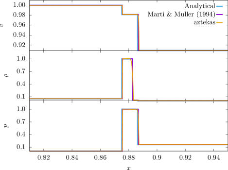
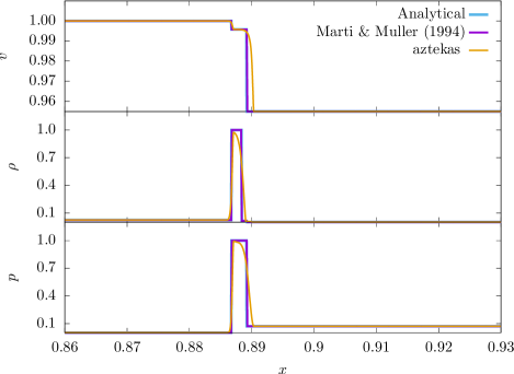
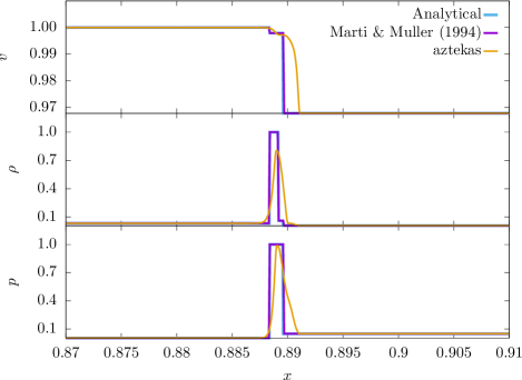
Figure 4: Snapshot at time $t=0.39$ for the hydrodynamical quantities of a working surface that moves to the right. From top to bottom the plots present pressure $p$, mass density $\rho$ and velocity $v$ profiles as a function of position. Continuous blue and purple lines represent the analytical (this article) and semi-analytic (Marti & Muller, 1994) solutions respectively (both merge together). Orange lines represent a 1DRHD numerical simulation using the aztekas code (http://aztekas.org ©2008 Sergio Mendoza & Daniel Olvera and ©2018 Alejandro Aguayo-Ortiz & Sergio Mendoza). Horizontal lines represent the spatial position of the two shock waves. The horizontal axis scale was chosen in such a way that the initial discontinuity at time $t=0$ occured at $x=0.5$ on a “numerical box” for which $0\leq x\leq 1$. The vertical axis was chosen in such a way that the particular hydrodynamical quantity is normalised to its maximum value for each particular panel. The analytic solution presented in this article and the semi-analytic one of Marti & Muller (1994) are almost identical to one another.

Case	$\delta\rho$	$\delta p$	$\delta v$	$\delta(\Gamma v)$
(a)	$\lesssim 2.7\times 10^{-3}$	$\lesssim 1.6\times 10^{-5}$	$\lesssim 2.6\times 10^{-4}$	$\lesssim 6.9\times 10^{-3}$
(b)	$\lesssim 5.8\times 10^{-4}$	$\lesssim 6.1\times 10^{-7}$	$\lesssim 6.8\times 10^{-6}$	$\lesssim 8.1\times 10^{-4}$
(c)	$\lesssim 1.0\times 10^{-3}$	$\lesssim 6.5\times 10^{-7}$	$\lesssim 2.0\times 10^{-8}$	$\lesssim 4.8\times 10^{-6}$

Table 2: The Table shows the maximum relative error $\delta X:=|X_{\text{M}}-X|/X_{\text{M}}$, where X stands for mass density $\rho$, pressure $p$, velocity $v$ and the product $\Gamma v$. The subindex M refers to the semi-analytical solution of Marti & Muller (1994). Quantities without subindex are our full ultra-relativistic analytical solution. Cases (a), (b) and (c) refer to the numerical simulations performed in Figure 4. We also compared our results with much greater initial pressures, densities and velocities as the ones corresponding to those cases, reaching Lorentz factors $\sim 700$ obtaining $\delta\rho\lesssim 3.6\times 10^{-4}$, $\delta p\lesssim 4.6\times 10^{-7}$ and $\delta v\lesssim 8.1\times 10^{-6}$.

6 Energy inside the working surface

The total energy $E(t)$ inside the working surface, i.e. between both shocks, is an important quantity to take into account for astrophysical processes, since the gas inside it has been heated through two strong shock waves and it is expected to cool via some efficient radiation process. To take into account this full radiation process is outside the scope of the present article. However, we can make a few assumptions in order to have a first glance as to the relevance of such an important process that occurs inside relativistic astrophysical jets. In what follows we assume that the total energy $E(t)$ is radiated away completely from the working surface due to some very efficient cooling process and so, it is possible to calculate the energy loss or the luminosity $L(t)$ by computing the negative power $-\mathrm{d}E/\mathrm{d}t$ emitted by the working surface. This assumption is a first approximation to the problem since a fluid particle crossing any of the shock waves and radiating all its energy ceases to have physical meaning, and will be sufficient for the first glance approximation we are dealing with. We also assume that at a certain time $t$ the energy density between the left shock wave $S_{1}$ and the tangential discontinuity $T$ is only given by $e_{3}(t)$, and that between the tangential discontinuity $T$ and the right shock wave $S_{1}$ is given by $e_{3^{\prime}}(t)$. This is a simple approximation since formally both energy densities $e_{3}$ and $e_{3^{\prime}}$ are functions of the position $z$ along the injected direction of the flow and time $t$. Nevertheless, since our first assumption is that the total energy within the working surface is fully radiated away, this statement constitutes a first good approximation.

6.1 Periodic velocity.

In order to show how to compute the emitted power by the working surface for a simple model, let us assume that the flow injection is periodic following the assumptions of Mendoza et al. (2009), with a periodic injected velocity given by:

$$v_{1}=v_{10}+v_{11}\sin(\omega t),$$ (34)

with $v_{2}=\text{const.}$, together with a constant background injected velocity $v_{10}$ close to the speed of light. The small positive parameter $v_{11}\ll 1$ and $\omega$ is the angular frequency of the oscillating flow. This choice produces a small sinusoidal perturbation about a background velocity $v_{10}$ close to the speed of light. The parameter $v_{11}\sin(\omega t)$ is chosen small enough so that the motion of the flow is always subluminal. Note that since the maximum value for the velocity is obtained when $\sin(\omega t=1)$, then a subluminal velocity $v_{1}$ at that maximum value is such that $1-v_{1}|_{\text{max}}=1-v_{10}-v_{11}>0$, so that $v_{11}/\left(1-v_{10}\right)<1$. In other words, the Lorentz factor associated to the velocity $v_{1}$ is given by:

$$\Gamma_{1}=\frac{1}{\sqrt{2\left(1-v_{10}\right)}}\left\{1-\frac{v_{11}}{2\left(1-v_{10}\right)}\sin(\omega t)\right\}.$$ (35)

The total energy $E$ inside the working surface, i.e. between both shock waves, is given by the volume $V$ integral:

$$E=\int_{V_{1}}e_{3}\,\mathrm{d}V+\int_{V_{2}}e_{3^{\prime}}\,\mathrm{d}V.$$ (36)

In the previous equation, the volume $V_{1}$ represents the volume between the left shock wave $S_{1}$ and the contact discontinuity $T$ with a transverse area $A$. The volume $V_{2}$ is taken from the tangential discontinuity $T$ to the right shock wave $S_{2}$ with the same transverse area $A$. Since the flow has plannar symmetry, equation (36) can be simplified as:

$$E=A\int_{S_{1}}^{T}e_{3}\,\mathrm{d}z+A\int_{T}^{S_{2}}e_{3^{\prime}}\,\mathrm{d}V=A\int_{S_{1}}^{S_{2}}e_{3}\mathrm{d}z.$$ (37)

The last step in the previous equation follows from the fact that $e_{3}=e_{3^{\prime}}$. In what follows and for the purpose of the current calculation, we set the transverse area $A=1$ and since in our model $e_{3}=e_{3}(t)$ only as stated above, the previous equation means that:

$$E=e_{3}\,\Delta z,$$ (38)

where $\Delta z$ is the distance between both shock waves. To compute this length, we substitute equation (35) into equations (31) and (32) to obtain a differential equation for the positions $z_{1}$ and $z_{2}$ of the left and right shock waves respectively:

$$\frac{\mathrm{d}z_{1}}{\mathrm{d}t}=v_{s1}=1-\frac{\sqrt{2\left(1-v_{10}\right)}}{\Gamma_{2}}\sqrt{\frac{p_{2}}{p_{1}}}\left\{1+\frac{v_{11}\sin(\omega t)}{2\left(1-v_{10}\right)}\right\},$$ (39)

$$\frac{\mathrm{d}z_{2}}{\mathrm{d}t}=v_{s1}=1-\frac{\sqrt{2\left(1-v_{10}\right)}}{4\Gamma_{2}}\sqrt{\frac{p_{2}}{p_{1}}}\left\{1+\frac{v_{11}\sin(\omega t)}{2\left(1-v_{10}\right)}\right\},$$ (40)

so that:

$$z_{1}=t-\frac{\sqrt{2\left(1-v_{10}\right)}}{\Gamma_{2}}\sqrt{\frac{p_{2}}{p_{1}}}\left\{t-\frac{v_{11}\cos(\omega t)}{2\omega\left(1-v_{10}\right)}\right\}+z_{1\text{init}},$$ (41)

$$z_{2}=t-\frac{\sqrt{2\left(1-v_{10}\right)}}{4\Gamma_{2}}\sqrt{\frac{p_{2}}{p_{1}}}\left\{t+\frac{v_{11}\cos(\omega t)}{2\omega\left(1-v_{10}\right)}\right\}+z_{2\text{init}},$$ (42)

where $z_{1\text{init}}$ and $z_{2\text{init}}$ are the initial poistions of the left and right shock waves respectively. With all the above relations and assuming a constant mass density and pressure discharges, the power loss inside the working surface is then given by:

$$\begin{split}L(t)&=-\eta\,\frac{\mathrm{d}E}{\mathrm{d}t}=\eta\,\frac{\mathrm{d}\Delta z}{\mathrm{d}t}\,e_{3}+\eta\,\frac{\mathrm{d}e_{3}}{\mathrm{d}t}\,\Delta z,\\ &=-3\eta\sqrt{2}\,P_{2}\sqrt{1-v_{10}}\left\{1+\frac{v_{11}\sin(\omega t)}{2\left(1-v_{10}\right)}\right\}-8\eta\omega v_{11}\,\times\\ &\left(\frac{\Gamma_{1}^{2}(t)}{\Gamma_{2}}\right)^{2}\sqrt{p_{1}p_{2}}\left\{\frac{3\left(1-v_{10}\right)}{2\sqrt{2}\,\Gamma_{2}}\sqrt{\frac{p_{2}}{p_{1}}}\left(t-\frac{\cos(\omega t)}{2\omega\left(1-v_{10}\right)}\right)+\right.\\ &\Delta z_{\text{init}}\bigg{\}},\end{split}$$ (43)

where $\Delta z_{\text{init}}$ is the initial length separation of both shock waves exactly at the time the working surface is formed and $\eta$ is an efficiency conversion factor from thermal energy power $-\mathrm{d}{E}/\mathrm{d}{t}$ to luminosity $L(t)$, such that $0<\eta\leq 1$. Figure 5 shows different power light curves obtained using this last result for various hydrodynamical parameters, chosen in such a way as to see the relevance of a high initial discontinuity between the pressures $p_{1}$ and $p_{2}$.

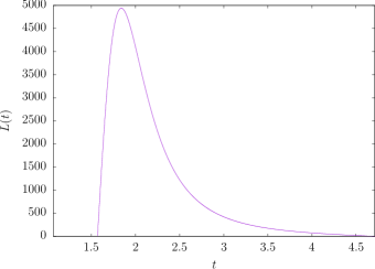
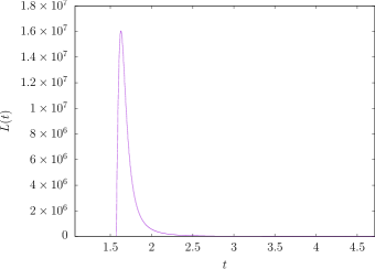
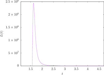
Figure 5: The figure shows three plots of the dissipated energy density inside a working surface From top to bottom the plots were produced with the following initial conditions: (1) $v_{10}=0.999$, $v_{11}=0.0009$, $p_{1}=30000.0$, $p_{2}=1000.0$, $v_{2}=0.1$; (2) $v_{10}=0.999998$, $v_{11}=0.00000199$, $p_{1}=40000.0$, $p_{2}=1000.0$, $v_{2}=0.96$; (3) $v_{10}=0.9999998$, $v_{11}=0.000000199$, $p_{1}=100000.0$, $p_{2}=90000.0$, $v_{2}=0.99$. In all plots we set $\omega=1$, $\Delta z_{\text{init}}=1$ and chose a system of units where the velocity is measured in units of the speed of light. The luminosity function $L(t)$ has been normalised to the background injected mechanical power $Ap_{1}v_{10}$, for a transverse area $A=1$, and to the efficiency conversion factor $\eta$.

7 Discussion

In this work we have found ultra-relativistic analytical solutions for a 1D planar working surface (two shock waves separating from a contact discontinuity) expanding into a moving medium. The equation of state of the flows outside and inside the working surface was also assumed to be ultra-relativistic, i.e. with the internal energy density being much greater than the rest mass internal energy density, and with a polytropic index $\kappa=4/3$ valid for ultra-relativistic gases. In general terms, this solution constitutes an analytical solution of the ultra-relativistic shock tube problem when e.g. fast flow reaches slower one in a 1D planar setup.

This type of solution can be well adapted to the blobs and knots observed in relativistic jets in Active Galactic Nuclei (AGN), microquasars and long Gamma-Ray Bursts (lGRB). In other words, the knots or blobs observed in many of these astrophysical jets can be interpreted as working surfaces moving along the jet. In order to calculate the energy dissipated inside the working surface as a function of time, we computed the energy density loss (luminosity density) as a function of time for a very particular model in which an ultra-relativistic varying velocity flow with constant discharge is assumed to be injected at the base of the jet. The luminosity density profiles produced by this efficient mechanism have similar shapes to the ones observed on the light curves of outbursts in AGN, microquasars and the prompt emission of lGBR. It is our intention in future works to use this model in order to understand and interpret in detail the light curves of many of these astrophysical jets using the methods of Mendoza et al. (2009); Cabrera et al. (2013); Coronado & Mendoza (2015); Coronado et al. (2016), but now with the full hydrodynamical solution presented in this article.

Data Availability

The data underlying this article are available in the article and in its online supplementary material.

Appendix A Lorentz factor relations for ultra-relativistic velocities

In this section, we show how to obtain a set of useful formulae in which Lorentz factors in different frames of reference are shown to be related to one another for the cases in which the velocities they refer to are highly relativistic.

Theorem 1

If $v_{1}$ and $v_{2}$ are two completely arbitrary velocities in units of the speed of light that satisfy the rule of velocity addition

$$v_{2}\mathbin{\mathchoice{\leavevmode\hbox to7.4pt{\vbox to7.4pt{\text{[drawing]}}}}{\leavevmode\hbox to7.4pt{\vbox to7.4pt{\text{[drawing]}}}}{\leavevmode\hbox to5.56pt{\vbox to5.56pt{\text{[drawing]}}}}{\leavevmode\hbox to4.21pt{\vbox to4.21pt{\text{[drawing]}}}}}v_{1}=\frac{v_{2}\pm v_{1}}{1\pm v_{2}v_{1}}, \pm \pm$$ (44)

then, the Lorentz factor associated with this transformation is:

$$\Gamma^{2}_{v_{2}\mathbin{\mathchoice{\leavevmode\hbox to7.33pt{\vbox to7.33pt{\text{[drawing]}}}}{\leavevmode\hbox to7.33pt{\vbox to7.33pt{\text{[drawing]}}}}{\leavevmode\hbox to5.49pt{\vbox to5.49pt{\text{[drawing]}}}}{\leavevmode\hbox to4.17pt{\vbox to4.17pt{\text{[drawing]}}}}}v_{1}}=\Gamma_{1}^{2}\Gamma_{2}^{2}(1\pm v_{2}v_{1})^{2}. \scriptstyle\pm \scriptstyle\pm$$ (45)

To demonstrate this property note that:

$$\begin{split}\Gamma^{2}_{v_{2}\mathbin{\mathchoice{\leavevmode\hbox to7.33pt{\vbox to7.33pt{\text{[drawing]}}}}{\leavevmode\hbox to7.33pt{\vbox to7.33pt{\text{[drawing]}}}}{\leavevmode\hbox to5.49pt{\vbox to5.49pt{\text{[drawing]}}}}{\leavevmode\hbox to4.17pt{\vbox to4.17pt{\text{[drawing]}}}}}v_{1}}&=\frac{1}{1-\left(\frac{v_{2}\pm v_{1}}{1\pm v_{2}v_{1}}\right)^{2}}=\frac{(1\pm v_{2}v_{1})^{2}}{(1\pm v_{2}v_{1})^{2}-(v_{2}\pm v_{1})^{2}},\\ &=\frac{(1\pm v_{2}v_{1})^{2}}{1+v_{2}^{2}v_{1}^{2}-v_{2}^{2}-v_{1}^{2}}=\frac{(1\pm v_{2}v_{1})^{2}}{(1-v_{1}^{2})(1-v_{2}^{2})}.\end{split} \scriptstyle\pm$$

Using relation (45), the following important properties of the Lorentz factors can be obtained:

Theorem 2

If $\Gamma_{1}\gg 1$ and $\Gamma_{2}\gg 1$, that is, $v_{1,2}=1-\varepsilon_{1,2}$, with $\varepsilon_{1,2}\ll 1$ sufficiently small quantities that make the velocities $v_{1}$ and $v_{2}$ to be ultra-relativistic, then

$$\Gamma_{1,2}=\frac{1}{\sqrt{2\,\varepsilon_{1,2}}},$$ (46)

which combined with relation (45) yields:

$$\Gamma_{v_{2}\oplus v_{1}} =2\Gamma_{1}\Gamma_{2}-\frac{1}{2}\left(\frac{\Gamma_{2}}{\Gamma_{1}}+\frac{\Gamma_{1}}{\Gamma_{2}}\right),$$

$$\Gamma_{v_{2}\ominus v_{1}} =\frac{1}{2}\left(\frac{\Gamma_{2}}{\Gamma_{1}}+\frac{\Gamma_{1}}{\Gamma_{2}}\right).$$ (47)

To proove this Theorem note first that equation (46) follows directly from the required assumptions. The set (47) can be obtained from taking the square root of equation (45):

$$\begin{split}\Gamma_{v_{2}\mathbin{\mathchoice{\leavevmode\hbox to7.33pt{\vbox to7.33pt{\text{[drawing]}}}}{\leavevmode\hbox to7.33pt{\vbox to7.33pt{\text{[drawing]}}}}{\leavevmode\hbox to5.49pt{\vbox to5.49pt{\text{[drawing]}}}}{\leavevmode\hbox to4.17pt{\vbox to4.17pt{\text{[drawing]}}}}}v_{1}}&=\Gamma_{1}\Gamma_{2}\left(1\pm(1-\varepsilon_{1})(1-\varepsilon_{2})\right),\\ &=\Gamma_{1}\Gamma_{2}\left(1\pm 1\mp(\varepsilon_{1}+\varepsilon_{2})\pm\varepsilon_{1}\varepsilon_{2}\right),\\ &=\Gamma_{1}\Gamma_{2}\begin{cases}2-(\varepsilon_{1}+\varepsilon_{2})+\varepsilon_{1}\varepsilon_{2},&\text{+ sign},\\ \varepsilon_{1}+\varepsilon_{2}-\varepsilon_{1}\varepsilon_{2},&\text{- sign},\end{cases}\\ &=\Gamma_{1}\Gamma_{2}\begin{cases}2-\frac{1}{2}(\Gamma_{1}^{-2}+\Gamma_{2}^{-2})+\frac{1}{4}\Gamma_{1}^{-2}\Gamma_{2}^{-2},&\text{+ sign},\\ \frac{1}{2}(\Gamma_{1}^{-2}+\Gamma_{2}^{-2})-\frac{1}{4}\Gamma_{1}^{-2}\Gamma_{2}^{-2},&\text{- sign},\end{cases}\\ &=\begin{cases}2\Gamma_{1}\Gamma_{2}-\frac{1}{2}\left(\frac{\Gamma_{2}}{\Gamma_{1}}+\frac{\Gamma_{1}}{\Gamma_{2}}\right),&\text{+ sign, to $\mathcal{O}(\Gamma^{-4})$},\\ \frac{1}{2}\left(\frac{\Gamma_{2}}{\Gamma_{1}}+\frac{\Gamma_{1}}{\Gamma_{2}}\right),&\text{- sign, to $\mathcal{O}(\Gamma^{-4})$}.\end{cases}\end{split} \scriptstyle\pm$$

As a direct consequence, it is found that:

Corollary 1

The sum of the Lorentz factors of (47) satisfy:

$$\Gamma_{v_{2}\oplus v_{1}}+\Gamma_{v_{2}\ominus v_{1}}=2\Gamma_{1}\Gamma_{2}.$$ (48)

To compute the square of relations (47), note that according to equation (45):

$$\begin{split}\Gamma^{2}_{v_{2}\mathbin{\mathchoice{\leavevmode\hbox to7.33pt{\vbox to7.33pt{\text{[drawing]}}}}{\leavevmode\hbox to7.33pt{\vbox to7.33pt{\text{[drawing]}}}}{\leavevmode\hbox to5.49pt{\vbox to5.49pt{\text{[drawing]}}}}{\leavevmode\hbox to4.17pt{\vbox to4.17pt{\text{[drawing]}}}}}v_{1}}&=\Gamma_{1}^{2}\Gamma_{2}^{2}(1\pm v_{2}v_{1})^{2},\\ &=\Gamma_{1}^{2}\Gamma_{2}^{2}\begin{cases}(2-\varepsilon_{1}+\varepsilon_{2})^{2},&\text{+ sign },\\ (\varepsilon_{1}+\varepsilon_{2})^{2},&\text{- sign },\end{cases}\\ &\approx\Gamma_{1}^{2}\Gamma_{2}^{2}\begin{cases}4(1-(\varepsilon_{1}+\varepsilon_{2})),&\text{+ sign},\\ \varepsilon_{1}^{2}+\varepsilon_{2}^{2}+2\varepsilon_{1}\varepsilon_{2},&\text{-sign },\end{cases}\\ &\approx\Gamma_{1}^{2}\Gamma_{2}^{2}\begin{cases}4(1-(\Gamma_{1}^{-2}+\Gamma_{2}^{-2}),&\text{+ sign},\\ \frac{1}{4}(\Gamma_{1}^{-4}+\Gamma_{2}^{-4})+\frac{1}{2}\Gamma_{1}^{-2}\Gamma_{2}^{-2},&\text{- sign},\end{cases}\\ &\approx\begin{cases}4\Gamma_{1}^{2}\Gamma_{2}^{2},&\text{+ sign},\\ \frac{1}{4}\left(\frac{\Gamma_{2}^{2}}{\Gamma_{1}^{2}}+\frac{\Gamma_{1}^{2}}{\Gamma_{2}^{2}}\right)+\frac{1}{2},&\text{- sign},\end{cases}\end{split} \scriptstyle\pm$$

and so:

Theorem 3

By the same assumptions of Theorem 2 it follows that:

$$\Gamma^{2}_{v_{2}\oplus v_{1}} =4\Gamma_{1}^{2}\Gamma_{2}^{2},$$ (49)

$$\Gamma^{2}_{v_{2}\ominus v_{1}} =\frac{1}{2}+\frac{1}{4}\left(\frac{\Gamma_{2}^{2}}{\Gamma_{1}^{2}}+\frac{\Gamma_{1}^{2}}{\Gamma_{2}^{2}}\right).$$ (50)

To conclude this section, consider that one of the two velocities in (45) has any arbitrary value, not necessarily ultra-relativistic. In such a case the following Theorem is satisfied:

Theorem 4

If $\Gamma_{1}\gg 1$ (i.e. when $v_{1}=1-1/{2\Gamma_{1}^{2}}$) then:

$$\Gamma^{2}_{v_{1}\mathbin{\mathchoice{\leavevmode\hbox to7.33pt{\vbox to7.33pt{\text{[drawing]}}}}{\leavevmode\hbox to7.33pt{\vbox to7.33pt{\text{[drawing]}}}}{\leavevmode\hbox to5.49pt{\vbox to5.49pt{\text{[drawing]}}}}{\leavevmode\hbox to4.17pt{\vbox to4.17pt{\text{[drawing]}}}}}v_{2}}=\Gamma_{1}^{2}\Gamma_{2}^{2}(1\pm v_{2})^{2}\ \text{for}\ \Gamma_{1}\gg 1, \scriptstyle\pm \scriptstyle\pm$$ (51)

for any value $v_{2}<1$.

To proove this theorem note that:

$$\begin{split}\Gamma^{2}_{v_{1}\mathbin{\mathchoice{\leavevmode\hbox to7.33pt{\vbox to7.33pt{\text{[drawing]}}}}{\leavevmode\hbox to7.33pt{\vbox to7.33pt{\text{[drawing]}}}}{\leavevmode\hbox to5.49pt{\vbox to5.49pt{\text{[drawing]}}}}{\leavevmode\hbox to4.17pt{\vbox to4.17pt{\text{[drawing]}}}}}v_{2}}&=\Gamma_{1}^{2}\Gamma_{2}^{2}(1\pm v_{1}v_{2})^{2},\\ &=\Gamma_{1}^{2}\Gamma_{2}^{2}\left(1\pm v_{2}\left[1-\frac{1}{2\Gamma_{1}^{2}}\right]\right)^{2},\\ &=\Gamma_{1}^{2}\Gamma_{2}^{2}\left(1\pm v_{2}\mp\frac{v_{2}}{2\Gamma_{1}^{2}}\right)^{2},\\ &=\Gamma_{1}^{2}\Gamma_{2}^{2}\left((1\pm v_{2})^{2}\mp\frac{(1\pm v_{2})v_{2}}{\Gamma_{1}^{2}}+...\right).\end{split} \scriptstyle\pm$$

References

• Aguayo-Ortiz et al. (2018) Aguayo-Ortiz A., Mendoza S., Olvera D., 2018, PLoS ONE, 13, e0195494
• Beloborodov & Uhm (2006) Beloborodov A. M., Uhm Z. L., 2006, ApJ, 651, L1
• Blandford & McKee (1976) Blandford R. D., McKee C. F., 1976, Physics of Fluids, 19, 1130
• Bondi (1964) Bondi H., 1964, Proceedings of the Royal Society of London Series A, 281, 39
• Cabrera et al. (2013) Cabrera J. I., Coronado Y., Benítez E., Mendoza S., Hiriart D., Sorcia M., 2013, MNRAS, 434, L6
• Coronado & Mendoza (2015) Coronado Y., Mendoza S., 2015, Ap&SS, 360, 1
• Coronado et al. (2016) Coronado Y., López-Corona O., Mendoza S., 2016, MNRAS, 462, 468
• Ghisellini et al. (2017) Ghisellini G., Righi C., Costamante L., Tavecchio F., 2017, MNRAS, 469, 255
• Hidalgo & Mendoza (2005) Hidalgo J. C., Mendoza S., 2005, Physics of Fluids, 17, 096101
• Katz (1994) Katz J. I., 1994, ApJ, 422, 248
• Kulkarni et al. (1999) Kulkarni S. R., et al., 1999, Nature, 398, 389
• Landau & Lifshitz (2013a) Landau L., Lifshitz E., 2013a, Statistical Physics: Course of Theoretical Physics. No. Vol. 5, Elsevier Science, https://books.google.com.mx/books?id=VzgJN-XPTRsC
• Landau & Lifshitz (2013b) Landau L., Lifshitz E., 2013b, Fluid Mechanics: Course of Theoretical Physics. No. Vol. 6, Elsevier Science, https://books.google.com.mx/books?id=eOBbAwAAQBAJ
• Lora-Clavijo et al. (2013) Lora-Clavijo F. D., Cruz-Pérez J. P., Siddhartha Guzmán F., González J. A., 2013, Revista Mexicana de Física E, 59, 28
• Marti & Muller (1994) Marti J. M., Muller E., 1994, Journal of Fluid Mechanics, 258, 317
• McKee & Colgate (1973) McKee C. R., Colgate S. A., 1973, Astrophysical Journal, 181, 903
• Mendoza (2000) Mendoza S., 2000, PhD thesis, Cambridge, U.K., http://www.mendozza.org/sergio/phdthesis
• Mendoza & Longair (2001) Mendoza S., Longair M. S., 2001, MNRAS, 324, 149
• Mendoza & Longair (2002) Mendoza S., Longair M. S., 2002, MNRAS, 331, 323
• Mendoza et al. (2009) Mendoza S., Hidalgo J. C., Olvera D., Cabrera J. I., 2009, MNRAS, 395, 1403
• Mitchell & Pope (1963) Mitchell T. P., Pope D. L., 1963, Royal Society of London. Series A, Mathematical and Physical Sciences, 227, 24
• Piran (1994) Piran T., 1994, in Fishman G. J., ed., American Institute of Physics Conference Series Vol. 307, Gamma-Ray Bursts. p. 495, doi:10.1063/1.45856
• Piran (1999) Piran T., 1999, Phys. Rep., 314, 575
• Piran (2004) Piran T., 2004, Reviews of Modern Physics, 76, 1143
• Rees (1978) Rees M. J., 1978, MNRAS, 184, 61P
• Romero et al. (2011) Romero G. E., Sunyaev R. A., Belloni T., eds, 2011, Jets at All Scales (IAU S275) IAU Symposium Vol. 275
• Sari & Piran (1995) Sari R., Piran T., 1995, ApJ, 455, L143
• Taub (1948) Taub A. H., 1948, Physical Review, 74, 328
• Taub (1967) Taub A. H., 1967, in Relativity Theory and Astrophysics. Vol.1: Relativity and Cosmology. pp 170–+
• Tooper (1965) Tooper R. F., 1965, Astrophysical Journal, 142, 1541
• Uhm (2011) Uhm Z. L., 2011, ApJ, 733, 86