A Morphological Classification Model to Identify Unresolved PanSTARRS1 Sources II: Update to the PS1 Point Source Catalog

Abstract

We present an update to the PanSTARRS-1 Point Source Catalog (PS1 PSC), which provides morphological classifications of PS1 sources. The original PS1 PSC adopted stringent detection criteria that excluded hundreds of millions of PS1 sources from the PSC. Here, we adapt the supervised machine learning methods used to create the PS1 PSC and apply them to different photometric measurements that are more widely available, allowing us to add $\sim$144 million new classifications while expanding the the total number of sources in PS1 PSC by $\sim$10%. We find that the new methodology, which utilizes PS1 forced photometry, performs $\sim$6–8% worse than the original method. This slight degradation in performance is offset by the overall increase in the size of the catalog. The PS1 PSC is used by time-domain surveys to filter transient alert streams by removing candidates coincident with point sources that are likely to be Galactic in origin. The addition of $\sim$144 million new classifications to the PS1 PSC will improve the efficiency with which transients are discovered.

DRAFT

1 Introduction

The proliferation of wide-field time-domain surveys over the past $\sim$decade has led to the discovery of a bevy of novel extragalactic transients (e.g., Quimby et al., 2011; Gezari et al., 2012; Drout et al., 2014; Gal-Yam et al., 2014; Abbott et al., 2017; Prentice et al., 2018; IceCube Collaboration et al., 2018). While these wide-field surveys have been enabled by significant advances in detector technology, software has proven equally important (e.g., Masci et al., 2017, 2019; Smith et al., 2020; Jones et al., 2020) as many of these critical discoveries have been facilitated by the rapid identification and dissemination of new transient candidates in near real time (e.g., Patterson et al., 2019).

Reliable catalogs identifying stars and galaxies, or similarly unresolved and resolved sources, are an essential cog in the machinery necessary to identify extragalactic transients. On a nightly basis, time-domain surveys are inundated with transient candidates, the vast majority of which are considered “bogus” (e.g., Bloom et al., 2012). Despite sophisticated software capable of whittling down the number of likely transients by several orders of magnitude (e.g., Brink et al., 2013; Goldstein et al., 2015; Duev et al., 2019; Smith et al., 2020), the number of candidates still vastly outpaces the spectroscopic resources necessary to classify everything that varies (e.g., Kulkarni, 2020). The aforementioned star–galaxy catalogs therefore play an essential role in the search for transients by removing stellar-like objects that are likely to be Galactic in origin.

The PanSTARRS-1 Point Source Catalog (PS1 PSC; Tachibana & Miller, 2018), which provides probabilistic point-source like classifications for $\sim$1.5 billion sources detected by PanSTARRS-1 (PS1; Chambers et al., 2016), was designed precisely to filter such sources. This catalog has been deployed by the Zwicky Transient Facility (ZTF; Bellm et al., 2019) and other surveys (Smith et al., 2020; Möller et al., 2020) to identify likely extragalactic transients. The PS1 PSC has been demonstrated to be an important ingredient in the systematic search for extragalactic transients (e.g., Fremling et al., 2020; De et al., 2020).

A downside to the PS1 PSC is that it does not provide classifications for sources that are not “detected” in the PS1 StackObjectAttributes table (see §3 in Tachibana & Miller, 2018). Of the $\sim$3 billion unique sources in the PS1 StackObjectAttributes table, the vast majority of those missing from the PS1 PSC are either spurious or have an extremely low signal-to-noise ratio (S/N), such that the methods in Tachibana & Miller (2018) would not provide a reliable classification. Additional sources are missing from the PS1 PSC because there are multiple rows within the PS1 StackObjectAttributes table that have the same ObjID and $\mathtt{primaryDetection}=1$. By definition this should not happen, and therefore these sources were excluded. For PS1 sources that are not in the PS1 PSC, ZTF reports a probability score $=0.5$, i.e., an ambiguous classification, when cross-matching newly observed variables with the PS1 catalog (see A for additional details about which PS1 sources are used by ZTF).

Here, we present an update to the PS1 PSC by classifying $\sim$144 million sources that were previously “missing” from the catalog. These classifications are made using different photometric measurements from the ones adopted in Tachibana & Miller (2018). While our new method performs slightly worse than the one in Tachibana & Miller (2018), we nevertheless achieve a similar level of accuracy with the new model. We apply our new model to the $\sim$426 million “missing” sources (classifying $\sim$34% of them), providing a new and useful supplement to the PS1 PSC.

Alongside this paper, we have released our open-source software needed to recreate the analysis in this study. These are available online at https://github.com/adamamiller/PS1_star_galaxy.

2 ML Model Data

2.1 PS1 Data

PS1 conducted a five filter ($g_{\mathrm{PS1}}$, $r_{\mathrm{PS1}}$, $i_{\mathrm{PS1}}$, $z_{\mathrm{PS1}}$, $y_{\mathrm{PS1}}$) time-domain survey covering $\sim$3/4 of the sky (Chambers et al., 2016). PS1 provides three different types of photometric measurements: there are mean flux measurements from the individual PS1 exposures of each field, there are stack flux measurements from the deeper stack images that co-add individual exposures, and there are forced-flux measurements that measure the flux in individual exposures at the location of all sources detected in the stack images. The mean photometry is limited by the depth of the individual exposures, while the stack photometry has a difficult to model point spread function (PSF) because images must be warped before they can be co-added. The forced-flux measurements provide an intermediate compromise as they are deeper than the mean flux measurements, while in principle having a more stable PSF than the stack images.

Tachibana & Miller (2018) show that the stack photometry works best when morphologically classifying resolved, extended sources and unresolved point sources. The methodology that we adopt here is extremely similar to Tachibana & Miller (2018), but we instead use PS1 forced photometry to classify sources that do not have suitable stack photometry. The forced-photometry-based model leads to slightly lower quality classifications (see §5).

2.2 ML Training Set

As a training set for the model, we use deep observations of the COSMOS field from the Hubble Space Telescope (HST). The superior resolution of HST enables reliable morphological classifications for sources as faint as $\sim$25 mag (Leauthaud et al., 2007). There are 80,867 bright HST sources from Leauthaud et al. (2007) that have PS1 counterparts (within a 1″match radius; see Tachibana & Miller, 2018) in the PS1 ForcedMeanObject table (see §3.1). Of those, the 47,825 PS1 sources with $\mathtt{nDetections}\geq 1$ are adopted as the training set for our model. This training set is $\sim$1.6% larger than the one used in Tachibana & Miller (2018) because more HST/COSMOS sources are “detected” in PS1 forced photometry.

3 ML Model Features

3.1 PS1 Forced Photometry Features

Regardless of the choice of algorithm, the basic goal of a machine learning model is to build a map between source features, numerical and/or categorical properties that can be measured for an individual source, and labels, the target output, often a classification, of the model. This mapping is learned via a training set, a subset of the data with known labels, after which the model can classify any source based on its features.

Tachibana & Miller (2018) introduced the concept of “white flux” features, whereby measurements in the five individual PS1 filters were summed, via a weighted mean, to produce a “total” flux or shape measurement across all filters. Machine learning models are limited by their training sets: there is no guarantee that their empirical mapping will correctly extend beyond the boundaries enclosed by the training set. Given the significant systematic uncertainties associated with Galactic reddening, and the tendency for spectroscopic samples, which are typically used to define training sets, to be biased in their target selection (see e.g., Miller et al., 2017), the motivation for “white flux” features becomes clear: they reduce potential biases in the final classifications due to selection effects in how the training set sources were targeted. Therefore, as in Tachibana & Miller (2018), we use “white flux” features in this study.

The PS1 StackObjectAttributes table provides both flux and shape (e.g., second moment of the radiation intensity) measurements in each of the five PS1 filters, whereas the PS1 ForcedMeanObject table only provides flux measurements.

To create the feature set for our machine learning model, we create “white flux” features for the six different flux measurements available in the ForcedMeanObject table (FPSFFlux, FKronFlux, FApFlux, FmeanflxR5, FmeanflxR6, FmeanflxR7), as well as the E1 and E2 measurements, which represent the mean polarization parameters from Kaiser et al. (1995). We use flux ratios, rather than the raw flux measurements, which provide morphological classifications that are independent of S/N (Lupton et al., 2001).

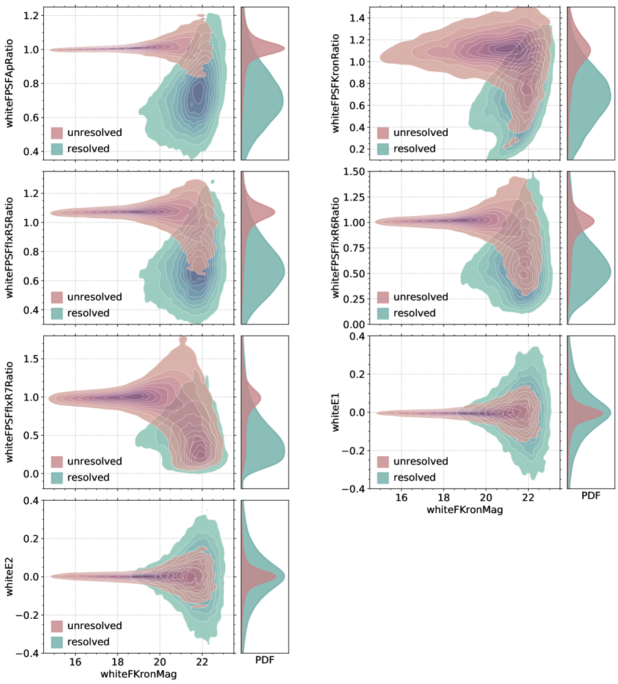
Figure 1: The primary square panels show Gaussian KDEs of the PDF for each of the “white flux” features as a function of whiteFKronMag ($=-2.5\log_{10}[\mathtt{whiteFKronFlux}/3631]$) for all sources in the training set. Unresolved point sources are shown via the red-purple contours, while resolved, extended objects are shown via blue-green contours. The shown contour levels extend from 0.9 to 0.1 in 0.1 intervals. To the right of each primary panel is a marginalized 1D KDE of the PDF for the individual features, where the amplitudes of the KDEs have been normalized by the relative number of point sources and extended objects.

Our final model includes nine features, five flux ratios:

$$\mathtt{whiteFPSFApRatio} =\frac{\mathtt{whiteFPSFlux}}{\mathtt{whiteFApFlux}},$$

$$\mathtt{whiteFPSFKronRatio} =\frac{\mathtt{whiteFPSFlux}}{\mathtt{whiteFKronFlux}},$$

$$\mathtt{whiteFPSFFmeanflxR5Ratio} =\frac{\mathtt{whiteFPSFlux}}{\mathtt{whiteFmeanflxR5Flux}},$$

$$\mathtt{whiteFPSFFmeanflxR6Ratio} =\frac{\mathtt{whiteFPSFlux}}{\mathtt{whiteFmeanflxR6Flux}},$$

$$\mathtt{whiteFPSFFmeanflxR7Ratio} =\frac{\mathtt{whiteFPSFlux}}{\mathtt{whiteFmeanflxR7Flux}},$$

the white polarization parameters: whiteE1 and whiteE2, and two “simple” distance measures: whiteFPSFKronDist and whiteFPSFKronDist (see §3.2). The distribution of these features for stars and galaxies in the training set is shown in Figures 1, 2, and 3.

Figure 1 shows that whiteFPSFApRatio is the most useful feature, aside from the “simple” features, to separate resolved and unresolved sources. This intuitively makes sense as PS1 ApFlux measurements are matched to the seeing, whereas the R5flx, R6flx, R7flx measurements use fixed aperture sizes. With multiple images taken under different observing conditions contributing to the final forced flux measurements, fixed aperture measurements should be more noisy.

3.2 The “Simple” Distance Features

Tachibana & Miller (2018) introduced a “simple” model to classify sources based solely on their measured whitePSFFlux and whiteKronFlux. The model was inspired by the use of flux ratios, which have been shown to provide a good discriminant between resolved and unresolved sources (e.g., the SDSS morphological CLASS parameter; Lupton et al., 2001). At moderate to low S/N, however, flux ratios no longer provide accurate classifications (see e.g., Figure 1). The simple model from Tachibana & Miller (2018) leverages this fact by measuring the distance of each source from a line drawn in the whitePSFFlux–whiteKronFlux plane. Unlike a flux ratio, the simple model preserves information about the S/N, meaning sources with large absolute distances from the dividing line can be classified with greater confidence.

Following from Equation 3 in Tachibana & Miller (2018), “simple” features can be calculated as:

$$\mathtt{whiteF1F2Dist}(a)=\frac{\mathtt{whiteF1}-a\times\mathtt{whiteF2}}{\sqrt{1+a^{2}}},$$ (1)

where whiteF1 and whiteF2 are the “white flux” measurements introduced in §3.1 (e.g., whiteFKronFlux), $a$ is the slope of the line in the whiteF1–whiteF2 plane, and whiteF1F2Dist is the orthogonal distance of a source from the line (sources above the line have positive values). For this study we construct two simple features for inclusion in our machine learning model: whiteFPSFFKronDist and whiteFPSFFApDist.

We determine the optimal value of $a$ for the simple features via cross validation. We find $a=0.7512$ for the whiteFPSFFKronDist feature and $a=0.7784$ for the whiteFPSFFApDist feature maximizes the FoM (see §4). Empirically whiteFPSFFApDist is better at separating resolved and unresolved sources than whiteFPSFFKronDist, and therefore the “simple” model, discussed below, is based on whiteFPSFFApDist. The whiteFPSFFApDist and whiteFPSFFKronDist distribution of resolved and unresolved sources is shown in Figures 2 and 3, respectively.

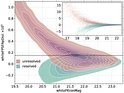
Figure 2: The distribution of $\mathtt{whiteFPSFKronDist}$ values for resolved, extended sources and unresolved point sources from the training set as a function of whiteKronMag. The colors and contours are the same as Figure 1. The horizontal dashed line shows the optimal threshold ($\mathtt{whiteFPSFKronDist}\geq 1.48\times 10^{-6}$) for resolved–unresolved classification. The upper-right inset shows a zoom-out highlighting the stark difference between stars and galaxies at the bright end.

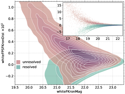
Figure 3: Same as Figure 2, but showing the distribution for whiteFPSFKronDist. A horizontal line is not shown as we do not recommend the use of only whiteFPSFKronDist for resolved-unresolved classification.

4 Training the ML Model

We construct a model to maximize the figure of merit (FoM) for our morphological classification model. Our aim is to retain nearly all the resolved, extended sources while excluding as many unresolved point sources as possible. Thus, our FoM is defined as the true positive rate (TPR) at a fixed false positive rate (FPR) = 0.005.

Using the nine features from §3, we use the random forest (RF) algorithm (Breiman, 2001), as implemented in scikit-learn (Pedregosa et al., 2011), to classify PS1 sources as resolved or unresolved. Briefly, the RF algorithm constructs an ensemble of decision trees (Breiman et al., 1984), where each tree is constructed using a bootstrapped sample of the training set (a method known as “bagging”; Breiman, 1996) and the split for each branch within the tree is selected from a random subset of the full feature set. The result is a lower variance estimator than is possible from a single decision tree.

To train the RF model, we replicate the procedure in Tachibana & Miller (2018). We use $k$-fold cross validation (CV) to optimize the model tuning parameters, namely the number of trees in the forest $N_{\mathrm{tree}}$, the random number of features for splitting at each node $m_{\mathrm{try}}$, and the minimum number of sources in a terminal leaf of the tree $\mathtt{nodesize}$. Our CV procedure utilizes both an inner and outer loop, each with $k=10$ folds. In the inner loop, a $k=10$ folds CV grid search is performed over the three tuning parameters, while predictions from the optimal grid location are applied to the 1/10 of the training set that was withheld in the outer loop. This process is then repeated for the remaining 9 folds in the outer loop. We adopt the average results from the 10 different grid searches to arrive at optimal model parameters of: $N_{\mathrm{tree}}=900$, $m_{\mathrm{try}}=3$, and $\mathtt{nodesize}=2$. The RF model results are not strongly dependent on the final choice of tuning parameters.

5 Results

5.1 Model Performance

Our aim is to maximize the FoM of the RF model. We show receiver operating characteristic (ROC) curves of the RF, simple, and PS1 models in Figure 4. From Figure 4, it is clear that the RF and simple models greatly outperform the PS1 model. Furthermore, while the gains are modest, the inclusion of all the “white flux” features and use of machine learning is justified as the RF model produces a higher FoM than the simple model.

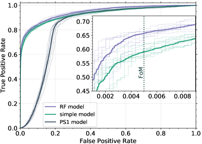
Figure 4: ROC curves comparing the relative performance of the PS1, simple, and RF models for HST sources with $i_{\mathrm{PS1}}$ detections. The thick slate gray, green, and purple lines show the ROC curves for the PS1, simple, and RF models, respectively. The light, thin lines show the ROC curves for the individual CV folds. The inset on the right shows a zoom in around FPR = 0.005, shown as a dotted vertical line, corresponding to the FoM (the PS1 model is not shown in the inset, because it has very low FoM).

The FoM of each of the three models is summarized in Table 1. In addition to providing the largest FoM, the RF model is also the most accurate and it has the largest area under the ROC curve (ROC AUC). We robustly conclude that, of the models considered here, the RF model is best. Comparing with Table 1 in Tachibana & Miller (2018), we find that the forced-photometry features derived in this study do not provide the same discriminating power as the PS1 stack-photometry features used in Tachibana & Miller (2018). Our new model performs $\sim$7% worse than the one in Tachibana & Miller (2018). In §6, we argue that this slight reduction in performance is more than offset by the $\sim$144 million additional sources that are now classified using the forced-photometry features.

Table 1: CV Results for the Training Set

model	FoM	Accuracy	ROC AUC
RF	0.657 $\pm$ 0.016	0.918 $\pm$ 0.003	0.945 $\pm$ 0.003
simple	0.591 $\pm$ 0.017	0.910 $\pm$ 0.007	0.930 $\pm$ 0.003
PS1	0.002 $\pm$ 0.001	0.764 $\pm$ 0.011	0.827 $\pm$ 0.009

Note. — Uncertainties represent the sample standard deviation for the 10 individual folds used in CV.

We show the CV accuracy of the RF, simple, and PS1 models as a function of whiteFKronMag in Figure 5. As in Tachibana & Miller (2018), we find that the RF model provides more accurate classifications than the alternatives.

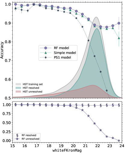
Figure 5: Top: Model accuracy as a function of whiteFKronMag for HST sources with $i_{\mathrm{PS1}}$ detections. Accuracy curves for the PS1, simple and RF models are shown as slate gray pentagons, green triangles, and purple circles, respectively. The bin widths are 0.5 mag, and the error bars represent the 68% interval from bootstrap resampling. Additionally, a Gaussian KDE of the PDF for the training set, as well as the unresolved point sources and resolved, extended objects in the same subset is shown in the shaded gray, red, and green regions, respectively. The amplitude of the star and galaxy PDFs have been normalized by their relative ratio compared to the full $i_{\mathrm{PS1}}$-band subset. Bottom: accuracy of resolved and unresolved classifications as a function of whiteFKronMag from the RF model (i.e., the TPR when treating each class as the positive class). Nearly all the resolved sources are correctly classified, because they dominate by number at low S/N (see text), while only bright unresolved sources are correctly classified.

The accuracy of each model shown in Figure 5 decreases for lower S/N sources. The accuracy curve for the RF and simple models feature a slight departure from expectation in that they do not decrease much from 22 to 24 mag. This quasi-plateau in the model accuracy can be understood as the result of two components of the training set: (i) unresolved sources completely dominate the source counts at these magnitudes, and (ii) the well-defined locus of unresolved sources in the training set (see Figure 1) becomes heavily blended with the resolved source population at these brightness levels. Taken together the model will be biased towards classifying all faint sources as resolved, despite the fact that we do not explicitly include flux measurements in the feature set. With 88.5% of the $\mathtt{whiteFKronMag}>22.5$ mag training set sources being unresolved, a quasi-plateau in accuracy of $\sim$88% makes sense. This is confirmed in the bottom panel of Figure 5, which shows the RF model true positive rate (TPR) for both resolved and unresolved sources as a function of whiteFKronMag. A near 100% TPR for faint resolved sources combined with a few correctly classified unresolved sources leads to the observed quasi-plateau in Figure 5.

5.2 The Updated PS1 PSC Catalog

With a new RF model in hand, we can now provide morphological classifications for the PS1 sources that are currently missing from the PS1 PSC. Of the $\sim$426 million “missing” sources, $\sim$144 million have PS1 DR2 ForcedMeanObject photometry that pass our detection criteria (see A for more details). A histogram showing the distribution of the RF classification score for these newly classified sources is shown in Figure 6.

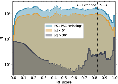
Figure 6: Histogram showing the RF classification scores for the $\sim$144 million newly classified sources from PS1. All of the newly classified sources are shown in blue, while Galactic plane sources ($|b|<5^{\circ}$) are shown in orange, and high galactic latitude sources ($|b|>30^{\circ}$) are shown in grey. The vertical dotted line shows the conservative classification threshold adopted in Tachibana & Miller (2018) (sources to the right of the line are considered point sources). The vast majority of the newly classified sources are in the Galactic plane.

Figure 6 shows that there are relatively few high-confidence classifications (i.e., very likely extended sources with RF score $\approx 0$ or very likely point sources with RF score $\approx 1$) among the “missing” sources. Figure 6 also reveals the likely explanation for this outcome: the vast majority of the newly classified sources are in the Galactic plane. Of the $\sim$144 million newly classified sources, $\sim$57% have galactic latitude $\lvert b\rvert<5$ deg, while $>95$% are in the Galactic plane ($\lvert b\rvert<15$ deg). The HST COSMOS field, from which we derive our training set, has $b\approx 42$ deg and as a result includes very few stellar blends, which are common at low galactic latitudes. The PS1 PSC also has significantly lower confidence classifications in the Galactic plane (see Figure 8 in Tachibana & Miller, 2018). That these sources were not “detected” in the PS1 stack images also suggests that it is difficult to make reliable photometric measurements using the PS1 data, which could also contribute to the lower confidence classifications. The upcoming third data release from the space-based Gaia telescope (Perryman et al., 2001) will improve this situation by classifying many of these ambiguous sources as stars via parallax and proper motion measurements.

Ultimately, this update to the PS1 PSC has identified 17,945,494 likely point sources using the optimized threshold from Tachibana & Miller (2018, RF score $\geq 0.83$). While this number is small compared to the $\sim$734 million point sources in the original PS1 PSC, these $\sim$18 million newly identified point sources would otherwise pass filters looking for extragalactic transients in the ZTF alert stream. Their removal will reduce the number of false positive transient candidates.

6 Deployment in the ZTF Real-Time Pipeline

The ZTF real-time pipeline (Masci et al., 2019) provides AVRO alert packets (see Patterson et al., 2019) containing information (e.g., flux, position, nearest neighbors) about any newly discovered sources of variability. The packets include morphological classifications, based on the PS1 PSC (Tachibana & Miller, 2018), for the three closest closed sources in the ZTF Stars table that are within 30″ of the newly observed variable source (see  A for a summary of the PS1 sources included in the ZTF Stars table). There are $\sim$426 million PS1 sources in the ZTF Stars table are not classified in the original PS1 PSC (see §5.2).

6.1 Updating RF Classifications with Gaia Stars

The Gaia Early Data Release 3 includes high-precision astrometric measurements collected over a 34 month timespan for $\sim$1.8 billion sources (Gaia Collaboration et al., 2020). Within ZTF, the PS1 PSC is primarily used to identify likely stars (i.e., point sources) and remove them from filters searching for extragalactic transients. To that end, we can supplement the RF classifications described in §5.2 with Gaia stars, which are identified via high-significance parallax and proper motion detections.

A common threshold for determining “high-significance” is $\mathrm{S/N}\geq 5$, which in the case of gaussian uncertainties corresponds to a $\sim$3$\times 10^{-7}$ probability that the observed signal is the result of noise. We can therefore select stars from Gaia sources with high S/N parallax or proper motion measurements. We adopt conservative significance thresholds because the formal uncertainties from Gaia are slightly underestimated (Fabricius et al., 2020) and because most of the “missing” sources in the ZTF Stars table are in the Galactic Plane (e.g., Figure 6). Fabricius et al. (2020) estimate that Gaia parallax measurements underestimate the uncertainties by a much as $\sim$60% in crowded regions. Similarly, proper motions are found to be underestimated by as much $\sim$80% in crowded regions (Fabricius et al., 2020). We therefore only consider Gaia sources with a parallax $\mathrm{S/N}\geq 8$ or a total proper motion $\mathrm{S/N}\geq 9$ to be stars.

Using the ESA Gaia archive we find there are 18,662,985 sources with either a high-significance parallax or proper motion detection in the ZTF Stars table that lack a classification in the original PS1 PSC. For these sources (11,479,512 of which have RF scores from §5.2) we update their scores to 1 in the ZTF Stars table. This effectively excludes each of these sources from filters designed to find extragalactic transients in the ZTF alert stream.

6.2 Practical Implementation of the Updated Catalog

Moving forward, ZTF alert packets now include $\sim$152 million additional classifications ($\sim$133.6 million RF classifications from §5.2, and $\sim$18.6 million from §6.1. The addition of these new classifications to the ZTF AVRO packets should not affect existing alert-stream filters, as we describe below.

Table 2: TPR and FPR for TM18 Thresholds

Catalog	Threshold	0.829	0.724	0.597	0.397	0.224
TM18	TPR	0.734	0.792	0.843	0.0904	0.947
	FPR	0.005	0.01	0.02	0.05	0.1
This work	TPR	0.684${}^{+0.005}_{-0.005}$	0.730${}^{+0.004}_{-0.005}$	0.772${}^{+0.004}_{-0.004}$	0.833${}^{+0.004}_{-0.003}$	0.902${}^{+0.004}_{-0.004}$
	FPR	0.005${}^{+0.001}_{-0.000}$	0.009${}^{+0.001}_{-0.001}$	0.016${}^{+0.001}_{-0.001}$	0.041${}^{+0.002}_{-0.001}$	0.111${}^{+0.002}_{-0.003}$

Note. — The table reports the TPR and FPR for different classification thresholds given in Table 3 in Tachibana & Miller (2018). To estimate the TPR and FPR we perform 10-fold CV on the entire training set, but only include sources with $\mathtt{nDetections}\geq 3$ in the final TPR and FPR calculations. The first row (TM18) summarizes the results from Tachibana & Miller (2018), while the second row uses the RF model from this study. The reported uncertainties represent the central 90% interval from 100 bootstrap resamples of the training set.

While a one-to-one mapping of point-source classification scores cannot be made between Tachibana & Miller (2018) and this study, the similarity between the two methodologies leads to classifications that are highly similar. Table 2 summarizes the TPR and FPR for different classification thresholds using the model from Tachibana & Miller (2018) and the RF model created in this study. The PS1 stack photometry used in Tachibana & Miller (2018) consistently produces a higher TPR, by $\sim$6–8%, than the PS1 forced photometry. The PS1 forced photometry used in this study does have a lower FPR than Tachibana & Miller (2018) for all but the most liberal point-source classification cuts. Thus, applying classification cuts developed for the original PS1 PSC will ultimately lead to a higher TPR, as previously unclassified point sources can now be removed from the stream, without experiencing an overall increase in the FPR. As a result, we conclude that the vast majority of users will not experience any significant change in the results to their filters, aside from a slight reduction in false negatives (stars that are classified as galaxies), following the update to the ZTF Stars table.

7 Discussion

During the preparation of this manuscript, Beck et al. (2020) published the Pan-STARRS1 Source Types and Redshifts with Machine learning (PS1-STRM) catalog, which includes the machine learning classification of PS1 sources as either stars, galaxies, or quasars. Like this study, Beck et al. (2020) use PS1 forced photometry to provide classifications. There are a couple of differences between the catalogs: the PS1-STRM classifies all $\sim$2.9 billion sources in the PS1 ForcedMeanObject table, while the updated PS1 PSC only classifies $\sim$half that many sources. Another difference between the two catalogs is that the PS1-STRM uses a neural-network classifier, whereas the PS1 PSC uses the RF algorithm. Finally, the PS1-STRM uses full color information in their classifier whereas the PS1 PSC uses “white flux” features (see §3.1).

The most important distinction between the two catalogs, in our estimation, is their training sets. The PS1-STRM is trained using spectroscopic labels that predominantly come from the Sloan Digital Sky Survey (SDSS; Abolfathi et al., 2018), whereas the PS1 PSC is trained via morphological classifications from HST. An SDSS-based training set has two distinct advantages: it is nearly two orders of magnitude larger than the HST training set and it includes redshift information (which can be used to estimate photometric redshifts, as is done in the PS1-STRM).

When considering only morphological classification, or similarly star-galaxy separation, an SDSS-based training set produces biased classifications (Miller et al., 2017; Tachibana & Miller, 2018). The SDSS spectroscopic targeting algorithm was biased towards specific source classes, such as luminous red galaxies, and as a result SDSS spectra are not representative of the average source in PS1 (see Figure 1 in Tachibana & Miller, 2018). Furthermore, the SDSS training set is distinctly biased towards point sources at the faint end ($r\gtrsim 21$ mag), which leads to models that overestimate the prevalence of point sources at these brightness levels (see e.g., Figure 7 in Tachibana & Miller, 2018). It is for these reasons that we adopt the HST training set for the PS1 PSC, despite its relatively modest size.

Ultimately, we recommend the use of both catalogs. Despite the different methodologies and training sets, we expect the classifications to largely be in agreement for bright sources ($r\lesssim 20$ mag). In cases where the catalogs agree, the classifications can be treated as extremely confident. Most of the disagreements will occur at the faint end, where both catalogs will provide noisier estimates. For faint sources where the catalogs disagree, users should consider applying an additional prior based on the observed source counts in the Universe (e.g., Henrion et al., 2011). At high galactic latitudes, nearly all the very faint sources are galaxies, while within the Galactic plane nearly everything will be a star.

8 Conclusions

We have presented an update to the PS1 PSC (Tachibana & Miller, 2018), by classifying $\sim$144 million sources that were previously “missing.” The new classifications are made using a new RF model that utilizes photometric and shape features from the PS1 DR2 ForcedMeanObject table.

The training set and methodology are nearly identical to those used in Tachibana & Miller (2018), with the major difference being that that study used features from the PS1 DR1 StackObjectAttributes table. The similarity in methodology is intentional, as it allows new classifications for the previously “missing” sources to be incorporated into the PS1 PSC without a need for significant revisions to existing filters that are applied to the ZTF alert stream. We find that the new model performs $\sim$6–8% worse than the one presented in Tachibana & Miller (2018, see Table 2). Nevertheless, the slight degradation in performance is more than offset by the addition of $>$144 million newly classified sources. The update to the PS1 PSC presented here will improve the extragalactic transient search efficiency for ZTF.

Spectroscopic observations from SDSS have now fueled the training sets for machine learning models to separate stars and galaxies for more than a decade (e.g., Ball et al., 2006; Beck et al., 2020). These labels have proven extremely valuable as they have been applied to several surveys beyond SDSS (e.g., Miller et al., 2017; Beck et al., 2020). Our ability to use methods built on empirical training sets is going to be severely limited by the Vera C. Rubin Observatory, whose images will be predominantly populated by extremely faint sources ($r\approx 24$ mag; Ivezić et al., 2019). With few spectroscopic classifications of any kind at these depths, the separation of stars and galaxies in Rubin Observatory data is going to largely rely on data from the Rubin Observatory itself. In this regime machine learning is unlikely to play a leading role, and purely photometric methods will be required to separate stars and galaxies (e.g., Slater et al., 2020) and triage the Rubin Observatory alert stream to remove stellar variables prior to the search for extragalactic transients.

Appendix A The ZTF–PS1 Morphological Catalog

The ZTF database contains a table (Stars) with sources selected from the PS1 DR1 that are used to provide morphological classifications in the ZTF alert packets. The ZTF Stars table was seeded from the PS1 MeanObject table and includes all PS1 MeanObject sources with $\mathtt{nDetections}\geq 3$. There are 1,919,106,844 sources in the ZTF Stars table. Of these, 1,484,281,394 are classified in the PS1 PSC and another 8,520,167 are classified as point sources based on Gaia parallax and/or proper motion measurements (Tachibana & Miller, 2018). Therefore, there are 426,305,283 sources in the ZTF Stars table that did not meet the quality cuts necessary to be included in the PS1 PSC.

For the $\sim$426 million ZTF Stars table sources not in the PS1 PSC, 5,885,633 had multiple rows in the PS1 StackObjectAttributes table with $\mathtt{primaryDetection}=1$, while the rest were not “detected” in the PS1 stacks. As described in §5.2, 144,870,754 of the previously “missing” sources pass our ForcedMeanObject “detection” criteria (see §2.2) and are now included in the PS1 PSC.

The remaining $\sim$281 million sources do not have reliable PS1 stack or forced photometry, and as a result remain in the ZTF Stars table with an ambiguous score of 0.5. About 8% of the still unclassified ZTF Stars table sources are not present in PS1 DR2 (mostly because they have declination $\delta<-30$ deg). Furthermore, $\sim$34% of these $\sim$281 million sources have $\mathtt{nDetections}=3$, and $\sim$55% have $\mathtt{nDetections}\leq 5$. That these sources have so few detections in PS1 increases the probability that they may be spurious, and even if they are not spurious, they are otherwise very low S/N detections, which do not produce highly confident classifications.

References

- Abbott et al. (2017) Abbott, B. P., Abbott, R., Abbott, T. D., et al. 2017, ApJ, 848, L12
- Abolfathi et al. (2018) Abolfathi, B., Aguado, D. S., Aguilar, G., et al. 2018, ApJS, 235, 42
- Astropy Collaboration et al. (2013) Astropy Collaboration, Robitaille, T. P., Tollerud, E. J., et al. 2013, A&A, 558, A33
- Astropy Collaboration et al. (2018) Astropy Collaboration, Price-Whelan, A. M., Sipőcz, B. M., et al. 2018, AJ, 156, 123
- Ball et al. (2006) Ball, N. M., Brunner, R. J., Myers, A. D., & Tcheng, D. 2006, ApJ, 650, 497
- Beck et al. (2020) Beck, R., Szapudi, I., Flewelling, H., et al. 2020, MNRAS
- Bellm et al. (2019) Bellm, E. C., Kulkarni, S. R., Graham, M. J., et al. 2019, PASP, 131, 018002
- Bloom et al. (2012) Bloom, J. S., Richards, J. W., Nugent, P. E., et al. 2012, PASP, 124, 1175
- Breiman (1996) Breiman, L. 1996, Machine Learning, 24, 123
- Breiman (2001) —. 2001, Machine Learning, 45, 5
- Breiman et al. (1984) Breiman, L., Friedman, J., Stone, C. J., & Olshen, R. A. 1984, Classification and regression trees (CRC press)
- Brink et al. (2013) Brink, H., Richards, J. W., Poznanski, D., et al. 2013, MNRAS, 435, 1047
- Chambers et al. (2016) Chambers, K. C., Magnier, E. A., Metcalfe, N., et al. 2016, ArXiv e-prints
- De et al. (2020) De, K., Kasliwal, M. M., Tzanidakis, A., et al. 2020, arXiv, arXiv:2004.09029
- Drout et al. (2014) Drout, M. R., Chornock, R., Soderberg, A. M., et al. 2014, ApJ, 794, 23
- Duev et al. (2019) Duev, D. A., Mahabal, A., Masci, F. J., et al. 2019, MNRAS, 489, 3582
- Fabricius et al. (2020) Fabricius, C., Luri, X., Arenou, F., et al. 2020, arXiv, arXiv:2012.06242
- Fremling et al. (2020) Fremling, C., Miller, A. A., Sharma, Y., et al. 2020, ApJ, 895, 32
- Gaia Collaboration et al. (2020) Gaia Collaboration, Brown, A. G. A., Vallenari, A., et al. 2020, arXiv, arXiv:2012.01533
- Gal-Yam et al. (2014) Gal-Yam, A., Arcavi, I., Ofek, E. O., et al. 2014, Nature, 509, 471
- Gezari et al. (2012) Gezari, S., Chornock, R., Rest, A., et al. 2012, Nature, 485, 217
- Goldstein et al. (2015) Goldstein, D. A., D’Andrea, C. B., Fischer, J. A., et al. 2015, AJ, 150, 82
- Henrion et al. (2011) Henrion, M., Mortlock, D. J., Hand, D. J., & Gandy, A. 2011, MNRAS, 412, 2286
- Hunter (2007) Hunter, J. D. 2007, Computing In Science & Engineering, 9, 90
- IceCube Collaboration et al. (2018) IceCube Collaboration, Aartsen, M. G., Ackermann, M., et al. 2018, Science, 361, eaat1378
- Ivezić et al. (2019) Ivezić, Ž., Kahn, S. M., Tyson, J. A., et al. 2019, ApJ, 873, 111
- Jones et al. (2020) Jones, D. O., Foley, R. J., Narayan, G., et al. 2020, arXiv, arXiv:2010.09724
- Kaiser et al. (1995) Kaiser, N., Squires, G., & Broadhurst, T. 1995, ApJ, 449, 460
- Kulkarni (2020) Kulkarni, S. R. 2020, arXiv, arXiv:2004.03511
- Leauthaud et al. (2007) Leauthaud, A., Massey, R., Kneib, J.-P., et al. 2007, ApJS, 172, 219
- Lupton et al. (2001) Lupton, R., Gunn, J. E., Ivezić, Z., et al. 2001, Astronomical Society of the Pacific Conference Series, 238, 269
- Masci et al. (2017) Masci, F. J., Laher, R. R., Rebbapragada, U. D., et al. 2017, PASP, 129, 014002
- Masci et al. (2019) Masci, F. J., Laher, R. R., Rusholme, B., et al. 2019, PASP, 131, 018003
- McKinney (2010) McKinney, W. 2010, 56
- Miller et al. (2017) Miller, A. A., Kulkarni, M. K., Cao, Y., et al. 2017, AJ, 153, 73
- Möller et al. (2020) Möller, A., Peloton, J., Ishida, E. E. O., et al. 2020, arXiv, arXiv:2009.10185
- Patterson et al. (2019) Patterson, M. T., Bellm, E. C., Rusholme, B., et al. 2019, PASP, 131, 018001
- Pedregosa et al. (2011) Pedregosa, F., Varoquaux, G., Gramfort, A., et al. 2011, Journal of Machine Learning Research, 12, 2825
- Perryman et al. (2001) Perryman, M. A. C., de Boer, K. S., Gilmore, G., et al. 2001, A&A, 369, 339
- Prentice et al. (2018) Prentice, S. J., Maguire, K., Smartt, S. J., et al. 2018, ApJ, 865, L3
- Quimby et al. (2011) Quimby, R. M., Kulkarni, S. R., Kasliwal, M. M., et al. 2011, Nature, 474, 487
- Slater et al. (2020) Slater, C. T., Ivezić, Ž., & Lupton, R. H. 2020, AJ, 159, 65
- Smith et al. (2020) Smith, K. W., Smartt, S. J., Young, D. R., et al. 2020, PASP, 132, 085002
- Tachibana & Miller (2018) Tachibana, Y., & Miller, A. A. 2018, PASP, 130, 128001
- Virtanen et al. (2020) Virtanen, P., Gommers, R., Oliphant, T. E., et al. 2020, Nature Methods, 17, 261