Machine learning prediction of critical transition and system collapse

Abstract

To predict a critical transition due to parameter drift without relying on model is an outstanding problem in nonlinear dynamics and applied fields. A closely related problem is to predict whether the system is already in or if the system will be in a transient state preceding its collapse. We develop a model free, machine learning based solution to both problems by exploiting reservoir computing to incorporate a parameter input channel. We demonstrate that, when the machine is trained in the normal functioning regime with a chaotic attractor (i.e., before the critical transition), the transition point can be predicted accurately. Remarkably, for a parameter drift through the critical point, the machine with the input parameter channel is able to predict not only that the system will be in a transient state, but also the average transient time before the final collapse.

In nonlinear and complex dynamical systems, a catastrophic collapse is often preceded by transient chaos. For example, in electrical power systems, voltage collapse can occur after the system enters into the state of transient chaos Dhamala and Lai (1999). In ecology, slow parameter drift caused by environmental deterioration can induce a transition into transient chaos, after which species extinction follows McCann and Yodzis (1994a); Hastings et al. (2018). A common route to transient chaos is a global bifurcation termed crisis Grebogi et al. (1983), at which a chaotic attractor collides with its own basin boundary, is destroyed and becomes a chaotic transient. In the real world, the accurate system equations are often unknown but only measured time series are available. Model-free and data driven prediction of the critical transition and system collapse in advance of their occurrences, while the system is currently operating in a normal regime with a chaotic attractor, has been an outstanding problem. If the underlying equations of the system have a simple mathematical structure, e.g., with the velocity field consisting of power series or Fourier series terms only, then sparse optimization methods such as compressive sensing can be exploited to identify the system equations Wang et al. (2011, 2016) and consequently to predict transitions. Here, we assume that our system does not meet this condition and set out to develop a machine learning framework to predict the critical transition.

A closely related problem is to determine if the system is already in a transient state - the question of “how do you know you are in a transient?”. In nonlinear dynamics, this is one of the most difficult questions because the underlying system can be in a long transient in which all measurable physical quantities exhibit essentially the same behaviors as if the system were still in a sustained state with a chaotic attractor. Applying the traditional method of delay coordinate embedding Takens (1981) to such a case would yield estimates of dynamical invariants such as the Lyapunov exponents and fractal dimensions, but it would give no indication that the system is already in a transient and so an eventual collapse is inevitable. Developing a model-free, purely data-driven predictive paradigm to address this problem is of considerable value to solving some of the most pressing problems in the modern time. Due to global warming and climate change, some natural systems may have already been in a transient state awaiting a catastrophic collapse to occur. A reliable determination at the present that the system has already passed the critical transition or a “tipping” point to a transient state would send a clear message to policy makers and the general public that actions must be taken immediately to avoid the otherwise inevitable catastrophic collapse.

In this Letter, we develop a machine learning framework to predict critical transition and transient chaos in nonlinear dynamical systems. We exploit reservoir computing, a class of recurrent neural networks Jaeger (2001); Mass et al. (2002); Jaeger and Haas (2004); Manjunath and Jaeger (2013), a research area that has gained considerable momentum as a powerful paradigm for model-free prediction of nonlinear and chaotic dynamical systems Haynes et al. (2015); Larger et al. (2017); Pathak et al. (2017); Lu et al. (2017); Duriez et al. (2017); Lu et al. (2018); Pathak et al. (2018a, b); Carroll (2018); Nakai and Saiki (2018); Roland and Parlitz (2018); Weng et al. (2019); Griffith et al. (2019); Jiang and Lai (2019); Vlachas et al. (2019); Fan et al. (2020). Our articulated reservoir computing structure differs from the conventional one in that we designate an additional input channel for the bifurcation parameter, as shown in Fig. 1(a). The basic idea of our framework is explained in Fig. 1(b), a schematic bifurcation diagram of a typical nonlinear system. In the green region, there is a chaotic attractor together with periodic windows, in which the system functioning is normal. A catastrophic bifurcation occurs at the critical parameter value defining the end of the green region, where the chaotic attractor is destroyed through a crisis transition. For a parameter value slightly beyond the critical point, there is transient chaos leading to collapse. Suppose that, currently, the system operates in the normal regime. Given a certain amount of parameter drift, the two goals are: (i) to predict the transition point so as to determine whether the system will be in a transient chaotic regime heading to collapse and (ii) if yes, on average how long the system could survive, i.e., to predict the average lifetime of the chaotic transient. Because time series data from multiple parameter values are needed, it is necessary to specify the parameter value at which the data are taken - a task that can be accomplished by inputting the parameter value to all nodes in the underlying neural network. We demonstrate that our proposed machine learning framework can accomplish the two goals with three examples: an electrical power system susceptible to voltage collapse through transient chaos Dhamala and Lai (1999), a three-species food chain model McCann and Yodzis (1994a) in ecology in which a catastrophic transition leads to transient chaos and then species extinction, and the Kuramoto-Sivashinsky system Kuramoto (1978); Sivashinsky (1980) in the regime of transient spatiotemporal chaos Hyman et al. (1986). We show that, training a reservoir network of reasonable size, e.g., 1000 nodes, with time series data taken from three parameter values in the normal chaotic regime, the machine is able to predict not only the collapse point but also transient chaos for parameter values beyond the critical point. A remarkable feature is that, after the critical transition, the probability distribution of the transient lifetime of the machine generated trajectories from an ensemble of initial conditions agrees with the true distribution, indicating that, for a given parameter drift into the transient chaos regime, the machine is able to predict, on average, how long the system can “survive” before collapse.

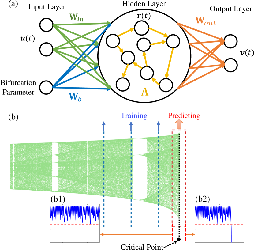
Figure 1: Modified reservoir computing scheme and illustration of the idea to predict critical transition and collapse. (a) Structure of the modified reservoir computing machine with an input parameter channel. The system consists of three layers: the input layer, the hidden layer and the output layer. Vectors $\mathbf{u}(t)$, $\mathbf{r}(t)$, and $\mathbf{v}(t)$ denote the set of input signals (measured time series from the dynamical variables of the target system), the dynamical state of the reservoir network (hidden layer), and the set of output signals representing the machine’s prediction. The bifurcation parameter is designated as an additional input. (b) The reservoir computing machine is trained with time series taken from a few parameter values in the green regime in which the system operates normally - indicated by the three vertical blue dashed lines. After training, prediction can be made either for parameter values before the critical point (still in the green regime) or after, where in the former, the machine will predict that the system is safe (b1) but, importantly, for the latter, the machine will predict that the system will eventually collapse after transient chaos (b2).

For simplicity, we consider a catastrophic transition caused by variations in a single parameter. (Situations of multiple parameters can be treated with multiple parameter channels.) As shown in Fig. 1(a), the input layer maps the low-dimensional time series data $\mathbf{u}(t)$ into the high-dimensional hidden state $\mathbf{r}(t)$ through a matrix $\mathcal{W}_{in}$, and the output layer maps $\mathbf{r}(t)$ back into low-dimensional time series $\mathbf{v}(t)$ through another matrix $\mathcal{W}_{out}$. The input parameter channel is connected to every node of the reservoir network via the matrix $\mathcal{W}_{b}$. The reservoir network adjacency matrix $\mathcal{A}$ transfers information from the hidden states $\mathbf{r}(t)$ at $t$ to the next time step $\mathbf{r}(t+\Delta t)$. The dynamical evolution of the reservoir computing machine is described by $\mathbf{r}(t+\Delta t)=(1-\alpha)\mathbf{r}(t)+\alpha\tanh{[\mathcal{A}\cdot\mathbf{r}(t)+\mathcal{W}_{in}\cdot\mathbf{u}(t)+k_{b}\mathcal{W}_{b}(\mathbf{b}+b_{0})]}$ and $\mathbf{v}(t)=\mathcal{W}_{out}\cdot\mathbf{r}(t)$, where $\alpha$ is the leakage parameter, $k_{b}$ and $b_{0}$ are two hyperparameters determining the input of the bifurcation parameter into the reservoir network. Training is administered to adjust the output matrix $\mathcal{W}_{out}$ to minimize the difference between $\mathbf{v}(t)$ and $\mathbf{u}(t+\Delta t)$, so that the reservoir can predict the evolution of the target system into the future with input of the dynamical variables from the past. The matrices $\mathcal{W}_{in}$, $\mathcal{W}_{b}$ and $\mathcal{A}$ are chosen a priori and fixed during the training and prediction phases for efficiency. (A more detailed description of the training and predicting processes is provided in Sec. I of Supplementary Information (SI) SI .) We train the reservoir machine using time series from a few distinct parameter values - all in the normal or safe regime where the system still possesses a chaotic attractor, as shown in Fig. 1(b). Because of the additional parameter input channel, the machine trained with data at different parameter values will gain the ability to “sense” the variation in the parameter and the associated changes in the time series data from different parameter values. Such a well trained machine is a high-dimensional representation of the original dynamical system. Finally, to predict with what parameter drift the system will exhibit transient chaos and then collapse, we simply input the parameter value of interest into the parameter input channel. Then, at each time step, we collect the one-step prediction from the output layer $\mathbf{v}(t)$ and feed it back to the input layer $\mathbf{u}(t+\Delta t)=\mathbf{v}(t)$. Now the reservoir machine in the predicting phase is a closed-loop dynamical system with one constant external drive - the bifurcation parameter of interest. The machine in the predicting phase will be able to predict the system collapse preceded by transient chaos for the input value of bifurcation parameter.

To achieve better performance, for each target system, we choose the seven key hyperparameters of the reservoir computing machine based on Bayesian optimization Griffith et al. (2019), which are the average degree and the spectral radius of the reservoir network, the scales of the input matrix $\mathcal{W}_{in}$, parameters $k_{b}$, $b_{0}$, and $\alpha$, as well as the regularization parameter used during the training of the output matrix $\mathcal{W}_{out}$. (A more detailed description of these hyperparameters and their optimization can be found in Secs. I and V of SI SI .)

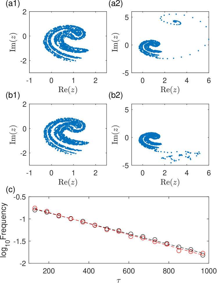
Figure 2: Predicting transient chaos and collapse of dynamics in a nonlinear optical cavity as described by the Ikeda map. (a1,a2) Typical behaviors of the system in the sustained and transient chaos regimes, respectively, for $\mu=0.99<\mu_{c}$ and $\mu=1.01>\mu_{c}$. (b1,b2) Predicted behaviors by the reservoir machine for the same values of $\mu$ as in (a1,a2), respectively. The machine predicts correctly the system collapse for $\mu>\mu_{c}$. (c) Actual (black) and predicted (red) exponential transient lifetime distributions for $\mu=\mu_{c}+0.02$.

To demonstrate that our machine learning approach represents a true advance in nonlinear systems prediction, we present two examples for which the sparse optimization methods fail. In particular, the basic requirement of any sparse optimization technique for finding the system equations is sparsity: when the system equations are expanded into a power series or a Fourier series, it must be that only a few terms are present so that the coefficient vectors to be determined from data are sparse Wang et al. (2011, 2016).

The first example is the Ikeda map Ikeda (1979); Ikeda et al. (1980); Hammel et al. (1985) that describes the dynamics of a laser pulse propagating in a nonlinear cavity: $z_{n+1}=\mu+\gamma z_{n}\exp{\left[i\kappa-i\eta/(1+|z_{n}|^{2})\right]}$, where $z$ is a complex dynamical variable and the bifurcation parameter $\mu$ is the dimensionless laser input amplitude (more details in Sec. IIA in SI SI ). When the map functions are expanded into a power series, all combinations of the powers of the dynamical variables are necessary. The coefficient vectors for the dynamical variables are absolutely dense, representing an extreme type of violation of the sparsity condition. The system exhibits a boundary crisis In et al. (1998) at $\mu_{c}=1.0027$ and the dynamical behaviors for $\mu<\mu_{c}$ and $\mu>\mu_{c}$ are shown in Figs. 2(a1) and  2((a2), respectively. There is a chaotic attractor for $\mu<\mu_{c}$, and transient chaos leading to an escape of the system out of the previous operation region for $\mu>\mu_{c}$. We train the reservoir machine at $\mu=0.91,0.94,0.97$ - all in the chaotic attractor regime. For each $\mu$ value, training is done such that the reservoir machine is able to predict the exact state evolution of the original system for several Lyapunov time. More importantly, we ensure that the predicted trajectories land on the chaotic attractor for an arbitrarily long stretch of time. After training, we apply some parameter change $\Delta\mu$ and test, for each resulting parameter value, whether the predicted system state is a chaotic attractor or a chaotic transient. An exemplary pair of the predicted state for $\mu<\mu_{c}$ and $\mu>\mu_{c}$ are shown in Figs. 2(b1) and 2(b2), respectively. It is remarkable that the reservoir machine is able to predict the collapse after a chaotic transient, as shown in Fig. 2(b2). Examining the prediction results for a set of systematically varied $\Delta\mu$ values enables determination of the critical bifurcation point, denoted as $\mu^{*}_{c}$. Averaging over 1,000 independent random realizations of the reservoir configurations, we obtain $\mu_{c}^{*}=1.00\pm 0.01$, which agrees well with the actual value $\mu_{c}$. Our machine learning framework can also predict a basic statistical characteristic of transient chaos: the lifetime distribution. To demonstrate this, we set the control parameter of the reservoir to be $\mu=\mu_{c}^{*}+0.02$ so that the system is in the transient chaos regime and the distribution of the transient lifetime is exponential. The reservoir system predicts correctly the exponential distribution, as shown in Fig. 2(c), where 50 stochastic realizations of the reservoir system and 400 random initial conditions for each machine realization are used. It can be seen that predicted distribution agrees well with the true one, demonstrating the power of our reservoir computing scheme for predicting transient chaos and system escape (collapse).

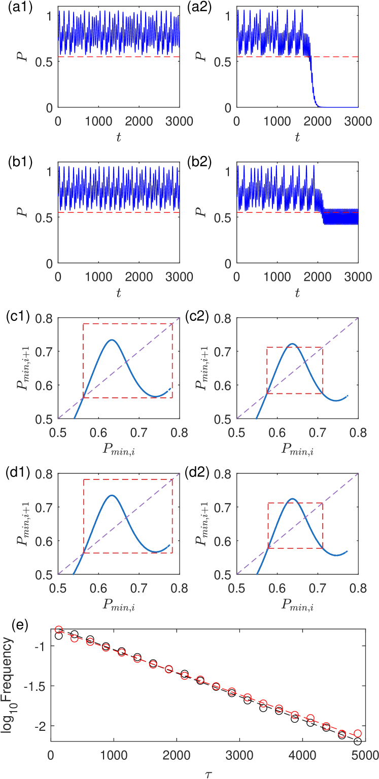
Figure 3: Predicting transient chaos and collapse of a food chain system. (a1,a2) Typical time series of the predator density $P$ in the normal and transient regimes, respectively, for $K=0.997<K_{c}$ and $K=1.01>K_{c}$. (b1,b2) Predicted time series of $P$ for the same values of $K$ as in (a1,a2), respectively. The machine predicts correctly the sudden collapse for $K>K_{c}$. (c1,c2) Return maps constructed from the local minima of $P(t)$ from the true time series, where the red dashed squares define an interval in which an invariant set exists: a chaotic attractor at $K=0.997<K_{c}$ (c1) or a nonattracting chaotic set at $K=1.01>K_{c}$ due to the escaping region about the critical point leading to transient chaos (c2). (d1,d2) Predicted return maps for the same values of $K$ as in (c1,c2), respectively. (e) Actual (black) and predicted (red) transient lifetime distributions at $K=K_{c}+2\times 10^{-4}$.

The second example is three-species food chain model McCann and Yodzis (1994b) where, as the environmental capacity $K$ of the resource species is varied, a catastrophic bifurcation and subsequent transient chaos leading to sudden species extinction occurs. The system equations, when being expanded into a power series, have an infinite number of nontrivial terms, violating the sparsity condition and rendering inapplicable any existing sparse optimization technique for data based discovery of the system equations (detailed in Sec. IIB in SI SI ). Figures 3(a1) and (a2) show typical behaviors of the predator density $P$ for $K<K_{c}$ and $K>K_{c}$ ($K_{c}=0.99976$), where there is sustained chaos in the former and transient chaos leading to species extinction in the latter. We train the reservoir machine at $K=0.97$, $0.98$, and $0.99$ - all in the sustained chaos regime. As shown in Figs. 3(b1) and (b2), the reservoir predicts correctly that, as the value of $K$ is increased, a catastrophic crisis will occur. Averaging over an ensemble of 500 different reservoir realizations, we obtain the predicted critical transition point as $K^{*}_{c}=0.9997\pm 4\times 10^{-4}$, which agrees well with the actual value $K_{c}=0.99976$. Figure 3(e) shows the predicted distribution of the transient lifetime obtained from 100 realizations of the reservoir machines, each with 400 random initial conditions. The predicted average transient lifetime is about $1.35\times 10^{3}$, which agrees well with the true value ($1.33\times 10^{3}$). All the transient lifetime are measured at values of $K$ that are $2\times 10^{-4}$ beyond the systems’ critical points.

If predicting system collapse is viewed as a binary classification problem (i.e., with or without collapse), it would be useful to train the neural machine with data from both below and above the critical point. A difficulty is that, beyond the critical point, the system will collapse after a transient chaotic phase of random duration. Practically, it is infeasible to obtain sufficient training data from the system in the post-critical regime. Moreover, our machine learning method can be used to assess the likelihood of the occurrence of a crisis in the near future where no post-critical data are available.

Our results suggest that the reservoir machine trained with data from a few distinct values of the bifurcation parameter represents a “regression” between the dynamical behavior of the target system and the bifurcation parameter. The machine is able to make statistically accurate predictions outside the training region. Since training is done on as few as three different values of the bifurcation parameter, the prediction of, e.g., the critical transition point, from any individual reservoir realization will involve large errors. However, the collective prediction from an ensemble of statistically independent reservoir machines can be quite accurate. (A further analysis of the reservoir performance is provided in Secs. VI-VII in SI SI .) In general, the prediction error would increase if the training parameter values are further from the critical transition point, suggesting that reservoir machines represent a low order approximation of the real dynamical systems about the training points of the bifurcation parameter. This is a natural and inevitable trade-off.

In summary, we have articulated a parameter-aware scheme of reservoir computing to predict collapse as a result of parameter drift driving the system into transient chaos by designating an additional input channel to accommodate the bifurcation parameter, which is equivalent to introducing adjustable biases between the input and the hidden layers. With parameter dependent training, all in the regime of sustained chaos, the reservoir machine acquires the ability to capture the variations in the “climate” of the target system, thereby gaining the power to predict the system state for different parameter values. When a parameter drift pushes the system through a critical point into a regime of transient chaos where collapse is inevitable, our design of machine learning is capable of accurate prediction of the critical value of the parameter, and of the statistical characteristics of transient chaos and the eventual collapse. These features are demonstrated using an electrical power system and a food-chain model in ecology. (An example of predicting transient spatiotemporal chaos in the Kuramoto-Sivashinsky system is given in Sec. III of SI SI .)

This work was supported by ONR under Grant No. N00014-16-1-2828.

References

- Dhamala and Lai (1999) M. Dhamala and Y.-C. Lai, Phys. Rev. E 59, 1646 (1999).
- McCann and Yodzis (1994a) K. McCann and P. Yodzis, Ame. Naturalist 144, 873 (1994a).
- Hastings et al. (2018) A. Hastings, K. C. Abbott, K. Cuddington, T. Francis, G. Gellner, Y.-C. Lai, A. Morozov, S. Petrivskii, K. Scranton, and M. L. Zeeman, Science 361, eaat6412 (2018).
- Grebogi et al. (1983) C. Grebogi, E. Ott, and J. A. Yorke, Physica D 7, 181 (1983).
- Wang et al. (2011) W.-X. Wang, R. Yang, Y.-C. Lai, V. Kovanis, and C. Grebogi, Phys. Rev. Lett. 106, 154101 (2011).
- Wang et al. (2016) W.-X. Wang, Y.-C. Lai, and C. Grebogi, Phys. Rep. 644, 1 (2016).
- Takens (1981) F. Takens, in Dynamical Systems and Turbulence, Lecture Notes in Mathematics, Vol. 898, edited by D. Rand and L. S. Young (Springer-Verlag, Berlin, 1981) pp. 366–381.
- Jaeger (2001) H. Jaeger, German National Research Center for Information Technology GMD Technical Report 148, 13 (2001).
- Mass et al. (2002) W. Mass, T. Nachtschlaeger, and H. Markram, Neur. Comp. 14, 2531 (2002).
- Jaeger and Haas (2004) H. Jaeger and H. Haas, Science 304, 78 (2004).
- Manjunath and Jaeger (2013) G. Manjunath and H. Jaeger, Neur. Comp. 25, 671 (2013).
- Haynes et al. (2015) N. D. Haynes, M. C. Soriano, D. P. Rosin, I. Fischer, and D. J. Gauthier, Phys. Rev. E 91, 020801 (2015).
- Larger et al. (2017) L. Larger, A. Baylón-Fuentes, R. Martinenghi, V. S. Udaltsov, Y. K. Chembo, and M. Jacquot, Phys. Rev. X 7, 011015 (2017).
- Pathak et al. (2017) J. Pathak, Z. Lu, B. Hunt, M. Girvan, and E. Ott, Chaos 27, 121102 (2017).
- Lu et al. (2017) Z. Lu, J. Pathak, B. Hunt, M. Girvan, R. Brockett, and E. Ott, Chaos 27, 041102 (2017).
- Duriez et al. (2017) T. Duriez, S. L. Brunton, and B. R. Noack, Machine Learning Control-Taming Nonlinear Dynamics and Turbulence (Springer, 2017).
- Lu et al. (2018) Z. Lu, B. R. Hunt, and E. Ott, Chaos 28, 061104 (2018).
- Pathak et al. (2018a) J. Pathak, A. Wilner, R. Fussell, S. Chandra, B. Hunt, M. Girvan, Z. Lu, and E. Ott, Chaos 28, 041101 (2018a).
- Pathak et al. (2018b) J. Pathak, B. Hunt, M. Girvan, Z. Lu, and E. Ott, Phys. Rev. Lett. 120, 024102 (2018b).
- Carroll (2018) T. L. Carroll, Phys. Rev. E 98, 052209 (2018).
- Nakai and Saiki (2018) K. Nakai and Y. Saiki, Phys. Rev. E 98, 023111 (2018).
- Roland and Parlitz (2018) Z. S. Roland and U. Parlitz, Chaos 28, 043118 (2018).
- Weng et al. (2019) T. Weng, H. Yang, C. Gu, J. Zhang, and M. Small, Phys. Rev. E 99, 042203 (2019).
- Griffith et al. (2019) A. Griffith, A. Pomerance, and D. J. Gauthier, Chaos 29, 123108 (2019).
- Jiang and Lai (2019) J. Jiang and Y.-C. Lai, Phys. Rev. Research 1, 033056 (2019).
- Vlachas et al. (2019) P. R. Vlachas, J. Pathak, B. R. Hunt, T. P. Sapsis, M. Girvan, E. Ott, and P. Koumoutsakos, arXiv preprint arXiv:1910.05266 (2019).
- Fan et al. (2020) H. Fan, J. Jiang, C. Zhang, X. Wang, and Y.-C. Lai, Phys. Rev. Research 2, 012080 (2020).
- Kuramoto (1978) Y. Kuramoto, Prog. Theo. Phys. Supp. 64, 346 (1978).
- Sivashinsky (1980) G. I. Sivashinsky, SIAM J. Appl. Math. 39, 67 (1980).
- Hyman et al. (1986) J. M. Hyman, B. Nicolaenko, and S. Zaleski, Physica D 23, 265 (1986).
- (31) The Supplementary Information provides additional details of the results in the main text. It is helpful but not essential for understanding the main rsults of the paper. It contains the following materials: a detailed description of the proposed parameter-aware reservoir computing machine, details of the model transient chaotic systems used in the main text, the issue of sensitivity to hyperparameters, the effects of input and reservoir matrices on performance, reservoir computing scheme with continuously varying bifurcation parameter, robustness against noise, and predicting transient spatiotemporal chaos and collapse in the one-dimensional Kuramoto-Sivashinsky system .
- Ikeda (1979) K. Ikeda, Opt. Commun. 30, 257 (1979).
- Ikeda et al. (1980) K. Ikeda, H. Daido, and O. Akimoto, Phys. Rev. Lett. 45, 709 (1980).
- Hammel et al. (1985) S. M. Hammel, C. K. R. T. Jones, and J. V. Moloney, J. Opt. Soc. Ame. B 2, 552 (1985).
- In et al. (1998) V. In, M. L. Spano, and M. Ding, Phys. Rev. Lett. 80, 700 (1998).
- McCann and Yodzis (1994b) K. McCann and P. Yodzis, Ame. Naturalist 144, 873 (1994b).