Measuring correlated electron motion in atoms with the momentum-balance density

Abstract

Three new measures of relative electron motion are introduced: equimomentum, antimomentum, and momentum-balance. The equimomentum is the probability that two electrons have the exact same momentum, whereas the antimomentum is the probability their momenta are the exact opposite. Momentum-balance (MB) is the difference between the equimomentum and antimomentum, and therefore indicates if equal or opposite momentum is more probably in a system of electrons. The equimomentum, antimomentum and MB densities are also introduced, which are the local contribution to each quantity. The MB and MB density of the extrapolated-Full Configuration Interaction wave functions of atoms of the first three rows of the periodic table are analyzed, with a particular focus on contrasting the correlated motion of electrons with opposite and parallel spin. Coulomb correlation between opposite-spin electrons leads to a higher probability of equimomentum, whereas Fermi correlation between parallel-spin electrons leads to a higher probability of antimomentum. The local contribution to MB, given an electron is present, is a minimum at the nucleus and generally increases as the distance from the nucleus increases. There are also interesting similarities between the effects of Fermi correlation and Coulomb correlation (of opposite-spin electrons) on MB.

I Introduction

Most of the difficulties encountered in the study of electronic structure, both experimentally and computationally, arise from the complexity of the many-electron wave function. Therefore, both stand to benefit substantially from the unravelling this complexity. The unravelling can begin by understanding the relative motion of electrons. Not only does this help demystify the mesmerizing many-electron wave function, but it also lends itself to the development of more suitable models of electronic structure and a more complete picture of quantum mechanics.

Much has been learned about the relative position and momentum of electrons, and most is due to the analysis of intracules.Coulson and Neilson (1961); Lester Jr and Krauss (1966); Coleman (1967); Banyard and Ellis (1972); Thakkar and Smith Jr. (1977); Banyard and Reed (1978); Sharma and Thakkar (1984); Thakkar, Tripathi, and Smith Jr (1984); Boyd, Sarasola, and Ugalde (1988); Wang, Tripathi, and Smith Jr (1992); Dominguez et al. (1992); Aguado et al. (1992); Sarasola et al. (1992); Banyard and Sanders (1993); Cann, Boyd, and Thakkar (1993a, b, c); Cioslowski and Liu (1996); Fradera, Duran, and Mestres (1997); Sarsa, Gálvez, and Buendia (1998, 1999); Fradera, Duran, and Mestres (2000); Koga (2001, 2002); Koga and Matsuyama (2003); Gill, O’Neill, and Besley (2003); Toulouse, Assaraf, and Umrigar (2007); Dumont, Crittenden, and Gill (2007); Crittenden, Dumont, and Gill (2007); Crittenden and Gill (2007); Bernard, Crittenden, and Gill (2008); Piris, Lopez, and Ugalde (2008); Pearson et al. (2009); Per, Russo, and Snook (2009); Hollett and Gill (2011); Loos and Gill (2010); Hollett, McKemmish, and Gill (2011); Hollett and Gill (2012); Bernard, Loos, and Gill (2013); Mercero et al. (2016); Hollett and Li (2017); Rodríguez-Mayorga et al. (2018, 2019); Via-Nadal et al. (2019) Intracules are two-electron probability distribution functions.Gill et al. (2006) Constructed from the $N$-electron wave function (approximate or exact), these reduced probability densities reveal information regarding the relative position,Coulson and Neilson (1961); Banyard and Ellis (1972); Sharma and Thakkar (1984); Koga (2002); Hollett and Gill (2012) momentum,Banyard and Ellis (1972); Banyard and Reed (1978); Koga (2002); Hollett and Gill (2012) or position and momentum of electrons.Gill and Chien (2003); Bernard, Loos, and Gill (2013) The analyses often involve the calculation of intracule holes,Coulson and Neilson (1961); Cioslowski and Liu (1998) which are the difference between the exact and the Hartree-Fock intracule. An intracule hole explicitly describes the effects of Coulomb correlationTew, Klopper, and Helgaker (2007) on that particular intracule, and subsequent inferences are made regarding the correlated motion of the electrons. Such studies have led to a better understanding of the relative motion of electrons due to radial and angular correlation in atoms,Banyard and Ellis (1972); Hollett, McKemmish, and Gill (2011); Hollett and Gill (2012) the correlated motion of electrons during bond dissociation,Hollett, McKemmish, and Gill (2011) and their correlated motion in the presence of a static electric field.Hollett and Li (2017) However, for most intracules the spatial information (i.e. absolute location of the electrons) is lost, which impedes the completion of a picture of relative electron motion in atoms and molecules.

By using a more complex object, such as the two-electron density, correlated electron movement can be analyzed in real space through the construction of Coulomb,Sanders and Banyard (1992); Banyard and Sanders (1993) exchange, or exchange-correlationWang, Kim, and Baerends (2010) holes. In this context, the hole is the two-electron density as a function of the position of the second electron when a test position is chosen for the first.Cooper and Pounder (1978); Tew, Klopper, and Helgaker (2007) Such an approach can be used to demonstrate Fermi correlation and the Fermi hole, which occur between electrons of parallel-spin and is due to the antisymmetry of the electronic wave function.Tew, Klopper, and Helgaker (2007) This approach is also used to design and test models for density functional approximations.Baerends (2001) By choosing a position in the molecule for the test electron, the complexity of the two-electron density is reduced but a complete picture of the relative motion of the electrons must be synthesized from the combination of densities produced from a collection of test electron positions.

Alternatively, there are intracule-like probability densities that are not reduced to a single (1D or 3D) variable. Such probability densities, like the intex distribution,Proud and Pearson (2010, 2012); Valderrama, Mercero, and Ugalde (2001) retain absolute position information, that is often lost with simpler intracules, and can provide information regarding the relative positions of electrons at different locations in an atom or molecule. Similar distributions also exist for momentum space.Reed and Banyard (1980)

In an effort to unravel some of the complexity of the correlated motion of electrons this article presents multiple new quantum mechanical properties. The properties are the equi- and antimomentum and momentum-balance, along with the corresponding equi- and antimomentum density and momentum-balance density. The momentum-balance is a measure of the correlated motion in an electronic system, and the momentum-balance density describes the local contribution of the electronic wave function to the correlated electron motion. In Section II, expressions for the equimomentum, antimomentum, and momentum balance are derived, along with the corresponding densities. This is followed by a description of the basic algorithm for the calculation of these properties in atoms and molecules using Gaussian basis sets. Section IV presents an analysis and discussion of the momentum-balance and momentum-balance density in atoms of the first 17 many-electron elements of the periodic table. Then finally, the results are summarized and future applications of these properties are discussed in Section V. Atomic units are used throughout.

II Theory

The connection between electron position and momentum is through the Fourier transform. The $N$-electron momentum-space wave function, $\Phi$, in terms of the position-space wave function, $\Psi$, is given as

$$\Phi(\mathbf{p}_{1},\mathbf{p}_{2},\dots,\mathbf{p}_{N})=\frac{1}{(2\pi)^{3N}}\int e^{-i\sum_{k=1}^{N}\mathbf{p}_{k}\cdot\mathbf{r}_{k}}\\ \times\Psi(\mathbf{r}_{1},\mathbf{r}_{2},\dots,\mathbf{r}_{N})d\mathbf{r}_{1}d\mathbf{r}_{2}\dots d\mathbf{r}_{N},$$ (1)

where $\mathbf{p}_{k}$ and $\mathbf{r}_{k}$ are the electron momenta and positions, respectively. The wave functions are spinless, that is, they have been previously integrated with respect to the electron spin-coordinates. When addressing the relative motion of electrons, it is simpler to focus on electron pairs rather than all $N$-electrons at once. Therefore, the two-electron reduced density matrix (2-RDM), $\Gamma(\mathbf{r}_{1},\mathbf{r}_{2},\mathbf{r}_{1}^{\prime},\mathbf{r}_{2}^{\prime})$, is formed via integration over the $N$-electron wave function,

$$\Gamma(\mathbf{r}_{1},\mathbf{r}_{2},\mathbf{r}_{1}^{\prime},\mathbf{r}_{2}^{\prime})=\int\Psi^{*}(\mathbf{r}_{1}^{\prime},\mathbf{r}_{2}^{\prime},\dots,\mathbf{r}_{N})\\ \times\Psi(\mathbf{r}_{1},\mathbf{r}_{2},\dots,\mathbf{r}_{N})d\mathbf{r}_{3}\dots d\mathbf{r}_{N},$$ (2)

where the diagonal of the 2-RDM is the two-electron density, $\Gamma(\mathbf{r}_{1},\mathbf{r}_{2})=\Gamma(\mathbf{r}_{1},\mathbf{r}_{2},\mathbf{r}_{1},\mathbf{r}_{2})$. Following Equation (1), the two-electron momentum density, $\Pi(\mathbf{p}_{1},\mathbf{p}_{2})$, can be formed from the position-space 2-RDM,

$$\Pi(\mathbf{p}_{1},\mathbf{p}_{2})=\frac{1}{(2\pi)^{6}}\int e^{i\left[\mathbf{p}_{1}\cdot(\mathbf{r}_{1}^{\prime}-\mathbf{r}_{1})+\mathbf{p}_{2}\cdot(\mathbf{r}_{2}^{\prime}-\mathbf{r}_{2})\right]}\\ \times\Gamma(\mathbf{r}_{1},\mathbf{r}_{2},\mathbf{r}_{1}^{\prime},\mathbf{r}_{2}^{\prime})d\mathbf{r}_{1}d\mathbf{r}_{2}d\mathbf{r}_{1}^{\prime}d\mathbf{r}_{2}^{\prime}.$$ (3)

The two-electron momentum density gives the simultaneous probability that one electron has momentum $\mathbf{p}_{1}$ and another has $\mathbf{p}_{2}$. By inserting a Dirac delta function, $\delta(x)$, and using the identity, $\delta(x)=\frac{1}{2\pi}\int e^{-ikx}dk$, the probability that two electrons have the exact same momentum can be calculated,

$$\lambda^{+}= \int\Pi(\mathbf{p}_{1},\mathbf{p}_{2})\delta(\mathbf{p}_{1}-\mathbf{p}_{2})d\mathbf{p}_{1}d\mathbf{p}_{2}$$

$$= \frac{1}{(2\pi)^{3}}\int\Gamma(\mathbf{r}_{1},\mathbf{r}_{2},\mathbf{r}_{1}+\mathbf{q},\mathbf{r}_{2}-\mathbf{q})d\mathbf{q}d\mathbf{r}_{1}d\mathbf{r}_{2},$$ (4)

which will be referred to as the equimomentum. Similarly, the probability that two electrons have the exact opposite momentum is given by,

$$\lambda^{-}= \int\Pi(\mathbf{p}_{1},\mathbf{p}_{2})\delta(\mathbf{p}_{1}+\mathbf{p}_{2})d\mathbf{p}_{1}d\mathbf{p}_{2}$$

$$= \frac{1}{(2\pi)^{3}}\int\Gamma(\mathbf{r}_{1},\mathbf{r}_{2},\mathbf{r}_{1}+\mathbf{q},\mathbf{r}_{2}+\mathbf{q})d\mathbf{q}d\mathbf{r}_{1}d\mathbf{r}_{2},$$ (5)

which will be referred to as the antimomentum. The difference between the two, will be referred to as the momentum-balance (MB),

$$\mu=\lambda^{+}-\lambda^{-}$$ (6)

The MB is positive for a system in which it is more probable that the electrons have the same momentum, negative for a system in which opposite momenta are more probable, and zero when both scenarios are equally likely.

If the integrand for the equi- or antimomentum [Equation (II) or (II)] is integrated over only one of the electron coordinates the result is the local contribution to each quantity,

$$\lambda^{\pm}(\mathbf{r})=\frac{1}{(2\pi)^{3}}\int\Gamma(\mathbf{r},\mathbf{r}_{2},\mathbf{r}+\mathbf{q},\mathbf{r}_{2}\mp\mathbf{q})d\mathbf{r}_{2}d\mathbf{q},$$ (7)

the equimomentum density, $\lambda^{+}(\mathbf{r})$, and the antimomentum density, $\lambda^{-}(\mathbf{r})$. The difference between the two is the MB density,

$$\mu(\mathbf{r})=\lambda^{+}(\mathbf{r})-\lambda^{-}(\mathbf{r})$$ (8)

Although $\lambda^{+}(\mathbf{r})$ and $\lambda^{-}(\mathbf{r})$ are not probability densities, the MB density can still be analyzed to reveal the regions of a wave function that contribute to electrons having equal or opposite momenta. Such analysis is analogous to that seen with various types of energy densities.Ayers, Parr, and Nagy (2002); Anderson, Ayers, and Hernandez (2010); Bacskay and Nordholm (2017) The sign of the MB density reveals whether there is a local contribution to equi- or antimomentum,

$$\mu(\mathbf{r})>0\> \implies$$ contributes to equal momenta

$$\mu(\mathbf{r})<0\> \implies$$ contributes to opposite momenta

Inspection of the definitions of $\lambda^{+}(\mathbf{r})$ and $\lambda^{-}(\mathbf{r})$ [Equation (S11)] in terms of the 2-RDM reveals a strong dependence of those densities and the MB density on the electron density at $\mathbf{r}$. Therefore, a reduced MB density, $m(\mathbf{r})$, is defined (similar to an energy potential) to eliminate that dependence,

$$m(\mathbf{r})=\frac{\mu(\mathbf{r})}{\rho(\mathbf{r})},$$ (9)

where $\rho(\mathbf{r})$ is the one-electron density. It is expected that $m(\mathbf{r})$ will reveal more fine details of the relative momenta of electrons in a system in comparison to $\mu(\mathbf{r})$.

For wave functions constructed from an orbital basis, the equi- and antimomentum can be calculated by contracting the 2-RDM in the given basis, $\Gamma_{abcd}$, with the appropriate two-electron integrals,

$$\lambda^{\pm}=\sum_{abcd}\Gamma_{abcd}\left[abcd\right]_{\lambda^{\pm}}.$$ (10)

The two-electron integrals are given by

$$\left[abcd\right]_{\lambda^{\pm}}=\frac{1}{(2\pi)^{3}}\int\phi_{a}(\mathbf{r}_{1})\phi_{b}(\mathbf{r}_{1}+\mathbf{q})\\ \times\phi_{c}(\mathbf{r}_{2})\phi_{d}(\mathbf{r}_{2}\mp\mathbf{q})d\mathbf{q}d\mathbf{r}_{1}d\mathbf{r}_{2},$$ (11)

where the orbitals, $\phi_{a}$, are assumed to be real. The integrals exhibit the very practical identity,

$$\left[abcd\right]_{\lambda^{-}}=\left[abdc\right]_{\lambda^{+}}.$$ (12)

The equi- and antimomentum densities can be calculated in the same manner, except the four-orbital integral is replaced by the product of an orbital and a three-orbital integral,

$$\lambda^{\pm}(\mathbf{r})=\sum_{abcd}\Gamma_{abcd}\phi_{a}(\mathbf{r})\left[bcd\right]_{\lambda^{\pm}}.$$ (13)

The three-orbital integral is given by,

$$\left[bcd\right]_{\lambda^{\pm}}=\frac{1}{(2\pi)^{3}}\int\phi_{b}(\mathbf{r}+\mathbf{q})\\ \times\phi_{c}(\mathbf{r}_{2})\phi_{d}(\mathbf{r}_{2}\mp\mathbf{q})d\mathbf{q}d\mathbf{r}_{2}$$ (14)

which also has a useful identity,

$$\left[bcd\right]_{\lambda^{-}}=\left[bdc\right]_{\lambda^{+}}.$$ (15)

Recurrence relations for the practical calculation of the molecular integrals, $\left[abcd\right]_{\lambda^{\pm}}$ and $\left[bcd\right]_{\lambda^{\pm}}$, over Gaussian-type basis functions of arbitrary angular momentum are provided in the supplementary material.

Analysis of the relative motion of electrons via MB and the MB density, is aided by decomposing the 2-RDM into its various spin-components,

$$\Gamma(\mathbf{r}_{1},\mathbf{r}_{2},\mathbf{r}_{1}^{\prime},\mathbf{r}_{2}^{\prime})= \Gamma^{\alpha\alpha}(\mathbf{r}_{1},\mathbf{r}_{2},\mathbf{r}_{1}^{\prime},\mathbf{r}_{2}^{\prime})+\Gamma^{\beta\beta}(\mathbf{r}_{1},\mathbf{r}_{2},\mathbf{r}_{1}^{\prime},\mathbf{r}_{2}^{\prime})$$

$$\Gamma^{\alpha\beta}(\mathbf{r}_{1},\mathbf{r}_{2},\mathbf{r}_{1}^{\prime},\mathbf{r}_{2}^{\prime})+\Gamma^{\beta\alpha}(\mathbf{r}_{1},\mathbf{r}_{2},\mathbf{r}_{1}^{\prime},\mathbf{r}_{2}^{\prime}),$$ (16)

where $\alpha$ denotes “spin-up” and $\beta$ denotes ”spin-down”. To demonstrate the relationship between $\mu$ and correlated electron motion, consider the Hartree-Fock wave function. Inserting the spin-resolved HF 2-RDM into Equation (S12) yields an expression for the HF equi- and antimomentum,

$$\lambda^{\pm}_{\text{HF}}=\frac{1}{2}\sum_{ij}n^{\alpha}_{i}n^{\alpha}_{j}\left(\left[iijj\right]^{\alpha\alpha}_{\lambda^{\pm}}-\left[ijji\right]^{\alpha\alpha}_{\lambda^{\pm}}\right)\\ +n^{\beta}_{i}n^{\beta}_{j}\left(\left[iijj\right]^{\beta\beta}_{\lambda^{\pm}}-\left[ijji\right]^{\beta\beta}_{\lambda^{\pm}}\right)\\ +n^{\alpha}_{i}n^{\beta}_{j}\left(\left[iijj\right]^{\alpha\beta}_{\lambda^{\pm}}+\left[iijj\right]^{\beta\alpha}_{\lambda^{\pm}}\right),$$ (17)

where $n_{i}^{\sigma}$ is the occupancy of $\sigma$-spin orbital $i$, with $\sigma=\alpha$ or $\beta$. The integral identity relating equimomentum and antimomentum [Equation (S9)] implies that the Coulomb-type integral for both quantities are equivalent,

$$\left[iijj\right]_{\lambda^{-}}=\left[iijj\right]_{\lambda^{+}}.$$ (18)

Considering this, and the decomposition of $\mu$ into spin-components,

$$\mu_{\text{HF}}=\mu^{\alpha\alpha}_{\text{HF}}+\mu^{\beta\beta}_{\text{HF}}+\mu^{\alpha\beta}_{\text{HF}}+\mu^{\beta\alpha}_{\text{HF}},$$ (19)

the following simplification can be made,

$$\mu^{\sigma\sigma}_{\text{HF}}=\frac{1}{2}\sum_{ij}n^{\sigma}_{i}n^{\sigma}_{j}\left(\left[ijji\right]^{\sigma\sigma}_{\lambda^{-}}-\left[ijji\right]^{\sigma\sigma}_{\lambda^{+}}\right).$$ (20)

The HF MB between electrons of parallel-spin is the difference between the equi- and antimomentum contributions that result from the exchange interaction (i.e. antisymmetry). Given that there is no exchange interaction between electrons of opposite-spin, the HF MB of opposite-spin electrons is exactly zero,

$$\mu^{\sigma\sigma^{\prime}}_{\text{HF}}=0.$$ (21)

An analogous result is found for the MB density,

$$\mu^{\sigma\sigma}_{\text{HF}}(\mathbf{r})=\frac{1}{2}\sum_{ij}n^{\sigma}_{i}n^{\sigma}_{j}\phi_{i}^{\sigma}(\mathbf{r})\left(\left[jji\right]^{\sigma\sigma}_{\lambda^{-}}-\left[jji\right]^{\sigma\sigma}_{\lambda^{+}}\right),$$ (22)

and

$$\mu^{\sigma\sigma^{\prime}}_{\text{HF}}(\mathbf{r})=0.$$ (23)

It is clear from this result that non-zero MB and MB density only exists when electron motion is correlated. In other words, if electron motion is uncorrelated then equimomentum and antimomentum are equally probable, $\lambda^{+}=\lambda^{-}$ and $\lambda^{+}(\mathbf{r})=\lambda^{-}(\mathbf{r})$. In the case of the HF wave function, correlation occurs only between parallel-spin electrons and is due to the antisymmetry of the wave function, often referred to as Fermi correlation.Tew, Klopper, and Helgaker (2007) Therefore, the MB and MB density of correlated (e.g. post-HF) wave functions reveal the presence of correlation between opposite-spin electrons and the change in correlation between parallel-spin electrons.

III Method

All wave functions (including 1 and 2-RDMs) were obtained using a determinant-driven selected configuration interaction (sCI) method known as CIPSI (Configuration Interaction using a Perturbative Selection made Iteratively)Huron, Malrieu, and Rancurel (1973); Giner, Scemama, and Caffarel (2013, 2015) in which the energies are extrapolated to the full configuration interaction (FCI) result using multireference perturbation theory.Garniron et al. (2017); Loos et al. (2018); Garniron et al. (2019) The all-electron extrapolated-FCI (exFCI) calculations were performed using Quantum Package 2.0.Garniron et al. (2019) The wave functions and RDMs for He were obtained using the cc-pVTZ, aug-cc-pVTZ and aug-cc-pVQZ/f basis sets,Dunning Jr. (1989); Woon and Dunning Jr. (1994) and all calculations beyond He were performed using the aug-cc-pCVTZ/f basis set.Prascher et al. (2011); Feller (1996); Schuchardt et al. (2007); Pritchard et al. (2019)

Using the RDMs provided by Quantum Package 2.0, the equimomentum, antimomentum, and MB, along with their densities were calculated using MUNgauss.Poirier, Hollett, and Warburton (2015) The densities were calculated on a two-dimensional mesh, with a grid-spacing of 0.05 bohr, for visualization. The densities were also numerically integrated on the SG-1 gridGill, Johnson, and Pople (1993) for comparison to analytically calculated equimomentum, antimomentum and MB values.

IV Results

IV.1 Opposite-spin correlation

As an initial assessment of basis set dependence, the MB density of the He atom obtained using three different Dunning basis sets is shown in Figure 1.

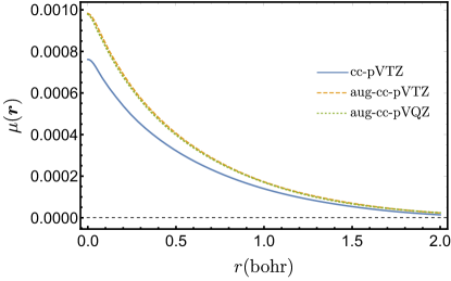
Figure 1: Comparison of momentum-balance density of He atom for multiple Dunning correlation-consistent basis sets.

It is seen that there is significant deviation between the MB density calculated using the cc-pVTZ basis set and the density calculated using the aug-cc-pVTZ basis set. The deviation is most pronounced at the nucleus and decays as the distance from the nucleus increases. Therefore, it appears the addition of diffuse functions, or “augmenting” the basis set, (cc-pVTZ to aug-cc-pVTZ) is more important to an accurate description of the MB density than adding an extra set of valence basis functions (aug-cc-pVTZ to aug-cc-pVQZ). Furthermore, the MB density is far more sensitive to basis set than the one-electron density (Figure 2). This may not be surprising considering it is a comparison between a one-electron property and a two-electron property. All subsequent properties of He that follow are obtained using the aug-cc-pVQZ basis set.

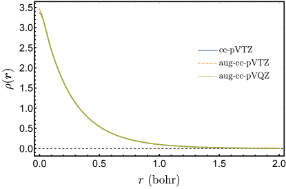
Figure 2: Comparison of total one-electron density of He atom for multiple Dunning correlation-consistent basis sets.

In Figure 3, the He atom MB density, $\mu(\mathbf{r})$, reduced MB density, $m(\mathbf{r})$, and one-electron density, $\rho(\mathbf{r})$ are plotted together.

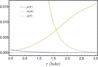
Figure 3: Total momentum-balance density and reduced momentum-balance density of He, with the one-electron density.

Evident from Figures 1 and 3, $\mu(\mathbf{r})$ for He is positive everywhere, and results in a total MB of 0.00373. The MB is the difference between an equimomentum $\lambda^{+}=0.02481$ and an antimomentum $\lambda^{-}=0.02107$. In other words, if one could measure the simultaneous momenta of the two electrons of ground state He 100 000 times, they would find the electrons have the exact same momentum 2 481 times and the exact opposite momentum 2 107 times. The difference, which is the MB, is due to Coulomb correlation between the $\alpha$ and $\beta$ electron. Their correlated motion favours equimomentum over antimomentum, which is consistent with earlier studies of angular correlation in the He atom.Banyard and Reed (1978); Koga and Matsuyama (2003); Hollett and Gill (2012)

From Figures 1 and 2 it is clear that $\mu(\mathbf{r})$ closely follows the shape of the $\rho(\mathbf{r})$, albeit with a much smaller magnitude and slower decay. As mentioned previously, this is due to the dependence of the two-electron density on the one-electron density (i.e. an electron must be present to interact). This dependency is removed in the reduced MB density, $m(\mathbf{r})$, which can be viewed as a MB potential. It is seen that $m(\mathbf{r})$ is actually a minimum at the nucleus and the potential contribution to MB increases as the distance from the nucleus increases. Of course, while $m(\mathbf{r})$ continues to grow as $r$ increases, $\rho(\mathbf{r})$ decays and eventually extinguishes the contribution.

Figure 4 presents the $\alpha\beta$ MB density of He, Li and Be divided by the number of $\alpha\beta$ electron pairs.

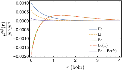
Figure 4: Renormalized $\mu^{\alpha\beta}(\mathbf{r})$ of He, Li, Be and Be(fc) [frozen core]. The difference between the all-electron and frozen core $\mu^{\alpha\beta}(\mathbf{r})$ for Be is included.

It also includes $\mu^{\alpha\beta}(\mathbf{r})$ of Be calculated using a frozen-core approximation to ascertain the role of the valence electrons in $\mu^{\alpha\beta}(\mathbf{r})$. The frozen-core $\mu^{\alpha\beta}(\mathbf{r})$ closely resembles the fully correlated $\mu^{\alpha\beta}(\mathbf{r})$ which, unlike He and Li, has a node at small $r$ and a negative peak at the nucleus. It is evident that the valence electrons are mainly responsible for the structure of $\mu^{\alpha\beta}(\mathbf{r})$ for Be. The difference between the frozen-core and fully correlated $\mu^{\alpha\beta}(\mathbf{r})$ reveals the contribution from the core, and core-valence, correlation and it is very similar to the $\mu^{\alpha\beta}(\mathbf{r})$ of He and Li.

The reduced MB densities, divided by the number of $\beta$ electrons, of Be, Li and He are presented in Figure 5. Note, that for the spin-decomposed reduced MB density, $m^{\sigma\sigma^{\prime}}(\mathbf{r})=\frac{m^{\sigma\sigma^{\prime}}(\mathbf{r})}{\rho^{\sigma}(\mathbf{r})}$.

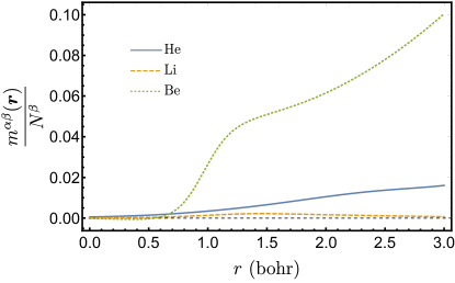
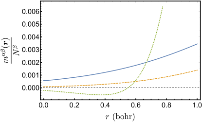
Figure 5: Renormalized $m^{\alpha\beta}(\mathbf{r})$ of He, Li, and Be.

The $m^{\alpha\beta}(\mathbf{r})$ are similar, in that they have a minimum at the nucleus and are everywhere positive. However, the $m^{\alpha\beta}(\mathbf{r})$ of Li reaches a maximum at $\sim$1.4 bohr and then decays due to the fact that $\rho^{\alpha}(\mathbf{r})$ decays much slower than $\rho^{\beta}(\mathbf{r})$, unlike He and Be. The amplitude of the Be $m^{\alpha\beta}(\mathbf{r})$, which is dominated by the valence electrons, is significantly larger than that of He and Li. Near the nucleus $m^{\alpha\beta}(\mathbf{r})$ of Be is negative and relatively flat. It reaches a minimum at 0.374 bohr and has node at 0.549 bohr. After crossing the node, $m^{\alpha\beta}(\mathbf{r})$ increases sharply with a shoulder just beyond $r=1$ bohr. The $m^{\alpha\beta}(\mathbf{r})$ of He also exhibits a shoulder, although it is less pronounced and further from the nucleus ($\sim$ 2.4 bohr).

The $\mu^{\alpha\beta}(\mathbf{r})$ for Be to Ne are presented in Figure 6.

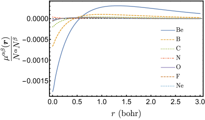
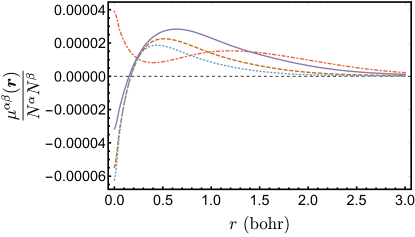
Figure 6: Renormalized $\mu^{\alpha\beta}(\mathbf{r})$ of the atoms Be to Ne (above) and N to Ne (below).

With the exception of N, all the atoms have a $\mu^{\alpha\beta}(\mathbf{r})$ with the the same shape as that of Be. Proceeding from Be to C the amplitude per $\alpha\beta$ electron pair decreases and the node contracts toward the nucleus, in the same manner as the node of a 2$s$ atomic orbital with increasing nuclear charge. Interestingly, $\mu^{\alpha\beta}(\mathbf{r})$ for the N atom has a positive peak at the nucleus, a minimum near $r=0.3$ bohr, and is positive everywhere. This indicates a reduction in the type of correlated motion between the valence electrons, exhibited by the electrons of Be to C, to such an extent that other correlated motion dominates $\mu^{\alpha\beta}(\mathbf{r})$, such as the relative motion of core, and core-valence electron pairs. With the addition of $\beta$-spin $p$-electrons, the $\mu^{\alpha\beta}(\mathbf{r})$ of O to Ne have a shape similar to the $\mu^{\alpha\beta}(\mathbf{r})$ of those atoms before N. From O to Ne, the amplitude of the maximum per electron pair decreases, while the amplitude of the minimum at the nucleus increases, and the location of the node remains relatively stationary.

For a description of the correlated momemnta that is unbiased by $\rho^{\alpha}(\mathbf{r})$, the reduced MB densities, divided by the number of $\beta$ electrons, of Be to Ne are presented in Figure 7.

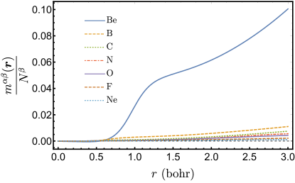
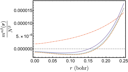
Figure 7: Renormalized $m^{\alpha\beta}(\mathbf{r})$ of the atoms Be to Ne (above) and N to Ne (below).

As expected from the analysis of $\mu^{\alpha\beta}(\mathbf{r})$, all $m^{\alpha\beta}(\mathbf{r})$ have the same shape with the exception of that for N, which is positive everywhere. The amplitude of $m^{\alpha\beta}(\mathbf{r})/N^{\beta}$ decreases substantially moving from Be to C. Far from the nucleus ($r>1.5$ bohr), the magnitude of $m^{\alpha\beta}(\mathbf{r})/N^{\beta}$ also decreases from O to Ne. However, the amplitude of $m^{\alpha\beta}(\mathbf{r})/N^{\beta}$ near the nucleus is less ordered.

The $\mu^{\alpha\beta}(\mathbf{r})$, per $\alpha\beta$ electron pair, for the third period atoms are presented in Figure 8.

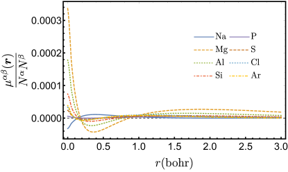
Figure 8: Renormalized $\mu^{\alpha\beta}(\mathbf{r})$ of the atoms Na to Ar.

The shape of $\mu^{\alpha\beta}(\mathbf{r})$ for the Na atom is the same as that for Ne. This is due to the fact that the $\beta$-electron configuration remains the same. Once a $\beta$ electron is added (Mg atom and beyond), the magnitude of $\mu^{\alpha\beta}(\mathbf{r})$ per $\alpha\beta$ electron pair increases substantially, similar to that seen for Be in the second period. Unlike atoms of the second period, the $\mu^{\alpha\beta}(\mathbf{r})$ of Mg and beyond have two nodes (like the $3s$ atomic orbital) and are positive at the nucleus. Yet again, like the second period atoms, $\mu^{\alpha\beta}(\mathbf{r})>0$ in the valence region and beyond.

The $\alpha\beta$ reduced MB densities, per $\beta$ electron, for the third period atoms are presented in Figure 9.

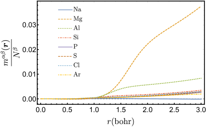
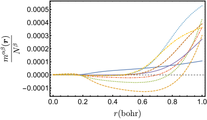
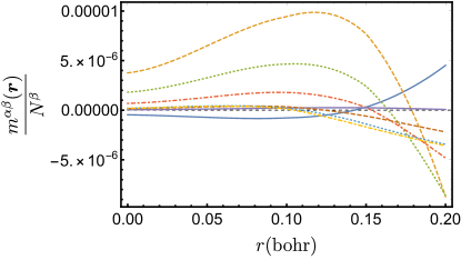
Figure 9: Renormalized $m^{\alpha\beta}(\mathbf{r})$ of the atoms Na to Ar.

As suggested by their $\mu^{\alpha\beta}(\mathbf{r})$, the $m^{\alpha\beta}(\mathbf{r})$ of Na closely resembles that of Ne. The $m^{\alpha\beta}(\mathbf{r})$ of Mg, like Be of the second period, has the the largest amplitude per $\beta$ electron. Close to the nucleus, the features of $m^{\alpha\beta}(\mathbf{r})$ are the same as those for the second period atoms, except the sign is reversed. These features are nested inside the same features (a minimum and a node) repeated, but with the same sign as those of the second period atoms. It is also interesting to note that, unlike N, the $m^{\alpha\beta}(\mathbf{r})$ for the $\ce{P}$ atom has the same number of nodes as the other atoms of the period. However, like N, the amplitude of $m^{\alpha\beta}(\mathbf{r})$ for P is relatively minuscule.

The trend in $\mu^{\alpha\beta}$ for the second and third period atoms is illustrated in Figure 10.

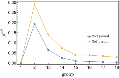
Figure 10: Opposite-spin momentum-balance of 2nd and 3rd row atoms.

For all atoms $\mu^{\alpha\beta}>0$, which corresponds to opposite-spin electrons preferring to have the same momentum rather than opposite, and periodicity is followed quite closely. There is a sharp increase in $\mu^{\alpha\beta}$ moving from group 1 to 2 (i.e. one valence electron to two) which illustrates the importance of valence electron motion to $\mu^{\alpha\beta}$. As atomic number increases, and more electrons are added to the valence shell, the value of $\mu^{\alpha\beta}$ decreases, which suggests less correlated motion.

For open-shell systems $\mu^{\alpha\beta}(\mathbf{r})\neq\mu^{\beta\alpha}(\mathbf{r})$, and subsequently $m^{\alpha\beta}(\mathbf{r})\neq m^{\beta\alpha}(\mathbf{r})$. However, the features observed in $\alpha\beta$ densities are very similar to those observed in the $\beta\alpha$ densities. Therefore, plots of $\mu^{\beta\alpha}(\mathbf{r})$ and $m^{\beta\alpha}(\mathbf{r})$ can be found in the supplementary material.

IV.2 Parallel-spin correlation

As mentioned previously, Fermi correlation contributes to the MB of parallel-spin electrons. Not surprisingly, the contribution of Fermi correlation is orders of magnitude larger than that of Coulomb correlation. Consider the Ne atom, where $\mu_{\text{HF}}^{\sigma\sigma}(\mathbf{r})=-0.08644$ and $\mu^{\sigma\sigma}(\mathbf{r})=-0.08663$, which means Coulomb correlation contributes $\sim$0.2% to the overall parallel-spin MB. Furthermore, Fermi correlation favours $\mu^{\sigma\sigma}<0$, which is parallel-spin electrons having the exact opposite momentum.

The $\alpha\alpha$ MB density per electron pair, $\frac{\mu^{\alpha\alpha}(\mathbf{r})}{N^{\alpha}(N^{\alpha}-1)/2}$, for atoms of the second period are presented in Figure 11.

Figure 11: Renormalized $\mu^{\alpha\alpha}(\mathbf{r})$ of the atoms Li to Ne.

It is seen that $\mu^{\alpha\alpha}(\mathbf{r})$ is negative everywhere, meaning all regions contribute to electrons having the exact opposite momentum. Similar to the opposite-spin MB density, the amplitude of $\mu^{\alpha\alpha}(\mathbf{r})$ is relatively small for Li. For the Be atom, which has only one valence $\alpha$-electron, the amplitude of $\mu^{\alpha\alpha}(\mathbf{r})$ is much more appreciable. But, it is still significantly smaller than that for atoms with multiple valence $\alpha$-electrons. The addition of $p$-electrons for B, and the proceeding atoms, creates a shoulder in $\mu^{\alpha\alpha}(\mathbf{r})$ further from the nucleus. Moving from B to Ne the shoulder contracts to the nucleus and the amplitude of $\mu^{\alpha\alpha}(\mathbf{r})$ per electron pair decreases.

Figure 12 presents the $\alpha\alpha$ reduced MB density, divided by the number of $\alpha$ electrons, for the second period atoms.

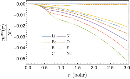
Figure 12: Renormalized $m^{\alpha\alpha}(\mathbf{r})$ of the atoms Li to Ne.

The amplitude of $m^{\alpha\alpha}(\mathbf{r})/N^{\alpha}$ increases slightly from Li to Be, and then substantially from Be to B. This is accompanied by a change in the shape of $m^{\alpha\alpha}(\mathbf{r})$ due to the addition of a $p$-electron. The amplitude for B is the largest amongst the atoms of the second period, and the amplitude gradually decreases from B to Ne. As with opposite-spin MB density, the magnitude of the reduced MB is a minimum at the nucleus, and the $m^{\alpha\alpha}(\mathbf{r})/N^{\alpha}$ converge to a small range of values at the origin.

The $\mu^{\alpha\alpha}(\mathbf{r})$ per electron pair for the third period atoms are plotted in Figure 13.

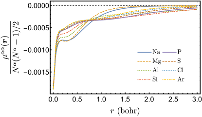
Figure 13: Renormalized $\mu^{\alpha\alpha}(\mathbf{r})$ of the atoms Na to Ar.

Similar to the $\mu^{\alpha\alpha}(\mathbf{r})$ of the second period atoms, the $\mu^{\alpha\alpha}(\mathbf{r})$ of the third period are negative everywhere. The $\mu^{\alpha\alpha}(\mathbf{r})$ of the third period atoms have extra features due to the presence of additional core electrons. The $\mu^{\alpha\alpha}(\mathbf{r})$ of Na and Mg resemble that of Ne. The secondary minimum near the nucleus decreases in magnitude and almost disappears as $\alpha$ $p$-electrons are added from Al to P. For those atoms with $\alpha$ $p$-electrons, there is a less pronounced shoulder at larger $r$.

The $\alpha\alpha$ reduced MB density per $\alpha$ electron is presented for the third period atoms in Figure 14.

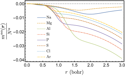
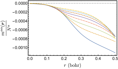
Figure 14: Renormalized $m^{\alpha\alpha}(\mathbf{r})$ of the atoms Na to Ar.

The transition from atoms without valence $p$-electrons to those with them is obvious. The $m^{\alpha\alpha}(\mathbf{r})$ of both Na and Mg have minima in their valence region (similar to Li and Be), whereas the atoms beyond Mg exhibit a shoulder and continue to increase in amplitude. Also similar to the second period, the maximum amplitude of $m^{\alpha\alpha}(\mathbf{r})/N^{\alpha}$ is reached by the atom with only one $p$-electron and the amplitude decreases across the period. Furthermore, the values of $m^{\alpha\alpha}(\mathbf{r})/N^{\alpha}$ converge to a short range of near-zero values close to the nucleus.

Finally, the trend in the total MB between parallel-spin electrons for atoms of the second and third period is illustrated in Figure 15. The actual values can be found in Table I of the supplementary material.

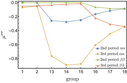
Figure 15: Parallel-spin momentum balance of 2nd and 3rd row atoms.

Fermi correlation, or exchange, is mainly responsible for the shape of $\mu^{\sigma\sigma}(\mathbf{r})$ and the subsequent value of $\mu^{\sigma\sigma}$. In agreement with the findings of Koga,Koga (2002) concerning the the angular separation of electron momenta in atoms, the magnitude of MB is strongly dependent on the $p$-electrons. This is seen with the dramatic decrease in the value of $\mu^{\alpha\alpha}$ from group 2 to 13, and the decrease in $\mu^{\beta\beta}$ seen from group 15 to 16. Interestingly, the minimum value of $\mu^{\alpha\alpha}$ occurs at group 14, rather than group 15 which has the maximum number of unpaired $p$-electrons. Also, it is seen that $\mu^{\beta\beta}$ slightly decreases when $\alpha$ $p$-electrons are added (group 2 to 15), and $\mu^{\alpha\alpha}$ decreases significantly as $\beta$ $p$-electrons are added (group 15 to 17).

The decrease in correlated electron motion, as indicated by the decrease in the magnitude of $\mu^{\alpha\alpha}$, and the actual overall parallel-spin MB ($\mu^{\alpha\alpha}+\mu^{\beta\beta}$), from group 14 to 18, is similar to the decrease seen in opposite-spin MB as the number of valence electrons is increased (10). Due to the calculation of results short of the complete basis set limit, it is somewhat precarious to draw firm conclusions regarding the nature of this decrease for opposite-spin electrons alone. However, $>$99% of parallel-spin MB is due to Fermi correlation which, when considering magnitude, has been modelled precisely. Therefore, the most reasonable explanation for the reduction in correlated motion amongst parallel-spin electrons is the decrease in space available as the electrons are crowded into the valence region. It is expected that the same phenomenon affects the Coulomb correlation of opposite-spin electrons.

As with the opposite-spin MB density analysis, the parallel MB densities and reduced MB densities for $\beta$ electrons are given in the supplementary material due to the similarities in features and trends compared to the $\alpha$ electron densities.

IV.3 Comparing correlation

As previously mentioned, the effect of Fermi correlation on relative momenta is orders of magnitude larger than that of Coulomb correlation between parallel-spin electrons. The effect of Coulomb correlation on opposite-spin electrons is not as small as that on parallel-spin electrons, but there is a difference in magnitude compared to Fermi correlation. There is also a difference in the relative direction of the correlated momenta; Coulomb correlation of opposite-spin electrons favours equimomentum, whereas Fermi correlation favours antimomentum. Figures 16 and 17 compare the reduced MB density for Ne and Ar by scaling the opposite-spin density so that it is similar in magnitude to that of the parallel-spin density, and by reversing the sign.

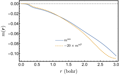
Figure 16: Comparison between $m^{\alpha\alpha}(\mathbf{r})$ and scaled $m^{\alpha\beta}(\mathbf{r})$ of Ne.

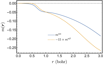
Figure 17: Comparison between $m^{\alpha\alpha}(\mathbf{r})$ and scaled $m^{\alpha\beta}(\mathbf{r})$ of Ar.

It is seen for both Ne and Ar, that while $m^{\alpha\alpha}(\mathbf{r})$ and $m^{\alpha\beta}(\mathbf{r})$ differ in sign, and by an order of magnitude, their shapes are quite similar. Both $m^{\alpha\alpha}(\mathbf{r})$ and $m^{\alpha\beta}(\mathbf{r})$ have minimum amplitude at the nucleus and are relatively flat in the core region. Both increase in magnitude beyond the core and have a slight shoulder as $r$ increases from the core region to the valence region. In the valence region, both increase in amplitude towards the extent of appreciable electron density. At large $r$, the $m(\mathbf{r})$ begin to differ more. For instance, the $m^{\alpha\beta}(\mathbf{r})$ of Ne approaches a maximum near $r=3$, while $m^{\alpha\alpha}(\mathbf{r})$ continues to increase in amplitude. However, the striking similarities of these densities, which are intimately connected to how opposite-spin and parallel-spin electrons avoid each other, cannot be overlooked.

V Conclusions

A more thorough understanding of the correlated motion of electrons (i.e. how electrons avoid each other) is key to unravelling the complexity of the $N$-electron wave function. Such understanding not only allows for the conception of new, more effective, models of electronic structure, but it also increases our basic knowledge of quantum mechanics. The equimomentum, antimomentum and momentum-balance, along with their corresponding densities, provide a means for acheiving such understanding. In addition to being a completely new descriptor of the motion of electrons, MB also serves as a correlated motion detector.

The MB density, $\mu(\mathbf{r})$, povides a measure of the local contribution to momentum-balance in a system of electrons. Due to the dependence of $\mu(\mathbf{r})$ on the probability an electron is found at $\mathbf{r}$, it resembles the one-electron density. The reduced MB density, $m(\mathbf{r})$, removes this dependence and amplifies the more subtle aspects of the local contributions to MB.

The MB, MB density, and reduced MB density can be decomposed into spin contributions. The analysis of the opposite-spin and parallel-spin MB, MB density, and reduced MB density of the atoms He to Ar has revealed significant differences between the correlated motion of opposite-spin and parallel-spin electrons. Fermi correlation, or exchange, causes parallel-spin electrons to move with opposite momentum more than equal momentum. For electrons of opposite spin, Coulomb correlation causes them to move with equal momentum more than opposite momentum. The amount of correlated motion between parallel-spin electrons is strongly dependent on the angular momentum of the electrons present. Whereas, for opposite-spin electrons, the amount of correlated motion is dependent on simply the number of valence electrons present. Also, the effect of Fermi correlation on relative electron momenta is an order of magnitude larger than that of Coulomb correlation.

These new tools, particularly the reduced MB density, have also revealed some subtle similarities between the correlated motion of parallel-spin and opposite-spin electrons. For both, correlated motion, given an electron is present, is a minimum near the nucleus and grows as the distance from the nucleus is increased.

The quantities presented, their derivations, and practical algorithms for their calculation are generalized to abitrary systems of multiple nuclei. Therefore, a natural next step is the investigation of correlated electron motion in molecules. In addition, because MB and the MB densities reveal the presence of electron correlation, they are useful tools for understanding the role of electron correlation in different chemical phenomena (e.g. bond formation/breakage, excited states, dispersion). They also provide a useful tool for assessing the quality of various models of electronic structure. These are just a few of the potential applications of these unique quantum mechanical properties.

Supplementary Material

See supplementary material for recurrence relations for integrals over Gaussian-type basis functions, and additional equations related to the algorithm for the computation of equimomentum, antimomentum, momentum-balance and their corresponding densities. Also, see supplementary material for plots of $\beta\alpha$ and $\beta\beta$ MB densities, as well as numerical values for total atomic MB.

Data Availability

The data that support the findings of this study are available from the corresponding author upon request.

Supplementary Material: Measuring correlated electron motion in atoms with the momentum-balance density

S.I Recurrence relations for $\lambda^{+}$

The equi- and antimomentum, in terms of the spinless 2-RDM, $\Gamma$, are given by,

$$\lambda^{\pm}=\frac{1}{(2\pi)^{3}}\int\Gamma(\mathbf{r}_{1},\mathbf{r}_{2},\mathbf{r}_{1}+\mathbf{q},\mathbf{r}_{2}\mp\mathbf{q})d\mathbf{q}d\mathbf{r}_{1}d\mathbf{r}_{2}.$$ (S1)

Expanding the 2-RDM over a general set of basis functions, $\{\phi_{r}\}$, leads to the alternative expression for the equi- and antimomentum,

$$\lambda^{\pm}=\sum_{rstu}\Gamma_{rstu}\left[rstu\right]_{\lambda^{\pm}},$$ (S2)

where the two-electron integral over four basis functions is given by,

$$\left[rstu\right]_{\lambda^{\pm}}=\frac{1}{(2\pi)^{3}}\int\phi_{r}(\mathbf{r}_{1})\phi_{s}(\mathbf{r}_{1}+\mathbf{q})\\ \times\phi_{t}(\mathbf{r}_{2})\phi_{u}(\mathbf{r}_{2}\mp\mathbf{q})d\mathbf{q}d\mathbf{r}_{1}d\mathbf{r}_{2}.$$ (S3)

In the case of a Gaussian basis set, the fundamental $\lambda^{+}$ integralGill, Johnson, and Pople (1991); Gill (1994) over $s$-type functions with exponents $\alpha$, $\beta$, $\gamma$, $\delta$ and centers $\mathbf{A}$, $\mathbf{B}$, $\mathbf{C}$, $\mathbf{D}$ is given by,

$$\left[\mathbf{0}\mathbf{0}\mathbf{0}\mathbf{0}\right]_{\lambda^{+}}=\frac{\pi^{3/2}e^{-\sigma R^{2}}}{8\left(\alpha\beta\gamma+\beta\gamma\delta+\alpha\beta\delta+\alpha\gamma\delta\right)^{3/2}},$$ (S4)

where

$$\sigma=\frac{\alpha\beta\gamma\delta}{\alpha\beta\gamma+\beta\gamma\delta+\alpha\beta\delta+\alpha\gamma\delta}$$ (S5)

and

$$\mathbf{R}=\mathbf{A}+\mathbf{C}-\mathbf{B}-\mathbf{D}.$$ (S6)

Integrals of higher angular momentum can be constructed using a five-term recurrence relation (RR).Hollett and Gill (2011) The RRs for augmenting the angular momentum of the Gaussians on each centre, $\mathbf{A}$, $\mathbf{B}$, $\mathbf{C}$ and $\mathbf{D}$, in the $i$-direction (where $i=x,y$ or $z$) are given by

$$[(\mathbf{a}+\bm{1}_{i})\mathbf{b}\mathbf{c}\mathbf{d}]_{\lambda^{+}}= -\frac{\sigma}{\alpha}R_{i}[\mathbf{a}\mathbf{b}\mathbf{c}\mathbf{d}]_{\lambda^{+}}$$

$$+a_{i}\frac{\alpha-\sigma}{2\alpha^{2}}[(\mathbf{a}-\bm{1}_{i})\mathbf{b}\mathbf{c}\mathbf{d}]_{\lambda^{+}}$$

$$+b_{i}\frac{\sigma}{2\alpha\beta}[\mathbf{a}(\mathbf{b}-\bm{1}_{i})\mathbf{c}\mathbf{d}]_{\lambda^{+}}$$

$$-c_{i}\frac{\sigma}{2\alpha\gamma}[\mathbf{a}\mathbf{b}(\mathbf{c}-\bm{1}_{i})\mathbf{d}]_{\lambda^{+}}$$

$$+d_{i}\frac{\sigma}{2\alpha\delta}[\mathbf{a}\mathbf{b}\mathbf{c}(\mathbf{d}-\bm{1}_{i})]_{\lambda^{+}},$$ (S7a)

$$[\mathbf{a}(\mathbf{b}+\bm{1}_{i})\mathbf{c}\mathbf{d}]_{\lambda^{+}}= \frac{\sigma}{\beta}R_{i}[\mathbf{a}\mathbf{b}\mathbf{c}\mathbf{d}]_{\lambda^{+}}$$

$$+a_{i}\frac{\sigma}{2\alpha\beta}[(\mathbf{a}-\bm{1}_{i})\mathbf{b}\mathbf{c}\mathbf{d}]_{\lambda^{+}}$$

$$+b_{i}\frac{\beta-\sigma}{2\beta^{2}}[\mathbf{a}(\mathbf{b}-\bm{1}_{i})\mathbf{c}\mathbf{d}]_{\lambda^{+}}$$

$$+c_{i}\frac{\sigma}{2\beta\gamma}[\mathbf{a}\mathbf{b}(\mathbf{c}-\bm{1}_{i})\mathbf{d}]_{\lambda^{+}}$$

$$-d_{i}\frac{\sigma}{2\beta\delta}[\mathbf{a}\mathbf{b}\mathbf{c}(\mathbf{d}-\bm{1}_{i})]_{\lambda^{+}},$$ (S7b)

$$[\mathbf{a}\mathbf{b}(\mathbf{c}+\bm{1}_{i})\mathbf{d}]_{\lambda^{+}}= -\frac{\sigma}{\gamma}R_{i}[\mathbf{a}\mathbf{b}\mathbf{c}\mathbf{d}]_{\lambda^{+}}$$

$$-a_{i}\frac{\sigma}{2\alpha\gamma}[(\mathbf{a}-\bm{1}_{i})\mathbf{b}\mathbf{c}\mathbf{d}]_{\lambda^{+}}$$

$$+b_{i}\frac{\sigma}{2\beta\gamma}[\mathbf{a}(\mathbf{b}-\bm{1}_{i})\mathbf{c}\mathbf{d}]_{\lambda^{+}}$$

$$+c_{i}\frac{\gamma-\sigma}{2\gamma^{2}}[\mathbf{a}\mathbf{b}(\mathbf{c}-\bm{1}_{i})\mathbf{d}]_{\lambda^{+}}$$

$$+d_{i}\frac{\sigma}{2\gamma\delta}[\mathbf{a}\mathbf{b}\mathbf{c}(\mathbf{d}-\bm{1}_{i})]_{\lambda^{+}},$$ (S7c)

$$[\mathbf{a}\mathbf{b}\mathbf{c}(\mathbf{d}+\bm{1}_{i})]_{\lambda^{+}}= \frac{\sigma}{\delta}R_{i}[\mathbf{a}\mathbf{b}\mathbf{c}\mathbf{d}]_{\lambda^{+}}$$

$$+a_{i}\frac{\sigma}{2\alpha\delta}[(\mathbf{a}-\bm{1}_{i})\mathbf{b}\mathbf{c}\mathbf{d}]_{\lambda^{+}}$$

$$-b_{i}\frac{\sigma}{2\beta\delta}[\mathbf{a}(\mathbf{b}-\bm{1}_{i})\mathbf{c}\mathbf{d}]_{\lambda^{+}}$$

$$+c_{i}\frac{\sigma}{2\gamma\delta}[\mathbf{a}\mathbf{b}(\mathbf{c}-\bm{1}_{i})\mathbf{d}]_{\lambda^{+}}$$

$$+d_{i}\frac{\delta-\sigma}{2\delta^{2}}[\mathbf{a}\mathbf{b}\mathbf{c}(\mathbf{d}-\bm{1}_{i})]_{\lambda^{+}},$$ (S7d)

where $\mathbf{a}=(a_{x},a_{y},a_{z})$ is a vector of angular momentum quantum numbers, and $\bm{1}_{i}$ is a unit vector with value 1 in the $i$-direction [e.g. $\bm{1}_{x}=(1,0,0)$].

The momentum-balance (MB) is the difference between the equi- and antimomentum,

$$\mu=\lambda^{+}-\lambda^{-}.$$ (S8)

The effort required to calculate MB is halved by making use of the following identity,

$$[rstu]_{\lambda^{-}}=[rsut]_{\lambda^{+}}.$$ (S9)

Insertion of the 2-RDM expansion (Equation S12) into Equation S8 and use of the identity above (Equation S9) leads to a practical equation for the calculation of MB,

$$\mu=\sum_{rstu}\Gamma_{rstu}\left([rstu]_{\lambda^{+}}-[rsut]_{\lambda^{+}}\right).$$ (S10)

The equi- and antimomentum densities are given by the following equation,

$$\lambda^{\pm}(\mathbf{r})=\frac{1}{(2\pi)^{3}}\int\Gamma(\mathbf{r},\mathbf{r}_{2},\mathbf{r}+\mathbf{q},\mathbf{r}_{2}\mp\mathbf{q})d\mathbf{q}d\mathbf{r}_{2}.$$ (S11)

Similar to equi- and antimomentum, their corresponding densities can also be expanded over a basis set,

$$\lambda^{\pm}(\mathbf{r})=\sum_{rstu}\Gamma_{rstu}\phi_{r}(\mathbf{r})\left[stu\right]_{\lambda^{\pm}},$$ (S12)

where the three-function integral is given by,

$$\left[stu\right]_{\lambda^{\pm}}=\frac{1}{(2\pi)^{3}}\int\phi_{s}(\mathbf{r}+\mathbf{q})\\ \times\phi_{t}(\mathbf{r}_{2})\phi_{u}(\mathbf{r}_{2}\mp\mathbf{q})d\mathbf{q}d\mathbf{r}_{2}.$$ (S13)

If the basis set is comprised of Gaussian-type functions, then the fundamental $\lambda^{+}(\mathbf{r})$ integral is given by,

$$\left[\mathbf{0}\mathbf{0}\mathbf{0}\right]_{\lambda^{+}}=\frac{e^{-\tau P^{2}}}{8\left(\beta\gamma+\beta\delta+\gamma\delta\right)^{3/2}},$$ (S14)

where

$$\tau=\frac{\beta\gamma\delta}{\beta\gamma+\beta\delta+\gamma\delta},$$ (S15)

and

$$\mathbf{P}=\mathbf{r}-\mathbf{B}+\mathbf{C}-\mathbf{D}.$$ (S16)

The integrals over functions of higher angular momentum can be calculated using the following 4-term recurrence relations,

$$[(\mathbf{b}+\bm{1}_{i})\mathbf{c}\mathbf{d}]_{\lambda^{+}}= \frac{\tau}{\beta}P_{i}[\mathbf{b}\mathbf{c}\mathbf{d}]_{\lambda^{+}}$$

$$+b_{i}\frac{\beta-\tau}{2\beta^{2}}[(\mathbf{b}-\bm{1}_{i})\mathbf{c}\mathbf{d}]_{\lambda^{+}}$$

$$+c_{i}\frac{\tau}{2\beta\gamma}[\mathbf{b}(\mathbf{c}-\bm{1}_{i})\mathbf{d}]_{\lambda^{+}}$$

$$-d_{i}\frac{\tau}{2\beta\delta}[\mathbf{b}\mathbf{c}(\mathbf{d}-\bm{1}_{i})]_{\lambda^{+}},$$ (S17a)

$$[\mathbf{b}(\mathbf{c}+\bm{1}_{i})\mathbf{d}]_{\lambda^{+}}= -\frac{\tau}{\gamma}P_{i}[\mathbf{b}\mathbf{c}\mathbf{d}]_{\lambda^{+}}$$

$$+b_{i}\frac{\tau}{2\beta\gamma}[(\mathbf{b}-\bm{1}_{i})\mathbf{c}\mathbf{d}]_{\lambda^{+}}$$

$$+c_{i}\frac{\gamma-\tau}{2\gamma^{2}}[\mathbf{b}(\mathbf{c}-\bm{1}_{i})\mathbf{d}]_{\lambda^{+}}$$

$$+d_{i}\frac{\tau}{2\gamma\delta}[\mathbf{b}\mathbf{c}(\mathbf{d}-\bm{1}_{i})]_{\lambda^{+}},$$ (S17b)

$$[\mathbf{b}\mathbf{c}(\mathbf{d}+\bm{1}_{i})]_{\lambda^{+}}= \frac{\tau}{\delta}P_{i}[\mathbf{b}\mathbf{c}\mathbf{d}]_{\lambda^{+}}$$

$$-b_{i}\frac{\tau}{2\beta\delta}[(\mathbf{b}-\bm{1}_{i})\mathbf{c}\mathbf{d}]_{\lambda^{+}}$$

$$+c_{i}\frac{\tau}{2\gamma\delta}[\mathbf{b}(\mathbf{c}-\bm{1}_{i})\mathbf{d}]_{\lambda^{+}}$$

$$+d_{i}\frac{\delta-\tau}{2\delta^{2}}[\mathbf{b}\mathbf{c}(\mathbf{d}-\bm{1}_{i})]_{\lambda^{+}}.$$ (S17c)

The MB density is calculated as the difference between the equi- and antimomentum densities,

$$\mu(\mathbf{r})=\lambda^{+}(\mathbf{r})-\lambda^{-}(\mathbf{r}).$$ (S18)

To efficiently calculate $\mu(\mathbf{r})$, the following identity is used,

$$[stu]_{\lambda^{-}}=[sut]_{\lambda^{+}}.$$ (S19)

If calculating $\mu(\mathbf{r})$ for numerous values of $\mathbf{r}$, it is desirable to reduce the number of integral evaluations, which can be done with the following expression,

$$\mu(\mathbf{r})=\sum_{rstu}\left(\Gamma_{rstu}-\Gamma_{rsut}\right)\phi_{i}(\mathbf{r})[stu]_{\lambda^{+}}.$$ (S20)

S.II Atomic momentum-balance densities

The $\mu^{\beta\alpha}(\mathbf{r})$, $m^{\beta\alpha}(\mathbf{r})$ and $\mu^{\beta\beta}(\mathbf{r})$, $m^{\beta\beta}(\mathbf{r})$ of the atoms of the first three rows of the periodic table are presented in Figures S1 to S8.

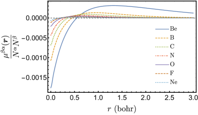
Figure S1: Renormalized $\mu^{\beta\alpha}(\mathbf{r})$ of the atoms Be to Ne.

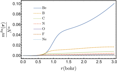
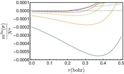
Figure S2: Renormalized $m^{\beta\alpha}(\mathbf{r})$ of the atoms Be to Ne.

Figure S3: Renormalized $\mu^{\beta\alpha}(\mathbf{r})$ of the atoms Na to Ar.

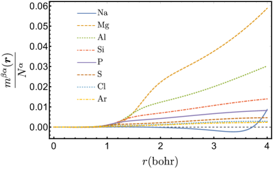
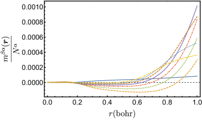
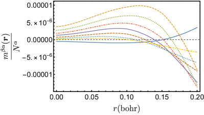
Figure S4: Renormalized $m^{\beta\alpha}(\mathbf{r})$ of the atoms Na to Ar.

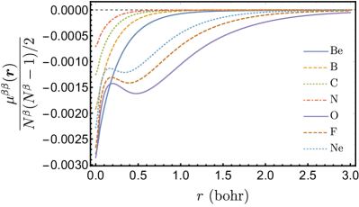
Figure S5: Renormalized $\mu^{\beta\beta}(\mathbf{r})$ of the atoms Be to Ne.

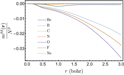
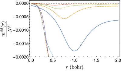
Figure S6: Renormalized $m^{\beta\beta}(\mathbf{r})$ of the atoms Be to Ne.

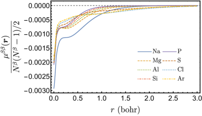
Figure S7: Renormalized $\mu^{\beta\beta}(\mathbf{r})$ of the atoms Na to Ar.

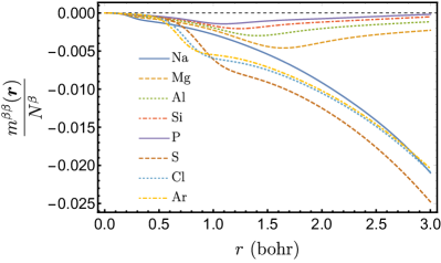
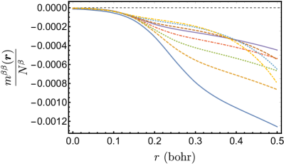
Figure S8: Renormalized $m^{\beta\beta}(\mathbf{r})$ of the atoms Na to Ar.

S.III Atomic momentum-balance

The total opposite-spin and parallel-spin momentum-balance for the atoms He to Ar are reported in Table 1.

Table 1: Spin-resolved and total momentum-balance of the atoms helium to argon

Atom	$\mu^{\alpha\beta}$	$\mu^{\alpha\alpha}$	$\mu^{\beta\beta}$	$\mu$
He	0.00373	0	0	0.00373
Li	0.00107	-0.00001	0	0.00212
Be	0.19320	-0.00240	-0.00240	0.38160
B	0.06497	-0.25768	-0.00077	-0.12851
C	0.02555	-0.27478	-0.00028	-0.22396
N	0.01029	-0.24801	-0.00010	-0.22752
O	0.00770	-0.16412	-0.06507	-0.21380
F	0.00564	-0.11649	-0.08387	-0.18908
Ne	0.00419	-0.08663	-0.08663	-0.16487
Na	0.00095	-0.07077	-0.04902	-0.11788
Mg	0.29053	-0.04855	-0.04855	0.48398
Al	0.13933	-0.76686	-0.03289	-0.52109
Si	0.07348	-0.89145	-0.02315	-0.76764
P	0.03908	-0.87708	-0.01680	-0.81572
S	0.03920	-0.60966	-0.21962	-0.75088
Cl	0.03394	-0.44856	-0.30727	-0.68796
Ar	0.02828	-0.34316	-0.34316	-0.62976

References

- Coulson and Neilson (1961) C. A. Coulson and A. H. Neilson, Proc. Phys. Soc. 78, 831 (1961).
- Lester Jr and Krauss (1966) W. A. Lester Jr and M. Krauss, The Journal of Chemical Physics 44, 207 (1966).
- Coleman (1967) A. J. Coleman, Int. J. Quantum Chem. 1, 457 (1967).
- Banyard and Ellis (1972) K. E. Banyard and D. J. Ellis, Mol. Phys. 24, 1291 (1972).
- Thakkar and Smith Jr. (1977) A. J. Thakkar and V. H. Smith Jr., J. Chem. Phys. 67, 1191 (1977).
- Banyard and Reed (1978) K. E. Banyard and C. E. Reed, J. Phys. B 11, 2957 (1978).
- Sharma and Thakkar (1984) B. S. Sharma and A. J. Thakkar, J. Phys. B 17, 3405 (1984).
- Thakkar, Tripathi, and Smith Jr (1984) A. J. Thakkar, A. N. Tripathi, and V. H. Smith Jr, Phys. Rev. A 29, 1108 (1984).
- Boyd, Sarasola, and Ugalde (1988) R. J. Boyd, C. Sarasola, and J. M. Ugalde, J. Phys. B 21, 2555 (1988).
- Wang, Tripathi, and Smith Jr (1992) J. Wang, A. N. Tripathi, and V. H. Smith Jr, J. Chem. Phys. 97, 9188 (1992).
- Dominguez et al. (1992) L. Dominguez, M. Aguado, C. Sarasola, and J. Ugalde, Journal of Physics B: Atomic, Molecular and Optical Physics 25, 1137 (1992).
- Aguado et al. (1992) M. Aguado, C. Sarasola, L. Dominguez, and J. Ugalde, Journal of Molecular Structure: THEOCHEM 253, 311 (1992).
- Sarasola et al. (1992) C. Sarasola, L. Dominguez, M. Aguado, and J. M. Ugalde, J. Chem. Phys. 96, 6778 (1992).
- Banyard and Sanders (1993) K. E. Banyard and J. Sanders, J. Chem. Phys. 99, 5281 (1993).
- Cann, Boyd, and Thakkar (1993a) N. M. Cann, R. J. Boyd, and A. J. Thakkar, Int. J. Quant. Chem. 48, 1 (1993a).
- Cann, Boyd, and Thakkar (1993b) N. M. Cann, R. J. Boyd, and A. J. Thakkar, J. Chem. Phys. 98, 7132 (1993b).
- Cann, Boyd, and Thakkar (1993c) N. M. Cann, R. J. Boyd, and A. J. Thakkar, Int. J. Quant. Chem. Symp. 27, 33 (1993c).
- Cioslowski and Liu (1996) J. Cioslowski and G. Liu, The Journal of chemical physics 105, 4151 (1996).
- Fradera, Duran, and Mestres (1997) X. Fradera, M. Duran, and J. Mestres, J. Chem. Phys. 107, 3576 (1997).
- Sarsa, Gálvez, and Buendia (1998) A. Sarsa, F. J. Gálvez, and E. Buendia, J. Chem. Phys. 109, 7075 (1998).
- Sarsa, Gálvez, and Buendia (1999) A. Sarsa, F. J. Gálvez, and E. Buendia, J. Chem. Phys. 110, 5721 (1999).
- Fradera, Duran, and Mestres (2000) X. Fradera, M. Duran, and J. Mestres, J. Chem. Phys. 113, 2530 (2000).
- Koga (2001) T. Koga, Chem. Phys. Lett. 350, 135 (2001).
- Koga (2002) T. Koga, Chem. Phys. Lett. 363, 598 (2002).
- Koga and Matsuyama (2003) T. Koga and H. Matsuyama, Chem. Phys. Lett. 375, 565 (2003).
- Gill, O’Neill, and Besley (2003) P. M. W. Gill, D. P. O’Neill, and N. A. Besley, Theor. Chem. Acc. 109, 241 (2003).
- Toulouse, Assaraf, and Umrigar (2007) J. Toulouse, R. Assaraf, and C. J. Umrigar, J. Chem. Phys. 126, 244112 (2007).
- Dumont, Crittenden, and Gill (2007) E. E. Dumont, D. L. Crittenden, and P. M. W. Gill, Phys. Chem. Chem. Phys. 9, 5340 (2007).
- Crittenden, Dumont, and Gill (2007) D. L. Crittenden, E. E. Dumont, and P. M. W. Gill, J. Chem. Phys. 127, 141103 (2007).
- Crittenden and Gill (2007) D. L. Crittenden and P. M. W. Gill, J. Chem. Phys. 127, 014101 (2007).
- Bernard, Crittenden, and Gill (2008) Y. A. Bernard, D. L. Crittenden, and P. M. W. Gill, Phys. Chem. Chem. Phys. 10, 3447 (2008).
- Piris, Lopez, and Ugalde (2008) M. Piris, X. Lopez, and J. M. Ugalde, J. Chem. Phys. 128, 134102 (2008).
- Pearson et al. (2009) J. K. Pearson, P. M. W. Gill, J. M. Ugalde, and R. J. Boyd, Mol. Phys. 107, 1089 (2009).
- Per, Russo, and Snook (2009) M. C. Per, S. P. Russo, and I. K. Snook, J. Chem. Phys. 130, 134103 (2009).
- Hollett and Gill (2011) J. W. Hollett and P. M. W. Gill, Phys. Chem. Chem. Phys. 13, 2972 (2011).
- Loos and Gill (2010) P.-F. Loos and P. M. W. Gill, Phys. Rev. A 81, 052510 (2010).
- Hollett, McKemmish, and Gill (2011) J. W. Hollett, L. K. McKemmish, and P. M. W. Gill, J. Chem. Phys. 134, 224103 (2011).
- Hollett and Gill (2012) J. W. Hollett and P. M. W. Gill, J. Chem. Theory Comput. 8, 1657 (2012).
- Bernard, Loos, and Gill (2013) Y. A. Bernard, P. F. Loos, and P. M. W. Gill, Mol. Phys. 111, 2414 (2013).
- Mercero et al. (2016) J. Mercero, M. Rodríguez-Mayorga, E. Matito, X. Lopez, and J. Ugalde, Canadian Journal of Chemistry 94, 998 (2016), https://doi.org/10.1139/cjc-2016-0203 .
- Hollett and Li (2017) J. W. Hollett and W. Li, The Journal of Physical Chemistry A 121, 8026 (2017).
- Rodríguez-Mayorga et al. (2018) M. Rodríguez-Mayorga, M. Via-Nadal, M. Sola, J. M. Ugalde, X. Lopez, and E. Matito, The Journal of Physical Chemistry A 122, 1916 (2018).
- Rodríguez-Mayorga et al. (2019) M. Rodríguez-Mayorga, E. Ramos-Cordoba, X. Lopez, M. Solà, J. M. Ugalde, and E. Matito, ChemistryOpen 8, 411 (2019).
- Via-Nadal et al. (2019) M. Via-Nadal, M. Rodriguez-Mayorga, E. Ramos-Cordoba, and E. Matito, J. Phys. Chem. Lett. 10, 4032 (2019).
- Gill et al. (2006) P. M. W. Gill, D. L. Crittenden, D. P. O’Neill, and N. A. Besley, Phys. Chem. Chem. Phys. 8, 15 (2006).
- Gill and Chien (2003) P. M. W. Gill and S. Chien, J. Comput. Chem. 24, 732 (2003).
- Cioslowski and Liu (1998) J. Cioslowski and G. Liu, The Journal of chemical physics 109, 8225 (1998).
- Tew, Klopper, and Helgaker (2007) D. P. Tew, W. Klopper, and T. Helgaker, J. Comput. Chem. 28, 1307 (2007).
- Sanders and Banyard (1992) J. Sanders and K. E. Banyard, J. Chem. Phys. 96, 4536 (1992).
- Wang, Kim, and Baerends (2010) J. Wang, K. S. Kim, and E. J. Baerends, The Journal of chemical physics 132, 204102 (2010).
- Cooper and Pounder (1978) I. L. Cooper and C. N. Pounder, Theoretica chimica acta 47, 51 (1978).
- Baerends (2001) E. Baerends, Physical Review Letters 87, 133004 (2001).
- Proud and Pearson (2010) A. J. Proud and J. K. Pearson, J. Chem. Phys. 133, 134113 (2010).
- Proud and Pearson (2012) A. J. Proud and J. K. Pearson, Chem. Phys. Lett. 519–520, 118 (2012).
- Valderrama, Mercero, and Ugalde (2001) E. Valderrama, J. M. Mercero, and J. Ugalde, J. Phys. B 34, 275 (2001).
- Reed and Banyard (1980) C. Reed and K. Banyard, Journal of Physics B: Atomic and Molecular Physics 13, 1519 (1980).
- Ayers, Parr, and Nagy (2002) P. W. Ayers, R. G. Parr, and A. Nagy, International journal of quantum chemistry 90, 309 (2002).
- Anderson, Ayers, and Hernandez (2010) J. S. Anderson, P. W. Ayers, and J. I. R. Hernandez, The Journal of Physical Chemistry A 114, 8884 (2010).
- Bacskay and Nordholm (2017) G. B. Bacskay and S. Nordholm, The Journal of Physical Chemistry A 121, 9330 (2017).
- Huron, Malrieu, and Rancurel (1973) B. Huron, J.-P. Malrieu, and P. Rancurel, J. Chem. Phys. 58, 5745 (1973).
- Giner, Scemama, and Caffarel (2013) E. Giner, A. Scemama, and M. Caffarel, Can. J. Chem. 91, 879 (2013).
- Giner, Scemama, and Caffarel (2015) E. Giner, A. Scemama, and M. Caffarel, J. Chem. Phys. 142, 044115 (2015).
- Garniron et al. (2017) Y. Garniron, A. Scemama, P.-F. Loos, and M. Caffarel, J. Chem. Phys. 147, 034101 (2017).
- Loos et al. (2018) P.-F. Loos, A. Scemama, A. Blondel, Y. Garniron, M. Caffarel, and D. Jacquemin, J. Chem. Theory Comput. 14, 4360 (2018).
- Garniron et al. (2019) Y. Garniron, K. Gasperich, T. Applencourt, A. Benali, A. Ferte, J. Paquier, B. Pradines, R. Assaraf, P. Reinhardt, J. Toulouse, P. Barbaresco, N. Renon, G. David, J. P. Malrieu, M. Veril, M. Caffarel, P. F. Loos, E. Giner, and A. Scemama, J. Chem. Theory Comput. 15, 3591 (2019).
- Dunning Jr. (1989) T. H. Dunning Jr., J. Chem. Phys. 90, 1007 (1989).
- Woon and Dunning Jr. (1994) D. E. Woon and T. H. Dunning Jr., J. Chem. Phys. 100, 2975 (1994).
- Prascher et al. (2011) B. P. Prascher, D. E. Woon, K. A. Peterson, T. H. Dunning, and A. K. Wilson, Theor. Chem. Acc. 128, 69 (2011).
- Feller (1996) D. Feller, J. Comput. Chem. 17, 1571 (1996).
- Schuchardt et al. (2007) K. L. Schuchardt, B. T. Didier, T. Elsethagen, L. Sun, V. Gurumoorthi, J. Chase, J. Li, and T. L. Windus, J. Chem. Inf. Model. 47, 1045 (2007).
- Pritchard et al. (2019) B. P. Pritchard, D. Altarawy, B. Didier, T. D. Gibson, and T. L. Windus, J. Chem. Inf. Model. 59, 4814 (2019).
- Poirier, Hollett, and Warburton (2015) R. A. Poirier, J. W. Hollett, and P. L. Warburton, MUNgauss. Memorial University, Chemistry Department, St. John’s, NL A1B 3X7 (2015), with contributions from A. Alrawashdeh, J.-P. Becker, J. Besaw, S.D. Bungay, F. Colonna, A. El-Sherbiny, T. Gosse, D. Keefe, A. Kelly, D. Nippard, C.C. Pye, D. Reid, K. Saputantri, M. Shaw, M. Staveley, O. Stueker, Y. Wang, and J. Xidos.
- Gill, Johnson, and Pople (1993) P. M. W. Gill, B. G. Johnson, and J. A. Pople, Chem. Phys. Lett. 209, 506 (1993).
- Gill, Johnson, and Pople (1991) P. M. W. Gill, B. G. Johnson, and J. A. Pople, Int. J. Quantum Chem. 40, 745 (1991).
- Gill (1994) P. M. W. Gill, Adv. Quantum Chem. 25, 141 (1994).