acronymindexonlyfirsttrue \newabbreviationqsarQSARQuantitative Structure-Activity-Relationship \newabbreviationnlpNLPNatural Language Processing \newabbreviationecfpECFPExtended-Connectivity Fingerprint \newabbreviationbertBERTBidirectional Encoder Representations from Transformers \newabbreviationsmilesSMILESSimplified Molecular Input Line Entry System \newabbreviationsvmSVMSupport Vector Machine
Molecular representation learning with language models and domain-relevant auxiliary tasks
Abstract
We apply a Transformer architecture, specifically BERT, to learn flexible and high quality molecular representations for drug discovery problems, and study the impact of using different combinations of self-supervised tasks for pre-training. Our results on established Virtual Screening and QSAR benchmarks show that: i) The selection of appropriate self-supervised task(s) for pre-training has a significant impact on performance in subsequent downstream tasks such as Virtual Screening. ii) Using auxiliary tasks with more domain relevance for Chemistry, such as learning to predict calculated molecular properties, increases the fidelity of our learnt representations. iii) Finally, we show that molecular representations learnt by our model ‘MolBert’ improve upon the current state of the art on the benchmark datasets.
1 Introduction
Molecular representations underpin predictive, generative and analytical tasks in drug discovery [1]. The choice of a suitable representation can drastically impact the efficiency of discovering a novel drug candidate. For instance, applications such as Virtual Screening and modeling rely on the availability of effective molecular representations [2].
Language models have been applied to text-based molecular representations such as [3]. They show impressive performance across a range of domain applications including molecular property [4, 5] and reaction prediction problems [6, 7], as well as generative tasks [8]. Numerous strategies have been explored to encourage learning of high quality representations with language models including input reconstruction [9, 10, 11], whereby a model learns to predict masked or corrupted tokens; and input translation [5, 12], where the goal is to translate the input to another modality or representation. Further improvements have been made by incorporating calculated molecular properties into the representation, either by concatenating with the learnt representations [13], or through devising pre-training schemes [14]. Finally, a range of model architectures have been explored including autoencoders [5], RNNs [9] and transformers [10, 11].
Aside from the modal limitations of representing molecules as strings, a drawback to learning from text-based molecular representations is introduced by the ambiguity of linearizing the molecular graph [15]. In the case of , many valid sequences may represent the same molecule depending on the traversal path of the molecular graph. This ambiguity has led to the development of canonicalization algorithms [16, 17] which, while practical, introduce artifacts to linearized such that a language model may be distracted by the rules of canonicalization. Previous works have shown the benefits of learning using permutations of [18].
In this work, we evaluate the application of the widely used [19] architecture for the generation of molecular representations. We explore the impact of employing a range of domain-relevant auxiliary tasks during pre-training and evaluate the produced learnt representations on downstream Virtual Screening and benchmarks. Code and pre-trained models are available at https://github.com/BenevolentAI/MolBERT.
2 MolBert
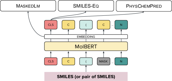
MolBert, as depicted in Figure 1, is a bidirectional language model that uses the architecture [19]. To understand the impact of pre-training with different domain-relevant tasks on downstream applications, we experiment with the following set of self-supervised tasks:
- Masked language modeling (MaskedLM):
-
The canonical task proposed by BERT, whereby the model is trained to predict the true identity of masked tokens. The task is optimized using the cross-entropy loss between the sequence output and the masked tokens of the input.
- SMILES equivalence (SMILES-Eq):
-
Given an input of two SMILES where the second is, with equal probability, either randomly sampled from the training set or a synonymous permutation of the first SMILES, the task is to predict whether the two inputs represent the same molecule. This is a binary classification task, which may be traditionally solved by comparing the canonicalized molecular graphs of the inputs. It is optimized using the cross-entropy loss.
- Calculated molecular descriptor prediction (PhysChemPred):
-
Using RDKit [20] we are able to calculate a simple set of real-valued descriptors of chemical characteristics and composite models of physicochemical properties for each molecule (see Appendix C). The goal of this task is to predict the normalized [21] set of descriptors for each molecule. The task is optimized using the mean squared error over all predicted values.
The final loss is given by the arithmetic mean of all individual task losses.
Fine-tuning
The representations learnt after pre-training MolBert may be applied to downstream tasks in several manners. Here we explore: i) using representations directly for similarity search, ii) training a downstream model; in this case, following Winter et al. [5], we use a , and finally iii), following [19], we add an explicit downstream task head in the form of a newly initialized network which is then optimized.
Evaluation methodology
We evaluate MolBert on two downstream applications: Virtual Screening and . In Virtual Screening
we are typically interested in selecting from a pool of candidate compounds the ones that best satisfy a property of interest, such as the likelihood of binding to a particular drug target. Alternatively, in we are interested in learning to predict a given molecular property, such as the binding affinity to a target of interest. We evaluate MolBert when used directly and when specialized for downstream applications using two established benchmarks:
- Virtual Screening:
-
we use the filtered virtual screening subset (version 1.2) from the RDKit benchmarking platform [22, 23]. The benchmark is made up of datasets, each corresponding to an individual protein target. Each dataset consists of a small number of active molecules amongst a larger number of target specific decoys. The benchmark measures how well-suited molecular representations are to retrieving active compounds from the pool, given a fixed number of query molecules () – for details see Riniker and Landrum [22].
Retrieval is performed according to the cosine distance between MolBert embeddings. Following Riniker and Landrum [22], we report results using: i) the Area Under the Curve of the Receiver Operating Characteristic (AUROC) and ii) the Boltzmann-Enhanced Discrimination of ROC (BEDROC, ) – a widely used early enrichment metric that assigns higher weight to the first of molecules retrieved from the pool according to the Boltzmann distribution [24].
- :
-
we use a subset of the MoleculeNet benchmark suite [25], which consists of datasets of varying size for a range of problems. Specifically we report regression results for the ESOL, FreeSolv and Lipophilicity datasets, as well as classification results for the BACE, BBBP and HIV datasets. Since MoleculeNet does not provide explicit training, validation and test folds for all datasets, we use folds provided by ChemBench [26] to present reproducible results.
3 Experimental Evaluation
In this section, we first present an ablation on MolBert using the different pre-training tasks using the Virtual Screening datasets, then report our results in the Virtual Screening and benchmarks.
| w/ permutation | w/o permutation | |||||
|---|---|---|---|---|---|---|
| MaskedLM | PhysChemPred | SMILES-Eq | AUROC | BEDROC20 | AUROC | BEDROC20 |
| ✓ | ✓ | ✓ | ||||
| ✓ | ✓ | ✗ | ||||
| ✓ | ✗ | ✓ | ||||
| ✗ | ✓ | ✓ | ||||
| ✓ | ✗ | ✗ | ||||
| ✗ | ✓ | ✗ | ||||
| ✗ | ✗ | ✓ | ||||
| AUROC | BEDROC20 | |
|---|---|---|
| MolBert(100 epochs) | ||
| CDDD | ||
| RDKit descriptors | ||
| ECFC4 |
Pre-training dataset: All models are pre-trained using the GuacaMol benchmark dataset [27] consisting of 1.6M compounds curated from ChEMBL [28]. We use the training and validation splits which consist of 80% and 5% of the data, respectively.
Models: MolBert models are implemented using the Hugging Face transformers library [29], and use the BERT-Base architecture (12 attention heads, 12 layers, 768 dimensional hidden layer, 85M parameters). We use the Adam optimizer [30] with a learning rate of , and train for 20 epochs, except for the final model, which we train for 100 epochs. The average pre-training time for MolBert was 40 hours using 2 GPUs and 16 CPUs.
Fine-tuning: All experiments use the same base model, the best model from the ablation trained for 100 epochs. To ease reproducibility we use the parameters published in Winter et al. [5] (, RBF kernel) and all fine-tuning networks are a single linear layer attached to the pooled output. To generate molecular embeddings we use the pooled output, except where MaskedLM is the only task used for pre-training, in which case we use the average of the sequence output, since the pooled output has no dependent tasks.
MolBert is trained using a fixed vocabulary of tokens and a sequence length of characters. In line with [19], all tasks are trained by masking 15% of the tokenized input. To support the use of arbitrary length input SMILES at inference time, we use relative positional embeddings as described by Dai et al. [31].
| Regression Datasets: RMSE | |||||
|---|---|---|---|---|---|
| RDKit (norm) | ECFC4 | CDDD | MolBert | MolBert (finetune) | |
| ESOL | |||||
| FreeSolv | |||||
| Lipop | |||||
| Classification Dataset: AUROC | |||||
| RDKit (norm) | ECFC4 | CDDD | MolBERT | MolBERT (finetune) | |
| BACE | |||||
| BBBP | |||||
| HIV | |||||
Results
Ablation study: We first analyze the utility of using different combinations of tasks for pre-training. From Table 2, the main observations are that: i) The PhysChemPred task has the highest impact on the performance metrics, with an average BEDROC20 of when using the PhysChemPred task alone (with and without permutations) versus for the MaskedLM alone. ii) Although the best performing model is trained on both the PhysChemPred and MaskedLM, the additive gain from the MaskedLM task is relatively minor; on average for the BEDROC20 metric. iii) The addition of the SMILES-Eq task slightly but consistently decreases performance.
Given the effectiveness of pre-training with the PhysChemPred task, we explored the impact of grouping the calculated descriptors into disjoint related subsets. Table A5 shows that, although using All the descriptors achieves the best overall result, the surface properties of a molecule provide a very competitive supervision task using only 25% of the descriptors.
Virtual Screening: Table 2 compares the performance of MolBert when trained for 100 epochs with the best performing auxiliary task combination, with three baseline methods. i) CDDD [5], a neural model that achieves the current state-of-the-art results for this benchmark. ii) The RDKit calculated physicochemical descriptors [20] used for the PhysChemPred task during pre-training. iii) Extended Connectivity Fingerprints with a diamater of 4 (ECFC4), one of the most commonly used descriptors in drug discovery. Our results show that MolBert outperforms all other descriptors both in terms of overall classification and early enrichment. A detailed breakdown of per-dataset results is given in Figure A1 for the BEDROC20 and AUROC, respectively. Finally, upon closer investigation as to the benefit of input permutation and calculated molecular property prediction, we observed that these strategies enable MolBert to organize the learnt embeddings. More concretely, pre-training with the PhysChemPred task and input permutation leads to models which on average assign a lower pairwise similarity to non-identical compounds; see Appendix B.
: To further evaluate the usefulness of MolBert embeddings, we build models for datasets from MoleculeNet [25] and include models built using CDDD [5], ECFC4 [32] and the normalized RDKit calculated physicochemical descriptors [20] as baselines. As described in Section 2, we train an (implemented using sklearn [33]) using each molecular representation, and compare against fine-tuning MolBert.
From the results in Table 3, we see that neural models substantially outperform traditional molecular representations (RDKIT and ECFC4). Furthermore, finetuned MolBert models achieve the best performance in all of the six benchmark datasets. We also observe that MolBert representations combined with a SVM outperform the other descriptors on three of the six tasks.
4 Conclusions
We have introduced MolBert, a language model for learning molecular embeddings using . We investigated the impact of pre-training with domain-relevant auxiliary tasks and found that the choice of self supervision task significantly impacts the performance on downstream tasks. Nevertheless, with the right set of tasks MolBert achieves state-of-the-art performance on established Virtual Screening and benchmarks. We leave to future work the exploration of how to use MolBert for learning representations of other entities such as proteins [34, 35, 36], along with further developments in our learning strategies [37].
References
- David et al. [2020] Laurianne David, Amol Thakkar, Rocío Mercado, and Ola Engkvist. Molecular representations in AI-driven drug discovery: a review and practical guide. Journal of Cheminformatics, 12(1):1–22, 2020.
- Vamathevan et al. [2019] Jessica Vamathevan, Dominic Clark, Paul Czodrowski, Ian Dunham, Edgardo Ferran, George Lee, Bin Li, Anant Madabhushi, Parantu Shah, Michaela Spitzer, and Shanrong Zhao. Applications of machine learning in drug discovery and development. Nature Reviews Drug Discovery, 18(6):463–477, 2019.
- Weininger [1988] David Weininger. Smiles, a chemical language and information system. 1. introduction to methodology and encoding rules. Journal of chemical information and computer sciences, 28(1):31–36, 1988.
- Jastrzębski et al. [2016] Stanisław Jastrzębski, Damian Leśniak, and Wojciech Marian Czarnecki. Learning to SMILE (S). arXiv preprint arXiv:1602.06289, 2016.
- Winter et al. [2019] Robin Winter, Floriane Montanari, Frank Noé, and Djork-Arné Clevert. Learning continuous and data-driven molecular descriptors by translating equivalent chemical representations. Chemical Science, 10(6):1692–1701, 2019.
- Liu et al. [2017] Bowen Liu, Bharath Ramsundar, Prasad Kawthekar, Jade Shi, Joseph Gomes, Quang Luu Nguyen, Stephen Ho, Jack Sloane, Paul Wender, and Vijay Pande. Retrosynthetic reaction prediction using neural sequence-to-sequence models. ACS Central Science, 3(10):1103–1113, 2017.
- Schwaller et al. [2019] Philippe Schwaller, Teodoro Laino, Théophile Gaudin, Peter Bolgar, Christopher A Hunter, Costas Bekas, and Alpha A Lee. Molecular transformer: A model for uncertainty-calibrated chemical reaction prediction. ACS Central Science, 5(9):1572–1583, 2019.
- Segler et al. [2018] Marwin HS Segler, Thierry Kogej, Christian Tyrchan, and Mark P Waller. Generating focused molecule libraries for drug discovery with recurrent neural networks. ACS Central Science, 4(1):120–131, 2018.
- Li and Fourches [2020] Xinhao Li and Denis Fourches. Inductive Transfer Learning for Molecular Activity Prediction: Next-Gen QSAR Models with MolPMoFiT. Journal of Cheminformatics, 12(27):1–15, 2020.
- Łukasz Maziarka et al. [2020] Łukasz Maziarka, Tomasz Danel, Sławomir Mucha, Krzysztof Rataj, Jacek Tabor, and Stanisław Jastrzębski. Molecule Attention Transformer. arXiv preprint arXiv:2002.08264, 2020.
- Wang et al. [2019] Sheng Wang, Yuzhi Guo, Yuhong Wang, Hongmao Sun, and Junzhou Huang. Smiles-bert: Large scale unsupervised pre-training for molecular property prediction. In Proceedings of the 10th ACM International Conference on Bioinformatics, Computational Biology and Health Informatics, page 429–436, 2019. doi: 10.1145/3307339.3342186.
- Morris et al. [2020] Paul Morris, Rachel St. Clair, William Edward Hahn, and Elan Barenholtz. Predicting binding from screening assays with transformer network embeddings. Journal of Chemical Information and Modeling, 60(9):4191–4199, 2020.
- Yang et al. [2019a] Kevin Yang, Kyle Swanson, Wengong Jin, Connor Coley, Philipp Eiden, Hua Gao, Angel Guzman-Perez, Timothy Hopper, Brian Kelley, Miriam Mathea, Andrew Palmer, Volker Settels, Tommi Jaakkola, Klavs Jensen, and Regina Barzilay. Analyzing learned molecular representations for property prediction. Journal of Chemical Information and Modeling, 59(8):3370–3388, 2019a.
- Goh et al. [2018] Garrett B. Goh, Charles Siegel, Abhinav Vishnu, and Nathan Hodas. Using Rule-Based Labels for Weak Supervised Learning: A ChemNet for Transferable Chemical Property Prediction. In Proceedings of the 24th ACM SIGKDD International Conference on Knowledge Discovery & Data Mining, page 302–310, 2018. doi: 10.1145/3219819.3219838.
- Randić [1977] Milan Randić. On canonical numbering of atoms in a molecule and graph isomorphism. Journal of Chemical Information and Computer Sciences, 17(3):171–180, 1977.
- Weisfeiler and Lehman [1968] B. Weisfeiler and A. A. Lehman. A reduction of a graph to a canonical form and an algebra arising during this reduction. Nauchno-Technicheskaya Informatsia, 2(9), 1968.
- Schneider et al. [2015] Nadine Schneider, Roger A. Sayle, and Gregory A. Landrum. Get your atoms in order—an open-source implementation of a novel and robust molecular canonicalization algorithm. Journal of Chemical Information and Modeling, 55(10):2111–2120, 2015.
- Bjerrum and Sattarov [2018] Esben Jannik Bjerrum and Boris Sattarov. Improving Chemical Autoencoder Latent Space and Molecular De Novo Generation Diversity with Heteroencoders. Biomolecules, 8(4):131, 2018.
- Devlin et al. [2018] Jacob Devlin, Ming-Wei Chang, Kenton Lee, and Kristina Toutanova. BERT: pre-training of deep bidirectional transformers for language understanding. arXiv preprint arXiv:1810.04805, 2018.
- Landrum [2020] G. A. Landrum. RDKit: Open-Source Cheminformatics Software, 2020. URL http://www.rdkit.org.
- Yang et al. [2019b] Kevin Yang, Kyle Swanson, Wengong Jin, Connor Coley, Philipp Eiden, Hua Gao, Angel Guzman-Perez, Timothy Hopper, Brian Kelley, Miriam Mathea, Andrew Palmer, Volker Settels, Tommi Jaakkola, Klavs Jensen, and Regina Barzilay. Analyzing learned molecular representations for property prediction. Journal of Chemical Information and Modeling, 59(8):3370–3388, 2019b.
- Riniker and Landrum [2013] Sereina Riniker and Gregory A Landrum. Open-source platform to benchmark fingerprints for ligand-based virtual screening. Journal of Cheminformatics, 5(1):26, 2013.
- Riniker et al. [2013] Sereina Riniker, Nikolas Fechner, and Gregory A Landrum. Heterogeneous classifier fusion for ligand-based virtual screening: or, how decision making by committee can be a good thing. Journal of Chemical Information and Modeling, 53(11):2829–2836, 2013.
- Truchon and Bayly [2007] Jean-François Truchon and Christopher I Bayly. Evaluating virtual screening methods: good and bad metrics for the “early recognition” problem. Journal of Chemical Information and Modeling, 47(2):488–508, 2007.
- Wu et al. [2018] Zhenqin Wu, Bharath Ramsundar, Evan N Feinberg, Joseph Gomes, Caleb Geniesse, Aneesh S Pappu, Karl Leswing, and Vijay Pande. Moleculenet: a benchmark for molecular machine learning. Chemical Science, 9(2):513–530, 2018.
- Wanxiang [2020] Shen Wanxiang. ChemBench: The molecule benchmarks and MolMapNet datasets, 2020. URL https://github.com/shenwanxiang/ChemBench.
- Brown et al. [2019] Nathan Brown, Marco Fiscato, Marwin H.S. Segler, and Alain C. Vaucher. GuacaMol: Benchmarking Models for de Novo Molecular Design. Journal of Chemical Information and Modeling, 59(3):1096–1108, 2019.
- Gaulton et al. [2017] Anna Gaulton, Anne Hersey, Michał Nowotka, A. Patrícia Bento, Jon Chambers, David Mendez, Prudence Mutowo, Francis Atkinson, Louisa J. Bellis, Elena Cibrián-Uhalte, Mark Davies, Nathan Dedman, Anneli Karlsson, María Paula Magariños, John P. Overington, George Papadatos, Ines Smit, and Andrew R. Leach. The ChEMBL database in 2017. Nucleic Acids Research, 45(D1):D945–D954, 2017.
- Wolf et al. [2019] Thomas Wolf, Lysandre Debut, Victor Sanh, Julien Chaumond, Clement Delangue, Anthony Moi, Pierric Cistac, Tim Rault, Rémi Louf, Morgan Funtowicz, Joe Davison, Sam Shleifer, Patrick von Platen, Clara Ma, Yacine Jernite, Julien Plu, Canwen Xu, Teven Le Scao, Sylvain Gugger, Mariama Drame, Quentin Lhoest, and Alexander M. Rush. HuggingFace’s Transformers: State-of-the-art Natural Language Processing. arXiv preprint arXiv:1910.03771, 2019.
- Kingma and Ba [2014] Diederik P Kingma and Jimmy Ba. Adam: A Method for Stochastic Optimization. arXiv preprint arXiv:1412.6980, 2014.
- Dai et al. [2019] Zihang Dai, Zhilin Yang, Yiming Yang, Jaime G. Carbonell, Quoc V. Le, and Ruslan Salakhutdinov. Transformer-xl: Attentive language models beyond a fixed-length context. arXiv preprint arXiv:1901.02860, 2019.
- Rogers and Hahn [2010] David Rogers and Mathew Hahn. Extended-connectivity fingerprints. Journal of Chemical Information and Modeling, 50(5):742–754, 2010.
- Pedregosa et al. [2011] F. Pedregosa, G. Varoquaux, A. Gramfort, V. Michel, B. Thirion, O. Grisel, M. Blondel, P. Prettenhofer, R. Weiss, V. Dubourg, J. Vanderplas, A. Passos, D. Cournapeau, M. Brucher, M. Perrot, and E. Duchesnay. Scikit-learn: Machine learning in Python. Journal of Machine Learning Research, 12:2825–2830, 2011.
- Simonovsky and Meyers [2020] Martin Simonovsky and Joshua Meyers. Deeplytough: Learning structural comparison of protein binding sites. Journal of Chemical Information and Modeling, 60(4):2356–2366, 2020.
- Alley et al. [2019] Ethan C Alley, Grigory Khimulya, Surojit Biswas, Mohammed AlQuraishi, and George M Church. Unified rational protein engineering with sequence-based deep representation learning. Nature Methods, 16(12):1315–1322, 2019.
- Kim et al. [2020] Paul Kim, Robin Winter, and Djork-Arné Clevert. Deep protein-ligand binding prediction using unsupervised learned representations. ChemRxiv, 2020. doi: 10.26434/chemrxiv.11523117.v1.
- Hu et al. [2019] Weihua Hu, Bowen Liu, Joseph Gomes, Marinka Zitnik, Percy Liang, Vijay S. Pande, and Jure Leskovec. Strategies for Pre-training Graph Neural Networks. arXiv preprint arXiv:1905.12265, 2019.
- Maaten and Hinton [2008] Laurens van der Maaten and Geoffrey Hinton. Visualizing data using t-SNE. Journal of Machine Learning Research, 9(Nov):2579–2605, 2008.
Appendix
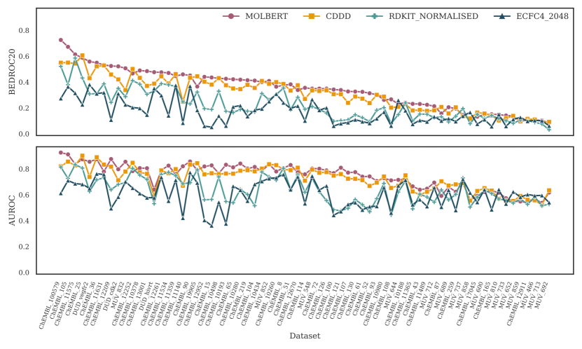
Appendix A Virtual Screening benchmark: performance per target
Figure A1 shows results for MolBert and other baseline methods on the individual Virtual Screening datasets listed in [22]. The datasets are sorted based on the BEDROC20 enrichment metric. We observe that MolBert displays superior performance for 45 of 69 targets and performs competitively in all other cases.
Appendix B Auxiliary task induced biases in MolBert models
| Seed Molecule | Permutations | |
|---|---|---|
| \cellcolorcolor-4A9995!95 Palbociclib |
![[Uncaptioned image]](/html/2011.13230/assets/x3.png)
|
|
| C1(NC2=NC=C(N3CCNCC3)C=C2)=NC=C2C(C)=C(C(C)=O)C(=O)N(C3CCCC3)C2=N1 | C1(NC2=NC=C(N3CCNCC3)C=C2)=NC=C2C(C)=C(C(C)=O)C(=O)N(C3CCCC3)C2=N1 | |
| C1CCC(N2C3=NC(NC4=NC=C(N5CCNCC5)C=C4)=NC=C3C(C)=C(C(=O)C)C2=O)C1 | ||
| C1(C)=C(C(C)=O)C(=O)N(C2CCCC2)C2=NC(NC3=NC=C(N4CCNCC4)C=C3)=NC=C12 | ||
| C1C(N2C3=NC(NC4=NC=C(N5CCNCC5)C=C4)=NC=C3C(C)=C(C(=O)C)C2=O)CCC1 | ||
| N1=C(NC2=NC=C3C(C)=C(C(=O)C)C(=O)N(C4CCCC4)C3=N2)C=CC(N2CCNCC2)=C1 | ||
| C1=CC(N2CCNCC2)=CN=C1NC1=NC=C2C(C)=C(C(=O)C)C(=O)N(C3CCCC3)C2=N1 | ||
| C1NCCN(C2=CN=C(NC3=NC=C4C(C)=C(C(C)=O)C(=O)N(C5CCCC5)C4=N3)C=C2)C1 | ||
| C1CCC(N2C3=NC(NC4=NC=C(N5CCNCC5)C=C4)=NC=C3C(C)=C(C(C)=O)C2=O)C1 | ||
| C1CN(C2=CN=C(NC3=NC=C4C(=N3)N(C3CCCC3)C(=O)C(C(=O)C)=C4C)C=C2)CCN1 | ||
| N1(C2=CN=C(NC3=NC=C4C(=N3)N(C3CCCC3)C(=O)C(C(C)=O)=C4C)C=C2)CCNCC1 | ||
| \cellcolorcolor-A65B73!95 Seliciclib |
![[Uncaptioned image]](/html/2011.13230/assets/x4.png)
|
|
| CC[C@H](CO)NC1=NC(NCC2=CC=CC=C2)=C2C(=N1)N(C(C)C)C=N2 | C(NC1=C2C(=NC(N[C@H](CC)CO)=N1)N(C(C)C)C=N2)C1=CC=CC=C1 | |
| C(NC1=C2N=CN(C(C)C)C2=NC(N[C@@H](CO)CC)=N1)C1=CC=CC=C1 | ||
| C1=CC=C(CNC2=C3C(=NC(N[C@@H](CO)CC)=N2)N(C(C)C)C=N3)C=C1 | ||
| CC(C)N1C=NC2=C(NCC3=CC=CC=C3)N=C(N[C@@H](CO)CC)N=C12 | ||
| C1=CC(CNC2=C3N=CN(C(C)C)C3=NC(N[C@H](CC)CO)=N2)=CC=C1 | ||
| N1(C(C)C)C2=NC(N[C@@H](CO)CC)=NC(NCC3=CC=CC=C3)=C2N=C1 | ||
| CC(C)N1C2=NC(N[C@@H](CO)CC)=NC(NCC3=CC=CC=C3)=C2N=C1 | ||
| C12=NC(N[C@H](CC)CO)=NC(NCC3=CC=CC=C3)=C1N=CN2C(C)C | ||
| [C@H ](CO)(CC)NC1=NC(NCC2=CC=CC=C2)=C2C(=N1)N(C(C)C)C=N2 | ||
| C1=C(CNC2=C3N=CN(C(C)C)C3=NC(N[C@@H](CO)CC)=N2)C=CC=C1 | ||
| \cellcolorcolor-EB9706!95 Venetoclax |
![[Uncaptioned image]](/html/2011.13230/assets/x5.png)
|
|
| CC1(C)CCC(CN2CCN(C3=CC(OC4=CN=C5C(=C4)C=CN5)=C(C(=O)NS(=O)(=O)C4=CC([N+](=O)[O-])=C(NCC5CCOCC5)C=C4)C=C3)CC2)=C(C2=CC=C(Cl)C=C2)C1 | C1CN(CC2=C(C3=CC=C(Cl)C=C3)CC(C)(C)CC2)CCN1C1=CC(OC2=CN=C3C(=C2)C=CN3)=C(C(NS(C2=CC([N+]([O-])=O)=C(NCC3CCOCC3)C=C2)(=O)=O)=O)C=C1 | |
| C1=CC(C(=O)NS(=O)(=O)C2=CC([N+](=O)[O-])=C(NCC3CCOCC3)C=C2)=C(OC2=CN=C3C(=C2)C=CN3)C=C1N1CCN(CC2=C(C3=CC=C(Cl)C=C3)CC(C)(C)CC2)CC1 | ||
| [N+ ](=O)(C1=C(NCC2CCOCC2)C=CC(S(NC(=O)C2=CC=C(N3CCN(CC4=C(C5=CC=C(Cl)C=C5)CC(C)(C)CC4)CC3)C=C2OC2=CN=C3C(=C2)C=CN3)(=O)=O)=C1)[O-] | ||
| C1(C2=CC=C(Cl)C=C2)=C(CN2CCN(C3=CC(OC4=CN=C5NC=CC5=C4)=C(C(NS(=O)(C4=CC([N+]([O-])=O)=C(NCC5CCOCC5)C=C4)=O)=O)C=C3)CC2)CCC(C)(C)C1 | ||
| [O- ][N+ ](=O)C1=C(NCC2CCOCC2)C=CC(S(=O)(NC(=O)C2=CC=C(N3CCN(CC4=C(C5=CC=C(Cl)C=C5)CC(C)(C)CC4)CC3)C=C2OC2=CN=C3NC=CC3=C2)=O)=C1 | ||
| C1(OC2=CN=C3C(=C2)C=CN3)=CC(N2CCN(CC3=C(C4=CC=C(Cl)C=C4)CC(C)(C)CC3)CC2)=CC=C1C(NS(C1=CC([N+](=O)[O-])=C(NCC2CCOCC2)C=C1)(=O)=O)=O | ||
| C1(C2=C(CN3CCN(C4=CC(OC5=CN=C6C(=C5)C=CN6)=C(C(=O)NS(=O)(C5=CC([N+](=O)[O-])=C(NCC6CCOCC6)C=C5)=O)C=C4)CC3)CCC(C)(C)C2)=CC=C(Cl)C=C1 | ||
| C1(N2CCN(CC3=C(C4=CC=C(Cl)C=C4)CC(C)(C)CC3)CC2)=CC(OC2=CN=C3C(=C2)C=CN3)=C(C(=O)NS(C2=CC([N+]([O-])=O)=C(NCC3CCOCC3)C=C2)(=O)=O)C=C1 | ||
| C1C(CNC2=C([N+](=O)[O-])C=C(S(=O)(NC(=O)C3=CC=C(N4CCN(CC5=C(C6=CC=C(Cl)C=C6)CC(C)(C)CC5)CC4)C=C3OC3=CN=C4NC=CC4=C3)=O)C=C2)CCOC1 | ||
| C12=CC(OC3=CC(N4CCN(CC5=C(C6=CC=C(Cl)C=C6)CC(C)(C)CC5)CC4)=CC=C3C(NS(=O)(=O)C3=CC([N+]([O-])=O)=C(NCC4CCOCC4)C=C3)=O)=CN=C1NC=C2 | ||
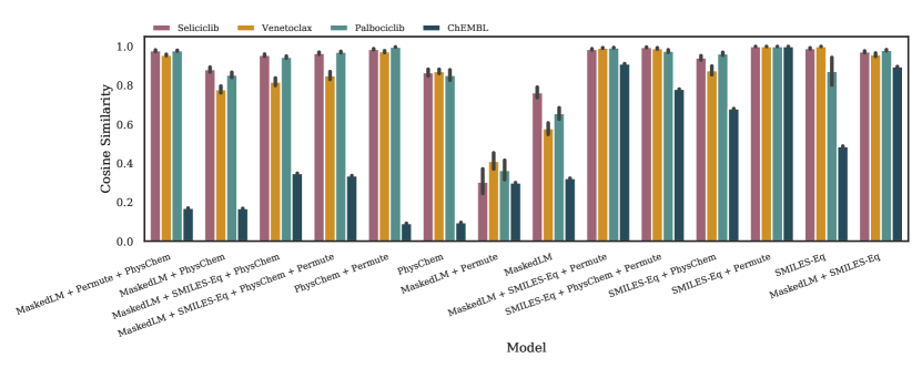
To understand the types of inductive biases introduced by the different auxiliary tasks used in pre-training, we explore the difference in behaviour of the resulting learnt representations.
Appendix B lists three well-studied compounds. We sample ten random permutations of each, along with 1000 randomly selected molecules from ChEMBL, and use this data to compare the distributions of pairwise cosine similarities of the representations learnt with each task combination in Table 2.
Since the benchmark is a nearest neighbor retrieval task, we aim to understand whether learning to finely disambiguate between molecules correlates with benchmark performance. We hypothesize that models that achieve high average pairwise similarity between permutations of the same molecule and a low average pairwise similarity between random molecules achieve improved benchmark performance.
| MaskedLM + Permute + PhysChem | PhysChem + Permute | MaskedLM + SMILES-Eq + PhysChem + Permute |
![[Uncaptioned image]](/html/2011.13230/assets/x7.png) |
![[Uncaptioned image]](/html/2011.13230/assets/x8.png) |
![[Uncaptioned image]](/html/2011.13230/assets/x9.png) |
| MaskedLM | MaskedLM + Permute |
![[Uncaptioned image]](/html/2011.13230/assets/x10.png) |
![[Uncaptioned image]](/html/2011.13230/assets/x11.png) |
| SMILES-Eq + Permute | MaskedLM + SMILES-Eq + Permute |
![[Uncaptioned image]](/html/2011.13230/assets/x12.png) |
![[Uncaptioned image]](/html/2011.13230/assets/x13.png) |
Figure A2 gives the results of our analysis where we observe three broad behaviours: First, MolBert models that were pre-trained on task combinations including the physicochemical property prediction (PhysChemPred) task successfully assign high similarities to permutations of the same molecule, while assigning low average similarity between randomly selected ChEMBL compounds. This suggests that tasks that encourage this large margin property help models organize the embedding space in a more semantically meaningful manner.
The MolBert representations resulting from a sample of tasks with this characteristic are given in Table A2. For each task we plot t-SNE [38] projections of MolBert representations for the 1000 randomly selected molecules from ChEMBL in gray and each of the three molecules listed in Appendix B along with their ten SMILES permutations. We use the sklearn implementation of t-SNE [33] with parameters: .
Second, two task combinations MaskedLM and MaskedLM + Permute lead to models that assign very low similarities to both the permutations of the same molecule, and to other molecules. This suggests that these combinations encourage models to map inputs to a large representation space, but fail to structure this space in a semantically meaningful way – observed in the two sets of similarities being almost equal. See Table A3.
Finally, explicit encouragement of the model to learn to recognise permutations of identical SMILES in the form of the Smiles-Eq task does not seem to be sufficient to enable models to increase the average margin between representations of identical permutations and unrelated molecules. Table A4 shows that the SMILES-Eq + Permute combination is not able to generate a structured representation space. However, when the MaskedLM task is added, the embeddings of the different permutations are grouped together. This also results in an improved BEDROC from Table 2.
Appendix C PhysChemPred subset ablation
| AUROC | BEDROC20 | ||
|---|---|---|---|
| ALL | 200 | ||
| SURFACE | 49 | ||
| CHARGE | 18 | ||
| FRAGMENT | 101 | ||
| SIMPLE | 8 | ||
| GRAPH | 19 | ||
| ESTATE | 25 | ||
| DRUGLIKENESS | 24 | ||
| LOGP | 13 | ||
| REFRACTIVITY | 11 | ||
| GENERAL | 12 |
Table A5 gives an ablation of the PhysChemPred task by grouping the descriptors used into smaller subsets of related descriptors, and repeating the Virtual Screening benchmark.
From the table we observe that in general all physicochemical descriptors do well on the benchmark. Moreover, some subsets which contain very few descriptors (SURFACE and CHARGE ) are able to achieve almost the same results as using all of physicochemical descriptors.
Finally, the lists of descriptors and their groupings are as follows:
- ALL:
-
Full set of 200 descriptors from RDKit.
BalabanJ, BertzCT, Chi0, Chi0n, Chi0v, Chi1, Chi1n, Chi1v, Chi2n, Chi2v, Chi3n, Chi3v, Chi4n, Chi4v, EState_VSA1, EState_VSA10, EState_VSA11, EState_VSA2, EState_VSA3, EState_VSA4, EState_VSA5, EState_VSA6, EState_VSA7, EState_VSA8, EState_VSA9, ExactMolWt, FpDensityMorgan1, FpDensityMorgan2, FpDensityMorgan3, FractionCSP3, HallKierAlpha, HeavyAtomCount, HeavyAtomMolWt, Ipc, Kappa1, Kappa2, Kappa3, LabuteASA, MaxAbsEStateIndex, MaxAbsPartialCharge, MaxEStateIndex, MaxPartialCharge, MinAbsEStateIndex, MinAbsPartialCharge, MinEStateIndex, MinPartialCharge, MolLogP, MolMR, MolWt, NHOHCount, NOCount, NumAliphaticCarbocycles, NumAliphaticHeterocycles, NumAliphaticRings, NumAromaticCarbocycles, NumAromaticHeterocycles, NumAromaticRings, NumHAcceptors, NumHDonors, NumHeteroatoms, NumRadicalElectrons, NumRotatableBonds, NumSaturatedCarbocycles, NumSaturatedHeterocycles, NumSaturatedRings, NumValenceElectrons, PEOE_VSA1, PEOE_VSA10, PEOE_VSA11, PEOE_VSA12, PEOE_VSA13, PEOE_VSA14, PEOE_VSA2, PEOE_VSA3, PEOE_VSA4, PEOE_VSA5, PEOE_VSA6, PEOE_VSA7, PEOE_VSA8, PEOE_VSA9, RingCount, SMR_VSA1, SMR_VSA10, SMR_VSA2, SMR_VSA3, SMR_VSA4, SMR_VSA5, SMR_VSA6, SMR_VSA7, SMR_VSA8, SMR_VSA9, SlogP_VSA1, SlogP_VSA10, SlogP_VSA11, SlogP_VSA12, SlogP_VSA2, SlogP_VSA3, SlogP_VSA4, SlogP_VSA5, SlogP_VSA6, SlogP_VSA7, SlogP_VSA8, SlogP_VSA9, TPSA, VSA_EState1, VSA_EState10, VSA_EState2, VSA_EState3, VSA_EState4, VSA_EState5, VSA_EState6, VSA_EState7, VSA_EState8, VSA_EState9, fr_Al_COO, fr_Al_OH, fr_Al_OH_noTert, fr_ArN, fr_Ar_COO, fr_Ar_N, fr_Ar_NH, fr_Ar_OH, fr_COO, fr_COO2, fr_C_O, fr_C_O_noCOO, fr_C_S, fr_HOCCN, fr_Imine, fr_NH0, fr_NH1, fr_NH2, fr_N_O, fr_Ndealkylation1, fr_Ndealkylation2, fr_Nhpyrrole, fr_SH, fr_aldehyde, fr_alkyl_carbamate, fr_alkyl_halide, fr_allylic_oxid, fr_amide, fr_amidine, fr_aniline, fr_aryl_methyl, fr_azide, fr_azo, fr_barbitur, fr_benzene, fr_benzodiazepine, fr_bicyclic, fr_diazo, fr_dihydropyridine, fr_epoxide, fr_ester, fr_ether, fr_furan, fr_guanido, fr_halogen, fr_hdrzine, fr_hdrzone, fr_imidazole, fr_imide, fr_isocyan, fr_isothiocyan, fr_ketone, fr_ketone_Topliss, fr_lactam, fr_lactone, fr_methoxy, fr_morpholine, fr_nitrile, fr_nitro, fr_nitro_arom, fr_nitro_arom_nonortho, fr_nitroso, fr_oxazole, fr_oxime, fr_para_hydroxylation, fr_phenol, fr_phenol_noOrthoHbond, fr_phos_acid, fr_phos_ester, fr_piperdine, fr_piperzine, fr_priamide, fr_prisulfonamd, fr_pyridine, fr_quatN, fr_sulfide, fr_sulfonamd, fr_sulfone, fr_term_acetylene, fr_tetrazole, fr_thiazole, fr_thiocyan, fr_thiophene, fr_unbrch_alkane, fr_urea, qed
MOE-based surface descriptor subset. EState_VSA1, EState_VSA10, EState_VSA11, EState_VSA2, EState_VSA3, EState_VSA4, EState_VSA5, EState_VSA6, EState_VSA7, EState_VSA8, EState_VSA9, LabuteASA, PEOE_VSA1, PEOE_VSA10, PEOE_VSA11, PEOE_VSA12, PEOE_VSA13, PEOE_VSA14, PEOE_VSA2, PEOE_VSA3, PEOE_VSA4, PEOE_VSA5, PEOE_VSA6, PEOE_VSA7, PEOE_VSA8, PEOE_VSA9, SMR_VSA1, SMR_VSA10, SMR_VSA2, SMR_VSA3, SMR_VSA4, SMR_VSA5, SMR_VSA6, SMR_VSA7, SMR_VSA8, SMR_VSA9, SlogP_VSA1, SlogP_VSA10, SlogP_VSA11, SlogP_VSA12, SlogP_VSA2, SlogP_VSA3, SlogP_VSA4, SlogP_VSA5, SlogP_VSA6, SlogP_VSA7, SlogP_VSA8, SlogP_VSA9, TPSA
Partial charge and VSA/charge descriptor subset. MaxAbsPartialCharge, MaxPartialCharge, MinAbsPartialCharge, MinPartialCharge, PEOE_VSA1, PEOE_VSA10, PEOE_VSA11, PEOE_VSA12, PEOE_VSA13, PEOE_VSA14, PEOE_VSA2, PEOE_VSA3, PEOE_VSA4, PEOE_VSA5, PEOE_VSA6, PEOE_VSA7, PEOE_VSA8, PEOE_VSA9
Count and fragment based descriptor subset. NHOHCount, NOCount, NumAliphaticCarbocycles, NumAliphaticHeterocycles, NumAliphaticRings, NumAromaticCarbocycles, NumAromaticHeterocycles, NumAromaticRings, NumHAcceptors, NumHDonors, NumHeteroatoms, NumRotatableBonds, NumSaturatedCarbocycles, NumSaturatedHeterocycles, NumSaturatedRings, RingCount, fr_Al_COO, fr_Al_OH, fr_Al_OH_noTert, fr_ArN, fr_Ar_COO, fr_Ar_N, fr_Ar_NH, fr_Ar_OH, fr_COO, fr_COO2, fr_C_O, fr_C_O_noCOO, fr_C_S, fr_HOCCN, fr_Imine, fr_NH0, fr_NH1, fr_NH2, fr_N_O, fr_Ndealkylation1, fr_Ndealkylation2, fr_Nhpyrrole, fr_SH, fr_aldehyde, fr_alkyl_carbamate, fr_alkyl_halide, fr_allylic_oxid, fr_amide, fr_amidine, fr_aniline, fr_aryl_methyl, fr_azide, fr_azo, fr_barbitur, fr_benzene, fr_benzodiazepine, fr_bicyclic, fr_diazo, fr_dihydropyridine, fr_epoxide, fr_ester, fr_ether, fr_furan, fr_guanido, fr_halogen, fr_hdrzine, fr_hdrzone, fr_imidazole, fr_imide, fr_isocyan, fr_isothiocyan, fr_ketone, fr_ketone_Topliss, fr_lactam, fr_lactone, fr_methoxy, fr_morpholine, fr_nitrile, fr_nitro, fr_nitro_arom, fr_nitro_arom_nonortho, fr_nitroso, fr_oxazole, fr_oxime, fr_para_hydroxylation, fr_phenol, fr_phenol_noOrthoHbond, fr_phos_acid, fr_phos_ester, fr_piperdine, fr_piperzine, fr_priamide, fr_prisulfonamd, fr_pyridine, fr_quatN, fr_sulfide, fr_sulfonamd, fr_sulfone, fr_term_acetylene, fr_tetrazole, fr_thiazole, fr_thiocyan, fr_thiophene, fr_unbrch_alkane, fr_urea
Small set of commonly used descriptors. FpDensityMorgan2, FractionCSP3, MolLogP, MolWt, NumHAcceptors, NumHDonors, NumRotatableBonds, TPSA
Graph descriptor subset (following the grouping found in the module in RDKit). BalabanJ, BertzCT, Chi0, Chi0n, Chi0v, Chi1, Chi1n, Chi1v, Chi2n, Chi2v, Chi3n, Chi3v, Chi4n, Chi4v, HallKierAlpha, Ipc, Kappa1, Kappa2, Kappa3
Electrotopological state (e-state) and VSA/e-state descriptor subset. EState_VSA1, EState_VSA10, EState_VSA11, EState_VSA2, EState_VSA3, EState_VSA4, EState_VSA5, EState_VSA6, EState_VSA7, EState_VSA8, EState_VSA9, MaxAbsEStateIndex, MaxEStateIndex, MinAbsEStateIndex, MinEStateIndex, VSA_EState1, VSA_EState10, VSA_EState2, VSA_EState3, VSA_EState4, VSA_EState5, VSA_EState6, VSA_EState7, VSA_EState8, VSA_EState9
Subset of descriptors commonly used to assess druglikeness. ExactMolWt, FractionCSP3, HeavyAtomCount, MolLogP, MolMR, MolWt, NHOHCount, NOCount, NumAliphaticCarbocycles, NumAliphaticHeterocycles, NumAliphaticRings, NumAromaticCarbocycles, NumAromaticHeterocycles, NumAromaticRings, NumHAcceptors, NumHDonors, NumHeteroatoms, NumRotatableBonds, NumSaturatedCarbocycles, NumSaturatedHeterocycles, NumSaturatedRings, RingCount, TPSA, qed
LogP and VSA/LogP descriptor subset. MolLogP, SlogP_VSA1, SlogP_VSA10, SlogP_VSA11, SlogP_VSA12, SlogP_VSA2, SlogP_VSA3, SlogP_VSA4, SlogP_VSA5, SlogP_VSA6, SlogP_VSA7, SlogP_VSA8, SlogP_VSA9
MOE-based refractivity related descriptor subset. MolMR, SMR_VSA1, SMR_VSA10, SMR_VSA2, SMR_VSA3, SMR_VSA4, SMR_VSA5, SMR_VSA6, SMR_VSA7, SMR_VSA8, SMR_VSA9
General descriptor subset (following the grouping found in the module in RDKit). ExactMolWt, FpDensityMorgan1, FpDensityMorgan2, FpDensityMorgan3, HeavyAtomMolWt, MaxAbsPartialCharge, MaxPartialCharge, MinAbsPartialCharge, MinPartialCharge, MolWt, NumRadicalElectrons, NumValenceElectrons