Signatures of excited state quantum phase transitions in quantum many body systems: Phase space analysis

Abstract

Using the Husimi function, we investigate the phase space signatures of the excited state quantum phase transitions (ESQPTs) in the Lipkin and coupled top models. We show that the time evolution of the Husimi function exhibits distinct behaviors between the different phases of an ESQPT and the presence of an ESQPT is signaled by the particular dynamics of the Husimi function. We also evaluate the long time averaged Husimi function and its associated marginal distributions, and discuss how to identify the signatures of ESQPT from their properties. Moreover, by exploiting the second moment and Wherl entropy of the long-time averaged Husimi function, we estimate the critical points of ESQPTs, demonstrating a good agreement with the analytical results. We thus provide further evidence that the phase space methods is a valuable tool for the studies of phase transitions and also open a new way to detect ESQPTs.

I introduction

The pioneering works of Weyl Weyl (1927) and Wigner Wigner (1932) have triggered tremendous efforts to develop the so called phase space methods Weyl (1950); Zachos et al. (2005); Schroeck Jr (2013); Hillery et al. (1984); Lee (1995); Polkovnikov (2010). In this approach, a quantum state is described by a quasiprobability distribution defined in the classical phase space instead of the density matrix in Hilbert space Wigner (1932); Husimi (1940); Glauber (1963); Weinbub and Ferry (2018); Seyfarth et al. (2020); Koczor et al. (2020). Consequently, the expectations of quantum operators are reformulated as average of their classical counterpart over the classical phase space in novel algebraic ways. The quantum mechanics is, therefore, interpreted as a statistical theory on the classical phase space Moyal (1949); Takabayasi (1954). This further leads to the phase space methods can provide valuable insights into the correspondence between quantum and classical systems Torres‐Vega and Frederick (1990); Bohigas et al. (1993). As an alternative formulation of quantum mechanics, phase space methods has numerous applications in many areas of physics, including quantum optics Schleich (2011), atomic physics Mahmud et al. (2005); Blakie et al. (2008), quantum chaos Nonnenmacher and Voros (1998); Toscano et al. (2008), condensed matter physics Aulbach et al. (2004); Carmesin et al. (2020), and quantum thermodynamics Altland and Haake (2012a, b); Brodier et al. (2020). In particular, recent studies have been found that phase space methods acts as a powerful tool for studying the quantum phase transitions in many-body systems Romera et al. (2012); Calixto et al. (2012); Romera et al. (2014); Castaños et al. (2015); Calixto and Romera (2015); Castaños et al. (2018); Mzaouali et al. (2019); López-Peña et al. (2020).

In this work, we give further verifications of the usefulness of the phase space methods in the studies of phase transitions. To this end, we analyze the phase space signatures of the excited state quantum phase transitions (ESQPTs). As a generalization of the ground state quantum phase, an ESQPT is characterized by the divergence in the density of states at the critical energy $E_{c}$ Caprio et al. (2008); Stránský et al. (2014). Different kinds of ESQPTs have been identified, both theoretically Brandes (2013); Bastarrachea-Magnani et al. (2014); Bastidas et al. (2014); Stránský and Cejnar (2016); Puebla et al. (2016); Rodriguez et al. (2018); Zhu et al. (2019) and experimentally Larese et al. (2013); Dietz et al. (2013); Tian et al. (2020), in various many body systems. These works have derived much efforts to look at the effects of ESQPTs on the nonequilibrium properties of quantum many body systems Relaño et al. (2008); Pérez-Fernández et al. (2009, 2011a); Engelhardt et al. (2015); Santos and Pérez-Bernal (2015); Santos et al. (2016); Pérez-Bernal and Santos (2017); Kloc et al. (2018); Wang and Pérez-Bernal (2019a); Pilatowsky-Cameo et al. (2020); Wang and Pérez-Bernal (2020). Such studies are in turn opened new avenues for detecting ESQPTs through the nonequilibrium quantum dynamics in many body systems Puebla et al. (2013); Puebla and Relaño (2013); Wang and Quan (2017); Wang and Pérez-Bernal (2019b), which can be accessed within current experimental technologies Polkovnikov et al. (2011). In addition, the relations between ESQPTs and the onset of chaos, the thermal phase transitions, as well as the exception points in non-Hermitian systems are also received a great deal of attention Pérez-Fernández et al. (2011b); Lóbez and Relaño (2016); Pérez-Fernández and Relaño (2017); Šindelka et al. (2017). In spite of these developments, a complete understanding of ESQPTs is still lack.

Here, from the phase space perspective, we focus on the phase space signatures of ESQPTs in different many body systems. Specifically, we use the Husimi quasiprobability function and its associated marginal distributions to analyze the ESQPTs in Lipkin and coupled top models, respectively. We first consider the dynamics of the Husimi function following a sudden quench process, and then focus on the properties of the long time averaged Husimi function and its marginal distributions. We find that the time evolution of the Husimi function undergoes a remarkable change as the quench parameter passes through the critical point of an ESQPT. The presence of an ESQPT can be clearly identified by the particular behavior in the dynamics of the Husimi function. For the long time averaged Husimi function and its marginal distributions, we again find sharp signatures of the ESQPT in their properties. In addition, we discuss how to extract the critical points of the ESQPT using the second moment and Wherl entropy of the long time averaged Husimi function, showing a good agreement between the numerical and analytical results. Hence, our analysis places the phase space methods as a useful tool in the study of ESQPTs.

The article is organized as follows. In Sec. II, we introduce the Husimi function and its marginal distributions, as well as the definitions of their second moment and Wehrl entropy. In Sec. III, we present, respectively, the Hamiltonians of the Lipkin and coupled top models with briefly review their basic features, mainly focus on the properties of ESQPT. In Sec. IV, we report our results with respective to Lipkin and coupled top models. We finally summarize and conclude our results in Sec. V.

II Husimi function

As the Gaussian smoothing of the Wigner function, the Husimi function, also known as $Q$ function, is a positive-definite function and defined as Husimi (1940); Lee (1995)

$$Q(p,q)=\langle\zeta(p,q)|\rho|\zeta(p,q)\rangle,$$ (1)

where $\rho=|\psi\rangle\langle\psi|$ being a quantum state of the system and $|\zeta(p,q)\rangle$ denotes the minimal uncertainty (coherent) state centered in the phase space point $(p,q)$ with $p$ and $q$ are the canonical momentum and position, respectively. It is known that the coherent state covers a phase space region centered at $(p,q)$ with volume $\hbar$, therefore, the Husimi function can be considered as the probability of observing the system in that region Furuya et al. (1992). In the following of our study, we set $\hbar=1$.

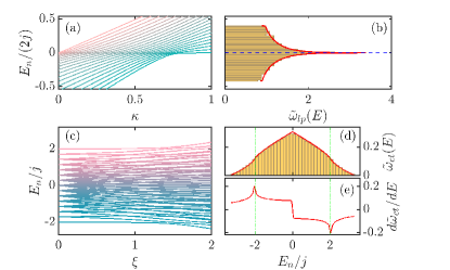
Figure 1: (a) Energy spectrum of the Lipkin model as a function of $\kappa$ with $j=N/2=20$. (b) Rescaled density of states, $\tilde{\omega}_{lp}(E)=\omega_{lp}(E)/j$, of the Lipkin model with $\kappa=0.4$ and $j=N/2=500$. The red solid line is the semiclassical result and the horizontal blue dashed line denotes the critical energy $E/(2j)=E_{c}/(2j)=0$. (c) Energy spectrum of the coupled top model as a function of $\xi$ with $j=7$. (d) Rescaled density of states, $\tilde{\omega}_{ct}(E)=\omega_{ct}(E)/j^{2}$, of the coupled top model with $\xi=3$ and $j=70$. The red solid line denotes the semiclassical result. (e) Derivative of $\tilde{\omega}_{ct}(E)$ for the coupled top model with $\xi=3$ and $j=70$. Two vertical green dot-dashed lines in panels (d) and (e) indicate the critical energies $E/j=E_{c}/j=\pm 2$ of ESQPTs in coupled top model.

For spin systems that studied in this work, the Husimi function can be calculated by using the so-called $\mathrm{SU}(2)$ spin-$j$ coherent states Zhang et al. (1990); Gazeau (2009)

$$|\zeta\rangle=(1+|\zeta|^{2})^{-j}e^{\zeta J_{+}}|j,-j\rangle,$$ (2)

where $\zeta\in\mathbb{C},J_{+}=J_{x}+iJ_{y}$ is the spin raising operator, and $|j,-j\rangle$ is the eigenstate of $J_{z}$ with eigenvalue $-j$, that is, $J_{z}|j,-j\rangle=-j|j,-j\rangle$. Here $J_{\{x,y,z\}}$ are the components of spin angular momentum operator. The coherent states is an overcomplete set and satisfy the closure relation

$$\frac{2j+1}{\pi}\int|\zeta\rangle\langle\zeta|\frac{d^{2}\zeta}{(1+|\zeta|^{2})^{2}}=\mathbf{1},$$ (3)

with $d^{2}\zeta=d\mathrm{Re}(\zeta)d\mathrm{Im}(\zeta)$ being the integration measure on $\mathbb{C}$. To visualize the Husimi function in phase space $(p,q)$, we parameterize $\zeta$ in terms of canonical variables $q$ and $p$ as de Aguiar et al. (1992); Pilatowsky-Cameo et al. (2020)

$$\zeta(p,q)=\frac{q-ip}{\sqrt{4-(p^{2}+q^{2})}},$$ (4)

with $p^{2}+q^{2}\leq 4$. Then it is straightforward to find that in phase space the closure relation Eq. (3) can be rewritten as

$$\frac{2j+1}{4\pi}\int_{\Omega}|\zeta(p,q)\rangle\langle\zeta(p,q)|dpdq=\mathbf{1},$$ (5)

where the area $\Omega$ is defined by $p^{2}+q^{2}\leq 4$. Hence the normalization condition of the Husimi function Eq. (1) in phase space is given by

$$\frac{2j+1}{4\pi}\int_{\Omega}Q(p,q)dpdq=1.$$ (6)

As is well known, a great amount of information about the features of the system can be extracted from the moments of the Husimi function Aulbach et al. (2004); Romera et al. (2012); Calixto et al. (2012); Romera et al. (2014). Among all moments, an important and useful one is the second moment (also dubbed as the generalized inverse participation ratio), which quantifies the degree of delocalization of a quantum state in phase space, and read as

$$M_{2}=\frac{2j+1}{4\pi}\int_{\Omega}Q^{2}(p,q)dpdq.$$ (7)

For an extremely extended state, the phase space is uniformly covered by state $\rho=|\psi\rangle\langle\psi|$, we would have $Q(p,q)\sim 1/(2j+1)$. In this case, one can find that $M_{2}\sim 1/(2j+1)$ which goes to zero as $j\to\infty$. Hence, the smaller is the value of $M_{2}$, the higher is the degree of delocalization of state $|\psi\rangle$ in phase space. On the other hand, if the state $\rho=|\psi\rangle\langle\psi|$ is identical to one point $(p_{0},q_{0})$ in phase space, we would expect $Q(p,q)\sim\exp{\left[-(q-q_{0})^{2}/(2\sigma_{q}^{2})+(p-p_{0})^{2}/(2\sigma_{p}^{2})\right]}$ with, according to normalization condition, $\sigma_{q}\sigma_{p}=2/(2j+1)$. In the classical limit $j\to\infty$, one can see that $Q(p,q)$ shrinks to the point $(p_{0},q_{0})$, as expected. Then, the second moment of Husimi function for this maximal localized state is given by $M_{2}\sim 1/2$. Therefore, we have $M_{2}\in[0,1/2]$ with the maximum value corresponds to the maximum localization state in phase space.

Besides the second moment of the Husimi function, another quantity that has been employed in various studies to characterize the properties of the Husimi function is the Wehrl entropy Romera et al. (2012); Calixto et al. (2012); Romera et al. (2014); Castaños et al. (2015); Calixto and Romera (2015). As the classical counterpart of the quantum von Neumann entropy, the Wehrl entropy is defined as Wehrl (1979)

$$W=-\frac{2j+1}{4\pi}\int_{\Omega}Q(p,q)\ln[Q(p,q)]dpdq.$$ (8)

Here, it is worth pointing out that the second moment $M_{2}$ in Eq. (7) can be considered as a linearized version of the Wehrl entropy. Therefore, the Wehrl entropy also measures the degree of localization of a quantum state in phase space. However, in contrast to $M_{2}$, the degree of delocalization increases with increasing $W$. For the fully extended states, we have $W_{max}\sim\ln(2j+1)$. In addition, the Lieb conjecture shows that the minimum Wehrl entropy is $W_{min}=j/(j+1)$, so that $W_{min}\to 1$ as $j\to\infty$ Lieb (2002).

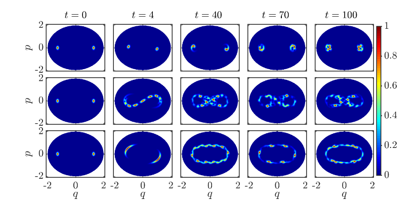
Figure 2: Snapshots of the rescaled spin Husimi function $\mathcal{Q}_{t}(p,q)=Q_{t}(p,q)/Q_{t}^{m}$ with $Q_{t}^{m}$ being the maximum value of $Q_{t}(p,q)$, at different time steps for the Lipkin model with $\eta=0.4,1,1.7$ (from top to bottom). Other parameters are: $j=N/2=200$ and $\kappa=0.4$.

More insights into the phase space features of a state can be obtained from the marginal distributions of the Husimi function for position and momentum spaces, respectively. For spin-$j$ coherent states studied in this work, they are defined as

$$Q(q)=\sqrt{\frac{2j+1}{4\pi}}\int Q(p,q)dp,$$

$$Q(p)=\sqrt{\frac{2j+1}{4\pi}}\int Q(p,q)dq,$$ (9)

with normalization conditions

$$\sqrt{\frac{2j+1}{4\pi}}\int Q(q)dq=\sqrt{\frac{2j+1}{4\pi}}\int Q(p)dp=1.$$ (10)

Accordingly, the second moment and Wehrl entropy of marginal distributions are given by

$$M_{2}^{(\mu)}=\sqrt{\frac{2j+1}{4\pi}}\int Q^{2}(\mu)d\mu,$$

$$W^{(\mu)}=-\sqrt{\frac{2j+1}{4\pi}}\int Q(\mu)\ln[Q(\mu)]d\mu,$$ (11)

where $\mu\in\{p,q\}$.

We would like to point out that the marginal distributions $Q(q),Q(p)$ of the Husimi function do not equal to the density functions $|\langle q|\psi\rangle|^{2}$ and $|\langle p|\psi\rangle|^{2}$, in sharp contrast to the case of Wigner function. In fact, they are the Gaussian smeared density distribution in position and momentum spaces, respectively Romera et al. (2012); Varga and Pipek (2003). Note further that, in general, we have $|M_{2}-M_{2}^{(p)}M_{2}^{(q)}|=\delta M_{2}\geq 0$ and $|W-[W^{(p)}+W^{(q)}]|=\delta W\geq 0$ with $\delta M_{2},\delta W$ decrease as the system size increases except around some singular points, such as quantum critical points Aulbach et al. (2004); Romera et al. (2012); Varga and Pipek (2003).

In the following, by exploiting above outlined properties of the Husimi function, we will explore the signatures of ESQPTs in two many body systems, namely the Lipkin and coupled top models.

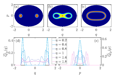
Figure 3: Rescaled long-time averaged Husimi function $\overline{\mathcal{Q}}_{lp}(p,q)=\overline{Q}_{lp}(p,q)/\overline{Q}_{lp,m}$ of the Lipkin model for (a) $\eta=0.4$, (b) $\eta=1$, and (c) $\eta=1.8$ with $j=N/2=200$ and $\kappa=0.4$. Here $\overline{Q}_{lp,m}$ denotes the maximum value of $\overline{Q}_{lp}(p,q)$. The color scale in Fig. 2 has been used for panels (a)-(c). Marginal distributions $\overline{Q}_{lp}(q)$ and $\overline{Q}_{lp}(p)$ of $\overline{Q}_{lp}(p,q)$ for several values of $\eta$ are plotted in panels (d) and (e), respectively.

III Models

III.1 Lipkin model

The Lipkin model describes $N$ spin-$1/2$ particles with infinite range of interactions and subjected to an external magnetic field. It was first introduced as a toy model to explore phase transitions in nuclear systems Lipkin et al. (1965) and since then it has been exploited as a paradigmatic model in various studies of quantum phase transitions Ribeiro et al. (2008); Engelhardt et al. (2013); Botet and Jullien (1983); Dusuel and Vidal (2005); Castaños et al. (2006); Campbell (2016). As the Lipkin model has broad applications in several different fields of physics, it has attracted much attention from both theoretical Bao et al. (2020); Lourenço et al. (2020); Russomanno et al. (2017); Huang et al. (2018) and experimental Morrison and Parkins (2008); Zibold et al. (2010) perspectives in recent years.

By using the collective operators $J_{\alpha}=\sum_{k}^{N}\sigma_{k}^{\alpha}/2,\{\alpha=x,y,z\}$ with $\sigma_{k}^{\alpha}$ is the $\alpha$th component of the Pauli matrix of $k$th spin, the Hamiltonian of the Lipkin model can be written as

$$H_{lp}=-\frac{4(1-\kappa)}{N}J^{2}_{x}+\kappa\left(J_{z}+\frac{N}{2}\right),$$ (12)

where $\kappa$ denotes the strength of the external magnetic field. The total spin operator $\mathbf{J}^{2}=\mathbf{J}_{x}^{2}+\mathbf{J}_{y}^{2}+\mathbf{J}_{z}^{2}$ with eigenvalue $j(j+1)$ is commutated with the Hamiltonian. In our study, we restrict ourself in the spin sector with $j=N/2$, thus the dimension of the Hamiltonian matrix is $\mathcal{D}_{H_{lp}}=N+1$. Moreover, due to conservation of the parity operator $\hat{\Pi}_{lp}=e^{i\pi(j-m)}$ with $m\in\{-j,-j+1,\ldots,j\}$ is the eigenvalue of $J_{z}$, the Hamiltonian matrix is further split into even- and odd- parity blocks with dimensions $\mathcal{D}_{H_{lp}}^{e}=N/2+1$ and $\mathcal{D}_{H_{lp}}^{o}=N/2$, respectively. We focus on the even-parity block which includes the ground state of the system.

The Lipkin model undergoes a second-order ground state quantum phase transition from the paramagnetic phase with $\kappa<4/5$ to the ferromagnetic phase with $\kappa>4/5$ at the critical point $\kappa_{c}=4/5$ Botet and Jullien (1983); Dusuel and Vidal (2005); Castaños et al. (2006). The ground state quantum phase transition of the Lipkin model has been studied extensively in numerous works Botet and Jullien (1983); Dusuel and Vidal (2005); Castaños et al. (2006); Campbell (2016); Bao et al. (2020); Lourenço et al. (2020); Latorre et al. (2005); Titum and Maghrebi (2020). In particular, the phase space characters of the ground state quantum phase transition of the Lipkin model has been explored in Ref. Romera et al. (2014). Here, we are interested in analyzing the signatures of ESQPT in phase space by means of the Husimi function. The Lipkin model exhibits an ESQPT at critical energy $E_{c}=0$ when $\kappa<4/5$ Caprio et al. (2008); Pérez-Fernández et al. (2009). The ESQPT in Lipkin model is characterized by the singular behavior in its density of states $\omega_{lp}(E)=\sum_{n}\delta(E-E_{n})$.

In Fig. 1(a), we plot the energy levels of the Lipkin model with $j=N/2=20$ as a function of $\kappa$. We can see that the energy levels exhibit an obvious collapse around $E_{c}=0$ for the cases of $\kappa<4/5$. This means the density of states of the Lipkin model would have a sharp peak in the neighborhood of $E_{c}$. Indeed, as can be seen from Fig. 1(b), both the numerical and semiclassical results Pérez-Fernández et al. (2009) show that, at the critical energy $E_{c}=0$, $\omega_{lp}(E)$ has a cusp singular which turns into a logarithmic divergence as $j=N/2\to\infty$ Ribeiro et al. (2008); Stránský et al. (2014).

III.2 Coupled top model

The second model we considered is the so-called coupled top model, also known as the Feingold-Peres model Feingold and Peres (1983); Feingold et al. (1984); Hines et al. (2005); Fan et al. (2017); Mondal et al. (2020). It describes the interaction between two larger spins with respective angular momentum operators $\mathbf{J}_{1}=(J_{1x},J_{1y},J_{1z})$ and $\mathbf{J}_{2}=(J_{2x},J_{2y},J_{2z})$, whose Hamiltonian takes the form

$$H_{ct}=J_{1z}+J_{2z}+\frac{\xi}{j}J_{1x}J_{2x},$$ (13)

where $\xi$ is the coupling strength between two spins. Here, we assume two spins have same magnitude $\mathbf{J}_{1}^{2}=\mathbf{J}_{2}^{2}=j(j+1)$, so that the dimension of the Hilbert space is $\mathcal{D}_{H_{ct}}=(2j+1)^{2}$. However, as the Hamiltonian in Eq. (13) remains invariant under the permutation symmetry $\hat{\mathscr{P}}$ between two spins $(J_{1}\leftrightarrow J_{2})$ and under parity $\hat{\Pi}_{ct}=e^{i\pi(2j-m_{1}-m_{2})}$ with $m_{1},m_{2}\in\{-j,-j+1,\ldots,j\}$ are the eigenvalues of $J_{1z},J_{2z}$, the Hilbert space can be further decomposed into four subspaces according to the eigenvalues of $\hat{\mathscr{P}}$ and $\hat{\Pi}_{ct}$. We shall focus on the subspace identified by $\mathscr{P}=+1,\Pi_{ct}=+1$, denoted by $V_{++}$, which contains the ground state. We also restrict to integer $j$, thus the dimension of $V_{++}$ is $\mathcal{D}_{V_{++}}=(j+1)^{2}$ Fan et al. (2017).

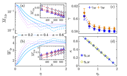
Figure 4: (a) Second moment of $\overline{Q}_{lp}(p,q)$ as a function of $\eta$ for several $\kappa$ with $j=N/2=200$ (solid lines) and $j=N/2=400$ (dashed lines). Inset: Critical second moment, $\overline{M}_{2,lp}^{c}=\overline{M}_{2,lp}(\eta_{c})$, as a function of $N$ for $\eta_{c}=1.5$ (triangles), $\eta_{c}=1$ (squares), and $\eta_{c}=0.5$ (diamonds). Red dashed lines are of the form $\overline{M}_{2,lp}^{c}\sim N^{-\gamma_{M}}$. (b) Wehrl entropy of $\overline{Q}_{lp}(p,q)$ as a function of $\eta$ for various $\kappa$ with $j=N/2=200$ (solid lines) and $j=N/2=400$ (dashed lines). Inset: Critical Wehrl entropy, $\overline{W}_{lp}^{c}=\overline{W}_{lp}(\eta_{c})$, as a function of $N$ for $\eta_{c}=1.5$ (triangles), $\eta_{c}=1$ (squares), and $\eta_{c}=0.5$ (diamonds). Red dotted lines are of the form $\overline{W}_{lp}^{c}\sim\gamma_{W}\ln(N)$. (c) Values of the finite size scaling exponents of $\overline{M}_{2,lp}^{c}$ and $\overline{W}_{lp}^{c}$ for several $\eta_{c}$ with $j=N/2=200$. (d) Critical values $\eta_{c,M},\eta_{c,W}$ estimated from the extrema of $\overline{M}_{2,lp}$ and $\overline{W}_{lp}$, respectively, for different values of $\kappa$ with $j=N/2=400$. The dot-dashed line indicates the analytical result in Eq. (14).

The coupled top model has been studied extensively in diverse fields of physics Hines et al. (2005); Fan et al. (2017); Mondal et al. (2020); Robb and Reichl (1998); Ray et al. (2019). It is known that its ground state displays a second-order quantum phase transition at $\xi_{c}=1$, which separates the ferromagnetic phase with $\xi<\xi_{c}$ from the paramagnetic phase with $\xi>\xi_{c}$ Hines et al. (2005); Mondal et al. (2020). In particular, it has been found that the coupled top model undergoes ESQPTs at critical energies $E_{c}/j=\pm 2$ for $\xi>\xi_{c}=1$. Different from the case of Lipkin model, the ESQPTs in the coupled top model are identified by the non-analytical behaviors in the derivative of the density of states at the critical energies. A very similar signature of ESQPT has also been founded in the Dicke model Brandes (2013); Bastarrachea-Magnani et al. (2014).

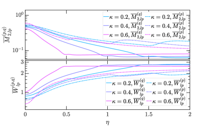
Figure 5: Second moment (upper panel) and Wehrl entropy (bottom panel) of the marginal distributions of $\overline{Q}_{lp}(p,q)$ as a function of $\eta$ for several $\kappa$ with $j=N/2=200$.

The energy spectrum of the coupled top model as a function of control parameter $\xi$ is plotted in panel (c) of Fig. 1 for $j=7$. We see that the energy spectrum becomes more complex as the value of $\xi$ increases. However, the collapse of the energy levels around the critical energy observed in the Lipkin model [cf. Fig. 1(a)] does not exist in the energy spectrum of the coupled top model. This means the density of states of the coupled top model, denoted by $\omega_{ct}(E)$, will behave as a continuous function of energy at $\xi>\xi_{c}$, as is shown in Fig. 1(d) for the numerical and associated semiclassical results Mondal et al. (2020). In fact, the ESQPTs in the coupled top model are uncovered through the singular behaviors in the derivative of $\omega_{ct}(E)$. In panel (e) of Fig. 1, we plot the derivative of $\tilde{\omega}_{ct}(E)=\omega_{ct}(E)/j^{2}$ as a function of $E_{n}/j$ with $j=70$. As it can be seen, $d\tilde{\omega}_{cp}(E)/dE$ develops a cusp singular at the critical energies. Such singularities are expect to be the logarithmic divergences in the thermodynamic limit $j\to\infty$ Stránský et al. (2014); Stránský and Cejnar (2016). In the following, we will constraint ourselves to the critical energy $E_{c}/j=-2$, since $E_{c}/j=2$ gives rise the same results.

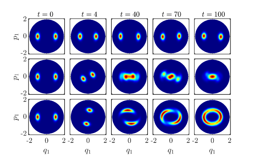
Figure 6: Snapshots of the rescaled spin Husimi function $\mathcal{Q}_{t}(p_{1},q_{1})=Q_{t}(p_{1},q_{1})/Q_{t}^{m}(p_{1},q_{1})$ with $Q_{t}^{m}(p_{1},q_{1})$ being the maximum value of $Q_{t}(p_{1},q_{1})$, at different time steps for the coupled top model with $\xi_{1}=2.5,1.5,0.5$ (from top to bottom). Other parameters are: $j=30$ and $\xi_{0}=3$. The color scale of figure 2 has been used.

IV Results and discussions

In this section, we discuss how to identify the signatures of ESQPT from the perspective of quantum phase space by means of the Husimi function in two aforementioned models. We consider the the impacts of ESQPT on the dynamical features of Husimi function using the quantum quench protocol and focus on the properties of the long-time averaged Husimi function.

IV.1 Husimi function of the Lipkin model

For the Lipkin model, the quantum quench protocol is described as follows. The model is initially prepared in the ground state $|\psi_{0}\rangle$ of $H_{lp}$ with $0<\kappa<4/5$. At $t=0^{+}$, we suddenly add an external magnetic field along $z$ direction with strength $\eta$, and let the model evolve under the Hamiltonian $H_{lp}^{f}=H_{lp}+\eta(S_{z}+N/2)$. For a certain value of $\kappa$, one can take the model crossing of the critical energy of ESQPT by varying the strength of $\eta$. The critical strength $\eta_{c}$, which leads to the critical energy $E_{c}=0$, can be obtained through the coherent state approach and is given by Relaño et al. (2008); Pérez-Fernández et al. (2009)

$$\eta_{c}=2-\frac{5}{2}\kappa,$$ (14)

with $0<\kappa<4/5$. We stress that the critical strength $\eta_{c}$ for the ESQPT is smaller than the quench strength which drive the model through the ground state quantum phase transition Pérez-Fernández et al. (2009).

The quantum state of the model is evolved as $\rho(t)=|\psi(t)\rangle\langle\psi(t)|=e^{-iH_{lp}^{f}t}\rho(0)e^{iH_{lp}^{f}t}$ with $\rho(0)=|\psi_{0}\rangle\langle\psi_{0}|$. Hence the Husimi function at time $t$ can be written as

$$Q_{t}(p,q) =\langle\zeta(p,q)|\rho(t)|\zeta(p,q)\rangle$$

$$=\left|\sum_{n}e^{-iE_{n}t}\langle\zeta(p,q)|E_{n}\rangle\langle E_{n}|\psi_{0}\rangle\right|^{2},$$ (15)

where $|E_{n}\rangle$ is the $n$th eigenstate of $H_{lp}^{f}$ with eigenvalue $E_{n}$. Here we see that $Q_{t}(p,q)$ is strongly depended on the transition amplitudes between the initial state and the $n$th eigenstate of $H_{lp}^{f}$.

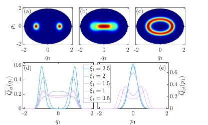
Figure 7: Rescaled long-time averaged Husimi function $\overline{\mathcal{Q}}_{ct}(p_{1},q_{1})=\overline{Q}_{ct}(p_{1},q_{1})/\overline{Q}_{ct,m}$ of the coupled top model for (a) $\xi_{1}=2.5$, (b) $\xi_{1}=1.5$, and (c) $\xi_{1}=0.5$ with $j=30$ and $\xi_{0}=3$. Here $\overline{Q}_{ct,m}$ denotes the maximum value of $\overline{Q}_{ct}(p_{1},q_{1})$. The color scale in Fig. 2 has been employed for panels (a)-(c). Marginal distributions $\overline{Q}_{ct}(q_{1})$ and $\overline{Q}_{ct}(p_{1})$ of $\overline{Q}_{ct}(p_{1},q_{1})$ for several values of $\xi_{1}$ are plotted in panels (d) and (e), respectively.

In Fig. 2, we plot the Husimi function of the Lipkin model at different time steps for several values of $\eta$ with $\kappa=0.4$ and $N=400$. For this case, the critical quench strength in Eq. (14) is $\eta_{c}=1$. We first note that the ground state in the even-parity sector can be well described by the so-called even coherent states Castaños et al. (2006); Romera et al. (2014); Dodonov et al. (1974), $|\zeta(p,q)\rangle_{+}=\mathcal{N}_{+}(p,q)[|\zeta(p,q)\rangle+|\zeta(-p,-q)\rangle]$, with $\mathcal{N}_{+}(p,q)=1/\sqrt{2\{1+[1-(p^{2}+q^{2})/2]^{2j}\}}$ is the normalization constant. As a result, the Husimi function of initial state should be represented by two symmetrically localized packets in phase space, as seen in the first column of Fig. 2. As time increases, the Husimi function exhibits remarkable different behaviors for $\eta$ below, at, and above the critical value $\eta_{c}=1$. Specifically, as observed in the top row of Fig. 2, the Husimi function remains as two distinct localized packets in its time evolution for $\eta<\eta_{c}$. At the critical point $\eta=\eta_{c}$ [see the second row in Fig. 2], the evolution of the Husimi function results in an extension in phase space and, in particular, two initially disconnected packets are joined together in this case. Finally, when $\eta>\eta_{c}$, the two initially separated packets are merged into a single one and the evolution of the Husimi function is in sharp contrast to the case of $\eta<\eta_{c}$, as illustrated in the last row of Fig. 2. The strikingly distinct behaviors in the dynamics of Husimi function on two sides of the transition suggest that the underlying ESQPT has non-trivial impacts on the dynamics of the model. Moreover, the particular dynamical behavior of Husimi function at $\eta=\eta_{c}$ can be employed to probe the occurrence of an ESQPT.

To get more evident signatures of ESQPT, we consider the long-time averaged Husimi function

$$\overline{Q}(p,q)=\langle\zeta(p,q)|\bar{\rho}|\zeta(p,q)\rangle,$$ (16)

where $\bar{\rho}$ is the long-time averaged state of the model and defined as

$$\bar{\rho}=\lim_{T\to\infty}\frac{1}{T}\int_{0}^{T}\rho(t)dt.$$ (17)

For the Lipkin model, it is straightforward to find that the explicit expression of the long-time averaged Husimi function is given by

$$\overline{Q}_{lp}(p,q)=\sum_{n}|\langle\zeta(p,q)|E_{n}\rangle|^{2}|\langle E_{n}|\psi_{0}\rangle|^{2}.$$ (18)

Here we see again the transition probabilities between $|\psi_{0}\rangle$ and the $n$th eigensate of $H_{lp}^{f}$ play crucial role in determining the behaviors of $\overline{Q}_{lp}(p,q)$.

In Figs. 3(a)-3(c), we plot $\overline{Q}_{lp}(p,q)$ for various values of $\eta$. We see that the structure of $\overline{Q}_{lp}(p,q)$ changes drastically as $\eta$ passes through the critical point. For $\eta<\eta_{c}$, $\overline{Q}_{lp}(p,q)$ consists of two localized and disconnected parts. With increasing $\eta$, the extension of $\overline{Q}_{lp}(p,q)$ leads to two disconnected parts joining together at $\eta=\eta_{c}=1$. As $\eta$ increases further, the two joined parts are merged into a single one. We also note that $\overline{Q}_{lp}(p,q)$ has a rather larger degree of delocalization at $\eta=\eta_{c}$. The features of $\overline{Q}_{lp}(p,q)$ are more visible in its marginal distributions [cf. Eq.(II)]. For several values of $\eta$, the marginal distributions $\overline{Q}_{lp}(q)$ and $\overline{Q}_{lp}(p)$ are plotted in Figs. 3(d) and 3(e), respectively. Clearly, the width of $\overline{Q}_{lp}(q)$ and $\overline{Q}_{lp}(p)$ increase with increasing $\eta$ due to the extension of $\overline{Q}_{lp}(p,q)$ in phase space. Moreover, an obvious complex shape in the marginal distributions at $\eta_{c}=1$ implies that they act as indicators of the ESQPT, in particular for the case of $\overline{Q}_{lp}(q)$.

To further elucidate the signatures of ESQPT in the properties of $\overline{Q}_{lp}(p,q)$, we evaluate its second moment $\overline{M}_{2,lp}$ [see Eq. (7)] and Wehrl entropy $\overline{W}_{lp}$ [see Eqs. (8)]. In Figs. 4(a) and 4(b), we plot $\overline{M}_{2,lp}$ and $\overline{W}_{lp}$ as a function of $\eta$ for several values of $\kappa$. We see that both the second moment and Wehrl entropy reach their extremum value at the critical value $\eta_{c}$. This means that the underlying ESQPT gives rise to a maximal extension of the quantum state. Moreover, the extremum values in the second moment and Wehrl entropy, denoted by $\overline{M}_{2,lp}^{c}$ and $\overline{W}^{c}_{lp}$, increase with increasing the system size $N$. In the insets of Fig. 4(a) and 4(b), we show how $\overline{M}^{c}_{2,lp}$ and $\overline{W}^{c}_{lp}$ vary with $N$ for several values of $\eta_{c}$. We find that $\overline{M}_{2,lp}^{c}$ follows a power law scaling $\overline{M}_{2,lp}^{c}\sim N^{-\gamma_{M}}$, regardless of the value of $\eta_{c}$. However, in all cases, $\overline{W}_{lp}^{c}$ exhibits a logarithmic scaling of the form $\overline{W}_{lp}^{c}\sim\gamma_{W}\ln(N)$. The values of the scaling exponents $\gamma_{M}$ and $\gamma_{W}$ are demonstrated in Fig. 4(c). As it can be seen, $\gamma_{M}$ and $\gamma_{W}$ decrease with an increases in $\eta_{c}$. By identifying the position of the extremum in $\overline{M}_{2,lp}$ and $\overline{W}_{lp}$ as the estimation of the critical point, we compare the numerically obtained critical points with the analytical ones in Eq. (14). A good agreement between them can be clearly observed in Fig. 4(d). These results suggest that the second moment and Wehrl entropy of $\overline{Q}_{lp}(p,q)$ can reliably detect ESQPTs in Lipkin model.

Figure 5 displays the variation of the second moment and Wehrl entropy of the marginal distributions with $\eta$ for several values $\kappa$. The underlying ESQPT induces the remarkable changes in the behaviors of the marginal quantities, as is evident from Fig. 5. We further note that the extension of the quantum state in position direction is larger than that in momentum direction consistent with the behaviors of the marginal distributions observed in Figs. 3(d) and 3(e).

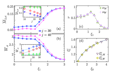
Figure 8: (a) Second moment of $\overline{Q}_{ct}(p_{1},q_{1})$ as a function of $\xi_{1}$ for different system size $j$ with $\xi_{0}=3$ and $\xi_{1}^{c}=1.5$ [see Eq. (19)]. Inset: $\overline{M}_{2,ct}$ as a function of $j$ at $\xi_{1}=0.3$ (blue squares), $\xi_{1}=1.5$ (red circles), and $\xi_{1}=2.7$ (green diamonds). The dashed lines are of the form $\overline{M}_{2,ct}\sim j^{-\nu_{M}}$. (b) Wehrl entropy of $\overline{Q}_{ct}(p_{1},q_{1})$ as a function of $\xi_{1}$ for different $j$ with $\xi_{0}=3$. Inset: $\overline{W}_{ct}$ as a function of $j$ for $\xi_{1}=0.3$ (blue squares), $\xi_{1}=1.5$ (red circles), and $\xi_{1}=2.7$ (green diamonds). The dotted lines are of the form $\overline{W}_{ct}\sim\nu_{W}\ln(j)$. (c) Finite size scaling exponents $\nu_{M}$ and $\nu_{W}$ as a function of $\xi_{1}$ with $\xi_{0}=3$. (d) Estimated critical points $\xi_{1,M}^{c},\xi_{1,W}^{c}$, obtained from the minima in $d\nu_{M(W)}/d\xi_{1}$, as a function of $\xi_{0}$. The dot-dashed line denotes the analytical result in Eq. (19).

IV.2 Husimi function of the coupled top model

To analyze the ESQPT in the coupled top model, the quench protocol consists as follows. Initially, the ground state $|\Psi_{0}\rangle$ of $H_{ct}$ with $\xi=\xi_{0}>1$ is prepared. Then we suddenly change the coupling strength from $\xi_{0}$ to $\xi_{1}$ and consider the evolution of the model governed by the Hamiltonian $H_{ct}(\xi_{1})$. The critical coupling strength, denoted by $\xi_{1}^{c}$, is identified as the coupling that takes the energy of $H_{ct}(\xi_{1})$ to the critical energy of the ESQPT, so that $\langle\psi(\xi_{0})|H_{ct}(\xi_{1}^{c})|\psi(\xi_{0})\rangle/j=E_{c}/j=-2$. By using the semiclassical approach (see Appendix A), one can find $\xi_{1}^{c}$ is given by

$$\xi_{1}^{c}=\frac{2\xi_{0}}{\xi_{0}+1},$$ (19)

with $\xi_{0}>1$. The critical coupling of the ESQPT depends on the value of $\xi_{0}$ and is always larger than the ground state critical point $\xi_{c}=1$.

The evolved state of the model is $\rho_{t}(\xi_{1})=|\Psi_{t}\rangle\langle\Psi_{t}|=e^{-iH(\xi_{1})t}\rho_{0}(\xi_{0})e^{iH(\xi_{1})t}$ with $\rho_{0}(\xi_{0})=|\Psi_{0}\rangle\langle\Psi_{0}|$. As the phase space of the coupled top model has $4$ dimensions, the evolved Husimi function expressed in terms of $\rho_{t}(\xi_{1})$ takes the form

$$Q_{t}({\bf p},{\bf q})=\langle\Upsilon({\bf p},{\bf q})|\rho_{t}(\xi_{1})|\Upsilon({\bf p},{\bf q})\rangle,$$ (20)

where ${\bf p}=(p_{1},p_{2})$, ${\bf q}=(q_{1},q_{2})$, and $|\Upsilon({\bf p},{\bf q})\rangle=|\zeta(p_{1},q_{1})\rangle\otimes|\zeta(p_{2},q_{2})\rangle$ with

$$\zeta(p_{k},q_{k})=\frac{q_{k}-ip_{k}}{\sqrt{4-(p_{k}^{2}+q_{k}^{2})}},\qquad k=1,2.$$

The normalization condition for $Q_{t}({\bf p},{\bf q})$ reads

$$\left(\frac{2j+1}{4\pi}\right)^{2}\int_{\Omega_{1}}\int_{\Omega_{2}}Q_{t}({\bf p},{\bf q})d{\bf p}d{\bf q}=1,$$ (21)

where $\Omega_{1}\in\{(p_{1},q_{1})|p_{1}^{2}+q_{1}^{2}\leq 4\}$ and $\Omega_{2}\in\{(p_{2},q_{2})|p_{2}^{2}+q_{2}^{2}\leq 4\}$.

The four-dimensional Husimi function $Q_{t}({\bf p},{\bf q})$ is difficult to display. Therefore, we consider the projection of the Husimi function over the space $(p_{1},q_{1})$, so that $Q_{t}(p_{1},q_{1})\sim\int dp_{2}dq_{2}Q_{t}({\bf p},{\bf q})$. As the coherent states $|\zeta(p_{2},q_{2})\rangle$ in the space $(p_{2},q_{2})$ fulfill the normalization condition [cf. Eq. (3)], the projected Husimi function adopts the form

$$Q_{t}(p_{1},q_{1})=\langle\zeta(p_{1},q_{1})|\rho_{1}^{t}(\xi_{1})|\zeta(p_{1},q_{1})\rangle,$$ (22)

with normalization condition

$$\frac{2j+1}{4\pi}\int_{\Omega_{1}}Q_{t}(p_{1},q_{1})dp_{1}dq_{1}=1.$$

Here $\rho_{1}^{t}(\xi_{1})=\mathrm{Tr}_{2}[\rho_{t}(\xi_{1})]$ is the reduced density matrix of the first spin.

In Fig. 6, we show the snapshots of the evolution of Husimi function at several time steps for different values of $\xi_{1}$ with $\xi_{0}=3$. The critical value of $\xi_{1}$ for $\xi_{0}=3$ is $\xi_{1}^{c}=1.5$ [cf. Eq. (19)]. The ground state of the coupled top model has even-parity and it can be well approximated by the even coherent states. The Husimi function at the initial time should consist of two distinct wave packets, which are symmetrically placed in the phase space, as seen in the first column of Fig. 6. As time increases, the Husimi function of the coupled top model exhibits a very similar behaviors as observed in the Lipkin model [cf. Fig. 2]. Namely, the evolution of the Husimi function remains as two different wave packets until $\xi_{1}=\xi_{1}^{c}$, where two separated wave packets are joined together. Further decreases $\xi_{1}$ gives rise to two disconnected wave packets are emerged into a single one at large time. Therefore, as in the Lipkin model, the ESQPT in the coupled top model can also be identified through the particular dynamics of the Husimi function.

More evident signatures of ESQPT are revealed in the features of long-time averaged Husimi function Eq. (16). For the coupled top model, it can be written as

$$\overline{Q}_{ct}(p_{1},q_{1})=\langle\zeta(p_{1},q_{1})|\overline{\rho}_{1}(\xi_{1})|\zeta(p_{1},q_{1})\rangle,$$ (23)

where $\overline{\rho}_{1}(\xi_{1})=\mathrm{Tr}_{2}[\overline{\rho}(\xi_{1})]$ with

$$\overline{\rho}(\xi_{1})=\lim_{T\to\infty}\frac{1}{T}\int_{0}^{T}\rho_{t}(\xi_{1})dt.$$

In the eigenstates of the post-quench Hamiltonian $H_{ct}(\xi_{1})$, denoted by $\{|E_{n}\rangle\}$, it is then straight to find that $\overline{Q}_{ct}(p_{1},q_{1})$ can be calculated as

$$\overline{Q}_{ct} (p_{1},q_{1})$$

$$=\sum_{n}|\langle\Psi_{0}|E_{n}\rangle|^{2}\langle\zeta(p_{1},q_{1})|\rho_{1}^{(n)}(\xi_{1})|\zeta(p_{1},q_{1})\rangle,$$ (24)

where $\rho_{1}^{(n)}(\xi_{1})=\mathrm{Tr}_{2}(|E_{n}\rangle\langle E_{n}|)$. As we found in the Lipkin model, $\overline{Q}_{ct}(p_{1},q_{1})$ of the coupled top model also depends on the transition probabilitites between the initial state and the $n$th eigenstate of $H_{ct}(\xi_{1})$.

In Figs. 7(a)-7(c), we plot $\overline{Q}_{ct}(p_{1},q_{1})$ for different values of $\xi_{1}$ with $\xi_{0}=3$ and $j=30$. With decreasing $\xi_{1}$, the Husimi function exhibits a remarkable change as soon as $\xi_{1}\leq\xi_{1}^{c}=1.5$. The ESQPT at $\xi_{1}^{c}=1.5$ is clearly associated with a significant extension of the Husimi function in phase space. The dramatical changes of $\overline{Q}_{ct}(p_{1},q_{1})$ in phase space with decreasing $\xi_{1}$ are more visible in its marginal distributions, as depicted in panels (d) and (e) of Fig. 7. Consequently, the ESQPT in the coupled top model is signified as the dramatical extension of the Husimi function in phase space, as observed in the Lipkin model.

To provide further insights into the phase space signatures of ESQPT in the coupled top model, we consider the second moment and Wehrl entropy of $\overline{Q}_{ct}(p_{1},q_{1})$. In Figs. 8(a) and 8(b), we plot, respectively, $\overline{M}_{2,ct}$ and $\overline{W}_{ct}$ as a function of $\xi_{1}$ with $\xi_{0}=3$. The critical value of $\xi_{1}$ for $\xi_{0}=3$ is $\xi_{1}^{c}=1.5$. The dramatic change in the behaviors of $\overline{M}_{2,ct}$ and $\overline{W}_{ct}$ as $\xi_{1}$ passes through its critical value are clearly visible. For $\xi_{1}<\xi_{1}^{c}=1.5$, $\overline{M}_{2,ct}$ ($\overline{W}_{ct}$) is fixed at some smallest (largest) value, which decreases (increases) with increasing $j$, indicating that the Husimi function has maximum extension in this phase. Contrasting with $\xi_{1}<\xi_{1}^{c}$, we observe $\overline{M}_{2,ct}$ ($\overline{W}_{ct}$) increases (decreases) as $\xi_{1}$ increases when $\xi>\xi_{1}^{c}$. These results suggest that the largest extension of the Husimi function in phase space can be considered as one of signatures of ESQPT. We further find that $\overline{M}_{2,ct}$ follows a power law scaling of the form $\overline{M}_{2,ct}\sim j^{\nu_{M}}$ with scaling exponent $\nu_{M}$ depends on the value of $\xi_{1}$, as seen in the inset of Fig. 8(a). On the other hand, the Wherl entropy exhibits a logarithmic scaling $\overline{W}_{ct}\sim\nu_{W}\ln(j)$ with $\nu_{W}$ varies with $\xi_{1}$ [inset in Fig. 8(b)]. The dependences of $\nu_{M}$ and $\nu_{W}$ on $\xi_{1}$ are shown in Fig. 8(c). We see that, as a function of $\xi_{1}$, both $\nu_{M}$ and $\nu_{W}$ behave differently in the two phase. In particular, a rapid decrease in $\nu_{M}$ and $\nu_{W}$ is clearly visible around the critical point. This leads us to identify the critical point of ESQPT as the location of the minima points in the derivatives of $\nu_{M}$ and $\nu_{W}$ with respect to $\xi_{1}$. Our numerically estimated critical points, together with the analytical ones obtained from Eq. (19) are plotted in Fig. 8(d). A good agreement between the numerical and analytical results can be clearly seen.

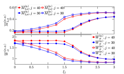
Figure 9: Second moment (upper panel) and Wehrl entropy (bottom panel) of the marginal distributions of $\overline{Q}_{ct}(p_{1},q_{1})$ as a function of $\xi_{1}$ for different $j$ with $\xi_{0}=3$.

In Fig. 9, we show the second moment and Wehrl entropy of the marginal distributions of the Husimi function as a function of $\xi_{1}$ for different system size with $\xi_{0}=3$. As expected, the behaviors of the marginal quantities change dramatically as the system crossing of the critical point of ESQPT. Moreover, as observed in Lipkin model, the Husimi function of the coupled top model also exhibits a larger degree of extension in the position direction.

V Conclusions

We have studied the phase space signatures of ESQPTs by means of Husimi function in two different models, namely Lipkin and coupled top model, both of them exhibit a second-order ESQPT at certain critical energy. We showed that the phase space signatures of ESQPT can be identified through different properties of Husimi function and its marginal distributions. We found that the different phases of ESQPT are revealed by distinct dynamical behaviors of the Husimi function and the particular dynamics of the Husimi function is able to detect the presence of ESQPT in both models. We also demonstrate that the long time average of the Husimi function exhibits strikingly distinct features in different phases of ESQPT. The transition of the long time averaged Husimi function from two symmetrically localized wave packets to a single extended wave packet can be recognized as the main signature of ESQPTs in phase space. To quantity the phase space spreading of the long time averaged Husimi function, we further investigated the properties of the second moment and Wherl entropy of the long time averaged Husimi function and its marginal distributions. The singular features observed in their second moment and Wherl entropy represent a visible manifestation of ESQPT. In turn, we employed these singular features to estimate the critical point of ESQPT and seen a good agreement between the numerical estimations and the analytical results.

Our findings confirm that phase space methods represents a powerful tool to understand ESQPTs of many body systems, extending the previous works that focus on the phase space signatures of the ground state quantum phase transitions. As ESQPTs studied in this work are quite general, we anticipate that the ESQPTs in other systems, such as Rabi Puebla et al. (2016) and Dicke models Brandes (2013); Bastarrachea-Magnani et al. (2014), will exhibit same signatures in phase space. It is an interesting future prospect to systematically explore the phase space signatures of ESQPTs in various many body systems. Another interesting extension of the present work would be to explore the phase space signatures of the first-order ESQPTs, which characterized by the discontinuity of the density of states Stránský and Cejnar (2016). Finally given the Husimi function has been measured in several experiments Eichler et al. (2011); Bohnet et al. (2016); Bouchard et al. (2017), and the realizations of the models studied in this work in quantum simulators Tian et al. (2020); Zibold et al. (2010); Strobel et al. (2014); Hines et al. (2005), we expect that our results can be experimentally tested.

Appendix A Critical point of ESQPT in the coupled top model

In the semiclassical approach, the energy surface of the system is the expectation value of the Hamiltonian in the coherent state. Therefore, the rescaled energy surface of the coupled top model is given by

$$\mathcal{E}(p_{1},q_{1},p_{2},q_{2})=\langle\Upsilon({\bf p},{\bf q})|H_{ct}|\Upsilon({\bf p},{\bf q})\rangle/j,$$ (25)

where $|\Upsilon({\bf p},{\bf q})\rangle=|\zeta(p_{1},q_{1})\rangle\otimes|\zeta(p_{2},q_{2})\rangle$ with ${\bf p}=(p_{1},p_{2})$ and ${\bf q}=(q_{1},q_{2})$. By using the relations

$$\langle\zeta|J_{+}|\zeta\rangle=\frac{2j\zeta^{\ast}}{1+|\zeta|^{2}},\quad\langle\zeta|J_{-}|\zeta\rangle=\frac{2j\zeta}{1+|\zeta|^{2}},$$

$$\langle\zeta|J_{z}|\zeta\rangle=j\left(\frac{|\zeta|^{2}-1}{|\zeta|^{2}+1}\right),$$ (26)

with $J_{\pm}=J_{x}\pm iJ_{y}$, it is straightforward to find that the rescaled energy surface of the coupled top model can be written as

$$\mathcal{E}({\bf p}, {\bf q})=\frac{1}{2}(p_{1}^{2}+q_{1}^{2})+\frac{1}{2}(p_{2}^{2}+q_{2}^{2})-2$$

$$+\frac{\xi}{4}q_{1}q_{2}\sqrt{4-(p_{1}^{2}+q_{1}^{2})}\sqrt{4-(p_{2}^{2}+q_{2}^{2})}.$$ (27)

The fixed points correspond to the values $({\bf p}_{f},{\bf q}_{f})$ that produce the ground state energy of $H_{ct}$ are obtained by minimizing $\mathcal{E}({\bf p},{\bf q})$ with respect to ${\bf p}$ and ${\bf q}$ for a given value of $\xi_{0}$. The final results are given by

$$( {\bf p}_{f},{\bf q}_{f})=(p^{f}_{1},p^{f}_{2},q^{f}_{1},q^{f}_{2})$$

$$=\begin{cases}(0,0,0,0)\quad&\text{for }\xi\leq 1,\\ (0,0,\pm\sqrt{\frac{2(\xi-1)}{\xi}},\mp\sqrt{\frac{2(\xi-1)}{\xi}})\quad&\text{for }\xi>1,\end{cases}$$ (28)

with energies

$$\mathcal{E}_{m}=\begin{cases}-2\quad&\text{for }\xi\leq 1,\\ -\left(\xi+\frac{1}{\xi}\right)\quad&\text{for }\xi>1.\end{cases}$$ (29)

For the ground state $|\Psi_{0}\rangle$ of pre-quench $H_{ct}$ with $\xi=\xi_{0}>1$, the energy of the post-quench Hamiltonian $H_{ct}(\xi_{1})$ is given by

$$\mathcal{E}(\xi_{0},\xi_{1})=\langle\Psi_{0}|H_{ct}(\xi_{1})|\Psi_{0}\rangle.$$ (30)

As $|\Psi_{0}\rangle=|\Upsilon({\bf p}_{f},{\bf q}_{f})\rangle$, the explicit expression of $\mathcal{E}(\xi_{0},\xi_{1})$ can be written as

$$\mathcal{E}(\xi_{0},\xi_{1})=\frac{(\xi_{0}-1)[2\xi_{0}-\xi_{1}(\xi_{0}+1)]}{\xi_{0}^{2}}-2.$$ (31)

For the critical quench $\xi_{1}^{c}$, we have $\mathcal{E}(\xi_{0},\xi_{1}^{c})=-2$. Hence, the critical quench $\xi_{1}^{c}$ is given by

$$\xi_{1}^{c}=\frac{2\xi_{0}}{\xi_{0}+1},$$ (32)

with $\xi_{0}>1$.

References

- Weyl (1927) H. Weyl, Z. Phys. 46, 1 (1927).
- Wigner (1932) E. Wigner, Phys. Rev. 40, 749 (1932).
- Weyl (1950) H. Weyl, The theory of groups and quantum mechanics (Courier Corporation, 1950).
- Zachos et al. (2005) C. K. Zachos, D. B. Fairlie, and T. L. Curtright, Quantum mechanics in phase space: an overview with selected papers (World Scientific, 2005).
- Schroeck Jr (2013) F. E. Schroeck Jr, Quantum mechanics on phase space, Vol. 74 (Springer Science & Business Media, 2013).
- Hillery et al. (1984) M. Hillery, R. O’Connell, M. Scully, and E. Wigner, Phys. Rep. 106, 121 (1984).
- Lee (1995) H.-W. Lee, Phys. Rep. 259, 147 (1995).
- Polkovnikov (2010) A. Polkovnikov, Ann. Phys. 325, 1790 (2010).
- Husimi (1940) K. Husimi, Proc. Phys. Math. Soc. Japan 22, 264 (1940).
- Glauber (1963) R. J. Glauber, Phys. Rev. 131, 2766 (1963).
- Weinbub and Ferry (2018) J. Weinbub and D. K. Ferry, Appl. Phys. Rev. 5, 041104 (2018).
- Seyfarth et al. (2020) U. Seyfarth, A. B. Klimov, H. d. Guise, G. Leuchs, and L. L. Sanchez-Soto, Quantum 4, 317 (2020).
- Koczor et al. (2020) B. Koczor, R. Zeier, and S. J. Glaser, Phys. Rev. A 101, 022318 (2020).
- Moyal (1949) J. E. Moyal, Proc. Cambridge Phil. Soc. 45, 99–124 (1949).
- Takabayasi (1954) T. Takabayasi, Prog. Theor. Phys. 11, 341 (1954).
- Torres‐Vega and Frederick (1990) G. Torres‐Vega and J. H. Frederick, J. Chem. Phys. 93, 8862 (1990).
- Bohigas et al. (1993) O. Bohigas, S. Tomsovic, and D. Ullmo, Phys. Rep. 223, 43 (1993).
- Schleich (2011) W. P. Schleich, Quantum optics in phase space (John Wiley & Sons, 2011).
- Mahmud et al. (2005) K. W. Mahmud, H. Perry, and W. P. Reinhardt, Phys. Rev. A 71, 023615 (2005).
- Blakie et al. (2008) P. B. Blakie, A. S. Bradley, M. J. Davis, R. J. Ballagh, and C. W. Gardiner, Adv. Phys. 57, 363 (2008).
- Nonnenmacher and Voros (1998) S. Nonnenmacher and A. Voros, J. Stats. Phys. 92, 431 (1998).
- Toscano et al. (2008) F. Toscano, A. Kenfack, A. R. Carvalho, J. M. Rost, and A. M. Ozorio de Almeida, Proc. R. Soc. A 464, 1503 (2008).
- Aulbach et al. (2004) C. Aulbach, A. Wobst, G.-L. Ingold, P. Hänggi, and I. Varga, New J. Phys. 6, 70 (2004).
- Carmesin et al. (2020) C. M. Carmesin, P. Kling, E. Giese, R. Sauerbrey, and W. P. Schleich, Phys. Rev. Research 2, 023027 (2020).
- Altland and Haake (2012a) A. Altland and F. Haake, Phys. Rev. Lett. 108, 073601 (2012a).
- Altland and Haake (2012b) A. Altland and F. Haake, New J. Phys. 14, 073011 (2012b).
- Brodier et al. (2020) O. Brodier, K. Mallick, and A. M. O. de Almeida, J. Phys. A 53, 325001 (2020).
- Romera et al. (2012) E. Romera, R. del Real, and M. Calixto, Phys. Rev. A 85, 053831 (2012).
- Calixto et al. (2012) M. Calixto, R. del Real, and E. Romera, Phys. Rev. A 86, 032508 (2012).
- Romera et al. (2014) E. Romera, M. Calixto, and O. Castaños, Phys. Scr. 89, 095103 (2014).
- Castaños et al. (2015) O. Castaños, M. Calixto, F. Pérez-Bernal, and E. Romera, Phys. Rev. E 92, 052106 (2015).
- Calixto and Romera (2015) M. Calixto and E. Romera, Europhys. Lett. 109, 40003 (2015).
- Castaños et al. (2018) O. Castaños, S. Cordero, R. López-Peña, and E. Nahmad-Achar, Phys. Scr. 93, 085102 (2018).
- Mzaouali et al. (2019) Z. Mzaouali, S. Campbell, and M. El Baz, Phys. Lett. A 383, 125932 (2019).
- López-Peña et al. (2020) R. López-Peña, S. Cordero, E. Nahmad-Achar, and O. Castaños, “Quantum phase diagrams of matter-field hamiltonians ii: Wigner function analysis,” (2020), arXiv:2009.13663 [quant-ph] .
- Caprio et al. (2008) M. Caprio, P. Cejnar, and F. Iachello, Ann. Phys. 323, 1106 (2008).
- Stránský et al. (2014) P. Stránský, M. Macek, and P. Cejnar, Ann. Phys. 345, 73 (2014).
- Brandes (2013) T. Brandes, Phys. Rev. E 88, 032133 (2013).
- Bastarrachea-Magnani et al. (2014) M. A. Bastarrachea-Magnani, S. Lerma-Hernández, and J. G. Hirsch, Phys. Rev. A 89, 032101 (2014).
- Bastidas et al. (2014) V. M. Bastidas, P. Pérez-Fernández, M. Vogl, and T. Brandes, Phys. Rev. Lett. 112, 140408 (2014).
- Stránský and Cejnar (2016) P. Stránský and P. Cejnar, Phys. Lett. A 380, 2637 (2016).
- Puebla et al. (2016) R. Puebla, M.-J. Hwang, and M. B. Plenio, Phys. Rev. A 94, 023835 (2016).
- Rodriguez et al. (2018) J. P. J. Rodriguez, S. A. Chilingaryan, and B. M. Rodríguez-Lara, Phys. Rev. A 98, 043805 (2018).
- Zhu et al. (2019) G.-L. Zhu, X.-Y. Lü, S.-W. Bin, C. You, and Y. Wu, Front. Phys. 14, 52602 (2019).
- Larese et al. (2013) D. Larese, F. Pérez-Bernal, and F. Iachello, J. Mol. Struct. 1051, 310 (2013).
- Dietz et al. (2013) B. Dietz, F. Iachello, M. Miski-Oglu, N. Pietralla, A. Richter, L. von Smekal, and J. Wambach, Phys. Rev. B 88, 104101 (2013).
- Tian et al. (2020) T. Tian, H.-X. Yang, L.-Y. Qiu, H.-Y. Liang, Y.-B. Yang, Y. Xu, and L.-M. Duan, Phys. Rev. Lett. 124, 043001 (2020).
- Relaño et al. (2008) A. Relaño, J. M. Arias, J. Dukelsky, J. E. García-Ramos, and P. Pérez-Fernández, Phys. Rev. A 78, 060102 (2008).
- Pérez-Fernández et al. (2009) P. Pérez-Fernández, A. Relaño, J. M. Arias, J. Dukelsky, and J. E. García-Ramos, Phys. Rev. A 80, 032111 (2009).
- Pérez-Fernández et al. (2011a) P. Pérez-Fernández, P. Cejnar, J. M. Arias, J. Dukelsky, J. E. García-Ramos, and A. Relaño, Phys. Rev. A 83, 033802 (2011a).
- Engelhardt et al. (2015) G. Engelhardt, V. M. Bastidas, W. Kopylov, and T. Brandes, Phys. Rev. A 91, 013631 (2015).
- Santos and Pérez-Bernal (2015) L. F. Santos and F. Pérez-Bernal, Phys. Rev. A 92, 050101 (2015).
- Santos et al. (2016) L. F. Santos, M. Távora, and F. Pérez-Bernal, Phys. Rev. A 94, 012113 (2016).
- Pérez-Bernal and Santos (2017) F. Pérez-Bernal and L. F. Santos, Fortschr. Phys. 65, 1600035 (2017).
- Kloc et al. (2018) M. Kloc, P. Stránský, and P. Cejnar, Phys. Rev. A 98, 013836 (2018).
- Wang and Pérez-Bernal (2019a) Q. Wang and F. Pérez-Bernal, Phys. Rev. A 100, 022118 (2019a).
- Pilatowsky-Cameo et al. (2020) S. Pilatowsky-Cameo, J. Chávez-Carlos, M. A. Bastarrachea-Magnani, P. Stránský, S. Lerma-Hernández, L. F. Santos, and J. G. Hirsch, Phys. Rev. E 101, 010202 (2020).
- Wang and Pérez-Bernal (2020) Q. Wang and F. Pérez-Bernal, “Characterizing the excited-state quantum phase transition via the dynamical and statistical properties of the diagonal entropy,” (2020), arXiv:2008.08908 [quant-ph] .
- Puebla et al. (2013) R. Puebla, A. Relaño, and J. Retamosa, Phys. Rev. A 87, 023819 (2013).
- Puebla and Relaño (2013) R. Puebla and A. Relaño, EPL (Europhysics Letters) 104, 50007 (2013).
- Wang and Quan (2017) Q. Wang and H. T. Quan, Phys. Rev. E 96, 032142 (2017).
- Wang and Pérez-Bernal (2019b) Q. Wang and F. Pérez-Bernal, Phys. Rev. A 100, 062113 (2019b).
- Polkovnikov et al. (2011) A. Polkovnikov, K. Sengupta, A. Silva, and M. Vengalattore, Rev. Mod. Phys. 83, 863 (2011).
- Pérez-Fernández et al. (2011b) P. Pérez-Fernández, A. Relaño, J. M. Arias, P. Cejnar, J. Dukelsky, and J. E. García-Ramos, Phys. Rev. E 83, 046208 (2011b).
- Lóbez and Relaño (2016) C. M. Lóbez and A. Relaño, Phys. Rev. E 94, 012140 (2016).
- Pérez-Fernández and Relaño (2017) P. Pérez-Fernández and A. Relaño, Phys. Rev. E 96, 012121 (2017).
- Šindelka et al. (2017) M. Šindelka, L. F. Santos, and N. Moiseyev, Phys. Rev. A 95, 010103 (2017).
- Furuya et al. (1992) K. Furuya, M. de Aguiar, C. Lewenkopf, and M. Nemes, Ann. Phys. 216, 313 (1992).
- Zhang et al. (1990) W.-M. Zhang, D. H. Feng, and R. Gilmore, Rev. Mod. Phys. 62, 867 (1990).
- Gazeau (2009) J.-P. Gazeau, Coherent states in quantum physics (Wiley, Weinheim, 2009).
- de Aguiar et al. (1992) M. de Aguiar, K. Furuya, C. Lewenkopf, and M. Nemes, Ann. Phys 216, 291 (1992).
- Wehrl (1979) A. Wehrl, Rep. Math. Phys. 16, 353 (1979).
- Lieb (2002) E. H. Lieb, in Inequalities (Springer, 2002) pp. 359–365.
- Varga and Pipek (2003) I. Varga and J. Pipek, Phys. Rev. E 68, 026202 (2003).
- Lipkin et al. (1965) H. Lipkin, N. Meshkov, and A. Glick, Nucl. Phys. 62, 188 (1965).
- Ribeiro et al. (2008) P. Ribeiro, J. Vidal, and R. Mosseri, Phys. Rev. E 78, 021106 (2008).
- Engelhardt et al. (2013) G. Engelhardt, V. M. Bastidas, C. Emary, and T. Brandes, Phys. Rev. E 87, 052110 (2013).
- Botet and Jullien (1983) R. Botet and R. Jullien, Phys. Rev. B 28, 3955 (1983).
- Dusuel and Vidal (2005) S. Dusuel and J. Vidal, Phys. Rev. B 71, 224420 (2005).
- Castaños et al. (2006) O. Castaños, R. López-Peña, J. G. Hirsch, and E. López-Moreno, Phys. Rev. B 74, 104118 (2006).
- Campbell (2016) S. Campbell, Phys. Rev. B 94, 184403 (2016).
- Bao et al. (2020) J. Bao, B. Guo, H.-G. Cheng, M. Zhou, J. Fu, Y.-C. Deng, and Z.-Y. Sun, Phys. Rev. A 101, 012110 (2020).
- Lourenço et al. (2020) A. C. Lourenço, S. Calegari, T. O. Maciel, T. Debarba, G. T. Landi, and E. I. Duzzioni, Phys. Rev. B 101, 054431 (2020).
- Russomanno et al. (2017) A. Russomanno, F. Iemini, M. Dalmonte, and R. Fazio, Phys. Rev. B 95, 214307 (2017).
- Huang et al. (2018) Y. Huang, T. Li, and Z.-q. Yin, Phys. Rev. A 97, 012115 (2018).
- Morrison and Parkins (2008) S. Morrison and A. S. Parkins, Phys. Rev. Lett. 100, 040403 (2008).
- Zibold et al. (2010) T. Zibold, E. Nicklas, C. Gross, and M. K. Oberthaler, Phys. Rev. Lett. 105, 204101 (2010).
- Latorre et al. (2005) J. I. Latorre, R. Orús, E. Rico, and J. Vidal, Phys. Rev. A 71, 064101 (2005).
- Titum and Maghrebi (2020) P. Titum and M. F. Maghrebi, Phys. Rev. Lett. 125, 040602 (2020).
- Feingold and Peres (1983) M. Feingold and A. Peres, Physica D 9, 433 (1983).
- Feingold et al. (1984) M. Feingold, N. Moiseyev, and A. Peres, Phys. Rev. A 30, 509 (1984).
- Hines et al. (2005) A. P. Hines, R. H. McKenzie, and G. J. Milburn, Phys. Rev. A 71, 042303 (2005).
- Fan et al. (2017) Y. Fan, S. Gnutzmann, and Y. Liang, Phys. Rev. E 96, 062207 (2017).
- Mondal et al. (2020) D. Mondal, S. Sinha, and S. Sinha, Phys. Rev. E 102, 020101 (2020).
- Robb and Reichl (1998) D. T. Robb and L. E. Reichl, Phys. Rev. E 57, 2458 (1998).
- Ray et al. (2019) S. Ray, S. Sinha, and D. Sen, Phys. Rev. E 100, 052129 (2019).
- Dodonov et al. (1974) V. Dodonov, I. Malkin, and V. Man’ko, Physica 72, 597 (1974).
- Eichler et al. (2011) C. Eichler, D. Bozyigit, C. Lang, L. Steffen, J. Fink, and A. Wallraff, Phys. Rev. Lett. 106, 220503 (2011).
- Bohnet et al. (2016) J. G. Bohnet, B. C. Sawyer, J. W. Britton, M. L. Wall, A. M. Rey, M. Foss-Feig, and J. J. Bollinger, Science 352, 1297 (2016).
- Bouchard et al. (2017) F. Bouchard, P. de la Hoz, G. Björk, R. W. Boyd, M. Grassl, Z. Hradil, E. Karimi, A. B. Klimov, G. Leuchs, J. Řeháček, and L. L. Sánchez-Soto, Optica 4, 1429 (2017).
- Strobel et al. (2014) H. Strobel, W. Muessel, D. Linnemann, T. Zibold, D. B. Hume, L. Pezzè, A. Smerzi, and M. K. Oberthaler, Science 345, 424 (2014).