Automatic Clustering for Unsupervised Risk Diagnosis of Vehicle Driving for Smart Road

Abstract

Early risk diagnosis and driving anomaly detection from vehicle stream are of great benefits in a range of advanced solutions towards Smart Road and crash prevention, although there are intrinsic challenges, especially lack of ground truth, definition of multiple risk exposures. This study proposes a domain-specific automatic clustering (termed Autocluster) to self-learn the optimal models for unsupervised risk assessment, which integrates key steps of risk clustering into an auto-optimisable pipeline, including feature and algorithm selection, hyperparameter auto-tuning. Firstly, based on surrogate conflict measures, indicator-guided feature extraction is conducted to construct temporal-spatial and kinematical risk features. Then we develop an elimination-based model reliance importance (EMRI) method to unsupervised-select the useful features. Secondly, we propose balanced Silhouette Index (bSI) to evaluate the internal quality of imbalanced clustering. A loss function is designed that considers the clustering performance in terms of internal quality, inter-cluster variation, and model stability. Thirdly, based on Bayesian optimisation, the algorithm selection and hyperparameter auto-tuning are self-learned to generate the best clustering partitions. Various algorithms are comprehensively investigated. Herein, NGSIM vehicle trajectory data is used for test-bedding. Findings show that Autocluster is reliable and promising to diagnose multiple distinct risk exposures inherent to generalised driving behaviour. Besides, we also delve into risk clustering, such as, algorithms heterogeneity, Silhouette analysis, hierarchical clustering flows, etc. Meanwhile, the Autocluster is also a method for unsupervised multi-risk data labelling and indicator threshold calibration. Furthermore, Autocluster is useful to tackle the challenges in imbalanced clustering without ground truth or a priori knowledge.

I Introduction

Early risk diagnosis and effective anomaly detection play a key role in a range of advanced solutions towards Smart Road, especially with the development of autonomous and connected vehicles (CAV) [1]. The smart road will add huge benefits and synergistic effects to standalone smart vehicles, which can enable the safety capacity beyond the sensing of standalone vehicles, especially in terms of proactive crash prevention, driving safety assistance [2]. Roadside sensing and connected vehicles provide the capability of data acquisition, however, data analysis for risk diagnosis and anomaly detection remain weak, due to the inherent challenges of lack of risk definition, or no ground truth [3, 4]. There is a perennial quest to develop measures to early-identify anomaly and risk potentials from generalised traffic conditions, especially based on widely and efficiently collectable data.

For the purposes of early diagnostics and targeted countermeasures from root-causes, risk detection aims to uncover a wider scope of risk hierarchy and anomaly scenarios inherent in generalised non-crash traffic flow [5]. However, there are two main intrinsic challenges: (1) consensus definition of risk levels is not straightforward to determine, and (2) knowledge of ground truth labels about degree of safety and risk levels are lacking and expensive to obtain [6]. Accident records have long been used as the basis to assess risk levels, but they are generally collected after the accident events. There are many more risk-related conditions in near-misses, when compared with crash occurrences and insurance claim records [7]. Surrogate measures of vehicle conflicts are well accepted as an effective way for risk evaluation [8], but such studies are based mostly on simulation and designed experiments [9]. In naturalistic driving studies, near-crash incidents are typically tagged based on certain kinetics scenarios, such as rapid evasive manoeuvres [10]. There are many viewpoints to describe risk conditions, and a comprehensive measurement or consensus is still much lacking. Besides, reliable thresholds for multiple risk hierarchy are difficult to determine.

A way of risk detection is by finding patterns that do not directly conform to expected safety [11]. Clustering has an advantage in discovering data patterns from multiple dimensions, which is promising to detect outliers as the risk and anomaly instances, under the premise that majority of instances in the dataset are safe and normal. By clustering, instances with similar data patterns are grouped into the same cluster. Notwithstanding, given the unavailability of ground truth labels, reliable clustering evaluation is problematic, which leads to a series of challenges such as suitability of algorithm selection, hyperparameter setting like the number of clusters, and manner of feature selection. Besides, feature extraction for risk clustering is rarely explored. Furthermore, risk detection is a distinctly imbalanced problem, while noting that modelling and evaluation for clustering on imbalanced data are likely biased towards the majority, which may produce misleading results [5]. Imbalanced clustering is much more complicated, especially without true labels or a priori knowledge, and the solutions have not been well investigated.

The main contributions of the work can be summarized as follows:

(1) We introduce an automatic clustering method to self-learn the best models of risk clustering based on given data, which is also a method of unsupervised data labelling.

(2) We propose a set of solutions to address the main challenges in imbalanced clustering without ground truth, such as AutoML considering multiple clustering notions, indicator-guided feature extraction and unsupervised selection.

(3) We diagnose the risk exposure potentials in generalised traffic conditions, and delineate a high-resolution risk profiling application for Smart Road, which extend the scope of risk analysis as relying on crashes.

The focus of this paper is to explore unsupervised risk assessment and driving anomaly detection from vehicle trajectory data. Section 2 reviews the literature on clustering and risk evaluation. Section 3 elaborates the methodology of automatic clustering. Section 4 presents the analysis of risk clustering and data-driven insights. The final two sections cover discussion and conclusions.

II Literature Review

II-A Unsupervised Risk Assessment

One main objective of risk diagnosis and anomaly detection is the accurate identification of multiple risk hierarchy from within generalised non-crash traffic flow using data easy to collect such as vehicle trajectory, which implies the capabilities of reducing crashes by mitigating pre-crash risk conditions. Conventional solutions like expert knowledge and rule-based detection are widely used to flag anomaly events, which require manual assignment by human annotators (as in the supervised learning setting) and thus entails certain limitations such as lack of clear differentiation of multiple risk levels. Data-driven algorithms are vitally important as they make inferences based on comprehensive patterns as learned from the data; they are promising towards finding hidden and in-depth patterns beyond conventional techniques, and also facilitate the discovery of important findings in risk assessment study.

Risk clustering entails using algorithms to group the vehicles (driving behaviours) with similar risk patterns into the same clusters, and then estimates the risk level of each cluster by pattern decoding. This method can provide data-driven insights about risk exposures, and acts as a procedure of labelling dynamic risk levels of the vehicles, as well as identification of risk conditions in the traffic flow.

The key challenges in risk clustering pertain to: (1) select appropriate algorithms, (2) define useful features as the inputs, and (3) tune hyperparameters to deliver optimal performance. Different clustering algorithms have specific mechanisms to form clusters, which produce different cluster geometry and application cases. Feature design is the most important step for domain-specific clustering, which provides useful input for algorithm learning. The optimisation of hyperparameters usually needs to try out all possible values, and automation of end-to-end process can thus be of great value-add in reducing the chore inherent in the trial-and-error process. Besides, risk conditions in traffic flow are complex and dynamic, and an automated process is beneficial in configuring the algorithms, features, and hyperparameters to deliver the best-quality clusters for a specific dataset.

II-B Surrogate Risk Measures

Accident events are generally unexpected and occur rarely, and traffic conflict techniques (TCT) are the most prominent and well-recognised methods to identify risk anomaly and hazards that may lead to a crash [12]. In TCT, a series of surrogate risk measures have been developed to distinguish between risk and safety by either the intensity of evasive actions or the proximity in time and (or) space. Reference [13] provides a comprehensive review of 17 surrogate risk indicators. However, indicators are often designed under simplified assumptions, such as unchanged trajectory, constant speed and predefined deceleration rate. Besides, reasonable thresholds for multiple risk levels are not straightforward to define. Integrated use of various indicators is suggested to represent complex risk mechanisms [14], given that specific measures provide different cues and underlying information. The method for comprehensive risk assessment is not easy, since each indicator has a specific viewpoint, and a consensual result by multi-dimension criteria is hard to achieve. Recently, reference [7] have retrieved high-resolution pre-crash vehicle trajectory data from real-world accident cases, and evaluated the performance of various risk indicators.

II-C Clustering Methods

The notion of a cluster, as found by different algorithms, varies significantly in its properties. Popular notions of clusters include groups with small distances between cluster members, dense areas of the data space, intervals or particular statistical distributions, and many clustering algorithms have been proposed to date [15, 16], as described in TABLE I. Given there is no ground truth (i.e., information provided by direct observation) nor a priori knowledge for validation, the algorithms for risk clustering are not straightforward to select, thus any promising algorithm can thereby deliver an explicable partition of the dataset. Besides, an algorithm that is designed for one kind of model (e.g., geometric shape) may generally fail on a dataset that contains a radically different kind of model [15].

TABLE I: Clustering notions and algorithms

Type	Notion of clusters	Representative algorithms
Centroid-based	Represented by a central vector (e.g., centroid, mode); assign the objects to the nearest cluster centre by (dis)similarity functions; drawbacks such as pre-defined k values; cut-borders	k-Means++; Mini Batch k Means; k-modes
Connectivity-based	Defined as connected dense regions in the data space; similarity in the objects are more related to nearby objects than to objects far away; produce hierarchical clustering; not very robust towards outliers	BIRCH (balanced iterative reducing and clustering using hierarchies); Ward hierarchical clustering (Ward); average linkage clustering (ALC)
Density-based	Defined as areas of higher density than the remainder of the data set; objects in sparse areas treated as noise and border points to separate clusters; work well on arbitrary shapes	DBSCAN (density-based spatial clustering of applications with noise); OPTICS (ordering points to identify the clustering structure); Mean-shift
Distribution-based	Defined by objects belonging most likely to the same statistical distribution; can capture correlation and dependence between attributes; need to align with distribution assumptions	Gaussian mixture
Fuzzy-based	Based on the fuzzy likelihood of belonging, each object belongs to more than one cluster to a certain degree; produce soft (alternative) clustering	Fuzzy C Means (FCM)

TABLE II: CVIs for clustering evaluation from internal quality

Metrics	Estimation	Description
SI	$\frac{1}{N}\sum_{i=1}^{N}\frac{b(i)-a(i)}{\max\{a(i),b(i)\}}$	Range [-1, 1]; near +1 indicates that the sample is far away from the neighbouring clusters; 0 means the sample is on or very close to the decision boundary between two neighbouring clusters
DB	$\frac{1}{k}\sum_{i=1}^{k}\max_{i\neq j}\frac{\sigma_{i}+\sigma_{j}}{d\left(c_{i},c_{j}\right)}$	The average similarity between each cluster $i$, and its most similar one $j$; $\sigma_{x}$ is cluster diameter, by average distance of all elements in cluster $x$ to centroid $c_{x}$; $d(c_{i},c_{j})$ is distance between cluster centroids
CH	$\frac{\operatorname{tr}\left(B_{k}\right)}{\operatorname{tr}\left(W_{k}\right)}\times\frac{N-k}{k-1}$	The ratio of the sum of between-cluster dispersion $B_{k}$ and of within-cluster dispersion $W_{k}$ for all clusters, where $B_{k}=\sum_{q=1}^{k}n_{q}(c_{q}-c_{E})(c_{q}-c_{E})^{T}$ and $W_{k}=\sum_{q=1}^{k}\sum_{x\in C_{q}}(x-c_{q})(x-c_{q})^{T}$

II-D Class Imbalance

The frequency of risk conditions (i.e., the minority class) is usually much smaller than the number of safety instances (i.e., the mass majority class). Incorrect assignment of risk instances into a safety class entails a great misclassification cost [17]. Machine learning on imbalanced data is challenging, since algorithms are generally driven by global optimisation, which is likely biased towards the majority, and the minority class might be ignored as noise or outliers, and thus wrongly discarded [18]. Moreover, there are observed intrinsic challenges in class imbalance, such as: (1) presence of small disjuncts, (2) lack of density and information, (3) problem of overlapping between classes, (4) non-obvious borderline instances for the distinction between positive and negative classes, and (5) the identification of noisy data, among others [19]. In supervised learning, there are several tactics to reduce the impacts of imbalanced data, such as data under-sampling and/or oversampling, cost-sensitive methods, and ensemble techniques [20], [18]. However, the techniques to handle unsupervised learning on imbalanced data is not well investigated. Yet risk clustering is to find convincing and useful partitions to retrieve the imbalanced classes.

II-E Clustering Evaluation

Measuring the quality of clustering is considered to be most important. There are two types of clustering evaluation, namely, external validation and internal validation. External validation is straightforward by comparing the clustering result to the ground truth or well-defined reference result. However, in most real applications, one can hardly claim that a complete knowledge of the ground truth is available or is always valid. Therefore, external evaluation is mostly used for synthetic data and tuning algorithms.

Internal validation is much more realistic in many real-world scenarios. Several clustering validity indices (CVIs) have been proposed to give quality estimates of intrinsic properties about the found clusters, and well-known CVI metrics include silhouette index (SI), Calinski-Harabasz index (CH) (also known as the Variance Ratio Criterion), and Davies–Bouldin index (DB) [21, 22], as listed in TABLE II. According to general concepts about good clustering, the SI and CH scores are higher when the structure of clusters is dense and well separated, while a lower DB score relates to a better separation between clusters. However, a common disadvantage is that these CVIs estimate the global quality, which is highly possible to bias towards the majority classes for imbalanced datasets. Thus, a CVI that considers the detailed quality of each cluster should be more reliable for the evaluation of imbalanced clustering.

III Methodology

III-A Automatic Clustering

Aiming at the main challenges in the imbalanced clustering without ground truth, an indicator-guided automatic clustering technique (termed Autocluster) is developed to configure optimal models for unsupervised risk assessment and driving anomaly detection for Smart Road, as shown in Fig. 1. The Autocluster integrates key steps of risk clustering into an auto-optimisable pipeline, including risk feature extraction and unsupervised selection, algorithm selection, hyperparameter auto-tuning, among others, as depicted in Fig. 2.

To cover various possibilities of clustering, a portfolio of basic algorithms is considered in the Autocluster, such as cluster notions of centroids-based, connectivity-based, as described in TABLE I. The most promising clustering solutions are self-learned based on Bayesian optimisation. The loss function design for auto-tuning is described in Section 3.2. Indicator-guided feature extraction is conducted based on surrogate measures of vehicle conflicts, as explained in Section 3.3. Besides, an unsupervised feature selection method is developed based on feature elimination importance and model reliance, as elaborated in Section 3.4. Finally, the optimal cluster solution is evaluated, and the labels about distinct risk clusters are interpreted based on the pattern decoding. Moreover, several new strategies are designed to reduce the impact of data imbalance on clustering.

Figure 1: Autocluster for smart road.

Figure 2: Indicator-guided Autocluster for unsupervised risk assessment.

III-B Bayesian-based Auto-Tuning of Model Selection and Hyperparameter Values

III-B1 TPE-based Bayesian Optimisation

To deliver the optimised clustering solutions, model selection and hyperparameter tuning are conducted based on Bayesian optimisation. A series of algorithms are shortlisted, which have specific hyperparameter settings, such as number of clusters. This process usually requires trying out all promising algorithms and hyperparameter values $M(a,h)$ to find the ones that maximise the model performance [23], which entails massive combinations.

Bayesian optimisation is efficient for the tedious black-box tuning. It constructs a probabilistic surrogate model $p(y\mid x)$ of the objective function $f(x)$ that maps input values $x\in M(a,h)$ to a probability of a loss, making it easier to optimise than the actual $f(x)$ [24]. Besides, by reasoning from past search results, the next trials can concentrate on more promising ones, which reduces the number of trials while finding a good optimum. The Bayesian-based auto-tuning of model selection and hyperparameter values is represented as:

$$x^{*}=\arg\max_{x\in M(a,h)}f(x),$$

$$\begin{split}EI_{y^{*}}(x)&=\int_{-\infty}^{y^{*}}\left(y^{*}-y\right)p(y|x)dy\\ &\propto\left(\gamma+\frac{g(x)}{l(x)}(1-\gamma)\right)^{-1},\end{split}$$

$$\gamma=p\left(y<y^{*}\right),$$

$$p(x|y)=\left\{\begin{array}[]{ll}l(x)&\text{if~{}}y<y^{*}\\ g(x)&\text{if~{}}y\geq y^{*}\end{array}\right..$$

Herein, $p(x|y)$ and quantile $\gamma$ are built based on Tree-structured Parzen Estimator (TPE) to produce a predictive posterior distribution of clustering models $M(a,h)$ over the performance of past results and form two non-parametric densities $l(x)$ and $g(x)$, which then guide the exploration of the model domain space [25, 26]. The clustering models $x^{*}$ with the highest expected improvement $EI_{y^{*}}(x)$ are selected for the next trials, which are expected to potentially minimise the loss function, namely, increase the performance. Hence, the design of loss function is key to efficient automatic clustering.

III-B2 Loss Function for Auto-Clustering

To retrieve reliable and versatile risk clusters, we design a loss function that considers the clustering performance in terms of internal quality $bSI$, inter-cluster variation $\sigma(S_{k})$, and model stability $c_{V}$. The loss function is represented as:

$$loss(x) =\left(s^{*}-bSI\right)+\lambda\cdot\sigma\left(S_{k}\right)+\phi\cdot c_{V},$$

$$(a^{*},h^{*}) =\arg\min_{x\in M(a,h)}loss(x).$$

The best algorithms $a^{*}$ and related hyperparameter values $h^{*}$ that produce the minimum loss are self-learned based on Bayesian optimisation. $\lambda$ and $\sigma$ are the weights to adjust the impact of each loss term into the loss function.

Generally, performance across various $k$ is not straightforward comparable, and a smaller $k$ tends to show a lower loss, thus the auto-clustering process could be biased towards placing most of the tries on smaller $k$ values. Hence, $loss(x\mid k)$ is further proposed to estimate the extra optimisation conditioned on the same $k$.

$$loss(x|k) =\frac{loss(x)}{loss(k)},$$

$$loss(k) =\frac{1}{|x|}\sum_{x}loss(x|k).$$

where the $loss(k)$ is the average loss for all the results with the same $k$ till current iteration. The ratio is useful to compare the extra improvement of performance across various $k$ due to auto-tuning, and to find the optimal algorithms and related hyperparameter values for each $k$ scenario.

(a) Balanced Silhouette index

For a more nuanced estimation of the imbalanced clustering, the balanced Silhouette index ($bSI$) is proposed to equivalently consider the internal quality of all found clusters. As mentioned in Section 2.5, the sample Silhouette Coefficient $s(i)$ is a measure of how similar a single instance is to its own cluster (i.e., cohesion) compared to other clusters (i.e., separation) [27]. The cluster Silhouette score ($S_{k}$) is the mean of the $s(i)$ for all instance grouped into the cluster $k$. $bSI$ returns the weighted mean of $S_{k}$ averaged over all clusters, with weights $w_{k}$ to balance the quality of each cluster in the performance evaluation.

$$S(i) =\frac{b(i)-a(i)}{\max\{a(i),b(i)\}},$$

$$a(i) =\frac{1}{\left|C_{x}\right|-1}\sum_{j\in C_{x},i\neq j}d(i,j),\left|C_{x}\right|>1,$$

$$b(i) =\min_{k\neq i}\frac{1}{\left|C_{y}\right|}\sum_{j^{\prime}\in C_{y}}d\left(i,j^{\prime}\right),$$

$$S_{k} =\frac{1}{\left|C_{k}\right|}\sum_{i\in C_{k}}S(i),$$

$$bSI =\frac{\sum_{k=1}^{n}w_{k}\cdot s_{k}}{\sum_{k=1}^{n}w_{k}}.$$

For $i\in C_{x}$ (i.e., data point i assigned into the cluster $C_{x}$), $a(i)$ is the mean distance $d(i,j)$ between the instance and all other data assigned in the same cluster ${j\in C_{x}}$. $b(i)$ denotes the minimum distance of $d(i,j^{\prime})$ for all data points $j^{\prime}\in C_{y}$, $C_{y}$ denotes neighbouring cluster next best for instance $i$. In the above $loss(x)$, the first term $S^{*}-bSI$ indicates the performance is optimised by reducing the difference between the optimal value $S^{*}$ (when all $S_{k}=1$) and $bSI$.

The $s(i)$ is bounded between [-1, 1]. A high $s(i)$ indicates that the instance is well matched to its own cluster and poorly matched to neighbouring clusters. Near $+1$ denotes highly dense clustering, when $a(i)\ll b(i)$. $s(i)<0$ generally indicates that $i$ has been assigned to the wrong cluster, as a different cluster is more similar. $s(i)$ around zero means that the instance is on the decision boundary of two neighbouring clusters, which also indicates overlapping.

(b) Inter-cluster Variation

Secondly, inter-cluster variation $\sigma(S_{k})$ is added into the loss function as a complement of $bSI$ to penalise imbalanced performance among clusters. $\sigma(S_{k})$ is measured by the amount of variation or dispersion of $S_{k}$ from $bSI$. When $w_{k}$ is equivalent, $\sigma(S_{k})$ is the standard deviation of $S_{k}$. Thus, reducing $\sigma(S_{k})$ helps to achieve a balanced quality among the majority and minority clusters, which generally leads to an improvement on the minority cluster, according to the properties of imbalanced learning.

$$\sigma(S_{k})=\left(\frac{1}{|k|}\Sigma_{k\in[1,n]}(S_{k}-bSI)^{2}\right)^{-2}.$$

With the two loss terms, $bSI$ and $\sigma(S_{k})$, the auto-tuning is greatly facilitated in finding algorithms and hyperparameters with lower loss values, which indicates the clusters are dense and well separated, and minority clusters are configured appropriately as a standard concept of well-defined clusters.

(c) Model Stability

The third loss term is model stability, as one rule of model selection in auto-clustering, which is to satisfy the requirement of repeatability and to optimise the next tries. Generally, most clustering approaches have the properties of using random initialisation and approximate optimisation to search and assign clusters, which may converge to a local optimum, so multiple runs may produce different results, namely, different degrees of stability [28]. Algorithmic stability ensures good generalisation.

Herein, the coefficient of variation ($c_{V}$) is applied to measure the model stability and repeatability based on the difference of results $y_{t}^{(a,h)}$ across running multiple replicates $t\in[1,T]$ with random initialisations and perturbing by small changes of hyperparameters. A model setting $(a,h)$ has good stability with respect to the expected results ${E}_{t\in[1,T]}(y_{t}^{(a,h)})$, if $\forall t\in\{1,\ldots,T\}$ the following holds:

$$c_{V}(a,h) =\frac{\frac{1}{|t|}\|y_{t}^{(a,h)}-\mathbb{E}_{t\in[1,T]}(y_{t}^{(a,h)})\|_{n}}{\beta(a,h)+\mathbb{E}_{t\in[1,T]}(y_{t}^{(a,h)})}<\tau,$$

$$y_{t}^{(a,h)} =\left\{s(i),~{}bSI,~{}\sigma(S_{k}),\dots\right\}|_{t}^{(a,h)},$$

$$c_{V}(a) =\frac{1}{|h|}\sum_{h}c_{V}(a,h).$$

Thus, the model setting $(a,h)$ will be kept in the Bayesian optimisation domain space being learned, when $c_{V}(a,h)<\tau$, where $\tau$ is a small value. The results $y_{t}^{(a,h)}$ of multiple replicates can be estimated by $s(i)$, $bSI$, $\sigma(S_{k})$, or other metrics. $c_{V}(a,h)$ may be sensitive to small changes in a ratio scale, especially for $E_{t\in[1,T]}(y_{t}^{(a,h)})\ll 1$, thus $\beta_{(a,h)}$ is added to prevent the ratio to change significantly by enlarging the denominator. $c_{V}(a,h)$ is measured based on the relative standard deviation when $n=2$, namely the $L^{2}$ norm. When the number of replicates varies across models, absolute difference in percent (i.e., herein $n=1$) is suggested to be superior. The algorithm stability $c_{V}(a)$ is then estimated by the mean value of $c_{V}(a,h)$.

III-C Indicator-guided Feature Extraction

For risk clustering, feature extraction is expected to derive and construct information that is effective to distinguish between risk and safety. Feature extraction and selection plays a key role in improving the quality of machine learning, which serves to bridge the gap between raw data and algorithm input [29]. High interpretability is critical for convincing and useful results, since risk patterns and underlying mechanisms can be highly important for countermeasures and safety enhancement. In addition, since risk detection is inherently an imbalanced problem, efficient features should be able to emphasise the learning on minority instances. Moreover, the features should be designed in line with convex clustering, to facilitate CVIs to deliver a fair and reliable estimation on clustering performance.

Figure 3: Graphical representation of vehicle conflict indicators.

TABLE III: Risk features based on traffic conflict indicators

Indicator	Formulation	Feature	Explanation
TTC	$\frac{x_{i-1}(t)-x_{i}(t)-L_{i-1}}{v_{i}(t)-v_{i-1}(t)}~{}~{}\forall~{}v_{i}(t)>v_{i-1}(t)$	$TTC.min$	Minimum of average $TTC(t)$ per $1$ minute; $x_{i}(t)$ and $v_{i}(t)$ are the position and velocity of targeted vehicle $i$ at timestamp $t$, and $L_{i-1}$ is the length of preceding vehicle $i-1$
TET	$\sum_{t=0}^{N}\delta_{i}(t)\cdot\tau_{sc}$	$TET.t1.max$; $TET.t2.max$; $TET.t3.max$	Vehicle $TET(t)$ for a specific scope under TTC threshold $(TTC^{*})$; {$t1:TTC^{*}=2$, $t2:TTC^{*}=3$, $t3:TTC^{*}=4$}; $\tau_{sc}$ denotes small time intervals (e.g. $0.1$ second); ${\delta_{i}(t)}=1$, $\forall 0<TTC_{i}(t)<TTC^{*}$, otherwise $=0$
TIT	$\sum_{t=0}^{N}\left[TTC^{*}-TTC_{i}(t)\right]\cdot\tau_{sc}$	$TIT.t1.max$; $TIT.t2.max$; $TIT.t3.max$	Vehicle $TIT(t)$ for a specific scope under TTC threshold $(TTC^{*})$
DRAC	${\frac{\left[v_{i}(t)-v_{i-1}(t)\right]^{2}}{x_{i-1}(t)-x_{i}(t)-L_{i-1}},~{}\forall~{}v_{i}(t)>v_{i-1}(t)}$	$DRAC.max$	Maximum value of vehicle $DRAC(t)$ for the defined scope
CPI	$\frac{1}{T}\sum_{t=0}^{N}P(DRAC_{i}(t)>M^{\alpha_{i}})\cdot\tau_{sc}$	$CPI.m1.max$; $CPI.m2.max$	Vehicle $CPI(t)$ based on two kinds of MADR measurement ($m1$ and $m2$); MADR is specific for a given set of traffic and environmental attributes $\left\{\alpha_{i}\right\}$
PSD	$\frac{RD}{v_{i}(t)^{2}/2d}$	$PSD.min$; $PSD.mean$	$d$ is acceptable maximum deceleration rate; $RD$ denotes remaining distance to the potential point of crash

III-C1 Risk Indicator Features

Based on surrogate measures of vehicle conflicts, risk indicator features are extracted to represent driving risk exposures in terms of spatial-temporal and kinematical aspects. Previous studies have examined the feasibility of using risk indicators to assess pre-crash risk conditions [7]. A hierarchy of risk is illustrated in Fig. 3(a), which can represent conflicts as early risk signals, avoidable risk conditions, near-miss, and crashes with various consequences.

Time to Collision (TTC) is well-recognised and widely-used in conflict risk analysis [13]. TTC is defined as time to a potential collision between two vehicles [30]. Generally, risk conditions are flagged for any vehicle pair with a TTC value less than a given threshold. Based on TTC, Time Exposed TTC (TET) and Time Integrated TTC (TIT) have been further proposed to measure the severity by time duration and risk accumulation of a vehicle exposed in risk situations, respectively [31]. Based on physical meanings, TTC-based indicators can reflect earlier risk signals.

Deceleration rate to avoid crash (DRAC) is recognised as a safety metric about risk avoidance performance, which evaluates the braking requirement during a vehicle conflict [32]. Based on DRAC, crash potential index (CPI) has been further proposed to measure the likelihood of successful risk avoidance, which considers maximum available deceleration rate (MADR) and time exposed to risk, as well as additional factors [33]. Hence, DRAC and CPI can describe avoidable risk conditions. Furthermore, when maximum braking capability is executed, the proportion of stopping distance (PSD) measures the remaining distance to the potential point of crash. Figs. 3(b) and 3(c) depict the graphical representation of risk indicators. More information about surrogate risk indicators is described in [7].

The feature extraction process entails the following steps: (1) select reliable surrogate risk indicators, and calculate the indicator values by a rolling window with a time interval, thus dynamic and accumulated risk can be measured; (2) sketch the key information of indicator time-series data by descriptive statistics (e.g., $min$, $max$, $mean$); and (3) for indicators involving predefined thresholds, several threshold values are set to cover various sensitivity. Herein, a total of 12 risk indicator features is constructed to represent various aspects of anomaly signals, as listed in TABLE III. The thresholds of TTC range from 2.0s to 4.0s, and two ways of CPI calculation (i.e., $m1$, and $m2$) are considered [7].

III-C2 Rectifier Function

A rectifier function $f(x)$ is designed to inhibit information of sufficient safety $x\in S$, by a weight $\lambda\in[0,1)$, thus pushing learning attentions onto the risk domain, which can be regarded as a cost-sensitive strategy to improve imbalanced learning [17].

$$f(x)=\left\{\begin{array}[]{cc}\lambda\cdot x,&\forall x\in S;\\ x,&\text{ otherwise. }\end{array}\right.$$

Moderate rectifier thresholds are set to truncate the scales of sufficient safety, which is diluted to a limited range without under-estimation so that the learning emphasises non-safety classes.

III-D Unsupervised Feature Selection

Although the extracted features are interpretable and potentially useful for risk clustering, this study still develops a method to conduct unsupervised feature selection, thus key features are filtered and retained. An optimal feature set is sufficiently informative for modelling, while reducing redundant, or useless information [34]. Benefits of key feature selection include simplification but pinpointing modelling, and better interpretability [29]. However, classical methods of feature selection are generally problematic in an unsupervised scenario, especially with imbalanced data.

This study proposes elimination-based model reliance importance (EMRI) as an unsupervised feature selection criterion. EMRI firstly evaluates the performance impact of an individual feature onto a certain clustering model based on elimination importance, and then aggregate the elimination importance to produce the model-agnostic importance, which are illustrated as follows.

III-D1 Feature Elimination Importance

The elimination importance $R_{i}^{m}$ of a feature $f_{i}$ for a clustering algorithm $m$ is measured based on the percentage change or difference ratio ($r_{i}^{m}$) in the performance before and after removing the feature, which is conditional importance. A positive aspect of using the difference ratio instead of absolute difference is in the adjustment of measurements so as to be comparable across different models. The respective steps are defined by the following mathematical statements.

$$r_{i}^{m} =\frac{SI_{i}^{m}-SI_{0}^{m}}{SI_{0}^{m}}=\frac{SI(c_{i}^{m},\overbrace{F^{\backslash i}}^{n-1})}{SI(c_{0}^{m},\underbrace{F_{0}}_{n})}-1,$$

$$F^{\backslash i} =\left\{f_{1},\ldots,f_{i-1},f_{i+1},\ldots,f_{n}\right\},$$

$$r_{i}^{m} =\mathbb{E}(r_{i}^{m}\mid_{n\rightarrow n-1})+R_{i}^{m}\Rightarrow R_{i}^{m}=r_{i}^{m}-\frac{1}{n}\sum_{i}^{n}r_{i}^{m}.$$

Herein, a SI-based metric (i.e., $bSI$) is used to estimate the clustering performance. $SI_{0}^{m}$ denotes the performance calculated as conditioned on the initial feature set $F_{0}$ and algorithm $m$; $c_{i}^{m}$ denotes the cluster label generated by re-modelling with the remaining feature set $F^{\backslash i}$ after removing $f_{i}$. The total change in performance after feature elimination is mainly due to two aspects, namely, the model-related performance change $\mathbb{E}(r_{i}^{m}\mid_{n\rightarrow n-1})$ and feature-related performance change $R_{i}^{m}$. $\mathbb{E}(r_{i}^{m}\mid_{n\rightarrow n-1})$ is linked to the inherent characteristics of the CVIs and clustering algorithms, which tends to have better scores with fewer features. Hence, an averaged $r_{i}^{m}$ is used to indicate the performance change due to randomly removing any one feature, thus the extra change is due to the feature $R_{i}^{m}$.

III-D2 Model-agnostic Feature Importance

The EMRI ($R_{i}$) is further designed as a model-agnostic feature importance to summarise $R_{i}^{m}$ across several well-performing models, which reflects on average the intrinsic value of a feature for the clustering problem itself in a more comprehensive manner, rather than being conditioned on a prespecified model. $R_{i}$ can be given based on mean value $R_{i}=\frac{1}{|m|}\sum_{|m|}R_{i}^{m}$ or the range of $R_{i}:\left[\min R_{i}^{m},\max R_{i}^{m}\right]$.

The concerns are: (1) features may not be with equal importance in various models which may lead to a Rashomon effect [35]; (2) features deemed as high importance in a bad model may be unimportant for a well-performing model; and (3) being hard to tune feature and model performance simultaneously or iteratively, since they are inter-conditioned.

The above concept is straightforward wherein a feature is important (i.e., highly relevant and useful) if the performance (i.e., $bSI$) has a considerable decrease after the elimination, which implies the clustering results highly rely on the feature information, thereby contributing to clustering quality. A feature is less important if the performance is less changed or even improved after removing the feature, since an irrelevant feature only carries minimal impact while a redundant feature also has limited contribution due to the high correlation with other more important ones. Moreover, the quality may be diluted because additional noise or impurity is brought in from unimportant features. Besides, by re-modelling after the elimination, interactions among features are automatically considered.

IV Analysis

IV-A Data

Autocluster is adaptable to a wide range of vehicle driving data that are collectable by roadside sensing. As a test scenario, this study used vehicle trajectory data from FHWA NGSIM (next generation simulation) programme. The data are of real-world generalised traffic flow during rush hours in the morning, collected from southbound US Highway 101, using several synchronised video cameras mounted on top of high buildings adjacent to the roadway [36], [37]. NGSIM covers the data of all vehicles in a 640-metre road segment for about 45 minutes, including vehicle trajectory, length, etc. The data acquisition resolution is 0.1 seconds in relative units.

Data preprocessing uses the Savitzky-Golay filter to smooth out potential noise in data acquisition without much information loss due to cutting off peaks. After data cleaning, a total of 5,084 samples (vehicles) are used for modelling.

IV-B Feature and Algorithm Selection

Autocluster divides a large scope of vehicles within a road segment into different groups, based on the pattern similarity as measured by risk indicator features. To boost modelling efficiency and narrow the search space of auto-tuning, algorithms are preliminarily examined and shortlisted based on model stability and mean performance. Based on the well-performing algorithms, useful key features are selected by EMRI.

IV-B1 Well-performing Algorithms

A total of 10 clustering algorithms are tested to find the best-match results with the data patterns, as well as considering various cluster notions and similarity measures (as discussed in Section 2.3). As an important hyperparameter, the numbers of clusters ($k$), is predefined within a range of values from 3 to 9. At this step, related hyperparameters are set using empirical values to preliminarily estimate the fundamental performance and stability of algorithms. The refined hyperparameter tuning can further deliver better results, but not a leap improvement, which is analysed in Section 4.3.

Herein, each algorithm is run 10 replicates with random initialisations to test the model stability by $c_{V}(a,k)$, in which the results $y_{t}^{(a,k)}$ are estimated by $bSI$ and $\sigma(S_{k})$, the algorithm stability $c_{V}(a)$ is then estimated by the mean value of $c_{V}(a,k)$ averaged on $k$, as shown in TABLE IV. The algorithm Mini Batch K Means is discarded, which has potentially better $bSI$ scores but vibrates a bit in model stability, since repeatability is an essential criterion of model selection.

The mean values of $bSI$, $\sigma(S_{k})$ and other CVIs (e.g., $SI$, $CH$, $DB$; as stated in TABLE II) are plotted to compare the internal quality of various algorithms, as shown in Fig. 4. Down-arrow after the metric name indicates the lower value is better in performance. With the increase of $k$, the clustering quality trends to be reduced, especially when measured based on $SI$ and $CH$. Meanwhile, since there are more clusters thus more boundaries among adjacent clusters, the number of boundary samples and the likelihood of mis-clustered samples are also increased, as indicated by ${Sample~{}Silhouette<0.05}$, in Fig. 4. It is more difficult to have a higher retrieval resolution to gradually reveal more minority cases and differentiate higher-risk conditions.

Based on $bSI$ and $\sigma(S_{k})$, 5 algorithms are shortlisted (as listed in TABLE V) as well-performing ones, which are ranked above the top $50^{th}$ percentile, as highlighted in non-grey colours in Fig. 4. Less-competitive ones are filtered out to reduce the search space of auto-tuning.

As shown in Fig. 4, difference CVIs have diverse suggestions on the best clustering. Basically, the CVIs measure the cluster compactness (e.g., instances in the same cluster should be similar) and separation (e.g., instances in different clusters should be dissimilar). Clusters with low intra-cluster distances (e.g., denser) and high inter-cluster distances (e.g., well separated) will have better CVIs score. Obviously, the quality heterogeneity of individual clusters due to imbalanced data is not well considered by global CVIs such as $SI$ and $CH$. The $bSI$ and $\sigma(S_{k})$ are rooted in the sample Silhouette coefficients values used to calculate the $SI$, but $bSI$ and $\sigma(S_{k})$ are adjusted to be more appropriate to explain a better assumption of imbalanced clustering.

TABLE IV: Algorithm selection based on model stability

Algorithm	$c_{V\mid bSI}$	$c_{V\mid\sigma(S_{k})}$
1.Mini Batch K Means	8.07%	16.79%
2.k-means++	1.15%	3.72%
3.Fuzz C Means	0.26%	0.07%
4.Spectral clustering	0.04%	0.06%
5.Mean Shift; 6.DBSCAN; 7.ALC; 8.OPTICS; 9.Ward; 10.Birch	0.00%	0.00%

Figure 4: Algorithm selection based on performance of clustering internal quality.

IV-B2 Feature Selection by EMRI

Based on the 5 well-performing clustering models, the elimination-based feature importance is calculated. The EMRI ($R_{i}$) and overall performance change due to feature elimination (i.e., total performance difference ratio $r_{i}^{m}$ after removing feature $f_{i}$) for each algorithm $m$ are listed in TABLE V. The EMRI $R_{i}$ measures the usefulness of a feature in the clustering problem. A smaller negative $R_{i}$ value indicates the feature of greater importance, which implies the clustering results rely on the feature information. Also, $R_{i}>0$ indicates removing the feature will contribute to quality improvement. Thus, 8 features are selected from the initial set, which are $TET.t1.max$, $TIT.t1.max$, $TET.t3.max$, $CPI.m2.max$, $TIT.t3.max$, $TET.t2.max$, $TIT.t2.max$, $CPI.m1.max$.

It is also found that different algorithms have diverse sensitivity in randomly eliminating a feature, according to the model-related performance change ${\mathbb{E}(r_{i}^{m}\mid_{n\rightarrow n-1})}$ in TABLE V. Algorithms such as Ward and k-means++ are more tolerant of the changes in the inputs (e.g., feature elimination), that is being more robust to counter the disturbance and manipulation of the data, as well as noise. Thus, subtracting ${\mathbb{E}(r_{i}^{m}\mid_{n\rightarrow n-1})}$ from overall performance change can offer a more reasonable estimation on the feature importance, which reveals the performance change caused by the value loss of the feature itself. The model-agnostic EMRI summarises the impact of feature elimination importance across all well-performing models, as a comprehensive reflection of the feature contribution to the clustering problem itself, instead of being conditioned on a prespecified model.

Besides, as one of the measures to improve clustering on imbalanced data, the feature rectifier function is designed to truncate the feature data within an effective and reasonable range. The feature rectifier thresholds are defined based on data statistical distribution and physical meanings. Firstly, the feature values of sufficient safety are truncated to place more learning attention on the risk range. Herein, the threshold is set as the 0.75 quantiles for the indicators whereby a higher value indicates safety. Herein, the up-bound of 7.95$s$ is set for $TTC$, and 2.0 for $PSD$. For physical meanings, 9.8$g$ ($m/s^{2}$) is set as the up-bound of the deceleration rate to truncate the out-of-range values of $DRAC$. Descriptive statistics of the extracted risk features are shown in TABLE V.

TABLE V: Unsupervised feature selection

$f_{i}$	Feature description	$r_{i}^{m}$					$R_{i}$
	($mean$; $std$; $min$; $max$)	Birch	FCM	MS	Ward	k-means
$TET.t1.max$	(0.104; 0.259; 0; 1)	0.318	0.396	0.546	-0.174	0.006	-0.668
$TIT.t1.max$	(0.057; 0.189; 0; 1.723)	0.348	0.366	0.741	-0.154	0.064	-0.408
$TET.t3.max$	(0.411; 0.444; 0; 1)	0.219	0.099	0.666	-0.061	0.059	-0.317
$CPI.m2.max$	(0.008; 0.058; 0; 0.833)	0.203	0.363	0.733	-0.091	0.078	-0.241
$TIT.t3.max$	(0.556; 0.806; 0; 3.723)	0.227	0.333	0.730	-0.075	0.065	-0.209
$TET.t2.max$	(0.257; 0.387; 0; 1)	0.251	0.483	0.799	-0.090	0.076	-0.128
$TIT.t2.max$	(0.230; 0.460; 0; 2.723)	0.237	0.334	0.750	-0.052	0.056	-0.126
$CPI.m1.max$	(0.032; 0.141; 0; 1)	0.242	0.400	0.752	-0.062	0.075	-0.085
$DRAC.max$	(0.987; 1.033; 0.042; 9.8)	0.307	0.369	0.74	-0.015	0.086	0.143
$TTC.min$	(5.115; 2.263; 0.277; 7.95)	0.245	0.368	0.823	-0.023	0.125	0.177
$PSD.min$	(0.601; 0.319; 0.007; 2)	0.368	0.444	0.802	0.021	0.155	0.532
$PSD.mean$	(1.217; 0.433; 0.195; 2)	0.543	0.546	0.673	0.145	0.241	1.331
${\mathbb{E}(r_{i}^{m}\mid_{n\rightarrow n-1})}$		0.292	0.375	0.730	-0.053	0.090

IV-C Bayesian-based Clustering Optimisation

IV-C1 Domain Space

Leveraging on Bayesian optimisation with the designed loss function, Autocluster screens out the best algorithms and hyperparameter settings from the domain space based on TPE. TPE chooses the next trials of algorithm and hyperparameter settings based on evaluating the relationship between previous loss values and corresponding model settings, thus the auto-tuning can focus on more competitive ones. The domain space of algorithm selection and involved hyperparameter tuning are listed in TABLE VI.

TABLE VI: Algorithm and hyperparameter domain space

Algorithm	Hyperparameter	Description	Search domain
Fuzz C Means	Exponentiation of the fuzzy membership function ($m$)	Control the degree of fuzzy overlap between clusters, and fuzzy partition matrix	Uniform (1.1, 4.0)
k-means++	(1) $n$. initiations ($n$)	Number of initiations consecutive running with different centroid seeds to find the best output	Range (1, 100, 5)
	(2) Type of core algorithm	Two variations of K-means algorithms to use	Choice (EM-style, Elkan)
Mean Shift	Bandwidth quantile	Quantile of the bandwidth used in the RBF kernel; 0.5 means using the median of all pairwise distances	Uniform (0.1, 1.0)
Ward	$n$. neighbours for connectivity graph	Number of neighbours for each sample for the connectivity matrix; Ward minimises the variance of the clusters being merged	Range (5, 100, 5)
Birch	(1) Threshold	The radius of the sub-cluster obtained by merging a new sample and the closest sub-cluster should be lesser than the threshold; lower values promote splitting	Uniform (0.1, 1.0)
	(2) Branching factor	Maximum number of CF (clustering feature) sub-clusters in each node; controls node splitting and sub-cluster re-distribution	Range (10, 100, 10)

IV-C2 Bayesian Auto-clustering

The $loss(x|k)$ and clustering models (i.e., both algorithms and hyperparameter $k$) versus the iterations are plotted to inspect the auto-modelling process, as shown in Fig. 5. The iteration of auto-tuning is set to be 1,000. $loss(x|k)$ is a relative ratio to represent the dynamic extra improvement in performance, thus it can facilitate Bayesian optimisation for a unified auto-tuning with various $k$ jointly, and avoid placing more tries on small $k$ (i.e., easier to cluster as indicated in Fig. 4). The overall performance is improved (i.e., more tries of $loss(x|k)<1$ over time as expected, indicating that Autocluster is trying to better the clustering models.

After the auto-tuning, optimised clustering results are obtained, as well as the algorithm settings that generate the best quality for each $k$, i.e., maximised $bSI$, and minimised $\sigma(S_{k})$, as listed in Fig. 6 and TABLE VII. Besides, the boundary instances are also counted, which are measured by $|s(i)|<0.05$.

It is found that: (1) there is not a single algorithm that can deliver the best clustering results for all $k$ scenarios, and (2) each $k$ scenario has specific optimal algorithm. The common manner is by predefining certain algorithms and concluding based on criteria such as the elbow points method. An algorithm is best for a particular $k$ but maybe worst for another. The algorithm selection and hyperparameter tuning (i.e., especially $k$) are intercorrelated, and Autocluster is more efficient and promising to find the best ones from massive candidates.

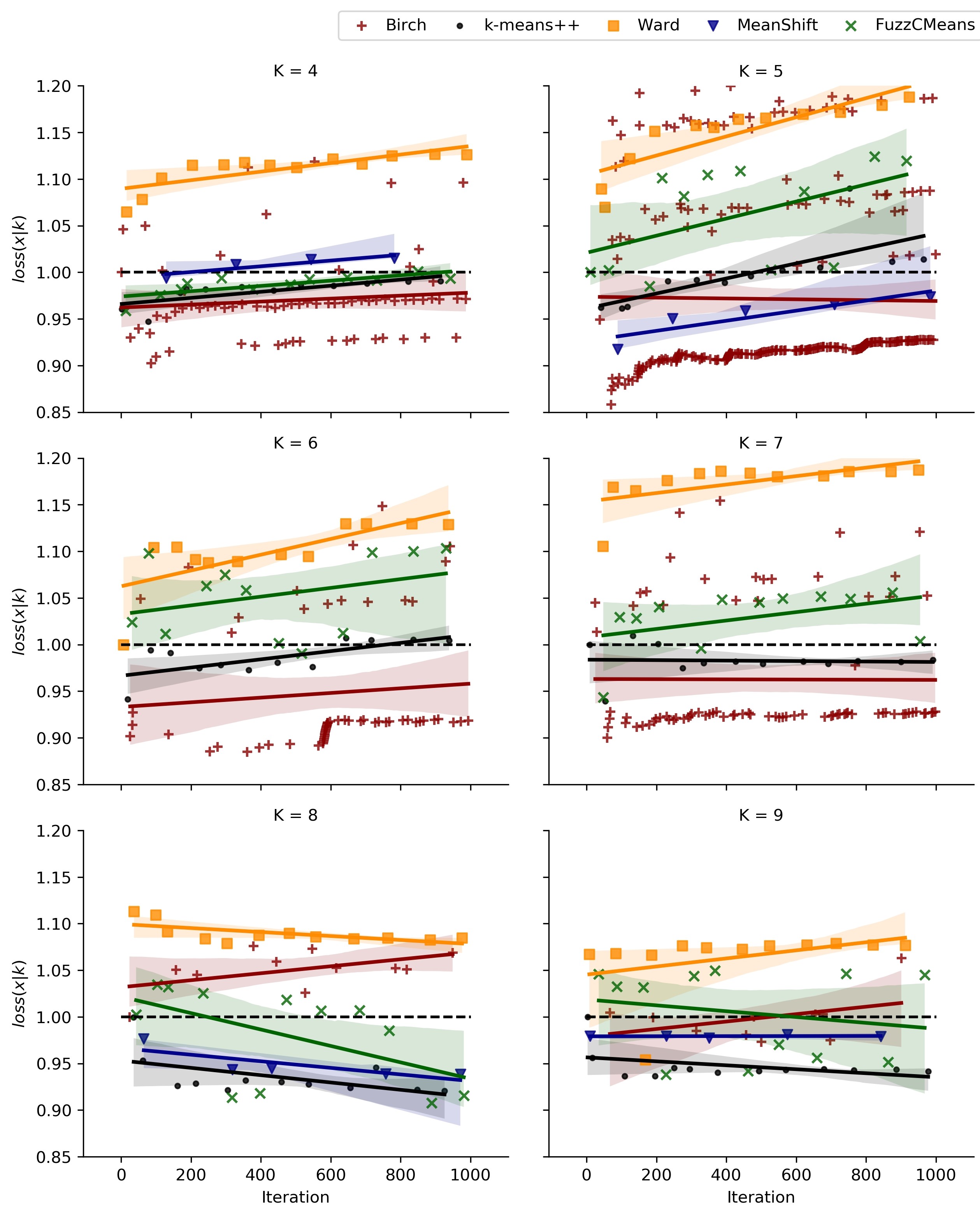
Figure 5: Bayesian-based clustering auto-tuning.

TABLE VII: Optimised clustering results and models

$k$	Algorithm	$bSI$	$\sigma(S_{k})$	$n$. boundary samples	$loss(x|k)$	$loss(x)$	$loss(k)$	Iteration	Hyperparameters
3	Birch	0.591	0.181	74	0.908	0.499	0.550	433	Branching factor: 50; Threshold: 0.2
4	k-means++	0.554	0.235	71	0.986	0.564	0.572	608	Type: Elka; n:1
5	MeanShift	0.541	0.213	75	0.917	0.565	0.616	89	Quantile:0.4
6	Birch	0.535	0.202	76	0.908	0.566	0.623	585	Branching factor: 50; Threshold: 0.4
7	Birch	0.501	0.200	85	0.928	0.598	0.645	998	Branching factor: 80; Threshold: 0.4
8	FuzzCMeans	0.448	0.200	128	0.908	0.652	0.718	889	m:1.8
9	FuzzCMeans	0.441	0.204	96	0.944	0.661	0.701	887	m:1.2

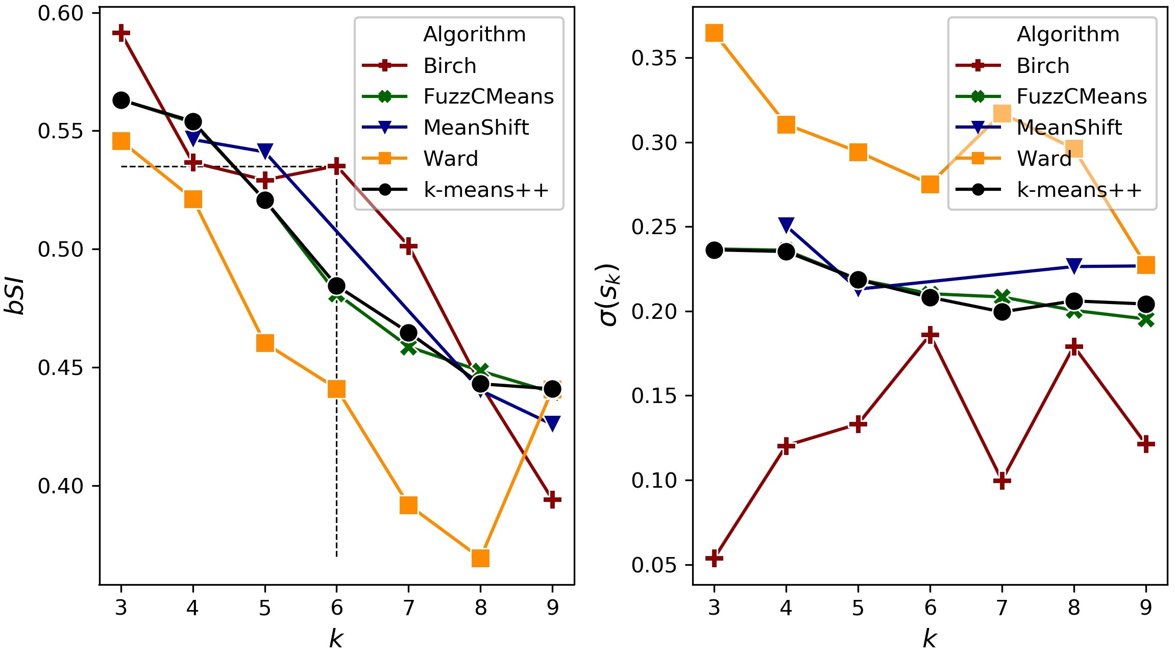
Figure 6: Performance comparison of the best settings of each algorithm.

IV-C3 Algorithm Heterogeneity Analysis

Different clustering algorithms present diverse characteristics in the hyperparameter auto-tuning process. The heterogeneity is summarised based on $bSI$ by a letter-value plot in Fig. 7. Letter-value plots display further letter values than Boxplots (i.e., display the median and quartiles only), which include more detailed information about the tails behaviour and afford more precise estimates of corresponding quantiles, thus are more appropriate for imbalanced data.

From Fig. 7, it is found that: (1) the k-means++ and Ward tend to have stable results with different hyperparameter values, which implies they are more straightforward to use without sophisticated tuning, and (2) hyperparameter tuning has a greater impact on the performance of Birch and Fuzzy C means, which implies that the benefit is better results; meanwhile, without sophisticated tuning, worse results than k-means++ are likely to be obtained. Autocluster enables a straightforward framework to generate better clustering quality and hyperparameter values by automatic iterative optimisation.

Besides, clustering ensemble presents a better overall performance in favour over the best stand-alone model, in both reliability and robustness. The end result can be constructed by a consensus function of majority voting, which iteratively adds the clustered labels generated by promising algorithms, and majority labels are specified as the final results. The decision boundary of the clustering ensemble is better and more convincing, even in the presence of noise and outlier points, on average. Nevertheless, these benefits come at a price, such as computation costs and complicated outputs interpretation.

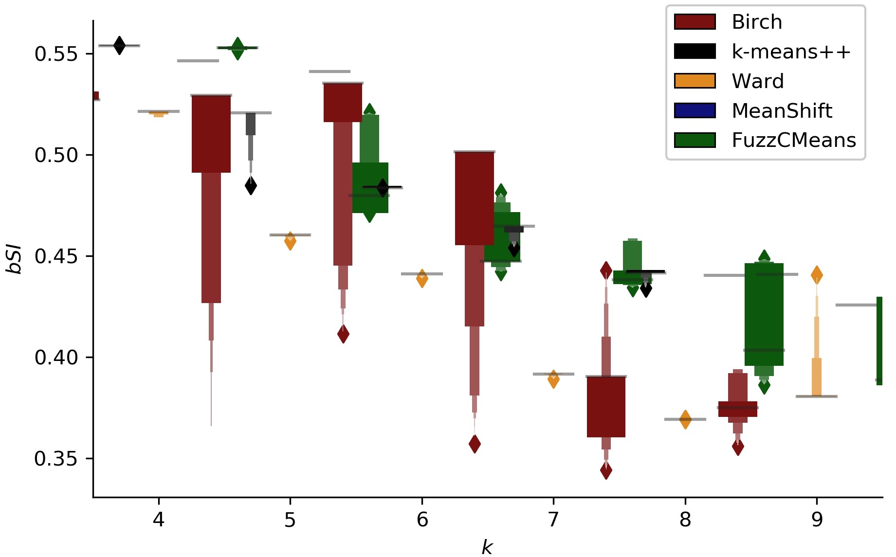
Figure 7: Algorithm heterogeneity analysis.

IV-D Risk Decoding and Data Labelling

IV-D1 Optimal Number of Clusters

The Autocluster also contributes in determining an optimal number of clusters ($k$) without $a~{}priori$ knowledge. Hierarchical risk partitions formed by incremental $k$ are illustrated in Fig. 8. The Sankey diagram emphasises the flows of instances across different clusters based on the corresponding risk levels. Widths of the bands are linearly proportional to the total number of samples clustered into each risk level.

With the increase of $k$, the retrieval resolution of cluster partitions is increased, which facilitates to separate more minority cases from the majority, thus the highest risk levels are uncovered. Meanwhile, a larger $k$ will encounter more instances that are placed in boundaries (as listed in TABLE VII or mis-clustered (as indicated by $Sample~{}Silhouette<0.05$, in Fig. 4). The clustering results with the best performance for each $k$ are auto-configured; however, the performance across different $k$ is not directly comparable.

The trade-offs between cluster quality and retrieval resolutions are illustrated in Fig. 6. The elbow point suggests the partition of $k=6$ is better clustered. Moreover, based on sample $s(i)$, Silhouette analysis is conducted to further investigate the detailed separation distance and density between the formed clusters, as illustrated in Fig. 9. The total number in each cluster can be visualised from the thickness of the silhouette plot. Positive $s(i)$ values indicate that the samples have been assigned to the right cluster.

The Silhouette plot provides a succinct graphical representation of how well each data point has been clustered. With reference to $bSI$ and $\sigma(S_{k})$ the performance of minority clusters is consistent with the majority. In comparison, it is better than the results commonly presented in imbalanced clustering (e.g., an obvious quality fluctuation among the minority and majority). The Silhouette plot further supports the results of Autocluster being reliable and of high-quality.

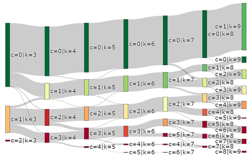
Figure 8: Hierarchical risk partitions and clustering flows by Autocluster.

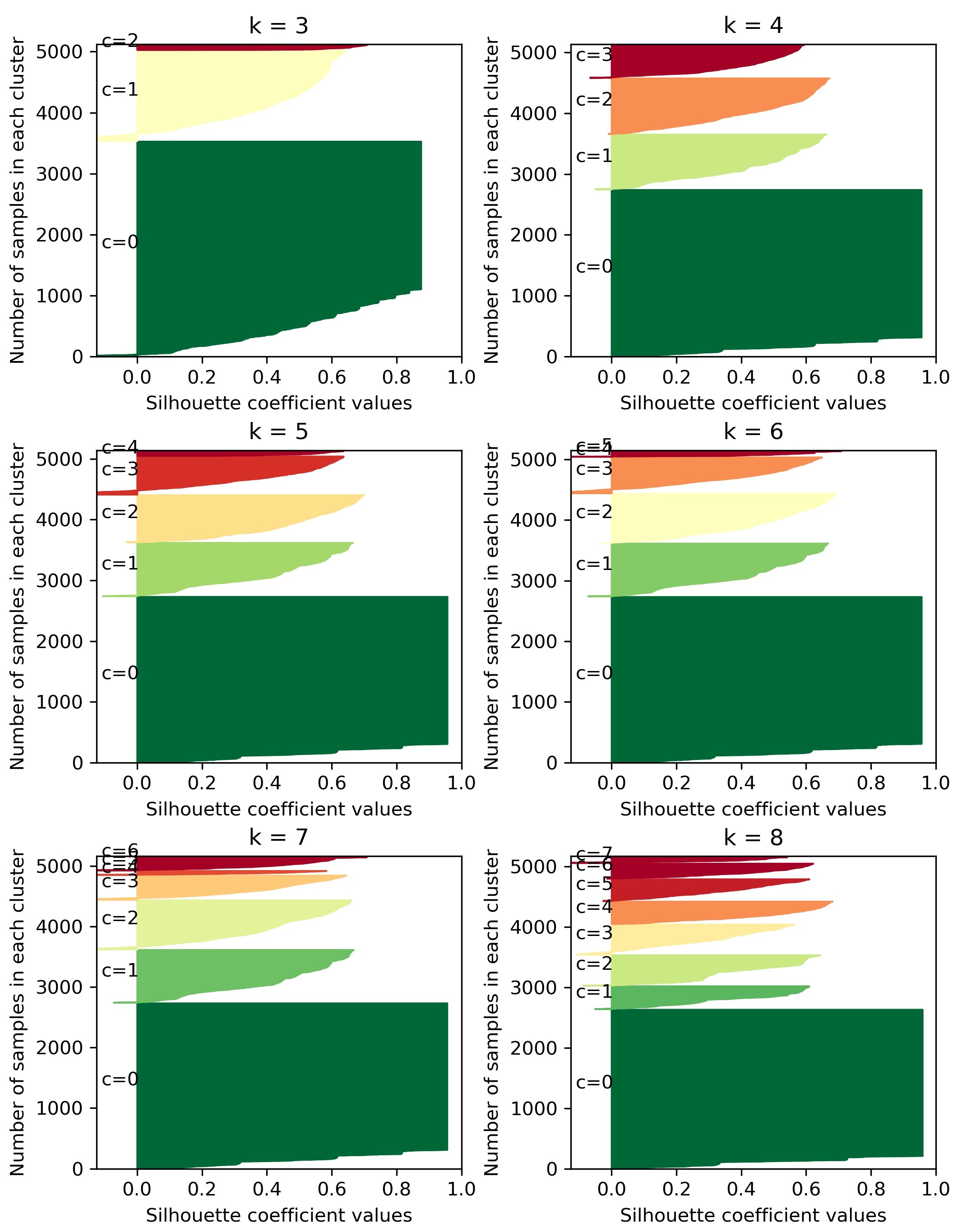
Figure 9: Silhouette analysis for clustering evaluation from the sample data level.

IV-D2 Risk Pattern Decoding

Vehicles with similar feature patterns are grouped into the same cluster, and each cluster has a respective distinct risk pattern. The key risk indicator features are selected based on EMRI, which can facilitate to recognise and interpret the risk patterns of the formed clusters, thus the labels of risk levels to each vehicle can be assigned. The value distributions of the key features are summarised in Fig. 10 based on letter-value plots. Based on the value and physical meanings of indictor features, the risk pattern can be decoded with graded levels from safety to the highest severity.

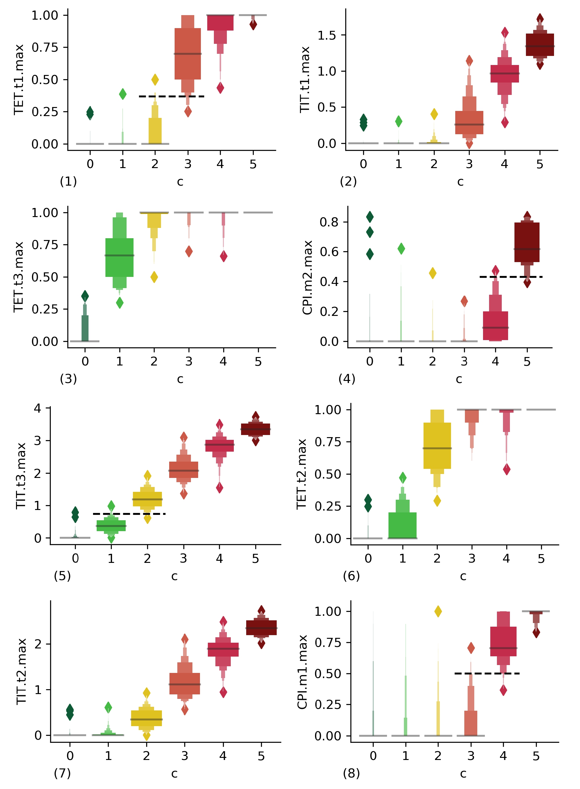
Figure 10: Indicator feature value distribution for risk level decoding.

IV-D3 Unsupervised Data Labelling

The clustering captures the position (i.e., the risk level) of a data instance in the entire dataset based on multidimensional views of feature similarity, and a label about the belonged position can be assigned to the instance. Herein, according to the above risk pattern interpretation and physical meanings of indictors, 6 risk levels can be defined. One annotation can be: safe level ($c=0$; with $2,725$ instances, about $53.6\%$ of total data; $indicators=0$), 3 risk levels from low to moderate ($c=1,2,3$; with instances of $872,810,591$, respectively; based on $TET~{}or~{}TIT>0$ with different thresholds sensitivity), and 2 high-risk levels ($c=4,5$; with $66$ and $18$ instances, respectively; based on $CPI>0$). The safe level indicates the lowest likelihood to be involved in vehicle crashes, and vice versa. Besides, an imbalance ratio ($IR$) is commonly used to measure the class imbalance, which is defined as the ratio of the number of instances in the majority class to the number of the minority class instances [18]. A dataset is referred to as highly imbalanced if the $IR$ is greater than 9. Herein, the $IR$ is 32 in our dataset, calculated by $2,725/(66+18)$.

TABLE VIII: Hybrid indicators and thresholds for risk estimation

	Risk levels	$Mean$	$Std$	($Min$, $Max$)	Threshold value
$TIT.t3.max$	$c=1\mid c=2$	0.38 $\mid$ 1.20	0.21 $\mid$ 0.28	(0.05, 0.74) $\mid$ (0.73, 1.74)	0.74
$TET.t1.max$	$c=2\mid c=3$	0.05 $\mid$ 0.69	0.11 $\mid$ 0.22	(0, 0.37) $\mid$ (0.30, 1.0)	0.37
$CPI.m1.max$	$c=3\mid c=4$	0.06 $\mid$ 0.74	0.14 $\mid$ 0.16	(0, 0.50) $\mid$ (0.49, 1.0)	0.50
$CPI.m2.max$	$c=4\mid c=5$	0.13 $\mid$ 0.65	0.14 $\mid$ 0.15	(0, 0.44) $\mid$ (0.41, 0.83)	0.44

IV-E Learning-based Risk Profiling

IV-E1 Hybrid Indicators for Risk Estimation with Threshold Calibrated by Clustering

The risk auto-clustering generates the optimised partitions based on risk indicator features, which is an unsupervised way to calibrate the threshold values of indicators. As highlighted by dashed horizontal lines in Fig. 10, 4 indicator features (i.e., $TIT.t3.max$, $TET.t1.max$, $CPI.m1.max$, $CPI.m2.max$) are obviously better in terms of differentiating certain adjacent risk levels by simplified decision rules and thresholds, e.g., less overlapping. The 4 indicators and thresholds for risk estimation are listed in TABLE VIII, which are calibrated by clustering based on big data and unsupervised feature selection.

The 4 indicators are therefore suitable to be used as key risk signals to estimate risk potentials. Besides, $CPI$-based indicators show the ability to well isolate the higher risk levels, which is in line with their physical meanings. For multiple risk assessment, hybrid use of indicators with simplified thresholds is useful in many application scenarios (e.g., limited computation capacity, insufficient data), which is also better than relying on one stand-alone indicator with over-complicated threshold values. Besides, risk levels defined by hybrid indicators with straightforward thresholds are interpretable and easy to adopt by end-users.

IV-E2 High-resolution Dynamic Risk Profiling

The driving risks and anomaly behaviour of a vehicle can be inferred based on the risk patterns of the belonged cluster accordingly under the smart road environment. A high-resolution risk profiling is demonstrated in Fig. 11, in which two lanes are selected to demonstrate the microscopic risk exposures inherent in generalised traffic flow, such as the at-risk vehicles, risk severity, distribution, trends. In the plots, the $x-axis$ denotes the timestamps, in sub-second interval ($0.1s$), and the $y-axis$ denotes the travelled distance or locations on each lane, in metre-scale.

The vehicle trajectory time-series data is integrated with dynamic risk levels, hence, target vehicles with risk potentials can be figured out, thus the locations and times with higher risk potentials can also be identified. The granular risk profiling is more meaningful and useful to early identify potential crashes, and take targeted countermeasures for mitigation. In real-world applications, the data can be collected by multiple manners, such as roadside sensing, surveillance cameras, connected vehicle system, etc.

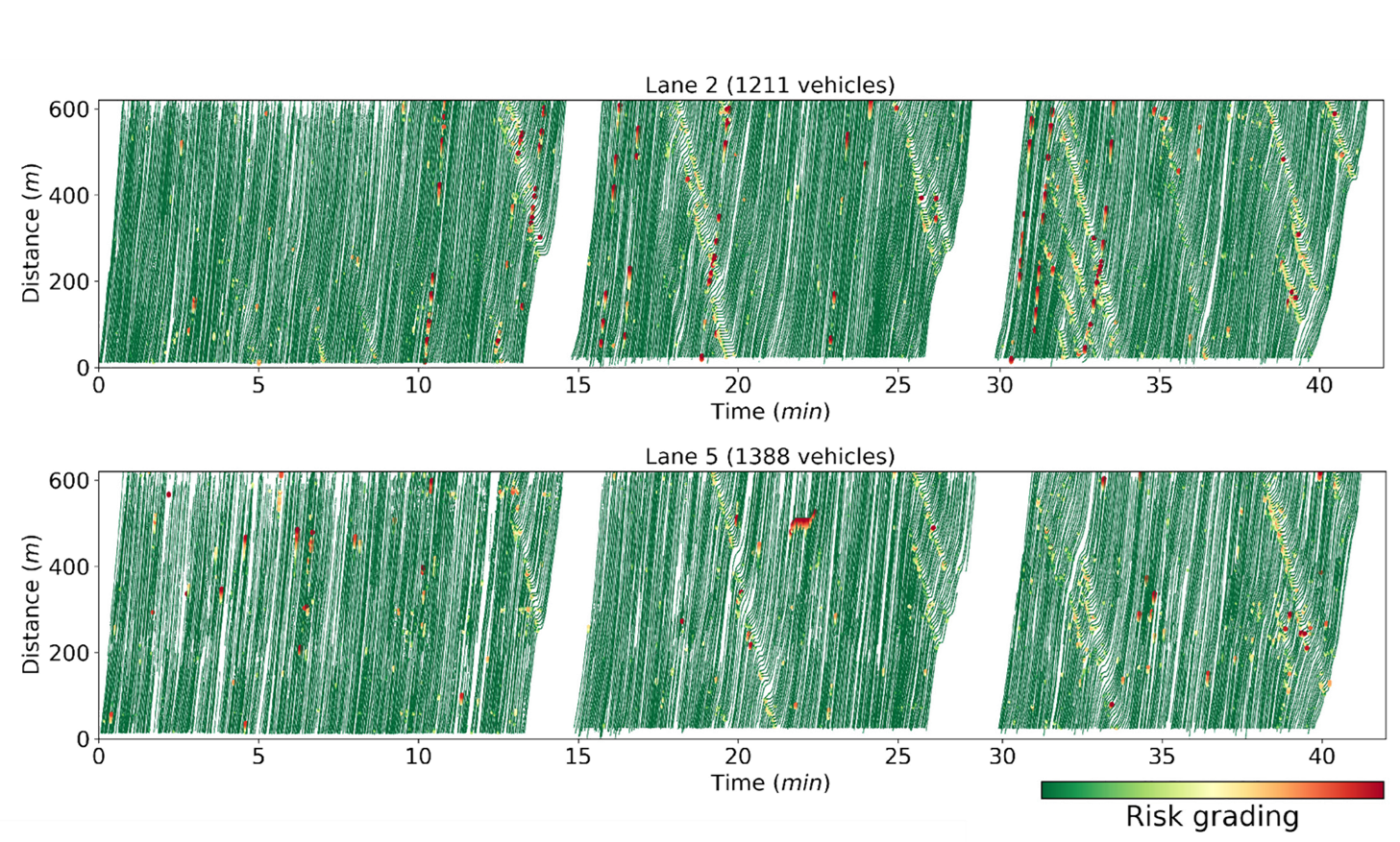
Figure 11: High-resolution dynamic risk detection and profiling.

V Discussion

V-A Limitations and Future Work

Risk diagnosis by Autocluster enables a predictive and proactive manner towards smart safety, which is prospected to identify and mark early risk signals and at-risk vehicles. However, result verification is a major challenge. A potential way of validation is to examine the actual crash occurrence, or the insurance claim records of the drivers/vehicles clustered to be of higher risk, which requires another way of data acquisition.

To further improve modelling, in-depth extraction of indicator features and using high-quality data are suggested, which may involve a broader range of risk potentials and driving scenarios, such as lane changing. Methodologically, new algorithms on clustering and AutoML can be integrated to refine the solution.

In view of a large number of real-world applications suffering from the challenges of class imbalance and lack of ground truth (e.g., expensive or difficult to obtain beforehand), we demonstrate a reliable solution with a case on road safety, which holds great potentials.

V-B Application Potentials

The data mining about risk exposures is clearly an area with huge values-add and also a core concern of CAV and smart road. The application potentials are multiple folds. For roads and authorities, protective and pre-crash strategies can be applied pre-emptively, such as patrol despatch, flow control, road enhancement (e.g. remediation of crash-prone layouts and locations), which extends the scope of traditional policy-making and management (e.g., passive and post-accident). For vehicles and drivers, advance driver-assistance services can be provided, such as risk warnings and driving recommendations (e.g. re-routing or lane-changing to avoid road segments or lanes with risk potentials).

VI Conclusions

The indicator-guided automatic clustering is reliable and convincing, to end-to-end self-learn the optimal models for unsupervised risk assessment and driving anomaly detection. The developed methods are useful towards a range of advanced solutions towards smart road and crash prevention, and to tackle intrinsic challenges of clustering on highly imbalanced data without ground truth labels or $a~{}priori$ knowledge. In summary, this research has contributed to the domain knowledge in four areas, as highlighted in the following.

(1) Multiple risk levels in generalised driving. The Autocluster aims to diagnose multiple distinct risk exposures inherent to generalised driving behaviour as exhibited by the vehicle stream trajectory, which is also a method of unsupervised data labelling. It is an attempt to uncover the risk exposure levels in normal traffic conditions, which extends the scope of risk analysis as relying on accidents. The method is tested on NGSIM data, and a clustering with 6 distinct risk levels is generated, as well as the risk labels per vehicle.

(2) The Autocluster system. Autocluster enables the auto-optimisation of risk clustering adapted onto data. Various notions of clustering algorithms and similarity measures are tested. A loss function is designed that considers the clustering performance in terms of internal quality, inter-cluster variation, and model stability. Based on Bayesian optimisation, the algorithm selection and hyperparameter tuning are self-learned, and the best risk clustering partitions with the minimum loss are generated. The performance and heterogeneity of various algorithms are also analysed.

(3) Strategies to improve imbalanced clustering. Firstly, an internal quality metric for imbalanced clustering is proposed, namely $bSI$, which is demonstrated to be more appropriate than existing CVIs. Secondly, an unsupervised feature selection method, namely EMRI, is proposed to identify the most useful features for the clustering problem. Besides, feature rectifier function is designed as a cost-sensitive strategy to improve imbalanced clustering.

(4) Learning-based risk profiling. The surrogate indicators on temporal-spatial and kinematical risk exposures are evaluated by unsupervised feature selection and ranking, and $TIT$, $TET$ and $CPI$ are found to be more useful for risk assessment. Multiple thresholds of risk indicators are benchmarked by Autocluster. In addition, high-resolution risk detection and positioning are delineated to figure out the risk potentials in terms of targeted vehicles, locations in metre-scale, and timestamps in the sub-second interval, which enable a range of application potentials for the smart road.

References

- [1] A. Eskandarian, C. Wu, and C. Sun, “Research advances and challenges of autonomous and connected ground vehicles,” IEEE Transactions on Intelligent Transportation Systems, 2019.
- [2] S. Mozaffari, O. Y. Al-Jarrah, M. Dianati, P. Jennings, and A. Mouzakitis, “Deep learning-based vehicle behavior prediction for autonomous driving applications: A review,” IEEE Transactions on Intelligent Transportation Systems, pp. 1–15, 2020.
- [3] L. Zhu, F. R. Yu, Y. Wang, B. Ning, and T. Tang, “Big data analytics in intelligent transportation systems: A survey,” IEEE Transactions on Intelligent Transportation Systems, vol. 20, no. 1, pp. 383–398, 2018.
- [4] D. Nallaperuma, R. Nawaratne, T. Bandaragoda, A. Adikari, S. Nguyen, T. Kempitiya, D. De Silva, D. Alahakoon, and D. Pothuhera, “Online incremental machine learning platform for big data-driven smart traffic management,” IEEE Transactions on Intelligent Transportation Systems, vol. 20, no. 12, pp. 4679–4690, 2019.
- [5] X. Shi, Y. D. Wong, M. Z.-F. Li, C. Palanisamy, and C. Chai, “A feature learning approach based on xgboost for driving assessment and risk prediction,” Accident Analysis and Prevention, vol. 129, pp. 170–179, 2019.
- [6] X. Shi, Y. D. Wong, C. Chai, and M. Z.-F. Li, “An automated machine learning (automl) method of risk prediction for decision-making of autonomous vehicles,” IEEE Transactions on Intelligent Transportation Systems, 2020.
- [7] X. Shi, Y. D. Wong, M. Z. F. Li, and C. Chai, “Key risk indicators for accident assessment conditioned on pre-crash vehicle trajectory,” Accident Analysis and Prevention, vol. 117, pp. 346–356, 2018.
- [8] C. Chai and Y. D. Wong, “Fuzzy cellular automata model for signalized intersections,” Computer-Aided Civil and Infrastructure Engineering, vol. 30, no. 12, pp. 951–964, 2015.
- [9] C. Chai and Y. Wong, “Micro-simulation of vehicle conflicts involving right-turn vehicles at signalized intersections based on cellular automata,” Accident Analysis and Prevention, vol. 63, pp. 94–103, 2014.
- [10] M. A. Perez, J. D. Sudweeks, E. Sears, J. Antin, S. Lee, J. M. Hankey, and T. A. Dingus, “Performance of basic kinematic thresholds in the identification of crash and near-crash events within naturalistic driving data,” Accident Analysis and Prevention, vol. 103, pp. 10–19, 2017.
- [11] M. Siami, M. Naderpour, and J. Lu, “A mobile telematics pattern recognition framework for driving behavior extraction,” IEEE Transactions on Intelligent Transportation Systems, pp. 1–14, 2020.
- [12] L. Zheng, K. Ismail, and X. Meng, “Traffic conflict techniques for road safety analysis: Open questions and some insights,” Canadian Journal of Civil Engineering, vol. 41, no. 7, pp. 633–641, 2014.
- [13] S. S. Mahmud, L. Ferreira, M. S. Hoque, and A. Tavassoli, “Application of proximal surrogate indicators for safety evaluation: A review of recent developments and research needs,” IATSS Research, vol. 41, no. 4, pp. 153–163, 2017.
- [14] A. Laureshyn, Å. Svensson, and C. Hydén, “Evaluation of traffic safety, based on micro-level behavioural data: Theoretical framework and first implementation,” Accident Analysis and Prevention, vol. 42, no. 6, pp. 1637–1646, 2010.
- [15] V. Estivill-Castro, “Why so many clustering algorithms,” ACM SIGKDD Explorations Newsletter, vol. 4, no. 1, pp. 65–75, 2002.
- [16] A. Rodriguez and A. Laio, “Clustering by fast search and find of density peaks,” Science, vol. 344, no. 6191, pp. 1492–1496, 2014.
- [17] C. Elkan, “The foundations of cost-sensitive learning,” in International Joint Conference on Artificial Intelligence, vol. 17, no. 1, 2001, pp. 973–978.
- [18] J. F. Díez-Pastor, J. J. Rodríguez, I. García-Osorio, and I. Kuncheva, “Diversity techniques improve the performance of the best imbalance learning ensembles,” Information Sciences, vol. 325, pp. 98–117, 2015.
- [19] C. Beyan and R. Fisher, “Classifying imbalanced data sets using similarity based hierarchical decomposition,” Pattern Recognition, vol. 48, no. 5, pp. 1653–1672, 2015.
- [20] V. López, A. Fernández, S. García, V. Palade, and F. Herrera, “An insight into classification with imbalanced data: Empirical results and current trends on using data intrinsic characteristics,” Information Sciences, vol. 250, pp. 113–141, 2013.
- [21] R. C. de Amorim and C. Hennig, “Recovering the number of clusters in data sets with noise features using feature rescaling factors,” Information Sciences, vol. 324, pp. 126–145, 2015.
- [22] T. van Craenendonck and H. Blockeel, “Using internal validity measures to compare clustering algorithms,” Journal of Computational and Applied Mathematics, pp. 1–8, 2015.
- [23] M. Feurer, A. Klein, K. Eggensperger, J. Springenberg, M. Blum, and F. Hutter, “Efficient and robust automated machine learning,” in Advances in Neural Information Processing Systems, 2015, pp. 2962–2970.
- [24] B. Shahriari, K. Swersky, Z. Wang, R. P. Adams, and N. De Freitas, “Taking the human out of the loop: A review of bayesian optimization,” Proceedings of the IEEE, vol. 104, no. 1, pp. 148–175, 2015.
- [25] J. Snoek, H. Larochelle, and R. P. Adams, “Practical bayesian optimization of machine learning algorithms,” in Advances in Neural Information Processing Systems, 2012, pp. 2951–2959.
- [26] J. S. Bergstra, R. Bardenet, Y. Bengio, and B. Kégl, “Algorithms for hyper-parameter optimization,” in Advances in Neural Information Processing Systems, 2011, pp. 2546–2554.
- [27] P. J. Rousseeuw, “Silhouettes: a graphical aid to the interpretation and validation of cluster analysis,” Journal of Computational and Applied Mathematics, vol. 20, pp. 53–65, 1987.
- [28] O. Bousquet and A. Elisseeff, “Stability and generalization,” Journal of Machine Learning Research, vol. 2, pp. 499–526, 2002.
- [29] I. Guyon and A. Elisseeff, “An introduction to variable and feature selection,” Journal of Machine Learning Research, vol. 3, pp. 1157–1182, 2003.
- [30] A. van der Horst, “A time-based analysis of road user behaviour in normal and critical encounters,” Ph.D. dissertation, Delft University of Technology, 1990.
- [31] M. M. Minderhoud and P. H. Bovy, “Extended time-to-collision measures for road traffic safety assessment,” Accident Analysis and Prevention, vol. 33, no. 1, pp. 89–97, 2001.
- [32] J. Archer, “Indicators for traffic safety assessment and prediction and their application in micro-simulation modelling: A study of urban and suburban intersections,” Ph.D. dissertation, KTH, 2005.
- [33] F. Cunto and F. F. Saccomanno, “Calibration and validation of simulated vehicle safety performance at signalized intersections,” Accident Analysis and Prevention, vol. 40, no. 3, pp. 1171–1179, 2008.
- [34] A. Zarshenas and K. Suzuki, “Binary coordinate ascent: An efficient optimization technique for feature subset selection for machine learning,” Knowledge-Based Systems, vol. 110, pp. 191–201, 2016.
- [35] A. Fisher, C. Rudin, and F. Dominici, “All models are wrong, but many are useful: Learning a variable’s importance by studying an entire class of prediction models simultaneously,” Journal of Machine Learning Research, vol. 20, no. 177, pp. 1–81, 2019.
- [36] J. Halkias and J. Colyar, “Next generation simulation fact sheet,” US Department of Transportation: Federal Highway Administration, 2006.
- [37] V. Punzo, M. T. Borzacchiello, and B. Ciuffo, “On the assessment of vehicle trajectory data accuracy and application to the next generation simulation (ngsim) program data,” Transportation Research Part C: Emerging Technologies, vol. 19, no. 6, pp. 1243–1262, 2011.