Quantum chaos driven by long-range waveguide-mediated interactions

Abstract

We study theoretically quantum states of a pair of photons interacting with a finite periodic array of two-level atoms in a waveguide. Our calculation reveals two-polariton eigenstates that have a highly irregular wave-function in real space. This indicates the Bethe ansatz breakdown and the onset of quantum chaos, in stark contrast to the conventional integrable problem of two interacting bosons in a box. We identify the long-range waveguide-mediated coupling between the atoms as the key ingredient of chaos and nonintegrability. Our results provide new insights in the interplay between order, chaos and localization in many-body quantum systems and can be tested in state-of-the-art setups of waveguide quantum electrodynamics.

Introduction. Arrays of superconducting qubits or cold atoms coupled to a waveguide, have recently become a promising new platform for quantum optics Roy et al. (2017); Chang et al. (2018); van Loo et al. (2013); Corzo et al. (2019); Mirhosseini et al. (2019); Brehm et al. (2020); Prasad et al. (2020). They can be used for storing  Leung and Sanders (2012) and generating quantum light Zheng et al. (2013); Zheng and Baranger (2013); Johnson et al. (2019); Prasad et al. (2020), and even a future “quantum internet” Kimble (2008). Moreover, qubit arrays are a new type of quantum simulator for the problems of many-body physics Noh and Angelakis (2016); Xu et al. (2018); Iorsh et al. (2020). One of the most fundamental problems in physics is the competition between order and chaos, or many-body localization and thermalization. It is already a subject of active studies Faddeev (2013); Moore (2017), from celestial mechanics to atomic, nuclear Bunakov (2016) and condensed matter  Ullmo (2008); D’Alessio et al. (2016); Aßmann et al. (2016) physics, and even quantum paradoxes in black holes Maldacena et al. (2016); Morita (2019). Despite the large diversity of these systems, the consideration is typically limited to excitations with parabolic dispersions and short-range coupling. Arrays of atoms in a waveguide present a unique platform to probe unexplored boundaries of quantum chaos and integrability. They offer a special combination of strong interactions, long-range waveguide-mediated coupling and intrinsically non-parabolic dispersion of excitations.

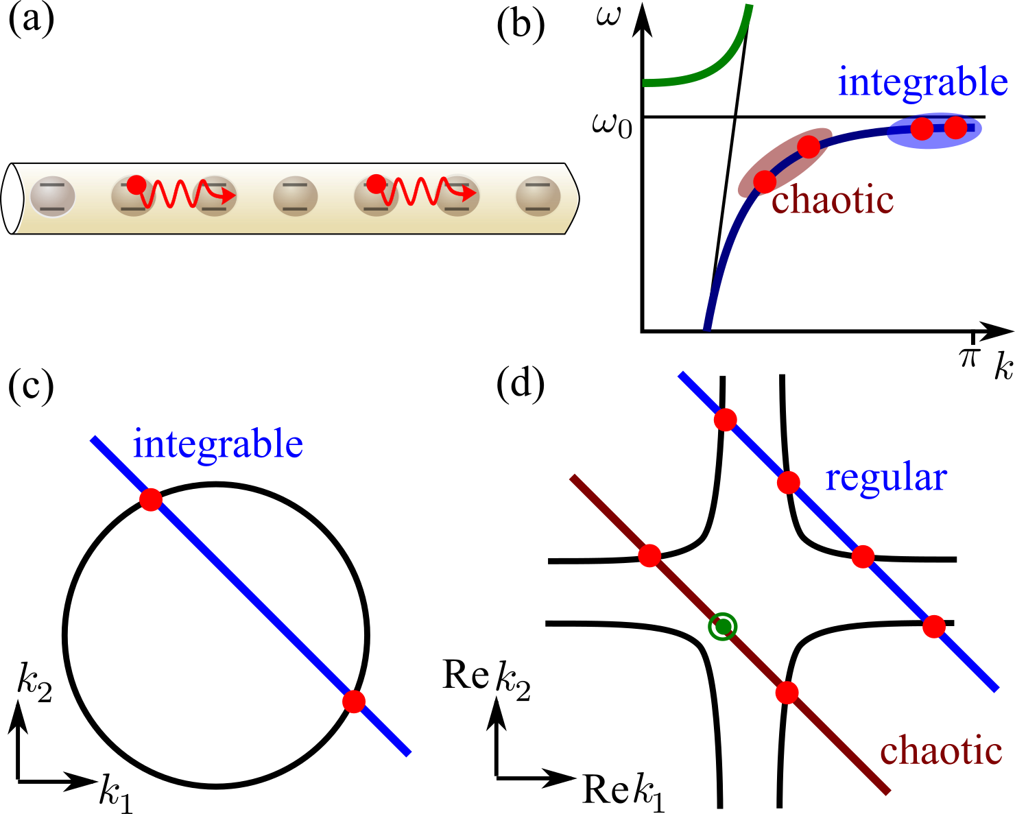
Figure 1: (a) Schematics of a two-photon state in array of atoms in a waveguide. (b) Schematics of single-polariton dispersion curve $\omega(k)$. Two polaritons pairs with small and large wave vectors corresponding to chaotic and integrable states are indicated. (c,d) Wave vectors of two-polariton states with the same total energy and momentum for the case of (c) parabolic and (d) non-parabolic $\propto-1/k^{2}$ single-particle dispersion. Black curves shows the isoenergy contour $\omega(k_{1})+\omega(k_{2})=const$. Slanted lines illustrate the total momentum conservation, $k_{1}+k_{2}=const$. Green circle in (c) corresponds to the complex $k_{1,2}$, with real part outside the isoenergy contour.

Here, we consider an interaction of two photons with a periodic finite array of two-level atoms in a waveguide, illustrated in Fig. 1(a). The coupling of photons to atoms leads to the formation of collective polaritonic excitations. Polaritons repel each other since a single two-level atom can not host two resonant photons at the same time Birnbaum et al. (2005). This is strongly reminiscent of an exactly solvable (integrable) one-dimensional model of two bosons in a box, that demonstrates fermionization in the limit of strong repulsion Lieb and Liniger (1963); McGuire (1964); Gaudin (1971). The integrability can be broken when the interaction becomes nonlocal Beims et al. (2007), or there is an external potential Shepelyansky (2016), or if the bosons acquire different masses Van Vessen et al. (2001), which can be mapped to an irrational-angle billiard  Casati and Prosen (1999). Since considered polaritons are locally interacting equivalent bosons and there is no external potential the integrability should persist at the first glance. Indeed, fermionized two-polariton states have been recently revealed by Zhang and Mølmer  Zhang and Mølmer (2019). However, we later uncovered Zhong et al. (2020); Poshakinskiy et al. (2020) a very different kind of two-polariton states that have a broad Fourier spectrum, and cannot be reduced to a product of several single-particle states. This hints that the problem is non-integrable by the Bethe ansatz. The mechanism of non-integrability and its possible consequences, such as existence of chaotic two-polariton states remain unclear.

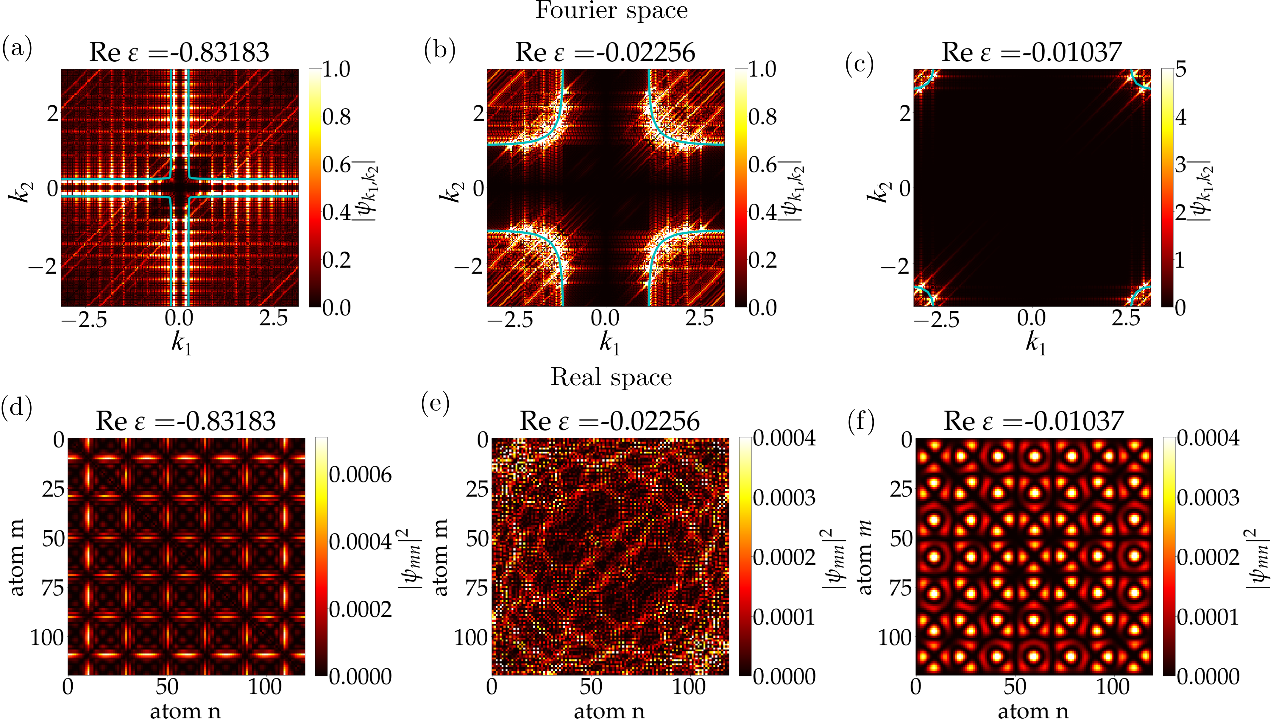
Figure 2: (a,b,c) Fourier transforms and (d,e,f) real-space wavefunctions of several characteristic two-polariton states. (a,d): regular nonintegrable state, (b,e): irregular chaotic-like state, (c,f): fermionized state. The calculation has been performed for $N=120$ qubits and $\varphi=0.02$. Cyan curves in (a–c) show the isoenergy contours Eq. (2). Energy is measured in units of $\Gamma_{0}$.

In this Letter, we examine the transition between the regular two-polariton states Zhong et al. (2020); Poshakinskiy et al. (2020) and the fermionized states Zhang and Mølmer (2019) and identify the emergence of chaotic two-polariton eigenstates at the transition point. In a nutshell, the origin of chaotic states can be understood by analyzing the conservation of energy $\omega(k_{1})+\omega(k_{2})=2\varepsilon$ and center of mass momentum $k_{1}+k_{2}=K$ for two interacting polaritons, as shown in Fig. 1(c,d). In a conventional system with parabolic dispersion $\omega\propto k^{2}$ there exist just two pairs of particles with given total energy $2\varepsilon$ and momentum $K$. These two pairs can be found from the intersection of the isoenergy curve $k_{1}^{2}+k_{2}^{2}=const$ [circle in Fig. 1(c)] with the iso-momentum line $k_{1}+k_{2}=const$ [blue line in Fig. 1(c)]. However, the dispersion of polaritons is strongly nonparabolic, resulting from avoided crossing of light dispersion $\omega(k)=ck$ with the atomic resonance at $\omega=\omega_{0}$, see Fig. 1(b) Ivchenko (1991); Albrecht et al. (2019); Zhong et al. (2020). Specifically, for the intermediate part of the lower polariton branch away from the Brillouin zone edge one has $\omega(k)\propto-1/k^{2}$ Zhong et al. (2020) and the isoenergy curve $\omega(k_{1})+\omega(k_{2})=const$ acquires a more complicated hyperbolic shape [Fig. 1(d)] instead of a circle in Fig. 1(c). There exist 4 pairs of polaritons with a given total energy and momentum [blue line in Fig. 1(d)] instead of 2 pairs in Fig. 1(c). Moreover, the values of $k_{1}$ and $k_{2}$ can be complex even when total momentum and energy are real [red line in Fig. 1(d)]. We prove below that the combination of polariton-polariton interactions with polariton reflections from the array edges, when $k_{1,2}\to-k_{1,2}$, makes the number of single-particle states with the same total energy and momentum arbitrarily large. We have found a chaotic nonlinear map that governs the distribution of wave vectors $k$ and thus drives chaotic two-polariton states. Such mechanism of emergence of chaos and nonintegrability is very general and should apply to various many-body setups with nonparabolic dispersion of excitations, that is typical for long-range coupling.

Regular and irregular two-photon states. We will now present details of the model and numerical results. We consider $N$ periodically spaced qubits in a one-dimensional waveguide, characterized in the Markovian approximation by the Hamiltonian $\mathcal{H}=\sum_{m,n=1}^{N}H_{m,n}b_{m}^{{\dagger}}b_{n}+\frac{\chi}{2}\sum_{n=1}^{N}b_{n}^{{\dagger}}b_{n}^{{\dagger}}b_{n}^{\vphantom{{\dagger}}}b_{n}^{\vphantom{{\dagger}}}\>,$ where $H_{mn}\equiv-{\rm i}\Gamma_{0}{\rm e}^{{\rm i}\varphi|m-n|}\>,\quad m,n=1\ldots N\>.$ Here, $b_{m}$ are the annihilation operators for the bosonic excitations of the qubits and $\varphi$ is the phase acquired by light between the two neighboring qubits. The details of derivation can be found in Refs. Caneva et al. (2015); Ke et al. (2019) and also in Supplementary Materials. The Hamiltonian is non-Hermitian due to the possibility of radiative losses into the waveguide and the coupling strength does not decay with distance. We consider subwavelength regime when $\varphi\sim 1/N\ll 1$. The parameter $\Gamma_{0}$ is the radiative decay rate of an individual qubit and the anharmonicity $\chi$ is responsible for polariton-polariton interactions. We focus on the double-excited states $\sum_{m,n}\psi_{mn}b_{n}^{\dagger}b_{m}^{\dagger}|0\rangle$. In the limit of two-level qubits, when $\chi/\Gamma_{0}\to\infty$ and $\psi_{nn}\equiv 0$, the Schrödinger equation for these states reads (see Refs. Ke et al. (2019); Zhong et al. (2020) and Supplementary Materials):

$$H_{nn^{\prime}}\psi_{n^{\prime}m}+\psi_{nn^{\prime}}H_{n^{\prime}m}-2\delta_{nm}H_{nn^{\prime}}\psi_{n^{\prime}n}=2\varepsilon\psi_{nm}\>,$$ (1)

with $\psi_{nm}=\psi_{mn}$, and $n,m=1\ldots N$. Here, the first two terms in the left-hand side describe the propagation of the first and second polaritons, respectively. The third term accounts for their repulsion, enforcing $\psi_{nn}=0$.

Figure 2 presents three characteristic eigenstates, with the energies increasing from left to right, calculated numerically for an array with $N=120$ qubits. Top row shows two-dimensional Fourier transforms $|\sum_{nm}\psi_{nm}{\rm e}^{-{\rm i}k_{x}n-{\rm i}k_{x}m}|^{2}$ and the bottom row presents the real-space probability densities $|\psi_{nm}|^{2}$. The state in Fig. 2(a,d) can be understood from the analytical model where each one of the two polaritons induces in real space an effective periodic potential for the other one Poshakinskiy et al. (2020). It has a regular structure with sharp localized features in real space, Fig. 2(d) and a relatively broad distribution in the Fourier space with many discrete peaks concentrated along the isoenergy contour of non-interacting polariton pair Zhong et al. (2020),

$$\frac{\Gamma_{0}\sin\varphi}{\cos k_{1}-\cos\varphi}+\frac{\Gamma_{0}\sin\varphi}{\cos k_{2}-\cos\varphi}=2\varepsilon\>,$$ (2)

shown by the cyan curves in Fig. 2(a–c). As such, the state in Fig. 2(a,d) consists of many single-particle states and clearly cannot be described by a simple Bethe ansatz, although it has a regular real-space wavefunction. The state in Fig. 2(b,e) is very different and we will term it as a chaotic state. While it is hard to give a mathematically precise definition of chaotic states in a finite discrete system, we stress that the state Fig. 2(b) has a highly irregular wavefunction in real space, and, at the same time its Fourier spectrum in Fig. 2(e) is broad and relatively homogeneous along the isoenergy contour. This is in accordance with the Berry hypothesis for chaotic states Berry (1977). Finally, in Fig. 2(c,d) we show the fermionized two-polariton state Zhang and Mølmer (2019). The state is regular in real space, has 8 distinct peaks in the Fourier space, and is well described by the Bethe ansatz

$$\psi_{nm}=\psi_{mn}\propto \cos k_{1}(n-\tfrac{1}{2})\cos k_{2}(m-\tfrac{1}{2})$$ (3)

$$- \cos k_{2}(n-\tfrac{1}{2})\cos k_{1}(m-\tfrac{1}{2})\quad\text{for $n>m$. }$$

The coexistence of the fermionized regular eigenstates Fig. 2(c,f) with regular eigenstates Fig. 2(a,d) and chaotic eigenstates Fig. 2(b,e) for the same Hamiltonian and the same parameters is rather surprising. Our central goal is to explain this result and to identify the origin of the apparent chaotic character of the wavefunction Fig. 2(b,e).

Bethe ansatz and its breakdown. We first construct the Bethe ansatz solution for an infinite array and then explain where it fails for a finite array. It is inconvenient to start directly from the Schrödinger equation (1) since the corresponding Hamiltonian matrix is dense, i.e., includes long-range waveguide-mediated couplings. Instead, we use the fact that the inverse matrix $H^{-1}$ is tri-diagonal, and change the basis as $\psi=H^{-1}\Psi H^{-1}$ Poddubny (2020) to obtain an equivalent sparse equation Zhong et al. (2020)

$$(H^{-1}\Psi+\Psi H^{-1})_{nm}- 2\delta_{nm}(\Psi H^{-1})_{nn}$$

$$=2\varepsilon(H^{-1}\Psi H^{-1})_{nm}\>.$$ (4)

We now try to solve it using a Bethe ansatz

$$\Psi_{mn}=\sum_{K,q}A_{K,q}\,{\rm e}^{{\rm i}K(m+n)+{\rm i}q|m-n|/2}$$ (5)

where $A_{K,q}$ are the coefficients and the summation goes over particular values of the center of mass motion wave vector $K=(k_{1}+k_{2})/2$ and the relative motion wave vector $q=k_{1}-k_{2}$ that are determined below. Each term of the ansatz Eq. (5) shall satisfy Eq. (Quantum chaos driven by long-range waveguide-mediated interactions) at all $m,n$ except for the diagonal region $|m-n|=0,1$ and the array boundaries $m,n=1,N$. That is fulfilled if $k_{1,2}=K\pm q/2$ lies on the isoenergy contour Eq. (2).

First, we consider an infinite array, where the center of mass wave vector $K$ is a good quantum number. Substituting $k_{1,2}=K\pm q/2$ in the dispersion equation Eq. (2) we find 4 inequivalent values of the relative motion wave vector $q(K)$ for any value of $K$. The values of $q$ can be both real and complex, explicit expressions are given in the Supplementary Materials. Real-valued solutions can be found from the intersection of the line $k_{1}+k_{2}=K$, describing all states with given total momentum, with the isoenergy contour Eq. (2), see Fig. 1(d). These four solutions can be combined in Eq. (5) to satisfy Eq. (Quantum chaos driven by long-range waveguide-mediated interactions) as shown in the Supplementary Materials which finishes the construction of the Bethe ansatz in the infinite system. However, this procedure breaks down for a finite array.

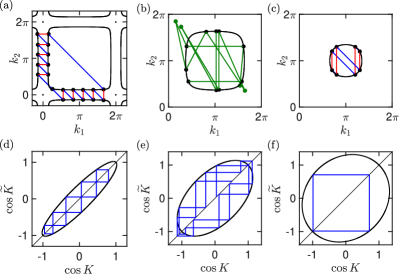
Figure 3: Examples of subsequent application of the map Eq. (6), for different initial wave vectors: (a) regular 21-cycle, starting with $k_{1}=0.8$, $k_{2}=0.5$, (b) ergodic infinite cycle starting with $k_{1}=1.33$, $k_{2}=1.73$, (c) 8-cycle in fermionic regime starting with $k_{1}=2.2$, $k_{2}=3.8$. Green points in (b) show real parts of complex wave vectors. For (b,c) the vectors $k_{1,2}$ are reduced to the Brillouin zone $0\leq k_{1,2}\leq 2\pi$ before the vector $K=(k_{1}+k_{2})/2$ is calculated. Black lines show the isofrequency contours Eq. (2). Bottom panels (d-f) show the same cycles as in (a-c) but plotted for the equivalent map Eq. (7), tracing the evolution of the center-of-mass wave vector $K$.

In a finite array, photons can reflect from the boundaries. To accommodate the boundaries, one should include in Bethe ansatz the reflected waves with the wave vectors $\widetilde{k}_{1,2}=-k_{1,2}$. After the reflection of one of the two photons, the new center of mass wave vector is $\widetilde{K}=(\widetilde{k}_{1}+\widetilde{k}_{2})/2=\pm(k_{1}-k_{2})/2=\pm q/2$. Thus, we obtain a nonlinear map

$$K\to\widetilde{K}=\pm\frac{1}{2}q(K)\>,$$ (6)

which generates new pairs of wave vectors $K$ and $q(K)$ that must be included into the Bethe ansatz Eq. (5). All the generated plane waves should be combined to satisfy the Schrödinger equation at the boundaries Batchelor (2007); Zhang et al. (2012). The impossibility to do so would indicate that the system is non-integrable. However, the considered two-polariton problem offers one more scenario of the Bethe ansatz breakdown. Namely, the map Eq. (6) can generate an arbitrarily large number of wave vectors, rendering the whole Bethe ansatz construction impractical.

In three columns Fig. 3, we will now explore the map for different ranges of wave vectors $k_{1,2}$ that feature regular, chaotic and fermionic two-polariton states. We start with Fig. 3(a) that corresponds to the situation of Fig. 2(a), where $k_{1}\ll\pi;k_{2}\gg k_{1}$ and the isoenergy contour is almost flat. The subsequent reflections (red lines) and the map $q(K)$ evaluation (intersection of the isoenergy contour with the blue lines $k_{1}+k_{2}=\rm const$) yield two “chainsaws” of almost equidistant points. Figure 3(a) shows a specific cycle with just 21 points, but the length of cycle can be arbitrarily large. The set of wave vectors obtained in Fig. 3(a) explains the Fourier transform of wavefunction in Fig. 2(a). It is instructive to rewrite the map Eq. (6) as a quadratic form depending on $\cos K$ and $\cos\widetilde{K}$. For $\varphi\ll 1$ the map can be presented as

$$(\cos K-\cos\widetilde{K})^{2}-\frac{\varphi\Gamma_{0}}{\varepsilon}(\cos K\cos\widetilde{K}-1)=0\>.$$ (7)

Figure 3(d) shows the same iterations as Fig. 3(a) for the $K\to\widetilde{K}$ map Eq. (7).

Another scenario is realized when $k_{1}$ and $k_{2}$ are both close to the Brillouin zone edge $\pi$. The polariton dispersion is then almost parabolic Zhang and Mølmer (2019) and the isoenergy contours (2) reduce to slightly deformed circles centered at $k_{1,2}=\pm\pi$, see Fig. 3(c,f). As such, the map Eq. (6) generates just 8 inequivalent points, similar to the traditional Bethe ansatz Longhi and Della Valle (2013). This explains the fermionic states Zhang and Mølmer (2019), shown in Fig. 2(c). However, this consideration fails for intermediate values of wave vectors since it takes into account only two real values of $q$ for each center of mass wave vector and ignores two other (complex) values.

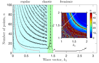
Figure 4: Number of points $n$ generated by the map Eq. (6) depending on the starting wave vector $k_{1}$ for $k_{2}=k_{1}+0.4$. We used 100 iterations for each of the $1.6\times 10^{5}$ starting values of $k_{1}=0.4\ldots\pi-0.4$ (white line in the inset). Only the points below the threshold $|\mathop{\mathrm{missing}}{Im}\nolimits q|<1$ have been included in the map. Inset shows the dependence of $n$ on both starting wave vectors $k_{1}$ and $k_{2}$ varying near the center of the Brillouin zone. The grid step is $8\times 10^{-3}$ and 70 iterations were made for the inset.

When the evanescent waves with complex $q,K$ are taken into account, the maps Eq. (6),(7) can generate infinite ergodic trajectories. In order to build ergodic trajectory we use the fact that the map Eq. (7) provides two values of $\cos\widetilde{K}$ for each value of $\cos K$. By choosing between these two values we can build an infinite trajectory that turns around the points $\cos K=\cos\widetilde{K}=\pm 1$ and never repeats itself, as shown in Fig. 3(e). By construction, this trajectory includes evanescent waves, where $|\cos K|>1$ and the polariton wave vectors $k_{1,2}=K\pm q/2$ are complex. This is also seen in Fig. 3(b), where green points represent complex $k_{1,2}$ that do not lie on the real isoenergy contour. Such trajectories lead to a dense irregular distribution of wave vectors in the Fourier space and explain formation of chaotic states Fig. 2(b,e).

In order to examine the transition from regular to chaotic states in more detail we plot in Fig. 4 the number of points generated by the map Eq. (6) depending on the initial polariton wave vector $k_{1}$ for $k_{2}=k_{1}+0.4$. Three distinct ranges of wave vectors can be identified. In the range $0\leq k_{1}\lesssim 1.3$ the map generates cycles of type Fig. 3(a,d). The points in Fig. 4 group into “lines” that correspond to cycles with different number of loops made around the ellipse in Fig. 3(d). For example, the red curve $n=\sqrt{2}\pi/k_{1}$ shows the approximate number of points for a one-loop cycle. In our calculation we neglected strongly evanescent waves with $|\mathop{\mathrm{missing}}{Im}\nolimits q|>\mathop{\mathrm{missing}}{Im}\nolimits q^{*}=1$ assuming that their contribution to the wave function is exponentially weak. Such cutoff leads to a steep decrease of the number of generated points for $k_{1}\gtrsim 1.5$ (the results are not qualitatively sensitive to the cutoff value). Only a small number of wave vectors are generated, which corresponds to the fermionized states of the type Fig. 3(c,f). Finally, there is a narrow peak in the transition region, centered at around $k_{1}\approx 1.4$, corresponding to the chaotic states of the type Fig. 3(b,e). Inset of Fig. 4 shows the same number of generated points depending on the values of both initial wave vectors $k_{1}$ and $k_{2}$. The calculation also reveals two distinct regions of fermionic and regular states, with a narrow chaotic region in between.

To summarize, we have obtained a nonlinear map describing two-polariton interactions in $k$-space. The number of non-evanescent waves generated by this map is a good predictor whether a given quantum state is regular non-integrable (small values of $k_{1,2}$), chaotic (intermediate values of $k_{1,2}$) or integrable fermionized ($k_{1,2}$ close to the edge of the Brillouin zone). Our findings apply to various two-particle systems and will be hopefully useful also for the many-body setups. Experimental verification could be done with already available arrays of tens of superconducting qubits  Kim et al. (2020); Brehm et al. (2020) with the possibility to excite and probe every qubit separately Ye et al. (2019).

Online Supplementary Materials

Appendix A Derivation of the two-polariton Hamiltonian

In this section we provide some details on the derivation of the two-polariton Schrödinger equation Eq. (1) in the main text. The derivation follows Supplementary Materials of Refs. Ke et al. (2019); Zhong et al. (2020), alternative but equivalent derivations can be found in Refs. Caneva et al. (2015); Zhang et al. (2020).

We start with the Hamiltonian for interaction between array of atoms and photons

$$\mathcal{H}=\sum\limits_{k}\omega_{k}a_{k}^{{\dagger}}a_{k}^{\vphantom{{\dagger}}}+\sum\limits_{j}\omega_{0}b_{j}^{{\dagger}}b_{j}^{\vphantom{{\dagger}}}+\frac{\chi}{2}\sum\limits_{j}b_{j}^{{\dagger}}b_{j}^{{\dagger}}b_{j}^{\vphantom{{\dagger}}}b_{j}^{\vphantom{{\dagger}}}\\ +\frac{g}{\sqrt{L}}\sum\limits_{j,k}(b_{j}^{{\dagger}}a_{k}{\rm e}^{{\rm i}kz_{j}}+b_{j}a_{k}^{{\dagger}}{\rm e}^{-{\rm i}kz_{j}})\>.$$ (S1)

Here, $a_{k}$ are the annihilation operators for the waveguide photons with the wave vectors $k$, frequencies $\omega_{k}=c|k|$ and the velocity $c$, $g$ is the interaction constant, $L$ is the normalization length, and $b_{j}$ are the (bosonic) annihilation operators for the qubit excitations with the frequency $\omega_{0}$, located at the point $z_{j}$. In Eq. (S1), we consider the general case of anharmonic many-level qubits. The two-level case can be obtained in the limit of large anharmonicity ($\chi\to\infty$) where the multiple occupation is suppressed Zheng and Baranger (2013); Poshakinskiy and Poddubny (2016); Abrikosov (1965). The photonic degrees of freedom can be integrated out in Eq. (S1) yielding the effective Hamiltonian Caneva et al. (2015); Ivchenko (2005)

$$H_{mn}=\omega_{0}\delta_{nm}-{\rm i}\Gamma_{0}{\rm e}^{{\rm i}\omega|z_{m}-z_{n}|/c}$$ (S2)

describing the motion of qubit excitations

$$H_{mn} = \omega_{0}\delta_{m,n}+g^{2}\sum_{l,l^{\prime}}\int\frac{{\rm d}k}{2\pi}{\rm e}^{{\rm i}(z_{l}-z_{l}^{\prime})}\frac{\langle 0|b_{m}a_{k}b_{l}^{\dagger}b_{l}^{\prime}a_{k}^{{\dagger}}b_{n}^{\dagger}|0\rangle}{\omega-\omega_{k}+{0^{+}}{\rm i}}$$ (S3)

$$= \omega_{0}\delta_{m,n}+g^{2}\sum_{l,l^{\prime}}\int\frac{{\rm d}k}{2\pi}\frac{{\rm e}^{{\rm i}(z_{m}-z_{n})}}{\omega-c|k|+{0^{+}}{\rm i}}$$

$$= \omega_{0}\delta_{m,n}-{\rm i}\frac{g^{2}}{c}{\rm e}^{{\rm i}\omega|z_{m}-z_{n}|/c}\>.$$

Here we have introduced the radiative decay rate $\Gamma_{0}={g^{2}}/{c}$ and implied the rotating wave approximation. From now on we will count the energy from $\omega_{0}$ and hence omit the $\omega_{0}\delta_{m,n}$ term. Then, the total effective Hamiltonian is given as

$$\mathcal{H}=\sum\limits_{m,n=1}^{N}H_{m,n}(\omega_{0})b_{m}^{{\dagger}}b_{n}+\frac{\chi}{2}\sum\limits_{m=1}^{N}b_{m}^{{\dagger}}b_{m}^{{\dagger}}b_{m}^{\vphantom{{\dagger}}}b_{m}^{\vphantom{{\dagger}}}\>.$$ (S4)

Here we use the Markovian approximation, by replacing the phase $\omega|z_{m}-z_{n}|/c$ in Eq. (S3) by $\omega_{0}|z_{m}-z_{n}|/c$. When being limited to the subspace with only two excitations, we can construct the effective two-photon Hamiltonian

$$H^{(2)}_{i_{1}i_{2};j_{1}j_{2}}=\delta_{i_{2},j_{2}}H^{(1)}_{i_{1}j_{1}}+\delta_{i_{1},j_{1}}H^{(1)}_{i_{2}j_{2}}+U_{i_{1}i_{2};j_{1}j_{2}}$$ (S5)

where $i_{1},i_{2},j_{1},j_{2}=1\ldots N$ and

$$\mathcal{U}_{i_{1}i_{2};j_{1}j_{2}}=\delta_{i_{1}i_{2}}\delta_{j_{1}j_{2}}\delta_{i_{1}j_{1}}\chi\>.$$ (S6)

The linear eigenvalue problem to obtain the two-particle excitations then reads

$$H_{mn^{\prime}}\psi_{n^{\prime}n}+\psi_{mn^{\prime}}H_{n^{\prime}n}+\chi\delta_{mn}\psi_{nn}=2\varepsilon\psi_{mn}$$ (S7)

We now proceed to the limit of two-level atoms, when $\chi\to\infty$. Importantly, even though $\psi_{nn}\to 0$ for $\chi\to\infty$, we still have $\chi\psi_{nn}\to\rm const$. The value of $\chi\psi_{nn}$ for large $\chi$ can be calculated perturbatively

$$\chi\psi_{nn}=-\sum\limits_{n^{\prime}\neq n}(H_{nn^{\prime}}\psi_{n^{\prime}n}+\psi_{nn^{\prime}}H_{n^{\prime}n})=\\ -2\sum\limits_{n^{\prime}\neq n}H_{nn^{\prime}}\psi_{n^{\prime}n}=-2\sum\limits_{n^{\prime}=1}^{N}H_{nn^{\prime}}\psi_{n^{\prime}n}\>.$$ (S8)

Hence, we can rewrite the Schrödinger equation in the limit $\chi\to\infty$ as

$$H_{mn^{\prime}}\psi_{n^{\prime}n}+\psi_{mn^{\prime}}H_{n^{\prime}n}-2\delta_{mn}H_{nn^{\prime}}\psi_{n^{\prime}n}=2\varepsilon\psi_{mn}$$ (S9)

in agreement with Eq. (1) in the main text.

Appendix B Dispersion equation

Here we provide the details of the derivation of the dispersion equation for the relative motion of two interacting polaritons in the center of mass reference frame. We start from the Schrödinger equation Eq. (1) in the main text, that reads Ke et al. (2019)

$$(H^{-1}\Psi+\Psi H^{-1})_{nm}- 2\delta_{nm}(\Psi H^{-1})_{nn}$$

$$=2\varepsilon(H^{-1}\Psi H^{-1})_{nm}\>.$$ (S10)

The inverse of the matrix $H_{mn}=-{\rm i}\Gamma_{0}{\rm e}^{{\rm i}\varphi|m-n|}$ is a tri-diagonal matrix Poddubny (2020) that explicitly reads

$$[H^{-1}]_{rs}=\frac{1}{\Gamma_{0}}\begin{pmatrix}-\frac{1}{2}\cot{\varphi}+\frac{{\rm i}}{2}&\frac{1}{2\sin{\varphi}}&0&\ldots\\ \frac{1}{2\sin{\varphi}}&-\cot{\varphi}&\frac{1}{2\sin{\varphi}}&\ldots\\ &&\ddots&\\ \ldots&\frac{1}{2\sin{\varphi}}&-\cot{\varphi}&\frac{1}{2\sin{\varphi}}\\ \ldots&0&\frac{1}{2\sin{\varphi}}&-\frac{1}{2}\cot{\varphi}+\frac{{\rm i}}{2}\end{pmatrix}\>.$$ (S11)

Due to the translation symmetry of the infinite array the two-polariton wavefunction can be sought in the form

$$\Psi_{mn}={\rm e}^{{\rm i}K(m+n)}\psi_{r},\quad r=|m-n|$$ (S12)

where $K$ is the center of mass wave vector and $\psi_{r}=\psi_{-r}$ due to bosonic symmetry. Substituting Eq. (S12) into the Schrödinger equation (B) we obtain the equations the wavefunction $\psi_{r}$ that describes relative motion of the two interacting polaritons. The advantage of the equation Eq. (B) based on the inverse Hamiltonian matrix over the center-of-mass motion equation in Supplementary Materials of Zhang and Mølmer (2019) is that it includes only nearest-neighbor couplings. Hence, for $r=|n-m|\geq 2$ we obtain a conceptually simple tight-binding equation

$$\frac{\cos K}{\sin{\varphi}}(\psi_{r-1}+\psi_{r+1})-2\cot{\varphi}\psi_{r}\\ =\frac{\varepsilon}{2\Gamma_{0}\sin^{2}{\varphi}}[(4\cos^{2}{\varphi}+2\cos 2K)\psi_{r}\\ +\psi_{r-2}+\psi_{r+2}-4\cos\varphi\cos K(\psi_{r-1}+\psi_{r+1})]\>.$$ (S13)

The values of the relative distance $r=0$ and $r=1$ are special because one should take into account include non-zero contributions from the polariton-polariton interaction term $2\delta_{nm}(\Psi H^{-1})_{nn}$ in Eq. (B). Specifically, for $r=0$ we find

$$\left(2\cos^{2}{\varphi}+\cos 2K\right)\psi_{{0}}-4\,\cos{\varphi}\cos K\psi_{{1}}+\psi_{2}=0\>.$$ (S14)

and for $r=1$ the Schrödinger equation reads

$$\frac{\cos K}{\sin{\varphi}}(\psi_{0}+\psi_{2})-2\cot{\varphi}\psi_{1}\\ =\frac{\varepsilon}{2\Gamma_{0}\sin^{2}{\varphi}}[(4\cos^{2}{\varphi}+2\cos 2K+1)\psi_{1}\\ +\psi_{3}-4\cos\varphi\cos K(\psi_{0}+\psi_{2})]\>.$$ (S15)

For $r\geq 2$ we can use the following ansatz in Eq. (S13)

$$\psi_{r}={\rm e}^{{\rm i}qr/2}$$ (S16)

which leads to

$$2\varepsilon=\frac{\Gamma_{0}\cos{\varphi}}{\cos k_{1}-\cos{\varphi}}+\frac{2\Gamma_{0}\cos{\varphi}}{\cos k_{2}-\cos{\varphi}}$$ (S17)

where $k_{1,2}=K\pm q/2$, which is Eq. (2) in the main text. This is the presentation of the total pair energy $2\varepsilon$ is given by a sum of energies of non-interacting polaritons with the wave vectors $k_{1}$ and $k_{2}$. It is more convenient to rewrite the dispersion equation Eq. (S17) as

$$-\varepsilon\,({z}^{4}+1)+2\left(2\cos{\varphi}\varepsilon+\sin{\varphi}\right)\cos K({z}^{3}+z)\\ -2\left(2\cos^{2}{\varphi}\varepsilon+\varepsilon\cos 2K+\sin 2{\varphi}\right){z}^{2}=0\>,$$ (S18)

where $z={\rm e}^{{\rm i}q/2}$. The representation Eq. (S18) explicitly shows that there are four inequivalent solutions $z_{1},1/z_{1},z_{2},1/z_{2}$ for each value of total energy of two polaritons $2\varepsilon$ and center of mass wave vector $K$. Dividing Eq. (S18) by $z^{2}$ and using the relation $z+1/z=2\cos\frac{q}{2}$ we find for $\varphi\ll 1$

$$\left(\cos K-\cos\frac{q}{2}\right)^{2}-\frac{\varphi\Gamma_{0}}{\varepsilon}(\cos K\cos\frac{q}{2}-1)=0\>.$$ (S19)

which is equivalent to the map Eq. (7) in the main text.

Explicit expressions for the wave vectors $q$ can be most easily obtained for $\varphi\ll 1$ when $\omega(k)\approx-2\varphi/k^{2}$ and Eq. (S17) simplifies to

$$\varepsilon=-\frac{\Gamma_{0}{\varphi}}{k_{1}^{2}}-\frac{\Gamma_{0}{\varphi}}{k_{2}^{2}}\>.$$ (S20)

Solution of this equation for $q$ vs $K$ yields

$$q_{1,\pm}^{2} =\pm\sqrt{K^{2}-\frac{4}{w}-\frac{4\sqrt{1-K^{2}w}}{w}},$$ (S21)

$$q_{2,\pm}^{2} =\pm\sqrt{K^{2}-\frac{4}{w}+\frac{4\sqrt{1-K^{2}w}}{w}},$$ (S22)

where $\varepsilon=w{\varphi}\Gamma_{0}$.

Appendix C Bethe ansatz

In this section we provide more details on the construction of Bethe ansatz in the infinite array. The idea behind this construction is to present the two-polariton wavefunction as a superposition of single-polariton states and then to satisfy Eqs. (S14),(S15) describing polariton-polariton interactions. We start with a general Bethe ansatz expansion

$$\psi_{m}(K,\varepsilon)=\sum\limits_{\nu=1}^{4}{\rm e}^{{\rm i}q_{\nu}m/2}A_{\nu}$$ (S23)

that presents the two-polariton wavefunction as a superposition of solutions with given center-of-mass wave vector $K$ and four possible values of relative motion wave vectors $q$. Substituting Eq. (S23) in Eq. (S14) we find

$$\sum\limits_{\nu=1}^{4}A_{\nu}\bigl{[}\left(2\cos^{2}{\varphi}+\cos 2K\right)\\ -4\,\cos{\varphi}\cos K{\rm e}^{{\rm i}q_{\nu}/2}+{\rm e}^{{\rm i}q_{\nu}}\bigr{]}=0\>.$$ (S24)

The same procedure for Eq. (S15)

$$\sum\limits_{\nu=1}^{4}A_{\nu}\sin\tfrac{q_{\nu}}{2}=0\>.$$ (S25)

Solution of Eqs. (S24),(S25) allows us to express two of the $A$ coefficients vs other two ones. Taking into account that the four wave vectors $q_{\nu}$ come into two pairs $q_{A},-q_{A}$ and $q_{B},-q_{B}$ , we can rewrite Eq. (S23) as

$$\psi_{m}(K,\varepsilon)=(A{\rm e}^{{\rm i}q_{A}m/2}+\widetilde{A}{\rm e}^{-{\rm i}q_{A}m/2})\\ +(B{\rm e}^{{\rm i}q_{B}m/2}+\widetilde{B}{\rm e}^{-{\rm i}q_{B}m/2})$$ (S26)

and find

$$\widetilde{A}= \frac{\sin\frac{q_{A}}{2}f^{*}(q_{B})+\sin\frac{q_{B}}{2}f(q_{A})}{\sin\frac{q_{A}}{2}f^{*}(q_{B})\sin\frac{q_{B}}{2}f^{*}(q_{A})}A$$ (S27)

$$+ \sin\frac{q_{B}}{2}\frac{f^{*}(q_{B})+f(q_{B})}{\sin\frac{q_{A}}{2}f^{*}(q_{B})-\sin\frac{q_{B}}{2}f^{*}(q_{A})}B\>,$$

$$\widetilde{B}= -\frac{\sin\frac{q_{A}}{2}f(q_{B})+\sin\frac{q_{B}}{2}f(q_{A})^{*}}{\sin\frac{q_{A}}{2}f^{*}(q_{B})-\sin\frac{q_{B}}{2}f^{*}(q_{A})}B$$ (S28)

$$- \sin\frac{q_{A}}{2}\frac{f^{*}(q_{A})+f(q_{A})}{\sin\frac{q_{A}}{2}f^{*}(q_{B})-\sin\frac{q_{B}}{2}f^{*}(q_{A})}A\>,$$

where

$$f(q)=\left(2\cos^{2}{\varphi}+\cos 2K\right)-4\,\cos{\varphi}\cos K{\rm e}^{{\rm i}q/2}+{\rm e}^{{\rm i}q}\>.$$ (S29)

References

- Roy et al. (2017) D. Roy, C. M. Wilson, and O. Firstenberg, “Colloquium: strongly interacting photons in one-dimensional continuum,” Rev. Mod. Phys. 89, 021001 (2017).
- Chang et al. (2018) D. E. Chang, J. S. Douglas, A. González-Tudela, C.-L. Hung, and H. J. Kimble, “Colloquium: quantum matter built from nanoscopic lattices of atoms and photons,” Rev. Mod. Phys. 90, 031002 (2018).
- van Loo et al. (2013) A. F. van Loo, A. Fedorov, K. Lalumiere, B. C. Sanders, A. Blais, and A. Wallraff, “Photon-mediated interactions between distant artificial atoms,” Science 342, 1494–1496 (2013).
- Corzo et al. (2019) N. V. Corzo, J. Raskop, A. Chandra, A. S. Sheremet, B. Gouraud, and J. Laurat, “Waveguide-coupled single collective excitation of atomic arrays,” Nature 566, 359–362 (2019).
- Mirhosseini et al. (2019) M. Mirhosseini, E. Kim, X. Zhang, A. Sipahigil, P. B. Dieterle, A. J. Keller, A. Asenjo-Garcia, D. E. Chang, and O. Painter, “Cavity quantum electrodynamics with atom-like mirrors,” Nature 569, 692–697 (2019).
- Brehm et al. (2020) J. D. Brehm, A. N. Poddubny, A. Stehli, T. Wolz, H. Rotzinger, and A. V. Ustinov, “Waveguide bandgap engineering with an array of superconducting qubits,” (2020), arXiv:2006.03330 [quant-ph] .
- Prasad et al. (2020) A. S. Prasad, J. Hinney, S. Mahmoodian, K. Hammerer, S. Rind, P. Schneeweiss, A. S. Sørensen, J. Volz, and A. Rauschenbeutel, “Correlating photons using the collective nonlinear response of atoms weakly coupled to an optical mode,” Nature Photonics (2020), 10.1038/s41566-020-0692-z.
- Leung and Sanders (2012) P. M. Leung and B. C. Sanders, “Coherent control of microwave pulse storage in superconducting circuits,” Phys. Rev. Lett. 109, 253603 (2012).
- Zheng et al. (2013) H. Zheng, D. Gauthier, and H. Baranger, “Waveguide-QED-based photonic quantum computation,” Phys. Rev. Lett. 111, 090502 (2013).
- Zheng and Baranger (2013) H. Zheng and H. U. Baranger, “Persistent quantum beats and long-distance entanglement from waveguide-mediated interactions,” Phys. Rev. Lett. 110, 113601 (2013).
- Johnson et al. (2019) A. Johnson, M. Blaha, A. E. Ulanov, A. Rauschenbeutel, P. Schneeweiss, and J. Volz, “Observation of collective superstrong coupling of cold atoms to a 30-m long optical resonator,” Phys. Rev. Lett. 123, 243602 (2019).
- Kimble (2008) H. J. Kimble, “The quantum internet,” Nature 453, 1023 (2008).
- Noh and Angelakis (2016) C. Noh and D. G. Angelakis, “Quantum simulations and many-body physics with light,” Reports on Progress in Physics 80, 016401 (2016).
- Xu et al. (2018) K. Xu, J.-J. Chen, Y. Zeng, Y.-R. Zhang, C. Song, W. Liu, Q. Guo, P. Zhang, D. Xu, H. Deng, K. Huang, H. Wang, X. Zhu, D. Zheng, and H. Fan, “Emulating many-body localization with a superconducting quantum processor,” Phys. Rev. Lett. 120, 050507 (2018).
- Iorsh et al. (2020) I. Iorsh, A. Poshakinskiy, and A. Poddubny, “Waveguide quantum optomechanics: Parity-time phase transitions in ultrastrong coupling regime,” Phys. Rev. Lett. 125, 183601 (2020).
- Faddeev (2013) L. D. Faddeev, “The new life of complete integrability,” Physics-Uspekhi 56, 465–472 (2013).
- Moore (2017) J. E. Moore, “A perspective on quantum integrability in many-body-localized and Yang–Baxter systems,” Phil. Trans. Roy. Soc. A 375, 20160429 (2017).
- Bunakov (2016) V. E. Bunakov, “Quantum signatures of chaos or quantum chaos?” Physics of Atomic Nuclei 79, 995–1009 (2016).
- Ullmo (2008) D. Ullmo, “Many-body physics and quantum chaos,” Reports on Progress in Physics 71, 026001 (2008).
- D’Alessio et al. (2016) L. D’Alessio, Y. Kafri, A. Polkovnikov, and M. Rigol, “From quantum chaos and eigenstate thermalization to statistical mechanics and thermodynamics,” Advances in Physics 65, 239–362 (2016).
- Aßmann et al. (2016) M. Aßmann, J. Thewes, D. Fröhlich, and M. Bayer, “Quantum chaos and breaking of all anti-unitary symmetries in Rydberg excitons,” Nature Materials 15, 741–745 (2016).
- Maldacena et al. (2016) J. Maldacena, S. H. Shenker, and D. Stanford, “A bound on chaos,” J. High Energy Phys. 2016, 106 (2016).
- Morita (2019) T. Morita, “Thermal emission from semiclassical dynamical systems,” Phys. Rev. Lett. 122, 101603 (2019).
- Birnbaum et al. (2005) K. M. Birnbaum, A. Boca, R. Miller, A. D. Boozer, T. E. Northup, and H. J. Kimble, “Photon blockade in an optical cavity with one trapped atom,” Nature (London) 436, 87–90 (2005).
- Lieb and Liniger (1963) E. H. Lieb and W. Liniger, “Exact analysis of an interacting Bose gas. I. The general solution and the ground state,” Phys. Rev. 130, 1605–1616 (1963).
- McGuire (1964) J. B. McGuire, “Study of exactly soluble one-dimensional n-body problems,” J. Math. Phys. 5, 622–636 (1964).
- Gaudin (1971) M. Gaudin, “Boundary energy of a Bose gas in one dimension,” Phys. Rev. A 4, 386–394 (1971).
- Beims et al. (2007) M. W. Beims, C. Manchein, and J. M. Rost, “Origin of chaos in soft interactions and signatures of nonergodicity,” Phys. Rev. E 76, 056203 (2007).
- Shepelyansky (2016) D. L. Shepelyansky, “Chaotic delocalization of two interacting particles in the classical Harper model,” The European Physical Journal B 89, 157 (2016).
- Van Vessen et al. (2001) M. Van Vessen, M. C. Santos, B. K. Cheng, and M. G. E. da Luz, “Origin of quantum chaos for two particles interacting by short-range potentials,” Phys. Rev. E 64, 026201 (2001).
- Casati and Prosen (1999) G. Casati and T. Prosen, “Mixing property of triangular billiards,” Phys. Rev. Lett. 83, 4729–4732 (1999).
- Zhang and Mølmer (2019) Y.-X. Zhang and K. Mølmer, “Theory of subradiant states of a one-dimensional two-level atom chain,” Phys. Rev. Lett. 122, 203605 (2019).
- Zhong et al. (2020) J. Zhong, N. A. Olekhno, Y. Ke, A. V. Poshakinskiy, C. Lee, Y. S. Kivshar, and A. N. Poddubny, “Photon-mediated localization in two-level qubit arrays,” Phys. Rev. Lett. 124, 093604 (2020).
- Poshakinskiy et al. (2020) A. V. Poshakinskiy, J. Zhong, Y. Ke, N. A. Olekhno, C. Lee, Y. S. Kivshar, and A. N. Poddubny, “Quantum Hall phase emerging in an array of atoms interacting with photons,” (2020), arXiv:2003.08257 [quant-ph] .
- Ivchenko (1991) E. L. Ivchenko, “Excitonic polaritons in periodic quantum-well structures,” Sov. Phys. Sol. State 33, 1344–1346 (1991).
- Albrecht et al. (2019) A. Albrecht, L. Henriet, A. Asenjo-Garcia, P. B. Dieterle, O. Painter, and D. E. Chang, “Subradiant states of quantum bits coupled to a one-dimensional waveguide,” New J. Phys. 21, 025003 (2019).
- Caneva et al. (2015) T. Caneva, M. T. Manzoni, T. Shi, J. S. Douglas, J. I. Cirac, and D. E. Chang, “Quantum dynamics of propagating photons with strong interactions: a generalized input–output formalism,” New Journal of Physics 17, 113001 (2015).
- Ke et al. (2019) Y. Ke, A. V. Poshakinskiy, C. Lee, Y. S. Kivshar, and A. N. Poddubny, “Inelastic scattering of photon pairs in qubit arrays with subradiant states,” Phys. Rev. Lett. 123, 253601 (2019).
- Berry (1977) M. V. Berry, “Regular and irregular semiclassical wavefunctions,” Journal of Physics A: Mathematical and General 10, 2083–2091 (1977).
- Poddubny (2020) A. N. Poddubny, “Quasiflat band enabling subradiant two-photon bound states,” Phys. Rev. A 101, 043845 (2020).
- Batchelor (2007) M. T. Batchelor, “The Bethe ansatz after 75 years,” Physics Today 60, 36–40 (2007).
- Zhang et al. (2012) J. M. Zhang, D. Braak, and M. Kollar, “Bound states in the continuum realized in the one-dimensional two-particle Hubbard model with an impurity,” Phys. Rev. Lett. 109, 116405 (2012).
- Longhi and Della Valle (2013) S. Longhi and G. Della Valle, “Tamm–Hubbard surface states in the continuum,” J. Phys: Cond. Matter 25, 235601 (2013).
- Kim et al. (2020) E. Kim, X. Zhang, V. S. Ferreira, J. Banker, J. K. Iverson, A. Sipahigil, M. Bello, A. Gonzalez-Tudela, M. Mirhosseini, and O. Painter, “Quantum electrodynamics in a topological waveguide,” (2020), arXiv:2005.03802 [quant-ph] .
- Ye et al. (2019) Y. Ye, Z.-Y. Ge, Y. Wu, S. Wang, M. Gong, Y.-R. Zhang, Q. Zhu, R. Yang, S. Li, F. Liang, J. Lin, Y. Xu, C. Guo, L. Sun, C. Cheng, N. Ma, Z. Y. Meng, H. Deng, H. Rong, C.-Y. Lu, C.-Z. Peng, H. Fan, X. Zhu, and J.-W. Pan, “Propagation and localization of collective excitations on a 24-qubit superconducting processor,” Phys. Rev. Lett. 123, 050502 (2019).
- Zhang et al. (2020) Y.-X. Zhang, C. Yu, and K. Mølmer, “Subradiant bound dimer excited states of emitter chains coupled to a one dimensional waveguide,” Phys. Rev. Research 2, 013173 (2020).
- Poshakinskiy and Poddubny (2016) A. V. Poshakinskiy and A. N. Poddubny, “Biexciton-mediated superradiant photon blockade,” Phys. Rev. A 93, 033856 (2016).
- Abrikosov (1965) A. Abrikosov, “Electron scattering on magnetic impurities in metals and anomalous resistivity effects,” Physics Physique Fizika 2, 5 (1965).
- Ivchenko (2005) E. L. Ivchenko, Optical Spectroscopy of Semiconductor Nanostructures (Alpha Science International, Harrow, UK, 2005).