BeyondPlanck XV. Polarized foreground emission
between 30 and 70 GHz

We constrain polarized foreground emission between 30 and 70 GHz with the Planck Low Frequency Instrument (LFI) and WMAP data within the global Bayesian BeyondPlanck framework. We combine for the first time full-resolution Planck LFI time-ordered data with low-resolution WMAP sky maps at 33, 40 and 61 GHz. Spectral parameters are fit with a likelihood defined at the native resolution of each frequency channel. This analysis represents the first implementation of true multi-resolution component separation applied to CMB observations for both amplitude and spectral energy distribution (SED) parameters. For synchrotron emission, we approximate the SED as a power-law in frequency and find that the low signal-to-noise ratio of the current data strongly limits the number of free parameters that may be robustly constrained. We partition the sky into four large disjoint regions (High Latitude; Galactic Spur; Galactic Plane; and Galactic Center), each associated with its own power-law index. We find that the High Latitude region is prior-dominated, while the Galactic Center region is contaminated by residual instrumental systematics. The two remaining regions appear to be signal-dominated, and for these we derive spectral indices of $\beta_{\mathrm{s}}^{\mathrm{Spur}}=-3.17\pm 0.06$ and $\beta_{\mathrm{s}}^{\mathrm{Plane}}=-3.03\pm 0.07$, in good agreement with previous results. For thermal dust emission we assume a modified blackbody model and we fit a single power-law index across the full sky. We find $\beta_{\mathrm{d}}=1.64\pm 0.03$, which is slightly steeper than reported from Planck HFI data, but still statistically consistent at the 2 $\sigma$ confidence level.

1 Introduction

One of the most important sources of information about the early universe is the cosmic microwave background (CMB; Penzias & Wilson 1965). By mapping and characterizing the statistical properties of this signal, cosmologists have during the last few decades constrained both the composition and evolution of the universe to percent accuracy (e.g., Bennett et al. 2013; Planck Collaboration I 2020).

As shown by the COBE-FIRAS experiment (Mather et al. 1994), the frequency spectrum of the CMB may to a very high precision be described in terms of a blackbody with a mean temperature of $T_{\mathrm{CMB}}=2.7255\thinspace\mathrm{K}$ (Fixsen 2009). As such, its peak intensity occurs at $161\thinspace\mathrm{GHz}$, and the primary frequency range considered by most CMB experiments is therefore around 30 to 300 GHz. In addition to the CMB, a diverse range of astrophysical emission mechanisms contribute to the observed signal at these frequencies, both of Galactic and extragalactic origin. For intensity, the main contributors are synchrotron, free-free, CO, thermal dust, and anomalous microwave emission, while for polarization, synchrotron and thermal dust emission dominate (e.g., Bennett et al. 2013; Planck Collaboration IV 2018, and references therein).

At the foreground minimum, around 80 GHz, the CMB anisotropies dominate over the combined foreground amplitude over most of the sky (Planck Collaboration Int. XLVI 2016), and CMB temperature extraction is therefore relatively straightforward. The same does not hold true for polarization, even at the foreground minimum, the sum of synchrotron and thermal dust emission is greater than the polarized CMB by almost a full order of magnitude on large angular scales. Polarized foreground estimation therefore plays a critically important role in contemporary cosmology, as such observations may contain signatures of primordial gravitational waves created during the Big Bang (e.g., Kamionkowski & Kovetz 2016, and references therein), and thereby provide a unique observational window on inflation and physics at the Planck energy scale.

However, the amplitude of the primordial gravitational wave signal is expected to be smaller than 10–100 nK on large angular scales (Tristram et al. 2021). This, combined with a plethora of confounding instrumental effects, such as temperature-to-polarization leakage (Paradiso et al. 2022), correlated noise (Ihle et al. 2022) and calibration uncertainties (Gjerløw et al. 2022), makes high-precision CMB polarization science a particularly difficult challenge. Furthermore, as summarized by the Planck team in a document called “Lessons learned from Planck”, the quality of current state-of-the-art CMB observations is limited by the interplay between instrumental and foreground effects. This insight formed the basis for the BeyondPlanck project (BeyondPlanck 2022), which aims to implement an end-to-end Bayesian CMB analysis framework that jointly accounts for both systematic effects and astrophysical foregrounds, starting from raw time-ordered data. This framework employs an explicit parametric model that accounts jointly for cosmological, astrophysical, and instrumental parameters. These parameters are sampled with Markov Chain Monte Carlo methods, such as Gibbs sampling, as implemented in the Commander software. (Eriksen et al. 2004, 2008; Galloway et al. 2022).

The BeyondPlanck results are described in a suite of 17 companion papers (see BeyondPlanck 2022, and references therein), each focusing on a particular aspect of the analysis. The current paper focuses on polarized foreground characterization, both in terms of algorithms and results, with special attention paid to the spectral properties of polarized synchrotron emission on large angular scales. The current BeyondPlanck analysis considers only the Planck LFI observations in terms of time-ordered data, although selected preprocessed external data sets are also included to break critical degeneracies, specifically WMAP measurements between 33 and 61 GHz (Bennett et al. 2013), Planck HFI measurements at 353 and 857 GHz (Planck Collaboration I 2020; Planck Collaboration Int. LVII 2020), and the Haslam 408 MHz measurements (Haslam et al. 1982), the latter two are only included in temperature. Overall, the main emphasis of the present analysis lies on frequencies below the foreground minimum, between 30 and 70 GHz, and in particular on the spectral behavior of polarized synchrotron and thermal dust emission within this critically important frequency range. The present analysis is the first to combine high-resolution Planck measurements with low-resolution WMAP observations into a single coherent model, when estimating both foreground amplitudes and spectral parameters.

The rest of this paper is structured as follows: In Sect. 2, we briefly review the BeyondPlanck data model, focusing on the aspects that are relevant for polarized foreground analysis. In Sect. 3, we review the data sets that are included in the current analysis. In Sect. 4 we describe the basic algorithms, and connect these to the larger Gibbs sampling framework outlined in BeyondPlanck (2022). Results are presented in Sect. 5, before we conclude in Sect. 6.

2 The BeyondPlanck data model

As described by BeyondPlanck (2022), the main goal of this project is to perform end-to-end Bayesian CMB analysis, building on well-established statistical methods. The first step in any such Bayesian analysis is to write down an explicit parametric data model that will be fit to observations through posterior mapping techniques. For BeyondPlanck, we adopt the following model for this purpose,

$$\begin{split}d_{j,t}=g_{j,t}&\@tens{P}_{tp,j}\left[\@tens{B}^{\mathrm{symm}}_{pp^{\prime},j}\sum_{c}\@tens{M}_{cj}(\beta_{p^{\prime}},\Delta_{\mathrm{bp}}^{j})a^{c}_{p^{\prime}}+\@tens{B}^{\mathrm{asymm}}_{j}\left(s^{\mathrm{orb}}_{j}+s^{\mathrm{fsl}}_{j}\right)\right]+\\ +&s^{\mathrm{1hz}}_{j,t}+n^{\mathrm{corr}}_{j,t}+n^{\mathrm{w}}_{j,t},\end{split}$$ (1)

where $j$ represents a radiometer (or detector) label, $t$ indicates a single time sample, $p$ denotes a single pixel on the sky, and $c$ represents one single astrophysical signal component. Further, $d_{j,t}$ denotes the measured time-ordered data; $g_{j,t}$ denotes the instrumental gain; $\@tens{P}_{tp,j}$ is a pointing matrix; $\@tens{B}_{pp^{\prime},j}$ denotes beam convolution; $\@tens{M}_{cj}(\beta_{p},\Delta_{\mathrm{bp}})$ denotes a foreground mixing matrix that depends on some set of spectral parameters, $\beta$, and instrumental bandpass specification, $\Delta_{\mathrm{bp}}$; $a^{c}_{p}$ is the amplitude of astrophysical component $c$ in pixel $p$, measured at the same reference frequency as the mixing matrix $\@tens{M}$, and expressed in brightness temperature units; $s^{\mathrm{orb}}_{j,t}$ is the orbital CMB dipole signal; $s^{\mathrm{fsl}}_{j,t}$ denotes the contribution from far side-lobes; $s^{\mathrm{1hz}}_{j,t}$ denotes the contribution from electronic 1 Hz spikes; $n^{\mathrm{corr}}_{j,t}$ denotes correlated instrumental noise; and $n^{\mathrm{w}}_{j,t}$ is uncorrelated instrumental noise with (diagonal) time-domain covariance matrix $\@tens{N}^{\mathrm{w}}_{j}$. For further details regarding any of these objects, we refer the interested reader to BeyondPlanck (2022) and references therein.

The current paper focuses primarily on diffuse astrophysical foregrounds, which for practical purposes are stationary in time, and we are therefore not interested in the time-domain aspects of the model. For this reason, we rewrite Eq. (1) into the following compact form,

$$m_{\nu,p}=\left[\@tens{B}^{\mathrm{symm}}_{pp^{\prime}}\sum_{c}\@tens{M}_{c}(\beta_{p^{\prime}},\Delta_{\mathrm{bp}})a^{c}_{p^{\prime}}\right]+n^{\mathrm{w}}_{p},$$ (2)

where $m_{\nu,p}$ is a binned sky map derived by co-adding all radiometer data within a single frequency channel, and we are for the moment conditioning on all time-domain parameters,

$$\left(\sum_{j\in\nu}\@tens{P}_{j}^{t}(\@tens{N}^{\mathrm{w}}_{j})^{-1}\@tens{P}_{j}\right)\@vec{m}_{\nu}=\sum_{j}\@tens{P}_{j}^{t}(\@tens{N}^{\mathrm{w}}_{j})^{-1}\@vec{r}_{j}.$$ (3)

Here, $\@vec{r}_{j}$ represents the cleaned and calibrated time-ordered data for detector $j$, as defined by Eq. (76) in BeyondPlanck (2022), and full marginalization over time-domain parameters is done iteratively through Gibbs sampling; see Sect. 4.1 for further details.

In this paper, we are particularly interested in the total sky signal, which may be written as follows,

$$\@vec{s}=\@tens{M}\@vec{a}\equiv\sum_{c=1}^{N_{\mathrm{comp}}}\@vec{a}_{c}\thinspace\left[\thinspace U\int f_{c}(\nu;\beta)\thinspace\tau(\nu)\thinspace\mathrm{d}\nu\right].$$ (4)

Here, each astrophysical signal component, $c$, is associated with an overall amplitude parameter $\@vec{a}$; a unit conversion factor $U$ for going from either thermodynamic or intensity units to brightness temperature; a spectral energy density, $f_{c}$, describing the intensity of the component relative to some reference frequency, $\nu_{\mathrm{0}}$; and some set of spectral parameters, $\beta$, which characterize the frequency dependence of the various emission mechanisms. Finally, $\tau$ represents an instrumental bandpass response function that describes the detector sensitivity as a function of frequency. Again, we refer the interested reader to BeyondPlanck (2022) for further details.

2.1 Polarized sky model

We assume in this paper that the polarized microwave sky may be well approximated by three physically distinct components; synchrotron emission, thermal dust emission, and CMB. A spinning dust, or anomalous microwave emission (AME) component is also commonly included in similar studies, however with an upper limit of its polarization fraction at $<$$1\thinspace\%$ (Génova-Santos et al. 2017; Macellari et al. 2011; Herman et al. 2022), we neglect it in this study.

Each component exhibits a distinctly different behavior both in terms of spatial structure and frequency dependence, and must be described by some unique set of spectral parameters, $\beta$. The choice of spectral parameters is both important and nontrivial. On the one hand, it is important that the adopted parametric model for each component is able to provide an acceptable goodness-of-fit, typically as measured by some $\chi^{2}$ statistic. On the other hand, it is also important that the model is not too flexible, as degeneracies between components may increase the effective noise level to arbitrary high levels. Generally speaking, degeneracies also tend to exacerbate instrumental systematic errors, by attempting to accommodate small signal discrepancies within the unconstrained parameters in the signal model. Choosing an appropriate parametric model is thus a delicate trade-off between allowing sufficient flexibility to model the real sky, while not introducing too many parameters, which otherwise may increase both systematic and statistical uncertainties to untenable levels.

For BeyondPlanck, we adopt the following parametric model for the polarized microwave sky,

$$\@vec{s}_{\mathrm{RJ}}= \thinspace\@vec{a}_{\mathrm{CMB}}\thinspace\frac{x^{2}e^{x}}{\left(e^{x}-1\right)^{2}}\frac{\left(e^{x_{0}}-1\right)^{2}}{x_{0}^{2}e^{x_{0}}}\thinspace$$ (5)

$$+ \thinspace\@vec{a}_{\mathrm{s}}\thinspace\left(\frac{\nu}{\nu_{0,\mathrm{s}}}\right)^{\beta_{\mathrm{s}}}\thinspace$$ (6)

$$+ \thinspace\@vec{a}_{\mathrm{d}}\thinspace\left(\frac{\nu}{\nu_{0,\mathrm{d}}}\right)^{\beta_{\mathrm{d}}+1}\frac{e^{h\nu_{\mathrm{0,\mathrm{d}}}/kT_{\mathrm{d}}}-1}{e^{h\nu/kT_{\mathrm{d}}}-1},$$ (7)

where all vectors are expressed in brightness (Rayleigh-Jeans) temperature units; $x=h\nu/kT_{0}$ (where $h$ and $k$ are Planck’s and Boltzmann’s constants respectively and $T_{0}$ is the CMB monopole of 2.7255 K; Fixsen 2009); and $\nu_{0,c}$ is the reference frequency for component $c$, $\@vec{a}$ is its amplitude, $\beta_{\mathrm{s}}$ is the synchrotron power-law index, and $\beta_{\mathrm{d}}$ and $T_{\mathrm{d}}$ are the thermal dust power-law index and temperature, respectively. Even this minimal model, which adopts a power-law SED for synchrotron and modified blackbody SED for thermal dust, contains far too many parameters to be fit per pixel with the BeyondPlanck data set, and several informative priors will be imposed to regularize the system, as discussed in detail below.

2.1.1 Synchrotron emission

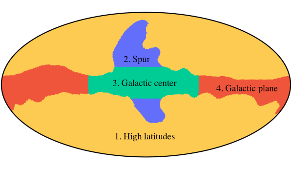
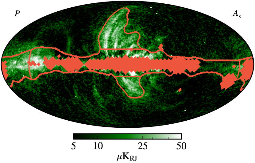
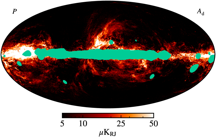
Figure 1: Top: Final region map used in the sampling procedure for the synchrotron spectral index. Middle: Planck 2018 polarized synchrotron amplitude map with the corresponding spectral index processing mask for BeyondPlanck and a region outline that divides the sky into six disjoint regions. This was further reduced to four, motivated primarily by the low signal-to-noise apparent in some of the regions. The mask is chosen to reduce temperature-to-polarization leakage bias, and to exclude bright point sources. Bottom: Planck 2018 polarized thermal dust amplitude with the corresponding processing mask.

The first foreground component, and the brightest Galactic emission mechanism between 30 and 70 GHz, is synchrotron radiation. This emission is generated when relativistic cosmic-ray electrons ejected from supernovae gyrate in the Galactic magnetic field. From both temperature and polarization observations, the synchrotron SED is known to be well approximated by a power-law over several decades in frequency (e.g., Lawson et al. 1987; Reich & Reich 1988; Platania, P. et al. 2003; Davies et al. 2006; Gold et al. 2009), at least from 1 GHz to 100 GHz, although some analyses also claim evidence for a slight spectral steepening towards higher frequencies (Kogut 2012; Jew et al. 2019). The Galprop model (Orlando et al. 2018) is a physically motivated model that takes into account quantities such as the electron temperature ($T_{e}$) and large-scale magnetic field distributions, and this physical model also predicts SED flattening below 1 GHz depending on the model parameters. However, because the flattening occurs at frequencies well below 10 GHz, this is not relevant for the current analysis, which only considers frequencies above 30 GHz, and we therefore assume a straight power-law SED model for synchrotron emission in the following.

Next, several analyses have reported significant spatial variations in $\beta_{\mathrm{s}}$ (e.g., Fuskeland et al. 2014; Krachmalnicoff et al. 2018; Fuskeland et al. 2021). In general, these analyses report flatter spectral indices (around $\beta_{\mathrm{s}}=-2.8$) at low Galactic latitudes, and steeper at high Galactic latitudes (around $\beta_{\mathrm{s}}=-3.1$). This picture appears roughly consistent with similar results derived from intensity observations (e.g., Vidal et al. 2015; Platania et al. 1998; Lawson et al. 1987; Reich & Reich 1988). On the other hand, when analyzing low-resolution WMAP polarization data with full correlated noise propagation, Dunkley et al. (2009) found only minor differences between low and high Galactic latitudes.

Table 1: Overview of all included data bands in the BeyondPlanck polarization analysis. The columns represent the following; 1) Science experiment for that band, 2) frequency band name, 3) data processing pipeline 4) HEALPix resolution in $N_{\mathrm{side}}$, 5) highest included multipole $\ell_{\mathrm{max}}$, 6) beam resolution in arcminutes, 7) bandpass center frequency in GHz, 8) bandpass width in GHz, 9) noise rms given in $\thinspace\mu$K scaled by pixel size, 10) noise format.

Resolution $$\nu_{c}$$ Bandwidth

Experiment Band Processing [GHz] [GHz] K Noise Format

Planck LFI . BeyondPlanck TOD+White noise

Planck LFI . BeyondPlanck TOD+White noise

Planck LFI . BeyondPlanck TOD+White noise

Planck HFI . White noise

WMAP. Ka WMAP Full covariance

WMAP. Q WMAP Full covariance

WMAP. V WMAP Full covariance

As shown in the following, the BeyondPlanck data combination has in general low statistical power to probe spatial variations. We therefore partition the sky into four large disjoint regions, as shown in the top panel of Fig. 1, and fit one spectral index for each region. For reference, the middle panel in this figure shows the Planck 2018 synchrotron amplitude map (Planck Collaboration IV 2018) with region outlines and a corresponding processing mask used in BeyondPlanck.

Since the spectral index is fit uniformly over large sky regions, it is important to impose a processing mask during the posterior evaluation to avoid pixels with poor goodness-of-fit from contaminating surrounding pixels. To this end, we construct a dedicated spectral index processing mask for synchrotron emission by first fitting the component amplitudes given our chosen prior. We then smooth these map to $4^{\circ}$ FWHM, and construct a corresponding mask by thresholding on the strongest 5 % of the signal to remove the brightest part of the Galactic plane. Next, we combine the resulting mask with a smoothed $\chi^{2}$ map thresholded at the strongest 10 % of the signal to remove strong sources such as Tau A and their surrounding area. Finally, we use an un-smoothed $\chi^{2}$ map in order to remove particularly bright compact sources. The resulting mask is visualized along with the region outlines in the middle panel of Fig. 1.

The region set was defined as follows: We started from the 24-region partitioning defined by Fuskeland et al. (2014), which itself was based on the nine year WMAP polarization analysis mask (Bennett et al. 2013). We then ran preliminary analyses to determine the effective posterior width resulting from each region. If this was found to be strongly prior-dominated, we merged neighboring regions. This process resulted in four main regions, which we will refer to as 1) High Latitudes; 2) the Galactic Spur or simply Spur; 3) the Galactic Center; and 4) the Galactic plane. As we will show later, even after this process the high-latitude region does not have sufficient signal-to-noise ratio to significantly constrain $\beta_{\mathrm{s}}$. The reason for this is illustrated in the middle panel of Fig. 1; the synchrotron emission in this region is generally very faint, and there is very little leverage to estimate spectral variations as a function of frequency.

We also note that synchrotron emission is sensitive to Faraday rotation (e.g., Beck et al. 2013) in areas with high electron densities and magnetic fields, which is the case near the Galactic center. This effect is caused by circular birefringence, where left- and right-handed circularly polarized emission traverse the magnetic field of an ionized medium at different velocities, generating a net linear polarization signal with a polarization angle proportional to the field strength. However, since this effect is proportional to the squared wavelength of the radiation, it is most prominent at frequencies below 5 GHz, and it is negligible for most of the sky above 30 GHz. In this paper, we do not make any corrections for Faraday rotation to any frequency channel. However, as shown in Sect. 5, our synchrotron constraints for the Galactic center region are contaminated by systematic effects, and these are most likely due to a combination of instrumental and astrophysical mis-modeling effects.

2.1.2 Thermal dust emission

The second most significant polarized foreground component between 30 and 70 GHz is thermal dust emission generated by interstellar dust grains that collectively account for $\approx$$\thinspace 1\thinspace\%$ of the mass of the interstellar medium; see, e.g., Hensley & Draine (2020) for a recent review of relevant physics and observations constraints. The size of these grains typically varies from a few angstroms to a few tenths of a $\mu\mathrm{m}$, and they are heated up by the interstellar radiation field to a temperature of about 20 K. This heat is then re-emitted thermally with a peak frequency between 1000 and 2000 GHz (as defined in brightness temperature units). Furthermore, due to paramagnetic dissipation resulting from interactions between rotating grains and the local magnetic field, the dust grains tend to align with their short axes parallel to the local magnetic field. In turn, this alignment can induce a polarization signal with a polarization fraction of 20 % or more, as reported by Planck Collaboration XI (2020).

The most commonly used thermal dust SED model in CMB studies is that of a modified blackbody function, as defined in Eq. (7). This SED has three free parameters; 1) the amplitude $\@vec{a}_{\mathrm{d}}$, which traces the surface density of dust particles along each line-of-sight; 2) a spectral index, $\beta_{\mathrm{d}}$, that quantifies the low-frequency slope of the SED, and depends on the physical composition of the dust grains; and 3) the dust temperature, $T_{\mathrm{d}}$, which affects the peak location of the modified blackbody function, and depends on the local radiation field strength at any given position. More complex, and perhaps more realistic, representations do exist, including multi-component modified blackbody (e.g., Finkbeiner et al. 1999; Meisner & Finkbeiner 2015) or physical dust grain models (Guillet et al. 2018).

The particular data combination used in the BeyondPlanck analysis has a very low signal-to-noise ratio for constraining thermal dust SED variations, whether of frequency or spatial origin, as we are working at synchrotron dominated frequencies. In this paper, we therefore only consider one single free parameter for the thermal dust SED, namely a spatially constant value of $\beta_{\mathrm{d}}$. The bottom panel in Fig. 1 shows the Planck thermal dust amplitude map (Planck Collaboration IV 2018) with its corresponding processing mask used in the sampling procedure. This mask was generated by thresholding the $10\thinspace\%$ largest values of the smoothed $\chi^{2}$ map as described in the last section. The thermal dust temperature map is fixed pixel-by-pixel to that derived from Planck temperature observations between 30 and 857 GHz by Planck Collaboration Int. LVII (2020).

No attempts are made to account for SED variations along each line of sight. As emphasized by Tassis & Pavlidou (2015), the sum of two modified blackbodies is not a modified blackbody, and spatial variations in either $\beta_{\mathrm{d}}$ or $T_{\mathrm{d}}$ along each line-of-sight will therefore necessarily break the current model. This effect is particularly important in polarization, since the magnetic field direction also varies along the line-of-sight, potentially resulting in different SEDs for the two Stokes parameters, $Q$ and $U$. However, these variations are far too weak to be measured with the current data set.

3 Data selection

As described by BeyondPlanck (2022), a primary motivation for the BeyondPlanck project is to establish a common analysis platform for past, current, and future CMB observations that supports end-to-end analysis, from raw time-ordered data to final high-level products such as astrophysical component maps and cosmological parameters. To support and guide the algorithm development process, the Planck LFI observations were chosen as a first real-world application for this framework, a choice that was primarily motivated by the fact that this data set is already well known to the collaboration members, and secondarily because of its modest data volume and relatively benign instrumental systematic effects.

At the same time, it is clear that the LFI data are by themselves not able to constrain all relevant astrophysical components. There are at least five significant diffuse components between 30 and 70 GHz; CMB, synchrotron, free-free, AME, and thermal dust emission, while the LFI data only comprise three independent frequency channels. The LFI data must therefore be augmented with external observations in order to derive a statistically non-degenerate model. In principle, the Planck HFI data (Planck Collaboration III 2020) would be an ideal match, providing strong constraints on CMB, free-free and thermal dust emission. However, if these data were to be included the BeyondPlanck analysis in their entirety, they would dominate over the LFI observations in terms of total sensitivity, which would undermine the main purpose of the current presentation, which focuses on the algorithms themselves. For this reason, we choose to include only the Planck HFI 857 GHz channel in temperature and the 353 GHz channel in polarization, to constrain the amplitude of thermal dust emission. In both cases, we adopt the latest rendition of these maps published by the Planck team, as derived by the Planck Data Release 4 (DR4) pipeline, also known as NPIPE (Planck Collaboration Int. LVII 2020).

The same argument applies to the WMAP K-band channel (Bennett et al. 2013). While this channel provides strong constraints on both AME and polarized synchrotron emission, its statistical sensitivity is so high that it would rival that of the Planck LFI 30 GHz channel if included in the BeyondPlanck analysis, which again would undermine the main purpose of the current work. For this reason, we include only the WMAP Ka-, Q-, and V-band channels in the following, centered on 33, 41 and 61 GHz, respectively.

In addition, we include the Haslam 408 MHz survey to constrain synchrotron emission in temperature, see Andersen et al. (2022). This results in a total of eight frequency channels in intensity, and seven frequency channels in polarization, which in principle should be sufficient to constrain a model with five intensity components and three polarization components.

One of the important novel algorithmic developments that will be described in Sect. 4 is true multi-resolution component separation for both linear and non-linear foreground parameters. Specifically, we consider in the following only the low-resolution WMAP polarization data at a HEALPix (Górski et al. 2005) resolution of $N_{\mathrm{side}}=16$, for which dense pixel-pixel noise covariance matrices are available (Bennett et al. 2013). This ensures that we have at least nominally a complete noise description for all frequency channels relevant for CMB extraction, and also that small-scale polarization results are entirely dominated by Planck LFI.

All data except the Planck DR4 353 GHz channel are analyzed as provided by the respective team without any preprocessing or smoothing. The 353 GHz channel, however, is smoothed to an angular resolution of $10{{}^{\scriptstyle\prime}}$ and re-pixelized at a resolution of $N_{\mathrm{side}}=1024$, corresponding to a pixel size of $3\aas@@fstack{\prime}4$. This is done both in order to speed up the analysis process (BeyondPlanck 2022; Galloway et al. 2022), and to suppress small-scale correlated noise which would otherwise lead to a significant $\chi^{2}$ excess. Table 1 provides an overview over all data sets included in the current analysis.

4 Methods

We now aim to fit the data model in Eq. (1) to the data listed in Table 1. We define $\omega=\{g,n_{\mathrm{corr}},\Delta_{\mathrm{bp}},\@vec{a},\beta,\ldots\}$ to be the set of all free parameters in this model of both instrumental and astrophysical origin. Our main goal is then to map out the corresponding joint posterior distribution, which is given by Bayes’ theorem,

$$P(\omega\mid\@vec{d})=\frac{P(\@vec{d}\mid\omega)P(\omega)}{P(\@vec{d})}\propto\mathcal{L}(\omega)P(\omega).$$ (8)

In this expression, $P(\omega\mid\@vec{d})$ is the posterior distribution, and describes our knowledge about $\omega$ after performing the experiment in question; $\mathcal{L}(\omega)\equiv P(\@vec{d}\mid\omega)$ is called the likelihood, and quantifies the information content in $\@vec{d}$ regarding $\omega$; and $P(\omega)$ is called the prior, which quantifies our beliefs regarding $\omega$ before doing the experiment. The prior can also be used actively to regularize specific degeneracies in the model.

This posterior distribution is large and complex with billions of free parameters. Attempting to directly map out the full posterior distribution by brute-force is infeasible. Instead, we resort to Markov Chain Monte Carlo methods, and draw samples from the posterior distribution. In particular, we find that the Gibbs sampling algorithm (Geman & Geman 1984) is particularly well suited to handle the complexity of this model. We therefore adopt the Commander CMB Gibbs sampling framework as the starting point for our analysis. This software was first introduced by Eriksen et al. (2004) for optimal CMB power spectrum estimation applications, building on ideas originally suggested by Jewell et al. (2004) and Wandelt et al. (2004), and later generalized to also account for joint CMB and component separation by Eriksen et al. (2008) and Seljebotn et al. (2019). In this operational mode, Commander played a central role in the official Planck analysis, as summarized by Planck Collaboration I (2014, 2016, 2020) and references therein. BeyondPlanck has now generalized this framework further to also account for low-level TOD processing and mapmaking, effectively turning the entire CMB analysis challenge into one global problem.

4.1 Gibbs sampling

Gibbs sampling formalizes the idea of iterative analysis within a rigorous statistical language. In short, the theory of Gibbs sampling states that samples from a complex joint distribution may be drawn by iteratively sampling from each (typically simpler) conditional distribution. The full BeyondPlanck Gibbs chain (BeyondPlanck 2022) illustrates how this is done in practice, and can be written as

$$\@vec{g} \thinspace\leftarrow P(\@vec{g} \thinspace\mid \thinspace\@vec{d}, \thinspace\xi_{n}, \thinspace\Delta_{\mathrm{bp}}, \thinspace\@vec{a}, \thinspace\beta, \thinspace C_{\ell})$$ (9)

$$\@vec{n}_{\mathrm{corr}} \thinspace\leftarrow P(\@vec{n}_{\mathrm{corr}} \thinspace\mid \thinspace\@vec{d}, \thinspace\@vec{g}, \thinspace\xi_{n}, \thinspace\Delta_{\mathrm{bp}}, \thinspace\@vec{a}, \thinspace\beta, \thinspace C_{\ell})$$ (10)

$$\xi_{n} \thinspace\leftarrow P(\xi_{n} \thinspace\mid \thinspace\@vec{d}, \thinspace\@vec{g}, \thinspace\@vec{n}_{\mathrm{corr}}, \thinspace\Delta_{\mathrm{bp}}, \thinspace\@vec{a}, \thinspace\beta, \thinspace C_{\ell})$$ (11)

$$\Delta_{\mathrm{bp}} \thinspace\leftarrow P(\Delta_{\mathrm{bp}} \thinspace\mid \thinspace\@vec{d}, \thinspace\@vec{g}, \thinspace\@vec{n}_{\mathrm{corr}}, \thinspace\xi_{n}, \thinspace\@vec{a}, \thinspace\beta, \thinspace C_{\ell})$$ (12)

$$\@vec{a} \thinspace\leftarrow P(\@vec{a} \thinspace\mid \thinspace\@vec{d}, \thinspace\@vec{g}, \thinspace\@vec{n}_{\mathrm{corr}}, \thinspace\xi_{n}, \thinspace\Delta_{\mathrm{bp}}, \thinspace\beta, \thinspace C_{\ell})$$ (13)

$$\beta \thinspace\leftarrow P(\beta \thinspace\mid \thinspace\@vec{d}, \thinspace\@vec{g}, \thinspace\@vec{n}_{\mathrm{corr}}, \thinspace\xi_{n}, \thinspace\Delta_{\mathrm{bp}}, \thinspace\@vec{a}, \thinspace C_{\ell})$$ (14)

$$C_{\ell} \thinspace\leftarrow P(C_{\ell} \thinspace\mid \thinspace\@vec{d}, \thinspace\@vec{g}, \thinspace\@vec{n}_{\mathrm{corr}}, \thinspace\xi_{n}, \thinspace\Delta_{\mathrm{bp}}, \thinspace\@vec{a}, \thinspace\beta, \thinspace)$$ . (15)

Here, the symbol $\leftarrow$ means setting the variable on the left-hand side equal to a sample from the distribution on the right-hand side. For convenience, we also define the notation “$\omega\setminus\xi$” to imply the set of parameters in $\omega$ except $\xi$.

The parameters not already introduced are noise power spectrum parameters ($\xi_{n}$), bandpass corrections ($\Delta_{\mathrm{bp}}$), and the CMB power spectrum ($C_{\ell}$). Since the current paper focuses on polarized foregrounds, we are here primarily interested in the amplitude parameters, $\@vec{a}$, sampled in Eq. (13), and the spectral parameters, $\beta$, sampled in Eq. (14). We will therefore describe these two sampling steps in detail in the following, and we refer the interested reader to BeyondPlanck (2022) and references therein for details regarding the remaining steps.

4.2 Signal amplitude sampling

We first consider the signal amplitude conditional distribution, $P(\@vec{a}\mid\@vec{d},\omega\setminus\@vec{a})$, which has already been a primary focus of interest for a long line of studies, including Jewell et al. (2004), Eriksen et al. (2004, 2008), and Seljebotn et al. (2019). In the following, we give a brief summary of these developments, and also highlight two important novel features introduced in the current work.

The appropriate starting point for this conditional distribution is the data model described in Eq. (2). We first note that $\@vec{a}$ contains all signal amplitude maps, using some appropriate linear basis, stacked column-wise, such that $\@vec{a}=[\@vec{a}_{\mathrm{CMB}},\@vec{a}_{\mathrm{s}},\@vec{a}_{\mathrm{d}}]^{t}$, where the $t$ superscript denotes the transpose operator. Further, we adopt a spherical harmonics basis to describe each diffuse component, such that $\@vec{a}_{i}=\{a^{T}_{i,\ell m},a_{i,\ell m}^{E},a_{i,\ell m}^{B}\}$ contains the various temperature and polarization spherical harmonics coefficients (Zaldarriaga & Seljak 1997) for component $i$. Second, for notational convenience we combine the beam and mixing matrix operators in Eq. (2) into one joint linear operator, $\@tens{A}_{\nu}\equiv\@tens{B}_{\nu}\@tens{M}_{\nu}$, such that this equation may be written succinctly as

$$\@vec{m}_{\nu}=\@tens{A}_{\nu}\@vec{a}+\@vec{n}_{\nu}.$$ (16)

Noting that the noise, $\@vec{n}_{\nu}=\@vec{m}_{\nu}-\@tens{A}_{\nu}\@vec{a}$, is assumed to be Gaussian distributed with vanishing mean and a known covariance matrix, $\@tens{N}_{\nu}$, Bayes’ theorem then allows us to write the conditional distribution of interest in the following form,

$$P(\@vec{a}\mid\@vec{d},\omega\setminus\@vec{a}) \propto P(\@vec{d}\mid\omega)P(\@vec{a})$$ (17)

$$\propto P(\@vec{m}\mid\@vec{a})P(\@vec{a})$$ (18)

$$\propto\left(\prod_{\nu}\mathrm{\exp}\left(-\frac{1}{2}(\@vec{m}_{\nu}-\@tens{A}_{\nu}\@vec{a})^{t}\@tens{N}_{\nu}^{-1}(\@vec{m}_{\nu}-\@tens{A}_{\nu}\@vec{a})\right)\right)$$

$$\cdot\mathrm{\exp}\left(-\frac{1}{2}(\@vec{a}-\bar{\@vec{a}})^{t}\@tens{S}_{\nu}^{-1}(\@vec{a}-\bar{\@vec{a}})\right).$$ (19)

Here, the second line holds because TOD binning is a deterministic operation when conditioning on $\omega$ (BeyondPlanck 2022), and the set of binned sky maps, $\@vec{m}$, is a sufficient statistic for $\@vec{a}$; no additional information in the TOD can possibly provide more knowledge about the foreground amplitude maps beyond that stored in $\@vec{m}$ if $\omega$ is exactly known. In the last line we adopt a Gaussian signal prior with mean $\bar{\@vec{a}}$ and covariance matrix $\@tens{S}$, discussed further below. In this paper, we set $\bar{\@vec{a}}=0$, and only use $\@tens{S}$ for smoothing purposes. Since the product of two Gaussian distributions is another Gaussian, $P(\@vec{a}\mid\@vec{d},\omega\setminus\@vec{a})$ is also Gaussian, and the appropriate sampling algorithm is given by a standard multivariate Gaussian, which is discussed in detail in Appendix A in BeyondPlanck (2022). In particular, a proper sample may be drawn by solving the following linear equation for $\@vec{a}$,

$$\biggl{(}\@tens{S}^{-1}+\sum_{\nu}\@tens{A}^{t}_{\nu}\@tens{N}_{\nu}^{-1}\@tens{A}_{\nu}\biggr{)}\thinspace\@vec{a}=\sum_{\nu}\@tens{A}_{\nu}^{t}\@tens{N}_{\nu}^{-1}\@vec{m}_{\nu}+\sum_{\nu}\@tens{A}_{\nu}^{t}\@tens{N}_{\nu}^{-1/2}\eta_{\nu}+\@tens{S}^{-1/2}\eta_{0},$$ (20)

where $\eta_{\nu}$ and $\eta_{0}$ are random Gaussian vectors of independent $N(0,1)$ variates. Because of its large dimensionality, this equation must in practice be solved using iterative linear algebra techniques, and we use a preconditioned conjugate gradient solver for this purpose (e.g., Shewchuk 1994).

This exact equation was discussed in detail by Seljebotn et al. (2019), who also introduced two novel and efficient preconditioners for partial-sky observations based on pseudo-inverse and multi-grid techniques. However, in the present work, for which no analysis mask is imposed during the main Gibbs sampling analysis, we adopt the simpler diagonal pre-conditioner described by Eriksen et al. (2008), which both converges slightly faster with full-sky data, and has a lower computational cost per iteration. The two main novel features regarding Eq. (20) introduced by BeyondPlanck (as described by Andersen et al. (2022) for temperature and by this paper for polarization) concern the data and model representation and active use of spatial priors.

4.2.1 Vector representation and object-oriented programming

Equation  (20) is written in a general vector form, without reference to any specific vector representation or basis, or to any specific form of either the effective mixing matrix, $\@tens{A}_{\nu}$, or noise covariance matrix, $\@tens{N}_{\nu}$. All of these may, in principle, be chosen per component and frequency channel. As detailed by Galloway et al. (2022), we have implemented such flexibility in the most recent version of Commander adopting an object-oriented programming style, where separate classes are defined for each object. For instance, the current implementation contains specific classes for three general types of components, namely diffuse components (for which $\@vec{a}$ is represented in terms of spherical harmonic coefficients, $a_{\ell m}$), point source objects (for which $\@vec{a}$ is represented in terms of a single flux density per compact source), and fixed spatial templates (for which $\@vec{a}$ is represented in a single multiplicative amplitude per template). Any combination of such objects may all be fit simultaneously and jointly through Eq. (20). It is also relatively straightforward to add new types of objects as the need may arise. Two examples of classes that might be important for future applications include pixel- or needlet-based components (e.g., Marinucci et al. 2008), which could be useful for modeling partial sky experiments.

Each of the instrumental objects are also implemented in terms of individual classes. This is particularly relevant for the noise covariance matrix, $\@tens{N}_{\nu}$, which may have very different representations for different experiments. For example, in the current analysis, we model the Planck LFI noise as a sum of correlated and white noise, where the correlated noise is treated as a stochastic variable in the Gibbs chain, and sampled over directly, while the white noise uncertainty is propagated analytically through a diagonal $\@tens{N}_{\nu}$. This approach supports, for the first time, propagation of both correlated and white noise at all angular resolutions. For WMAP, however, we do not yet have access to time-ordered data within our framework, so $\@tens{N}_{\nu}$ is defined in terms of the precomputed dense low-resolution noise covariance matrices provided by the WMAP team (Bennett et al. 2013), which is computationally feasable because this data is smoothed to $N_{\mathrm{side}}=16$. For this reason, WMAP contributes only to large angular scales in the current analysis. Finally, for the Planck 353 GHz measurements, which are essential for modeling polarized thermal dust emission at full angular resolution, we are for now only able to propagate white noise uncertainties with a diagonal $\@tens{N}_{\nu}$ as given by Planck Collaboration Int. LVII (2020). Of course, this will necessarily lead to an underestimation of dust-related uncertainties; hence modeling Planck HFI observations in time-domain is clearly a high-priority issue for future work, but outside the scope of the current project.

In summary, the first critically important novel feature provided by the current Commander implementation is the ability to operate with fundamentally different types of data sets within one analysis and thereby exploit complementary features from each data set to break degeneracies within the full model. At the time of publication, there is direct support for only three types of noise covariance matrices, namely diagonal matrices, WMAP-style dense Stokes $QU$ matrices, and diagonal matrices with explicit marginalization over low-$\ell$ modes. However, using the new infrastructure described here and by Galloway et al. (2022), it is straightforward to add support for other types of matrices. Possibly useful examples include block-diagonal or banded covariance matrices, or noise covariance matrices with specific subspaces projected out through operator based filters. The latter could be particularly useful for ground-based experiments that tend to have limited statistical sensitivity on large angular scales, but high systematic uncertainties. We hope that such features can be implemented, and made publicly available, by third-party authors as Open Source contributions (Gerakakis et al. 2022).

4.2.2 Gaussian spatial priors

The second novel feature supported by the latest Commander implementation is the use of active spatial priors for the diffuse components. For practical purposes, we currently support only Gaussian priors, as described by Eq. (19), as non-Gaussian priors would lead to a prohibitively high computational cost associated with the current conjugate gradient-based approach. In practice, imposing a spatial prior is therefore equivalent to specifying a prior mean, $\bar{\@vec{a}}$, and covariance matrix, $\@tens{S}$, for each component. In the current polarization-oriented analysis, however, we do not wish to enforce any informative priors on any of the three free components (polarized CMB, synchrotron or thermal dust emission), so we set $\bar{\@vec{a}}=0$ for all three. Instead, we use $\@tens{S}$ to adjust the allowed level of fluctuations around zero for each component as a function of angular scale; this is numerically equivalent to choosing an appropriate effective smoothing scale for each component, and might for this paper be considered more of a technical issue than a prior in the normal sense. For an example of an application of active priors, however, see Andersen et al. (2022), in which proper informative spatial priors are imposed on both free-free and anomalous microwave emission.

The remaining question is how to choose a specific form of $\@tens{S}$ for each component. There are two main requirements for this choice. First, $\@tens{S}$ is the covariance of $\@vec{a}$, and therefore dictates the overall fluctuation level of the fitted components. A large value of $\@tens{S}$ implies a weak prior, and the fitted component will then be dominated by the data-driven likelihood term in Eq. (19), while a low value of $\@tens{S}$ implies a strong prior, resulting in values close to the prior mean. In practice, we want the prior to play a limited role where the data have a large signal-to-noise ratio, but a stronger role where the data are noise dominated. It is therefore in general desirable to choose scale-dependent priors, in which the smoothing becomes gradually stronger; the prime example of this is a standard Gaussian smoothing kernel.

As already mentioned, we adopt spherical harmonics as our basis set for $\@vec{a}$, writing each diffuse polarized signal component as

$$a_{X}(\hat{n})=\sum_{\ell m}a^{X}_{\ell m}Y_{\ell m}(\hat{n}).$$ (21)

For each component we therefore also define an angular power spectrum prior of the form

$$\hat{D}^{X}_{\ell}=\left<|a^{X}_{\ell m}|^{2}\right>\thinspace\ell(\ell+1)/2\pi,$$ (22)

where $X=\{E,B\}$. Note that this power spectrum prior representation is conceptually similar to the assumptions made by SMICA (Cardoso et al. 2008), one of the four CMB extraction codes used by Planck.

We adopt the following prior variances for each of the three astrophysical components in the current analysis,

$$\hat{D}^{-1}_{\mathrm{CMB}}(\ell) =0\thinspace\mu\mathrm{K}^{2}$$ (23)

$$\hat{D}_{\mathrm{s}}(\ell) =200\thinspace\mathrm{e}^{-\ell(\ell+1)\sigma^{2}(30{{}^{\scriptstyle\prime}})}\thinspace\mu\mathrm{K}^{2}$$ (24)

$$\hat{D}_{\mathrm{d}}(\ell) =500\thinspace\mathrm{e}^{-\ell(\ell+1)\sigma^{2}(10{{}^{\scriptstyle\prime}})}\thinspace\mu\mathrm{K}^{2},$$ (25)

where $\sigma^{2}(\theta_{\mathrm{FWHM}})\equiv(8\ln 2)\thinspace\pi/(180\cdot 60)\theta_{\mathrm{FWHM}}^{2}$ is the standard deviation of a Gaussian distribution expressed in terms of a full width at half maximum, $\theta_{\mathrm{FWHM}}$, in arcminutes.

Note that for the CMB component, the inverse variance is set to zero, which is equivalent to an infinite variance—or simply no prior at all. For the polarized synchrotron and thermal dust amplitudes, the priors correspond to Gaussian smoothing of $30{{}^{\scriptstyle\prime}}$ and $10{{}^{\scriptstyle\prime}}$ FWHM, respectively. The overall scaling factors are chosen to be 200 and $500\thinspace\thinspace\mu$K², respectively, which correspond to the observed angular power spectrum of each component on large angular scales. In these cases, the priors are used to apodize the resulting foreground amplitude maps with Gaussian smoothing kernels, to avoid ringing around bright sources and the Galactic plane and unphysical degeneracies at high multipoles.

Future analyses may wish to use $\@tens{S}$ to directly estimate the angular power spectrum of each foreground component, fully analogous to the CMB case (Colombo et al. 2022; Paradiso et al. 2022). This will then both alleviate the need of specifying the prior parameters by hand before executing the analysis, and it will ensure optimal smoothing properties for each component, resulting in minimal high-$\ell$ degeneracies between the various components.

Finally, we conclude this section by emphasizing that the above priors are in fact only priors, and not deterministic smoothing operators. Thus, the resulting synchrotron and thermal dust component maps will be determined by the properties of the observed data wherever the data are stronger than the prior. This is important to bear in mind for instance when trying to estimate the angular power spectrum of the resulting maps; the component maps $\@vec{a}$ that result from solving Eq. (20) correspond to a model of the sky without instrumental beam convolution, but with spatially varying noise properties, depending on the local signal-to-noise ratio of the data. The angular resolutions of the synchrotron and thermal dust maps are not given precisely by a Gaussian beam of 30 and 10^′, respectively, but will generally be higher where the data are sufficiently strong. As such, the behavior of these foreground maps is conceptually similar to the GNILC algorithm (Remazeilles et al. 2011), in which a spatially varying angular resolution also results from signal-to-noise ratio variations. Likewise, it is also important to note that the noise properties of these maps are highly non-trivial, and the only statistically robust way of assessing and propagating their uncertainties is through the ensemble of sky map samples produced by the algorithm itself.

4.3 Spectral parameter sampling

The second of the two main conditional distributions discussed in this paper is $P(\beta\mid\@vec{d},\omega\setminus\beta)$, which describes the foreground SED parameters. In general, $\@vec{a}$ and $\beta$ are strongly correlated for a given component, especially for high signal-to-noise data. For temperature-oriented foreground analysis, the BeyondPlanck Gibbs sampler therefore implements a special-purpose sampling step for these parameters, by exploiting the definition of a conditional distribution, $P(\@vec{a},\beta\mid\@vec{d})=P(\@vec{a}\mid\@vec{d},\beta)P(\beta\mid\@vec{d})$ (Stivoli et al. 2010; BeyondPlanck 2022; Andersen et al. 2022). That is, we first sample spectral parameters from the marginal distribution with respect to $\@vec{a}$, and then sample $\@vec{a}$ conditionally with respect to $\beta$. The resulting algorithm is thus effectively an independence sampler in $\{\@vec{a},\beta\}$ (i.e., a sampler where the new proposal does not depend on the previous) with an internally vanishing Markov chain correlation length. In this case, any long-term Markov chain correlations come from degeneracies with other parameters.

However, as described by Stivoli et al. (2010), this algorithm is only computationally practical for observations with the same angular resolution, as the computational expense for evaluating the marginal distribution $P(\beta\mid\@vec{d})$ otherwise becomes prohibitively high. In practice, this means that all data maps must be smoothed to a common angular resolution. For temperature data, this is not a major problem, but for polarization analysis it is non-trivial, since the smoothing operation correlates the instrumental noise. In addition, the data combination used in the current paper involves low-resolution WMAP data with dense noise covariance matrices, and smoothing all data to this resolution is impractical.

Since we focus on polarization in this work, we instead adopt a standard Metropolis-within-Gibbs sampler for $\beta$. In this case, the appropriate conditional posterior distribution may be derived from Eq. (16) by noting that the instrumental noise is assumed to be Gaussian distributed with covariance matrix $\@tens{N}_{\nu}$, and recalling that the amplitude is for the moment assumed to be perfectly known. Therefore,

$$P(\beta\mid\@vec{d},\@vec{a}) \propto P(\@vec{d}\mid\@vec{a},\beta)P(\beta)$$ (26)

$$\propto\Bigg{[}\prod_{\nu} \mathrm{\exp}\left(-\frac{1}{2}\left(\@vec{d}_{\nu}-\@tens{A}_{\nu}(\beta)\@vec{a}\right)^{t}\@tens{N}_{\nu}^{-1}\left(\@vec{d}_{\nu}-\@tens{A}_{\nu}(\beta)\@vec{a}\right)\right)\Bigg{]}P(\beta),$$

where $\@vec{d}=\{\@vec{d}_{\nu}\}$ is the set of all available frequency maps (which within the larger BeyondPlanck framework may be a specific set of frequency map sky samples), and $P(\beta)$ is a user-defined prior, typically a Gaussian distribution with physically motivated mean and standard deviation.

Note that Eq. (26) is also written with a general vector notation, and makes no reference to a specific vector basis for either $\@vec{a}$ or $\beta$; it therefore allows the various data sets to be defined in different basis sets. The only requirement is that there must exist a well-defined mapping between $\beta$ and the effective mixing matrix at each frequency, $\@tens{A}_{\nu}(\beta)$. This generality is precisely what is needed to analyze multi-resolution observations jointly, for instance high-resolution LFI data together with low-resolution WMAP data.

As noted in Sect. 2.1.1, the signal-to-noise ratios of the Planck and WMAP polarization data are modest, so we have defined broad regions for $\beta_{\mathrm{s}}$, as shown in Fig. 1. To sample these values, we employ a standard Metropolis algorithm, as outlined in Algorithm 1, using Eq. (26) as target distribution and a standard symmetric Gaussian proposal distribution, ${T(\beta^{(i)}\mid\beta^{(i-1)})\sim N(\beta^{(i-1)},\@tens{C}_{\beta})}$, where $\@tens{C}_{\beta}$ is a tunable proposal matrix. When evaluating Eq. (26), we first propose $\beta_{\mathrm{s},i}$ independently for each region $i$, and then smooth the resulting map with a $10^{\circ}$ FWHM Gaussian beam to suppress edge effects. This smoothed map is then used to evaluate the mixing matrix $\@tens{A}_{\nu}$ at the appropriate resolution for each frequency channel.

To assess the goodness-of-fit locally across the sky, we compute a $\chi^{2}$ map per pixel. Since WMAP is pixelized with ${N_{\mathrm{side}}=16}$, the $\chi^{2}$ map is too. The sum of this map, after application of an optional analysis mask, is used to evaluate the exponent in Eq. (26) and the corresponding Metropolis acceptance rate.

Initialize $\beta^{(0)}\sim P(\beta)$

for i=$1$, n do

       Propose new index map: $\beta^{\mathrm{prop}}\sim N\left(\beta^{(i-1)},\@tens{C}_{\beta}\right)$

       Compute acceptance rate: $\alpha=\min\left\{1,\frac{P(\beta^{\mathrm{prop}}\mid\@vec{d},\@vec{a})}{P(\beta^{(i-1)}\mid\@vec{d},\@vec{a})}\right\}$

       Draw $u\sim$ Uniform$(0,1)$

       if $u<\alpha$ then

             Accept the proposal: $\beta^{(i)}\leftarrow\beta^{\mathrm{prop}}$

      else

             Reject the proposal: $\beta^{(i)}\leftarrow\beta^{(i-1)}$

      

Algorithm 1 Metropolis algorithm used for spectral index sampling.

As summarized in Algorithm 1, this method has two free tunable parameters, the proposal matrix $\@tens{C}_{\beta}$, and the number of Metropolis steps per main Gibbs iteration, $n$. Before starting a full Gibbs analysis, we perform a tuning run using a diagonal $\@tens{C}_{\beta}$ and adjust the diagonal elements until the resulting accept rate is between 0.2 and 0.8. Once that happens, we run a longer chain with fixed $\@tens{C}_{\beta}$ and replace this matrix with the covariance matrix from the resulting samples. Finally, we run a third chain, computing the Markov autocorrelation length from the resulting chain, and setting $n$ such that the empirical correlation between samples $\beta^{(i)}$ and $\beta^{(i+n)}$ is less than 0.1. These tuning steps are only performed once for each analysis setup, and files are stored on disk for subsequent runs.

4.4 Spectral index priors

The only missing part of the algorithm is now a specification of the priors. For the synchrotron and thermal dust spectral indices, we adopt for the main analysis Gaussian priors of $\beta_{\mathrm{s}}=-3.3\pm 0.1$ and $\beta_{\mathrm{d}}=1.56\pm 0.10$, respectively. The former of these are motivated by the Planck LFI 2018 likelihood analysis, which finds a linear scaling factor of $\alpha=0.058\pm 0.004$ between 30 and 70 GHz. Accounting for the bandpasses of the respective channels (Planck Collaboration II 2020; Svalheim et al. 2022), the quoted scaling factor translates into a spectral index of $\beta_{\mathrm{s}}=-3.3$. The thermal dust spectral index prior is also informed by the official Planck analysis Planck Collaboration X (2016), and in this case the BeyondPlanck data sets do not add any useful independent information to complement the original work, because of the absence of the high signal-to-noise ratio HFI measurements.

Many alternative synchrotron priors were explored during the course of the project, varying both the mean and width. In general, these all led to more significant residuals than the final choice. Regarding the prior width, we note that $\sigma_{\beta}=0.1$ corresponds to only $1\thinspace\sigma$, and the full $3\thinspace\sigma$ confidence interval therefore spans from $-3.6$ to $-3.0$, all of which will be covered during the full Gibbs run. As discussed by Herman et al. (2022), shallower indices than $\beta=-3.0$ are very difficult to accommodate with both LFI and WMAP without introducing an additional low-frequency dust correlated component, for instance polarized AME. Consequently, a broader prior width of $\sigma_{\beta}=0.2$, which permits synchrotron indices as shallow as $\beta_{\mathrm{s}}=-2.7$, leads to large foreground excesses that only can be accommodated by the CMB component within the current model. The result is an obvious foreground bias in the large-scale CMB extraction and a corresponding excess in estimates of the optical depth of reionization (Paradiso et al. 2022). For further discussions regarding different priors, see Sect. 4.2.2.

We treat the four regions differently in terms of synchrotron priors. While the Spur and Galactic plane regions are fitted using both the likelihood and prior as described above, we only include the prior for the high-Galactic and Galactic Center regions. This is because of very strong degeneracies with respect to instrumental systematic effects in these regions. Specifically, the Galactic Center region is particularly susceptible to bandpass mismatch effects, as the bandpass leakage corrections for the 30 GHz channel are of order unity in this region (Svalheim et al. 2022), while the High Latitude region is particularly sensitive to relative gain uncertainties and degeneracies with the CMB quadrupole (Gjerløw et al. 2022). To prevent potential residual systematic errors from contaminating these two regions, we only marginalize over the prior in these cases. While clearly non-ideal, we consider this approach to be preferable to simply fixing the synchrotron index at some given value, as was done for most previous Planck polarization analyses, e.g., Planck Collaboration Int. XLVI (2016). Ultimately, this is a concession that the current data set are not sufficiently strong to uniquely and independently determine both synchrotron and CMB components without priors, and additional measurements from high sensitivity low-frequency experiments such as C-BASS (Jew et al. 2019) and QUIJOTE (Génova-Santos et al. 2015) will be extremely valuable to further improve the quality of the LFI and WMAP data sets in the future.

5 Results

5.1 Goodness-of-fit

Figure 2: Normalized and reduced $\chi^{2}$ per pixel, summed over Stokes $Q$ and $U$ and averaged over all Gibbs samples.

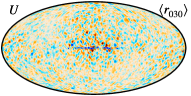
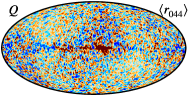
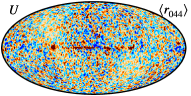
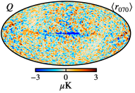
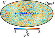
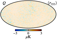
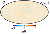
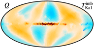
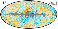
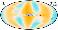
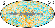
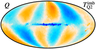
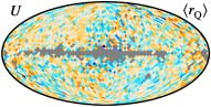
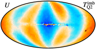
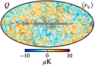
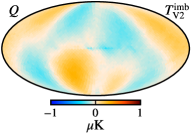
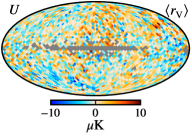
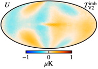
Figure 3: Posterior mean total data-minus-model residual maps ($\@vec{r}_{\nu}=\@vec{d}_{\nu}-\@vec{s}_{\nu}$) in $Q$ and $U$ for BeyondPlanck LFI 30 GHz (top left), 44 GHz (top right), 70 GHz (bottom left) and 353 GHz (bottom right). All maps are smoothed to a common angular resolution of $2^{\circ}$ FWHM.

Figure 4: Posterior mean total data-minus-model residual maps ($\@vec{r}_{\nu}=\@vec{d}_{\nu}-\@vec{s}_{\nu}$) in $Q$ (first column) and $U$ (third column) for all included WMAP bands in the two left-most columns, at $N_{\mathrm{side}}=16$, masked with the processing mask applied in the pipeline. The second and fourth columns show corresponding transmission imbalance template maps for one of the differencing assemblies (eg. Q{1,2}, V{1,2}) per residual as derived by Jarosik et al. (2007); note that these templates are each associated with an unknown scaling amplitude that may take either sign.

Before turning our attention to the final astrophysical products, we assess the goodness-of-fit of the fitted sky model. Our first statistic is the total $\chi^{2}$ per pixel, summed over frequencies and Stokes $Q$ and $U$ parameters and averaged over Gibbs samples, as shown in Fig. 2. To aid visual interpretation, this map is plotted in the form $(\chi^{2}-n_{\mathrm{dof}})/\sqrt{2n_{\mathrm{dof}}}$, where $n_{\mathrm{dof}}=20\thinspace 798$ is an estimate of the total number of degrees of freedom (i.e., number of full-frequency data pixels summed over frequencies, minus the number of fitted parameters.) within each $N_{\mathrm{side}}=16$ pixel. If the model performs as expected, this quantity should have zero mean and unit standard deviation. Overall, we see that our model appears to perform well at high Galactic latitudes, while the Galactic plane shows clear excess $\chi^{2}$. This behavior is not surprising, as the Galactic Center is far more complex and difficult to model, both in terms of astrophysics and instrumental effects. We do note that the morphological structure of the excess $\chi^{2}$ appears to be correlated with Galactic emission, rather than instrumental effects.

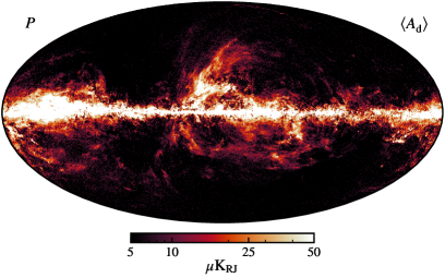
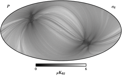
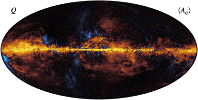
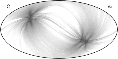
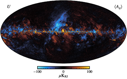
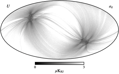
Figure 5: (Left column:) Polarized thermal dust amplitude maps, plotted in terms of the polarization amplitude $P=\sqrt{Q^{2}+U^{2}}$ (top row) and the Stokes $Q$ (middle row) and $U$ parameters (bottom row). (Right column:) Corresponding posterior standard deviation maps. All maps are evaluated at a reference frequency of 353 GHz in units of $\thinspace\mu$K_RJ, and averaged over all available Gibbs samples. The effective angular resolution is $10\arcmin$ FWHM.

Another useful statistic for evaluating the model goodness-of-fit is data-minus-model residual maps per frequency, ${\@vec{r}_{\nu}=\@vec{d}_{\nu}-\@vec{s}_{\nu}}$. These residual maps provide a visual summary of remaining systematics on a band-to-band basis, which is useful when physically interpreting specific artefacts in the $\chi^{2}$ map. Figure 4 shows such residual maps for the Planck frequency bands, smoothed to $2^{\circ}$ FWHM to suppress white noise. Generally, these maps indicate excellent model performance, with amplitudes of $\lesssim\thinspace$$3\thinspace\mu$K. High Galactic latitudes appear consistent with noise, while small deviations are seen around the Galactic Center, with a morphology that may suggest residual bandpass-induced temperature-to-polarization leakage (Paradiso et al. 2022).

The 44 GHz channel exhibits the largest relative variations. This is expected from algorithmic arguments, by noting that this channel does not dominate the determination of any single fitted astrophysical component. In contrast, the 30 GHz channel dominates synchrotron determination; the 70 GHz channel dominates CMB determination; and the 353 GHz channel dominates thermal dust determination. As such, any excess fluctuations in these channels will rather be interpreted as signal belonging to whichever foreground component that uses this as a reference band. For component separation purposes, it is clearly advantageous to have multiple frequency maps with comparable signal-to-noise ratio per astrophysical component, as instrumental artefacts are then much easier to identify. Employing the full set of Planck frequency maps in a future analysis will improve these results, and provide many more internal cross-checks. However, we once again stress that the main aim of the current study is not to present a new state-of-the-art sky model, but rather to demonstrate the BeyondPlanck algorithm.

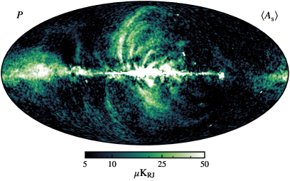
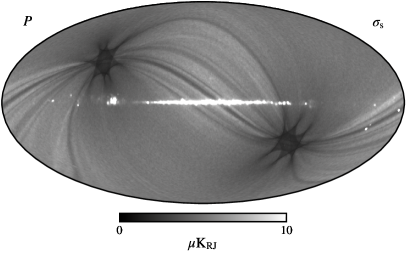
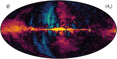
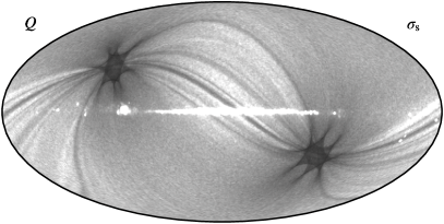
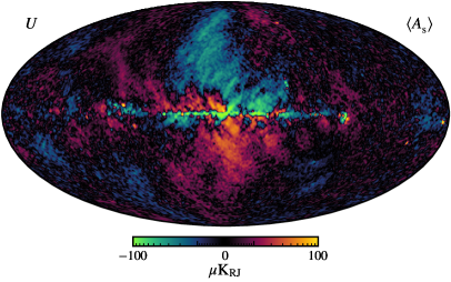
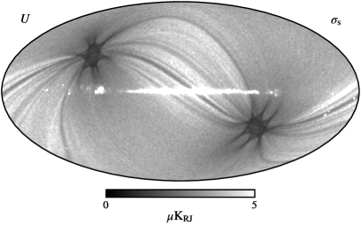
Figure 6: Same as Fig. 5, but for polarized synchrotron emission evaluated at 30 GHz. In this case, the effective angular resolution is $1^{\circ}$ FWHM.

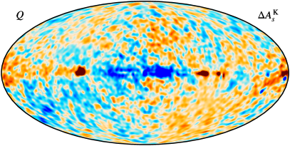
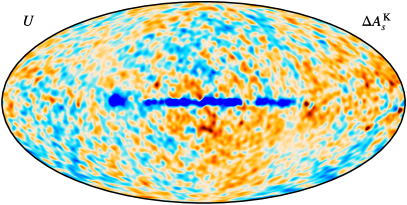
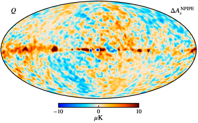
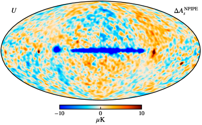
Figure 7: (Top panel:) Difference between the BeyondPlanck polarized synchrotron amplitude and the raw WMAP $K$-band map (Bennett et al. 2013), the latter being scaled to 30 GHz assuming a spectral index of $\beta_{s}=-3.1$. (Bottom panel:) Similar difference between the BeyondPlanck and Planck DR4 (Planck Collaboration Int. LVII 2020) synchrotron amplitude maps. Left and right columns show Stokes $Q$ and $U$ parameters respectively, and all maps are smoothed to a common angular resolution of $3^{\circ}$ FWHM.

\begin{overpic}[width=433.62pt]{figs/sampletrace_P_synch-beta_pixreg_val_t3.pdf} \put(83.0,15.5){\includegraphics[scale={0.4}]{figs/UF_sindex_new_map2_T_w8_n1024_c-Plotly-9_v2.pdf}} \end{overpic}

Figure 8: Synchrotron spectral index as a function of Gibbs iteration for an analysis that includes nine disjoint regions (see inset sky map). The prior is in this case $\beta_{\mathrm{s}}=-2.8\pm 0.1$, and all regions are constrained using the full posterior distribution.

Figure 4 shows the remaining residual maps, i.e., WMAP Ka, $Q$, and $V$-band. In all three cases, we see coherent large-scale structures that are clearly morphologically inconsistent with instrumental noise. These residual maps appear visually similar to the set of correction templates presented by Jarosik et al. (2007) that account for known transmission imbalance between the A- and B-sides of the WMAP instrument, as shown in the second and fourth column of Fig. 4. In our study, we do not apply any explicit corrections for these templates; hence, they appear in the frequency residual maps. However, they are accounted for in the WMAP covariance matrices, and the corresponding modes are therefore appropriately down-weighed when fitting the astrophysical parameters with Eqs. (20) and (26). Transmission imbalance effects will therefore not bias any astrophysical results, but only result in larger uncertainties. At the same time, these residual maps clearly suggest how a future joint time-domain processing of WMAP and Planck will be able to constrain the WMAP transmission imbalance parameters with high precision. Once that happens, the corresponding spatial modes will no longer need to be algebraically projected out, as is effectively done now, but may rather be used for scientific inference, on the same footing as any other mode. This work has already started, and preliminary results are discussed by Watts et al. (2022).

5.2 Amplitude results

We now turn our attention to the astrophysical results, and start with the posterior amplitude maps, $\@vec{a}$. First, Fig. 5 shows the thermal dust amplitude, plotted at an angular resolution of $10\arcmin$ FWHM at $N_{\mathrm{side}}\thinspace$=$\thinspace 1024$ for the polarization amplitude ${P=\sqrt{Q^{2}+U^{2}}}$, as well as $Q$ and $U$ averaged over an ensemble of Gibbs samples. The right column shows the corresponding posterior distribution standard deviation per pixel, with values peaking around $3\thinspace\mu$K_RJ. As mentioned in the previous subsection, the thermal dust amplitude is for all practical purposes determined by the pre-computed HFI 353 GHz band in the BeyondPlanck processing, and the LFI bands have little influence. As a result, the thermal dust standard deviation maps shown in Fig. 5 are essentially given deterministically by the input 353 GHz standard deviation map. These uncertainties are underestimated in the Galactic plane, where systematic effects must be significant. Overall, the polarized thermal dust amplitude map is in good agreement with previous results.

Figure 6 shows corresponding results for the polarized synchrotron amplitude map. At high Galactic latitudes, we see that the standard deviation of this component traces the LFI 30 GHz scanning strategy, and is correspondingly largely determined by instrumental white noise. However, in this case the Galactic plane is in fact dominated by temperature-to-polarization leakage due to bandpass and gain uncertainties, resulting in a morphology that matches the 30 GHz intensity map.

In Fig. 8, we show Stokes parameter maps of the difference between the BeyondPlanck map of polarized synchrotron amplitude and two independent synchrotron tracers. The top panel shows differences with respect to the full WMAP $K$-band frequency map at $23$ GHz. To account for its different effective frequency, we scale the $K$-band map according to a power-law model with $\beta_{\mathrm{s}}=-3.1$, or, explicitly, by a factor of 0.38. The two data sets appear to agree reasonably well, with a certain degree of diffuse large scale structure. Considering that the effective frequency difference between $K$-band and 30 GHz is only $7$ GHz, spatial variations in the synchrotron spectral index are unlikely to be relevant, as a difference of $\Delta\beta_{\mathrm{s}}=0.02$ only translates into approximately $0.5\thinspace\mu$K in the relevant regions.

The bottom panel of Fig. 8 shows similar difference maps with respect to the polarized synchrotron amplitude map derived from Planck DR4 (Planck Collaboration Int. LVII 2020). In this case, the high-latitude residuals are dominated by the Planck scanning strategy, with an overall morphology that closely matches the LFI gain residual template produced by Planck Collaboration II (2020) and discussed by Gjerløw et al. (2022) in a BeyondPlanck context. At the same time, no striking correlations are seen between the $K$-band and Planck DR4 residual maps, and the overall levels of variation in these two difference maps are comparable.

5.3 Spectral index results

\begin{overpic}[width=433.62pt]{figs/sampletrace_P_synch-beta_pixreg_val.pdf} \put(83.0,22.0){\includegraphics[scale={0.4}]{figs/UF_sindex_4regions_T_w8_n1024_c-Plotly-4.pdf}} \end{overpic}

Figure 9: Synchrotron spectral index as a function of Gibbs iteration binned using the final BeyondPlanck analysis configuration with four disjoint regions and a prior of $\beta_{\mathrm{s}}=-3.3\pm 0.1$. Dotted lines indicate regions that are sampled exclusively from the prior distribution, while solid lines indicate regions that are sampled from the full posterior distribution.

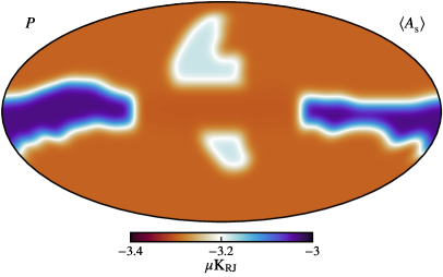
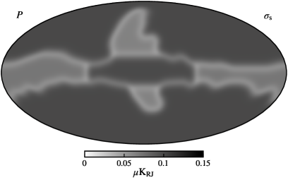
Figure 10: Posterior mean (left panel) and standard deviation (right panel) maps of the spectral index of polarized synchrotron emission. Note that a prior of $\beta_{\mathrm{s}}=-3.3\pm 0.1$ is applied to all four regions, but only the Galactic Spur and Galactic Plane regions are constrained with data through the likelihood; see Sect. 5.3.2 for further discussion.

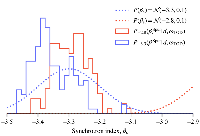
Figure 11: Normalized histogram of synchrotron spectral index ($\beta_{\mathrm{s}}$) for the Spur region using two different priors. The solid lines show the marginal distribution of spectral index values without TOD sampling using a prior (dotted lines) of $\beta_{s}=-2.8$ (red), and $\beta_{s}=-3.3$ (blue).

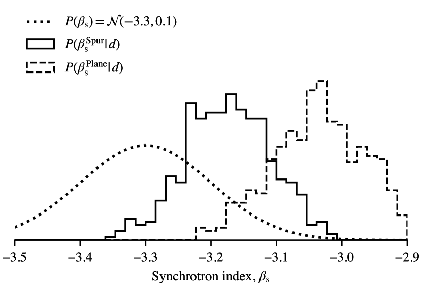
Figure 12: Normalized histogram of synchrotron spectral index ($\beta_{\mathrm{s}}$) for the Spur and Plane regions over the 500 ensemble Gibbs samples, with corresponding prior, $P(\beta_{s})$.

5.3.1 Spectral index regions

Before presenting the synchrotron spectral index posterior distribution, we revisit the final choice of sampling regions and priors by considering a preliminary analysis configuration with nine disjoint regions rather than four, and a spectral index prior of $\beta_{\mathrm{s}}=-2.8\pm 0.1$, rather than $\beta_{\mathrm{s}}=-3.3\pm 0.1$. The results are summarized in Fig. 8, which shows $\beta_{\mathrm{s}}$ as a function of iteration for a Gibbs chain that explored only the $\{\@vec{a},\beta\}$ sub-space. That is, all TOD-related parameters were kept fixed in this particular run, in order to highlight the conditional signal-to-noise ratio of the foreground sector. Each region is labeled with its corresponding posterior mean and standard deviation after a burn-in period of 25 Gibbs samples, and accompanied by a color-coded region map for visualization purposes.

Starting with the most visually striking result, we see that the Galactic Center region immediately converges to a very low mean value of $\beta_{\mathrm{s}}=-4.15\pm 0.05$, well outside the range of previously reported values. Of course, we already know that this region is associated with high $\chi^{2}$ values (see Fig. 2), and in particular shows clear evidence of temperature-to-polarization leakage when compared to WMAP and Planck DR4 (see Fig. 8). Rather than letting these systematic errors potentially contaminate other parameters through an unphysical synchrotron spectral index fit, we instead assign the spectral index of this region a physically meaningful value, as defined by the prior. However, we do not fix it, but rather draw a new value from the prior in every sample, and thereby marginalize over the prior. Technically speaking, this is done by omitting the likelihood term in Eq. (26) when computing the Metropolis acceptance probability.

Next, we see that the Gum Nebula region also converges to a notably low value, and this is most likely related to the same $\chi^{2}$ excess that is seen for the Galactic Center. Furthermore, we note that the Gum Nebula region, as outlined in Fig. 1, exhibits very little synchrotron signal and is therefore particularly prone to residual systematic bias when applying weak prior constraints.

Most of the remaining regions fluctuate around values that are at least nominally consistent with previous analyses reported in the literature. We do note, however, that the two Southern Hemisphere regions return values that are high, at $\beta_{\mathrm{s}}=-2.70\pm 0.07$ and $\beta_{\mathrm{s}}=-2.88\pm 0.07$, respectively, while most of the remaining ones lie around $\beta_{\mathrm{s}}\approx-3.1$. Thus, even when measured conditionally with respect to the TOD parameters, there is slight evidence of a positive bias of $\Delta\beta_{\mathrm{s}}\approx 0.1$ or more with respect to the Northern Hemisphere. Returning once again to Fig. 1, we see that all high-latitude regions exhibit very low signal-to-noise ratio, as the instrumental noise is comparable to, or dominates over, the synchrotron amplitude in most pixels. These regions are therefore all particularly susceptible to residual systematic errors and/or prior volume effects (e.g., Dunkley et al. 2009). Indeed, when sampling jointly over the full range of time-ordered systematic corrections, we find that these regions converge to $\beta_{\mathrm{s}}\gtrsim-2.5$. As in the case of the Galactic Center, we do not take this as evidence for a truly flatter spectral index in these regions, but rather as an indication that there are low-level residual systematics present in either BeyondPlanck, WMAP, or Planck DR4 353 GHz (or, possibly, all of them) at a level that is sufficient to bias the spectral index in the faintest regions.

We conclude that dividing into nine sky regions is sub-optimal (not to mention 24, which was the starting point of the analysis; see Sect. 2.1.1), as most regions do not have sufficient signal-to-noise ratio to independently constrain $\beta_{\mathrm{s}}$, so they are highly susceptible to residual systematic uncertainties. In particular, small changes in the absolute calibration can introduce confusing CMB dipole leakage at high latitudes, while bandpass variations can cause problems near the Galactic Center.

We therefore reduce the number of disjoint regions, and combine the four high Galactic latitude regions into one, and we merge all regions along the galactic plane, except for the Galactic center. Even in this minimal configuration, the high Galactic latitude region is not well constrained, and we therefore sample this from the prior alone, as for the Galactic Center. This leaves only two regions (the Galactic Spur and the Galactic Plane) to be sampled properly with the full posterior distribution, and, fortunately, both of these appear to be both signal-dominated and stable with respect to instrumental parameter variations.

5.3.2 Synchrotron spectral index results

We are now finally ready to present the main results of this paper, namely constraints on the synchrotron spectral index. Starting with the individual Gibbs samples, Fig. 9 shows traceplots for each of the four regions. The first half shows the first Gibbs chain, and the second half shows the second Gibbs chain, both after discarding 10 samples for burn-in. Overall, we see that the correlation length is modest, as in 30–50 samples. The chains mix well, and appear at least visually to be statistically stationary; it is not easy to identify the point at which the two chains are joined, which typically is the case if there are long-term drifts. For completeness, Fig. 10 shows posterior mean and standard deviation sky maps evaluated from these chains.

We also see that the Spur and Galactic Plane regions, which are the only two regions for which $\beta_{\mathrm{s}}$ is actually fitted, have shallower mean spectral indices than the prior of $\beta_{\mathrm{s}}=-3.3$. This may seem somewhat paradoxical, since it is then natural to ask why the prior was not set to $\beta=-3.1$. As discussed earlier, the reasons are two-fold. Firstly, the High Latitude region actually does appear to prefer a steeper spectral index, as indicated by the Planck likelihood analysis (Planck Collaboration V 2020), AME constraints (Herman et al. 2022), and our own preliminary studies. At the same time, this region is also both the most important region for CMB purposes, and it is prior-dominated. It is therefore particularly important that the prior works well for this region. Secondly, the prior only has a very mild effect on the two signal-dominated regions anyway, precisely because of their higher statistical weight. This is explicitly demonstrated in Fig. 11, which compares conditional distributions for the Spur region with two different priors centered on $\beta=-3.3$ (blue) and $-2.8$ (red), respectively. (In this case, the TOD parameters are kept fixed, and the $P(\@vec{a},\beta|\@vec{d},\omega_{\mathrm{TOD}})$ distribution is explored for one arbitrarily chosen realization of $\omega_{\mathrm{TOD}}$.) Here we see that shifting the prior mean by as much as $\Delta_{p}\beta=0.5$ only affects the posterior by $\Delta\beta\lesssim 0.1$. For a more realistic possible prior shift of $\Delta_{p}\beta=0.2$, the final posterior shifts will be $\Delta\beta\lesssim 0.03$, which is small compared to the overall variations seen in Fig. 9. In short, the Spur and Galactic plane regions are signal-dominated, and the prior is of limited importance.

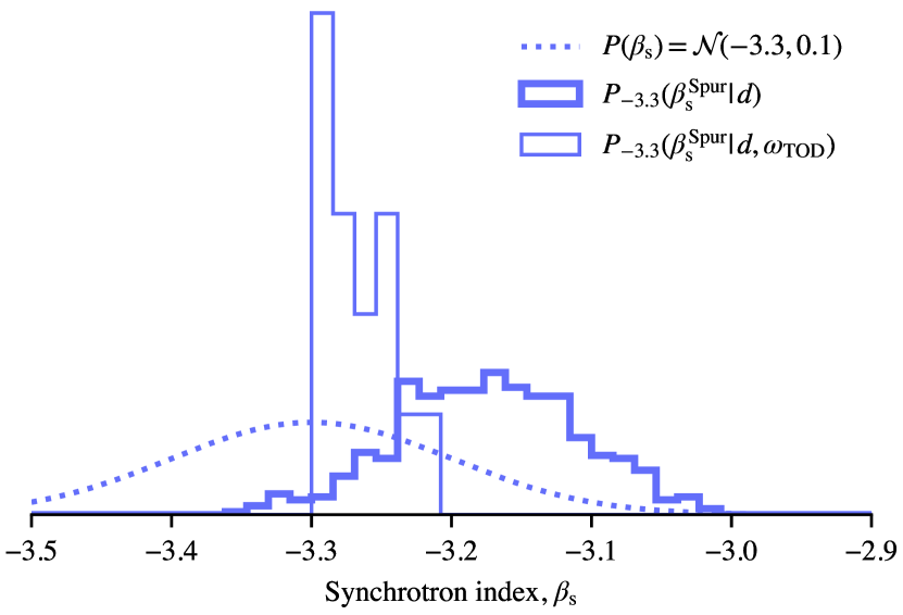
Figure 13: Normalized histogram of synchrotron spectral index ($\beta_{\mathrm{s}}$) for the Spur region using a prior of $\beta_{s}=-3.3$. The bold line shows the full BeyondPlanck posterior distribution including TOD sampling, and the thin line shows the corresponding posterior distribution when conditioning on TOD parameters.

Figure 12 compares the posterior distributions for these two regions. For these, we find posterior mean and standard deviations of ${\beta_{\mathrm{s}}^{\mathrm{Spur}}=-3.17\pm 0.06}$ and ${\beta_{\mathrm{s}}^{\mathrm{Plane}}=-3.03\pm 0.07}$. Both of these values are consistent with earlier constraints in the literature, that suggests a steepening of the spectral index from low to high latitudes (e.g., Fuskeland et al. 2021; Krachmalnicoff et al. 2018). Similarly, Dunkley et al. (2009) reports a variation of $\Delta\beta_{\mathrm{s}}=0.08$ between low and high Galactic latitudes using the WMAP data, while we find a variation of $\Delta\beta_{\mathrm{s}}=0.14$ between the Galactic plane and the Spur using both WMAP and LFI data. The steepening is however only statistically significant at the $2\thinspace\sigma$ level as determined in the current analysis.

Next, to illustrate the importance of marginalization over TOD parameters, Fig. 13 compares the full marginal posterior distribution (thick blue histogram) with a similar posterior distribution that fixes the TOD parameters at one arbitrary Gibbs sample (thin blue histogram). Thus, the former marginalizes over the full BeyondPlanck data model, while the latter only marginalizes over foreground parameters and white noise. The relative widths of the two distributions clearly demonstrates the importance of accounting uncertainties in the full parameter sets, and correspondingly also the advantage of joint global parameter estimation.

As an additional validation of these results, we replace the three BeyondPlanck-processed LFI frequency map samples with the corresponding preprocessed Planck DR4 maps (Planck Collaboration Int. LVII 2020). In this case, we find spectral indices of ${\beta_{\mathrm{s}}^{\mathrm{Spur}}=-3.20\pm 0.06}$ and ${\beta_{\mathrm{s}}^{\mathrm{Plane}}=-3.06\pm 0.06}$, respectively, which are individually statistically consistent with the BeyondPlanck results at the $0.5\thinspace\sigma$ level.

5.3.3 Thermal dust spectral index

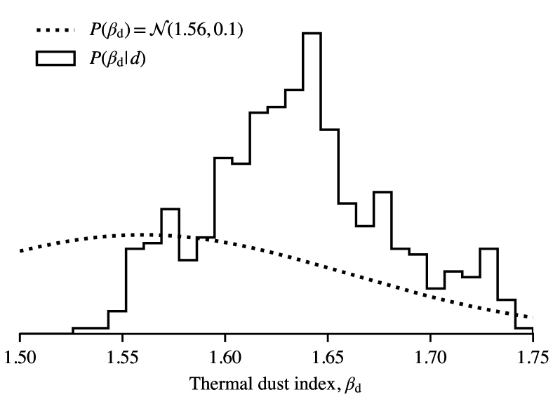
Figure 14: Normalized histogram of thermal dust spectral index ($\beta_{\mathrm{d}}$) over the 500 ensemble Gibbs samples, with corresponding prior.

For polarized thermal dust emission, we fit only one power-law index, $\beta_{\mathrm{d}}$, across the full sky, while fixing the dust temperature on the latest Planck estimate (Planck Collaboration Int. LVII 2020). This is exclusively due to a limited signal-to-noise ratio, and not a statement regarding the complexity of the true sky. In this case, we adopt a prior of $\beta_{\mathrm{d}}=1.56\pm 0.10$, motivated by the most recent Planck HFI results (Planck Collaboration IV 2018; Planck Collaboration Int. LVII 2020).

The resulting posterior distribution is shown in Fig. 14, which may be reasonably approximated as a Gaussian with $\beta_{\mathrm{d}}=1.62\pm 0.04$. This mean value is thus slightly steeper than expected based on HFI, with a statistical significance of about $1.5\thinspace\sigma$. Furthermore, the uncertainty is significantly smaller than the prior width, which suggests that the result is indeed data-driven, even when marginalizing over the full BeyondPlanck instrument model.

While we caution against over-interpreting the significance of this result, we do note that a possible spectral steepening in the thermal dust SED around 100 GHz would have dramatic consequences for future high-sensitivity $B$-mode experiments. Thus, understanding whether this result is due to a statistical fluke, or instrumental modeling errors (for instance, because of an overly simplistic bandpass correction model), or actual astrophysics is an important goal for future analysis. Including Planck HFI frequencies between 100 and 217 GHz in a future analysis will clearly be informative in this respect.

6 Summary and conclusions

The two main goals of this paper are to introduce a Bayesian sampling algorithm for polarized CMB foreground models as embedded within the end-to-end BeyondPlanck framework, and to present the first results from this pipeline as applied to the Planck LFI data set. This is the first time a joint global parametric model that accounts for both instrumental and astrophysical parameters has been fit to the Planck LFI data within a single joint posterior distribution, allowing for seamless end-to-end error propagation. This is also the first time a joint analysis of the Planck LFI and WMAP data has resulted in physically meaningful spectral indices for both polarized synchrotron and thermal dust emission. This analysis thus paves the way for future analyses that should integrate and analyze more data sets.

Indeed, we stress that the current analysis configuration has been specifically designed to demonstrate the properties and performance of the algorithm itself, not to derive a new best-fit sky model. Specifically, critically important data sets, such as WMAP $K$-band and Planck HFI, have been intentionally omitted, precisely because of their high signal-to-noise ratios; if they had been included, the results would have been dominated by WMAP and HFI methodology. Including these data sets, and other important ones like C-BASS (Jew et al. 2019) or QUIJOTE (Génova-Santos et al. 2015) will be done in future work, either by members within the current BeyondPlanck team or by external researchers, and either by starting from time-ordered or from pre-pixelized sky maps. In many respects, the current analysis configuration may very possibly represent one of the most difficult challenges that the BeyondPlanck pipeline will face, since it is the least constrained; future analyses will always have access to more data, and the resulting sky models will therefore be less degenerate.

With that important caveat in mind, particularly notable highlights from the current analysis include the following:

1. We constrain the spectral index of polarized synchrotron emission, $\beta_{\mathrm{s}}$, in two large and disjoint regions of the sky, covering the Galactic Spur and the Galactic Plane, with best-fit values $\beta_{\mathrm{s}}^{\mathrm{Spur}}=-3.17\pm 0.06$ and $\beta_{\mathrm{s}}^{\mathrm{Plane}}=-3.03\pm 0.07$, respectively. These results are statistically consistent with previous WMAP-only results (Dunkley et al. 2009). The current analysis finds some evidence for spatial variation between spur and plane in $\beta_{\mathrm{s}}$, but only statistically significant at the $2\thinspace\sigma$ level. At the same time, we note that the high Galactic latitude region has a too low signal-to-noise ratio to support any robust conclusions regarding $\beta_{\mathrm{s}}$, while the Galactic Center region exhibits too strong residual systematic effects.

2. We constrain the spectral index of thermal dust emission between 30 and 70 GHz to $\beta_{\mathrm{d}}=1.62\pm 0.04$, which is somewhat steeper than that previously reported by Planck HFI (Planck Collaboration IV 2018; Planck Collaboration Int. LVII 2020) of $\beta_{\mathrm{d}}\approx 1.56$, but still statistically consistent.

3. Through joint analysis of the Planck and WMAP data, we have been able to isolate and highlight the effect of transmission imbalance in the WMAP observations. This strongly suggests that a future joint analysis of Planck and WMAP data in the time-domain will be able to constrain the WMAP transmission imbalance parameters to high accuracy. This work has already started, as discussed by Watts et al. (2022).

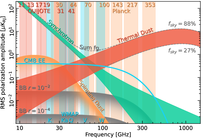
Figure 15: Polarization amplitude root-mean-square (RMS) as a function of frequency and astrophysical component and polarized emission. Each component map is smoothed to a common angular resolution of $1^{\circ}$ FWHM, and the lower and upper edges of each band are defined by the RMS outside masks covering $27\thinspace\%$ and $88\thinspace\%$ of the sky, respectively. An artificial broadening has been applied to the low-amplitude tails of the foreground spectra to visually indicate uncertainties in low signal-to-noise regions for the relevant components. The $EE$ CMB spectrum is generated from ideal CMB simulations based on the best-fit Planck $\Lambda$CDM model, while the $BB$ limits are derived with tensor-to-scalar ratios of $r=10^{-2}$ and $10^{-4}$, respectively. Additionally, we visualize an upper limit on the polarization fraction of spinning dust of 1 % as has been reported in literature (Génova-Santos et al. 2017; Macellari et al. 2011; Herman et al. 2022).

Figure 15 provides an overview of the main polarized microwave components in the frequency range from 10 to 1000 GHz, as described by the posterior BeyondPlanck results and our assumed sky model with the addition of spinning dust with a polarization fraction of 1 % (Génova-Santos et al. 2017; Herman et al. 2022). Here, each component is represented in terms of the standard deviation of the polarization amplitude evaluated over 88 % (top edge of each band) and 27 % (bottom edge of each band) of the sky, with all WMAP and Planck frequency bands marked as vertical columns. To illustrate the importance of detailed foreground modeling and error propagation, the predicted levels of CMB $BB$ power for tensor-to-scalar ratios of $r=10^{-2}$ and $r=10^{-4}$ are marked by diffuse gray regions. In order to achieve a significant measurement of this signal, exquisite control over both foreground contamination and systematic effects and their interplay will be quintessential. We believe that the analysis framework presented in this paper, and in a suite of companion papers, can play an important role in this work, by providing a common and statistically well-defined analysis platform for past, current and future CMB experiments.