On mathematical aspects of evolution of dislocation density in metallic materials
Abstract.
This paper deals with the solution of delay differential equations describing evolution of dislocation density in metallic materials. Hardening, restoration, and recrystallization characterizing the evolution of dislocation populations provide the essential equation of the model. The last term transforms ordinary differential equation (ODE) into delay differential equation (DDE) with strong (in general, Hölder) nonlinearity. We prove upper error bounds for the explicit Euler method, under the assumption that the right-hand side function is Hölder continuous and monotone which allows us to compare accuracy of other numerical methods in our model (e.g. Runge-Kutta), in particular when explicit formulas for solutions are not known. Finally, we test the above results in simulations of real industrial process.
Key words and phrases:
delay differential equation; metallic materials; Euler method; Runge-Kutta method; strict error analysis1. Introduction
Numerous models of materials developed in the second half of the 20th century use external variables as independent ones [18]. The model output is a function of some process parameters (e.g., strain, temperature, strain rate), which are external variables and which are grouped in the vector (, where is the model output). The main drawback of this approach is that it does not properly take into account the history of the considered process. Namely, within these models once the conditions of the process change, the calculated material responses immediately by moving to a new equation of state and the model output is a function of new values of external variables. On the other hand, it was observed experimentally, see for example [21], that metallic materials in general show delay in the response to the change in processing conditions. Therefore, the rheological models, which include internal variables as independent parameters, were proposed in the literature. In the internal variable approach (IVM) the model output is a function of time ; again of some process parameters (e.g., temperature, strain rate), which we grouped in the vector and internal variables, which we grouped in the vector : (so now ). Since the internal variables remember the state of the material, these models give more realistic description of materials behavior.
The model with one internal variable, which is the average dislocation density , is usually considered for metallic materials. The model follows fundamental works of Kocks, Mecking, and Estrin [5, 15]. Main assumptions of this model are repeated briefly below. Since the stress during plastic deformation is governed by the evolution of dislocation populations, a competition of storage and annihilation of dislocations, which superimpose in an additive manner, controls a hardening. Thus, the flow stress accounting for softening is proportional to the square root of dislocation density
| (1.1) |
where is a material dependent coefficient, is stress due to lattice resistance or solution hardening, is length of the Burgers vector, and is shear modulus (e.g. see [18, chapter 3.3]).
The evolution of dislocation populations is controlled by hardening (, where is the strain rate) and restoration () processes. During deformation the dislocation density increases in a monotonic way until the state of saturation is reached. However, at elevated temperatures an additional softening mechanism called recrystallization occurs. The term recrystallization is commonly used to describe the replacement of a deformation microstructure by new grains [14]. Processes of phase changes (transformations), which are common in metallic materials, compose nucleation and growth stages. It means that during this process the two phases can coexist. Recrystallization is classified as a specific type of the transformation, in which the part of the material with increased dislocation density due to deformation is considered an old phase and the part of the material with rebuilt microstructure and free of dislocations is considered a new phase. Two types of the recrystallization can be distinguished, dynamic which occurs during the deformation and static, which occurs after the deformation. The final microstructure and mechanical properties of the alloys are determined, to a large extent, by the recrystallization. The research on the recrystallization dates back to 19th century, and the fast development of the dynamic recrystallization theory was summarized in [14]. The most recent research on this process is described in [10]. A lot of factors have a significant effect on the recrystallization, including the stacking fault energy, the process conditions (temperature, strain rate), the grain size and few other metallurgical parameters. Modeling of recrystallization has been for decades based on the Johnson-Mehl-Avrami-Kolmogorov model, which is based on the external variables only and gives erroneous results when process conditions are changed. In the present work an approach based on the internal variable, which is a dislocation density, was proposed. Since various parts of the material during recrystallization can be in a different state and this process is launched when certain threshold of the accumulated energy is reached, the rate of this process depends on the history of the energy accumulation. The energy accumulated in the material in the form of dislocations from the past acts as the driving force for the current progress of the recrystallization. Similarly, the driving force during static recrystallization depends on the energy accumulated earlier in the material during deformation. This process is launched when certain threshold of the accumulated energy is reached and the rate of this process depends on the history of the energy accumulation. In the mathematical description of this phenomenon a delay differential equation is a natural tool. This approach appeared first in [4]. For more details, see Chapter 3.3 in [18].
From the above reasoning, it turns out that the evolution of dislocation populations accounting for hardening, recovery, and recrystallization is given by
| (1.2) |
where as before is time, is the strain rate, are model parameters (sometimes time independent, but in most of real world cases dependent on other process parameters, such as , etc.), and are additional model coefficients. The function is responsible for the delay in the response to the change in processing conditions, and in the most of practical considerations it is enough to consider
| (1.3) |
In what follows, we will always use in the form (1.3) in (1.2). In what follows, by a solution of (1.2) we mean any continuous function , which we assume everywhere with the only possible exception at the point , where one-sided derivatives may disagree.
The rate of hardening is inversely proportional to the length of the Burgers vector and the free path for dislocations , that is when and when . The recovery and the recrystallization are temperature dependent processes following the Aarhenius law [13]. The average free path for dislocations , the self-diffusion parameter , and the grain boundary mobility in equation (1.2) are calculated as
| (1.6) |
| (1.7) | |||||
| (1.8) |
where: is self-diffusion coefficient, is activation energy for self-diffusion, is coefficient of the grain boundary mobility, is activation energy for grain boundary mobility, is austenite grain size, , is the Zener-Hollomon parameter, is activation energy for deformation, is the universal gas constant equal to J/mol, and , are auxiliary model coefficients. Note that in real industrial process even varies in time, so coefficients are complicated functions changing in time.
Critical dislocation density for recrystallization is calculated as
| (1.9) |
where , , are coefficients, and is the time between beginning of deformation and beginning of recrystallization (i.e. the moment of reaching ). Note that depends on which also changes in time. In simplified approach, will be constant, but in practice it is not. In any case, we are interested in the first time that this value is reached (curves representing and intersect), which is by the definition value of .
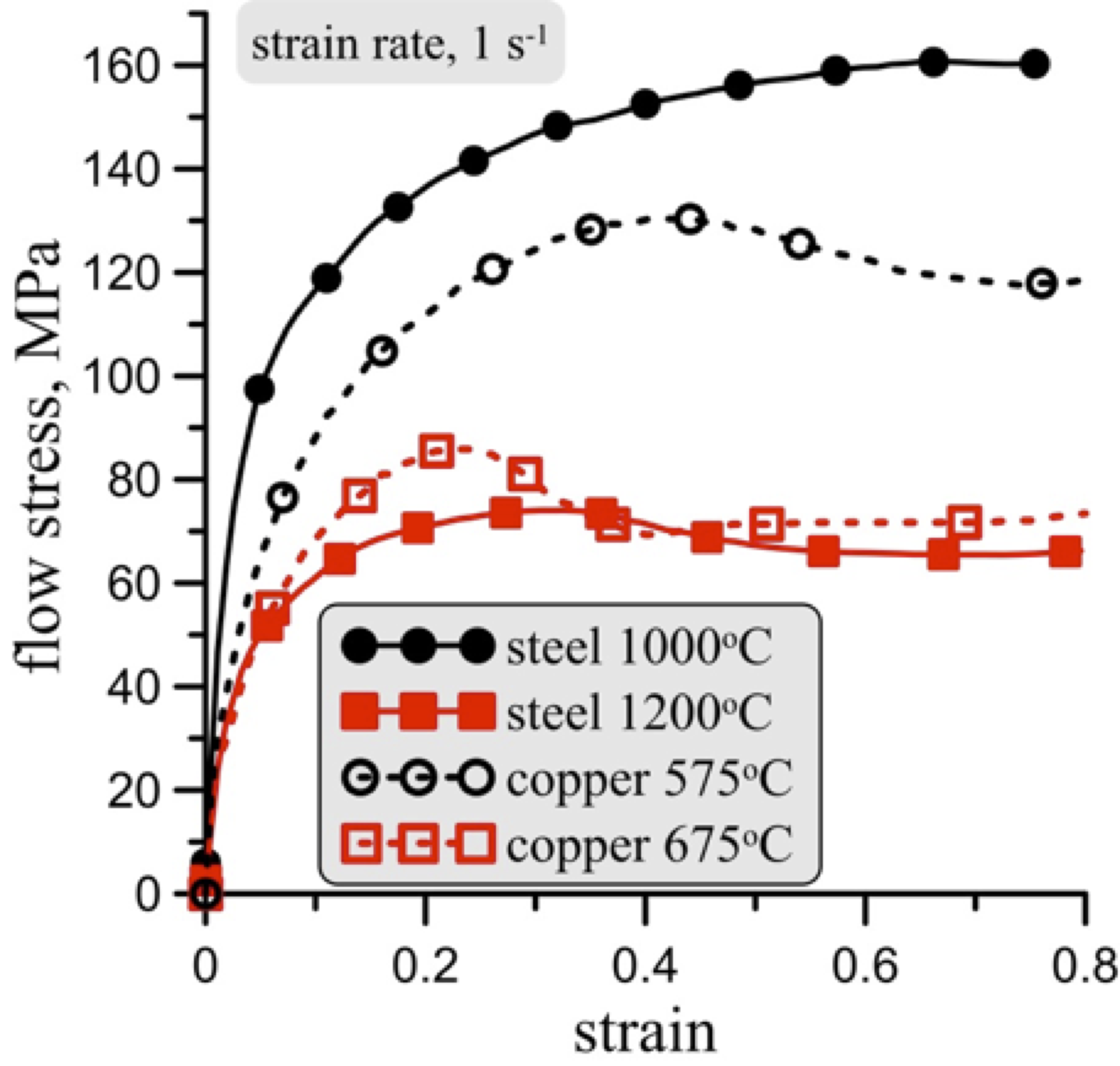
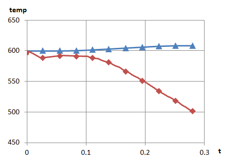
In real world, measurement of dislocation density during the process is difficult. Fortunately, flow stress can be measured, and it is dependent on the dislocation density, which evolution is given by equation (1.2). Measurements of flow stress from experiments for different materials are presented in Figure 1.
Besides numerical simulations, we will perform a detailed theoretical analysis of (1.2), and there are a few good reasons to do that. First of all, it is hard to find in the literature mathematical tools that can be directly applied to this type of equations, while in recent years some studies of its numerical evolution were undertaken. Classical literature for ordinary differential equations, e.g. [2, 9], assumes some regularity of right-hand side function, commonly Lipschitz condition. Similar assumptions occur for delay differential equations, cf. [1, 19]. Unfortunately, there is no strict mathematical analysis of the error even in the case of standard numerical methods like explicit Euler method, for considered here nonlinear delay differential equations with a locally Hölder continuous and monotone right-hand side function. In our opinion it is valuable to show that results of these simulations reflect the real behavior of the system. Fortunately, analytic solutions and rigorous formulas can be used for numerical tests on this equation for simplified equations derived from (1.2), especially the cases when coefficients are no longer time (or other process parameters) dependent. As a result of this study we want to ensure that numerical methods, which are accurate at one hand, and have low computational cost at the same time. As we will see, there are good candidates here (as we prove they behave well for simplified models).
While nowadays there is high popularity in methods of higher order (e.g. Runge-Kutta scheme), they are not suitable for our needs. First of all, observe that in (1.2) the right-hand side function is only monotone and locally Hölder continuous, however it is not differentiable at and it is not even globally Lipschitz continuous (recall that the global Lipschitz condition is usually imposed in the literature). Yet another problem in the case of delayed equations, is that in practice in the case of higher order we will need value of delayed function in points not used in mesh of computation. This leads to interpolation of these values, possibly canceling effect of higher order, and making precise error analysis extremely problematic. Taking all the above reasons into account, we decided to stick with classical Euler scheme whose correctness and suitability we are convinced both numerically and mathematically. In particular, we provide in Theorem 3.2 the error bounds for the classical Euler scheme under such irregular assumptions. Moreover, numerical results reported in Section 4 confirmed its good behavior, when applied to the equation (1.2) with real-world parameters. For further numerical experiments in real-world setting we refer the reader to our recent paper [16].
The paper is organized as follows. Section 2 is devoted to existence and uniqueness of solutions of (1.2). Section 3 contains error behavior analysis for explicit Euler method with some discussion why we finally chose it for our main numerical experiments. Finally, in Section 4 some numerical results are given, with simulations for (1.2) with real world parameters of selected metallic materials (copper and Dual Phase steel, DP steel for short) at the end.
2. Existence and uniqueness of solutions of some instances of (1.2)
In this section we will consider (1.2) with some relatively mild additional conditions on time-dependent coefficients and (mainly that they are bounded, end extremal values satisfy some relations bonding them together). Before we can prove main results of this section, we will consider the following auxiliary delay differential equation obtained by simplification of (1.2) to the form
| (2.1) |
where and are constant. Observe that in (2.1), compared to (1.2), we assume constant strain rate , and by convention function is given by (1.3). Properties of this simplified equation will allow us to approximate evolution of (1.2).
2.1. Existence and uniqueness of solution
We start with presenting two auxiliary results on (2.1), which will help us to analyze (1.2). Note that the case is very similar to the simple delayed equation considered in [6]. Unfortunately, we may not use directly formulas of solutions from there, since in our case of (2.1), influence of delayed term is also delayed by characteristic function in (1.3). In [6] it was pointed out that too large value of with respect to can result in unbounded oscillations and as a result negative values of . In what follows we will see that the condition always prevents it, while as reported in [6], cases may lead to unstable solutions. The situation in this case is much dependent on the value of , however. The analysis of (2.1) will lead to analogous conditions on coefficients in (1.2). However as we will see later, our model (with real world parameters) will satisfy these assumptions. The following result is an adaptation of the proof of Theorem 3.2. in [19] to delay differential equations (2.1). The argument is standard, however, we present it for the reader’s convenience.
Lemma 2.1.
Let be a noncontinuable solutions of delay differential equations (2.1) and assume that . Then .
Proof.
There is such that . But then we can view as a noncontinuable solution of the ODE defined for :
If was bounded, then by standard argument for ODEs (e.g. see [8, Theorem 2.1]) can be continued beyond which is a contradiction. ∎
Lemma 2.2.
Assume that and . The solutions of delay differential equations (2.1) with the initial-value condition
exist for any and are bounded by .
Proof.
It is easy to verify that for the solution exists, is increasing and contained in the interval . After reaching , discontinuity in the vector field disappears, and (2.1) becomes standard delay differential equation with continuous initial condition, defined by solution of (2.1) on the interval
In the case that there is a solution that cannot be continued on it must leave the interval first, see Lemma 2.1. Denote
and assume that . It is clear that and there is a decreasing sequence , such that , is well defined (i.e. is in domain of ) and .
By definition . Let us consider two cases.
-
(1)
Assume first that . If then for for sufficiently small which is impossible, because for small , is continuous on contradicting the choice of sequence .
Let us assume now that . This implies that there exists such that for function defined by for and for is continuous. But then, the function is a solution of the ODE with continuous vector field defined by for and for , with initial condition . It is clear that as a solution of that equation must satisfy because for the vector field is negative. Therefore, for we have . This is in contradiction with the choice of sequence .
-
(2)
Assume next that . There is such that for we have . But then, for all these we have a lower bound for the values of the vector field
showing that is an increasing function on the interval . A contradiction again.
Indeed, the solution of (2.1) is bounded and contained in , which then implies that it can also be continued onto , see Lemma 2.1. ∎
While we state the following result for in practice we will be interested only in . The proof is standard, we leave details to the reader.
Lemma 2.3.
Assume that and . The solutions of delay differential equations (2.1) and with initial-value condition
exist for any and are bounded by .
Remark 2.4.
In the following theorem we may replace by and by . This way it can be applied to a slightly larger class of equations.
Remark 2.5.
In practice, the value of temperature is much higher than and by physical constraints also bounded from the above. So if then and as a consequence all the coefficients are bounded and separated from zero.
Theorem 2.6.
Assume that there are positive constants and such that coefficients (for each ; this takes into account other process parameters that these coefficients are dependent) and for every . Additionally assume that and either or . Then the solutions of delay differential equations (1.2) with the initial-value condition
exist for any and are bounded by and are unique.
Proof.
Consider the following equations with constant coefficients:
| (2.2) |
and with initial-value condition for all and
| (2.3) |
and with initial-value condition for all where is provided solution of (1.2), provided it exists. In the other case we omit delay term in (2.2) and (2.3). By Lemmas 2.2 and 2.3 solutions of (2.2) and (2.3) exist for every and while . In fact, when despite of relations between other coefficients. Simple calculations yield that for we have and which implies that exists for and and this inequality can be recursively extended onto further intervals which completes the proof of boundedness of solutions.
Consider time interval for . We may view on each of these intervals as ODE. Let
where on each of the above intervals delay term can be regarded as a function of but independent of solution. In fact we can view as a function defined for all by putting for all . This way we may regard (1.2) as associated ODE
| (2.4) |
with initial condition , since values for have already been determined. It is obvious that . Note that there are such that for we have , so in particular is bounded away from , provided it is defined. We already know that there is a solution of (1.2) (so also (2.4)) in and assume that is another solution in , but with the same initial value as , i.e., . Then we have
| (2.5) |
since for all the function is nonincreasing (recall for all ), hence
| (2.6) |
Repeating the above arguments inductively on consecutive intervals we complete the proof. ∎
Remark 2.7.
In practical applications, the condition will not be usually satisfied. The reason is that inside the metallic material usually it will take some time to observe . However after some time, say we will have for all and at the same time will not diverge too much from . The reader may check that in these cases, statements of Theorem 2.6 are still valid.
The same reasoning can be applied to other coefficients.
2.2. Some solutions of the toy model (2.1) and existence of
For the equation (2.1) we can give explicit formula for solution in the case when . For the fractional values of it is rather hard to provide analytic formulas. On the other hand, we may view the above two cases of as bounds for intermediate values. The main utility of these formulas, is that they can be used to strict control of error in preliminary numerical experiments. As usual, let us assume that
| (2.7) |
Under the assumption above the solution attains the critical value in finite time , and it is not hard to check that
| (2.8) |
Namely, for the equation (2.1) is reduced to a simple linear equation with the solution
| (2.9) |
which is a strictly increasing function and . In the intervals , , we solve the equation (2.1) recursively as follows. Let us denote by the solution in the interval ( in is given by (2.9)). We have two cases:
-
(i)
: The solution with the initial value is
(2.10) for .
-
(ii)
: The initial value leads to the solution
(2.11) where
(2.12)
Note that both solutions are given in integral form, which most likely is impossible to present as explicit functions in the case , since we have doubly exponential terms under integral. For the case it seems possible to provide some formulas (similarly to [6]), however their complexity increases rapidly with multiplies of , mainly because vector field is discontinuous.
On the other hand, equations (2.10) and (2.11) can be treated with numerical integration with rigorous control of numerical errors. This way we can accurately estimate numerical errors of numerical solutions of these equations (e.g. by explicit Euler method). This gives us a chance for rigorous comparison of various numerical methods for solving equations of type (2.1), possibly ensuring similar behavior of numerical approximations of its further generalizations.
Remark 2.8.
The assumption that seems to be crucial in order to have a nontrivial problem, since, in the case when , we get by (2.7) that and . Moreover, the equation (2.1) becomes the following Bernoulli equation
| (2.13) |
which, under the initial value , has the following trivial solution for all and all . By Theorem 2.3 all solutions of (2.1) tend to the zero solution when . Hence, only the case when is of practical interest. It is worth mentioning, that it is always the case in considered models.
Unfortunately in applications we cannot assume that coefficients are time independent. Then the question arise to which extent the new equation is similar. The first step will be to show that critical time , under certain assumptions on , always exists also in that case. Assume that assumptions of Theorem 2.6 are satisfied, in particular coefficients as well as are bounded, i.e. and for every .
Consider time-dependent version of (2.1) before reaching derived from (1.2) with “smallest possible” vector fiels, that is the equation (stated for )
| (2.14) |
Hence
| (2.15) |
which is clearly continuous and positive function on , and since both are bounded away from zero, we also have
| (2.16) |
Therefore solution of both (2.15) and (1.2) satisfy
In particular, when then there exists such that the solution of (2.14) satisfies (and by continuity we may assume that is smallest among all such times).
For example, let us consider the equation (1.2) with , time independent but positive , continuous and, as before, assume that for all . Hence, we are considering time-dependent version of (2.1), with , and . Under the assumption (2.7) we have, by the above considerations, that there always exists , since in that case . Moreover, it can be shown that
| (2.17) |
where is the inverse function for , which exists since is strictly increasing. Note that in the case when we restore from (2.17) the equation (2.8). Nevertheless, only in this particular case we know the closed formula for . In general the nonlinear equation has to be solved numerically.
As long as is calculated, we can repeat arguments presented earlier in Section 2.2 and provide formulas for solutions when . As before, for , , we solve the equation (2.1) with time-dependent recursively. Let us denote by the solution in the interval , where in is given by
| (2.18) |
We consider the following two cases:
-
(i)
: Then for , , the solution is given by
(2.19) where
(2.20) -
(ii)
: Then for , , the solution is
(2.21) where
(2.22)
Despite, the formulas being slightly more complicated, they can be effectively used within the process of evaluation of accuracy and correctness of numerical methods used to solve time-dependent versions of (2.1).
3. Error analysis of the explicit Euler method
Since in the case when the exact formulas for the solution of (1.2) are not known, we use the suitable numerical methods to approximate on a finite time interval. We are interested in the error analysis for solutions of (1.2) after reaching , since delay activates at this point. This approach will allow us to impose some reasonable assumptions on continuity of vector field. It will be visible in assumptions (F1)-(F4) below; see also Remark 3.7.
We consider the (general) delay differential equation
| (3.1) |
with a given right-hand side function and where for .
For fixed the explicit Euler method that approximates a solution of (3.1) for is defined recursively for subsequent intervals. Namely, let and
where
| (3.2) |
Note that is uniform discretization of the subinterval . Discrete approximation of in is defined by
| (3.3) | |||||
| (3.4) |
Let us assume that the approximations , , have already been defined in the interval (for it was done in (3.3) and (3.4)). Then for we take
| (3.5) | |||||
| (3.6) |
as the approximation of in .
In this section we present rigorous analysis of the error of the explicit Euler method under the nonstandard assumptions on the right-hand side function of the equation (3.1). Namely, we assume that is monotone and locally Hölder continuous instead of the global Lipschitz continuity. According to the authors knowledge, there is lack of such analysis in the literature (cf. [1, 2, 9]), since we consider a non-Lipschitz case.
Let us emphasize once again, that we cannot apply higher order methods under out assumptions (such us Runge-Kutta schemes), since we do not assume that function is differentiable. Observe that indeed it is the case of our main equation (1.2), since the right-hand side function of (1.2) is not differentiable at when .
For the right-hand side function in the equation (3.1) we impose the following assumptions:
-
(F1)
.
-
(F2)
There exists a constant such that for all
-
(F3)
For all ,
-
(F4)
There exist , such that for all ,
In the following fact we provide an example of the right-hand side function that satisfies the assumptions (F1)-(F4). In what follows we use this function in order to approximate the solution of (1.2) in the case when , see also Remark 3.7. The proof of this fact is standard and we leave it to the reader.
Lemma 3.1.
Let the functions satisfy Hölder condition with the Hölder exponent and with the Hölder constant , and define a function as follows111 if and if
| (3.7) |
If the functions are bounded in , then the function satisfies (F1)-(F4) with , , , and .
The following theorem is the main result of this section. It states the upper bound on th error of the Euler algorithm under the mild assumptions (F1)-(F4). We want to underline here that up to our knowledge there are no such results in the literature, since in standard situation at least the global Lipschitz condition is satisfied. Unfortunately, due to the form of the main equation (1.2), this condition is not satisfied, which supports necessity of the following result.
Theorem 3.2.
We want to underline here that the theorem above gives the error estimates for the Euler scheme on the fixed and bounded time horizon . This is crucial, since the discretization parameter depends on .
In order to prove Theorem 3.2 we need several auxiliary lemmas. Note that the same symbol may be used for different constants.
Lemma 3.3.
Let us consider the following ordinary differential equation
| (3.10) |
where , and satisfies the following conditions:
-
(G1)
.
-
(G2)
There exists such that for all
-
(G3)
For all ,
Then the equation (3.10) has a unique solution in ,
| (3.11) |
and for all
| (3.12) |
where .
Proof.
Since the right-hand side function is continuous and it is of at most linear growth (i.e. (G1) and (G2) are satisfied), Peano’s theorem guarantees existence of the solution (e.g. see Theorem 70.4, page 292 in [7]). The uniqueness follows from the monotonicity condition (G3). Namely, let us assume that (3.10) has two solutions and with the same initial-value . Then for all
Therefore, the mapping is non-increasing and we get for all
which, together with continuity of , implies that for all .
The following result provides an upper bound on the error of explicit Euler method applied to ODEs with monotone and Hölder continuous right-hand side functions.
Lemma 3.4.
Let us consider the following ordinary differential equation
| (3.14) |
where , and satisfies the following conditions:
-
(G1)
.
-
(G2)
There exists such that for all
-
(G3)
For all ,
-
(G4)
There exist and such that for all ,
Let us consider the explicit Euler method based on equidistant discretization. Namely, for we set , , , and let be such that . We take
| (3.15) |
Then the following holds.
-
(i)
There exists such that for all we have
(3.16) -
(ii)
There exists such that for all we have
(3.17)
Proof.
We have that
| (3.18) |
and . Hence, by the discrete version of Gronwall’s lemma we get that for all
| (3.19) |
where . This proves (3.16).
For we consider the following local ordinary differential equation
| (3.20) |
By (3.19) we get for all that
| (3.21) |
and by the Gronwall’s lemma we obtain
| (3.22) |
where . Therefore, for all
| (3.23) |
with . Now, we have that
| (3.24) |
for . Note that for all , due to the assumption (G3), the following holds
| (3.25) | |||||
Hence, we arrive at
| (3.26) |
We now estimate the second term in (3.24). We have by (3.15), (3.19), (3.20), (3.22), (G4), and (3.23) that
| (3.27) |
where . Since , , we obtain that
| (3.28) |
where .
In the following lemma we show, by using the results above, that the delay differential equation (3.1) has unique solution under assumptions (F1)-(F3). Note that the assumptions are weaker than those known from the standard literature. Namely, we use only monotonicity and local Hölder condition for the right-hand side function .
Lemma 3.5.
Proof.
We proceed by induction with respect to .
For , the equation (3.1) can be written as
| (3.35) |
with the initial condition . Denoting by
| (3.36) |
we get, by the properties of , that ,
| (3.37) |
with , and
| (3.38) |
Therefore, by Lemma 3.3 we get that there exists a unique continuously differentiable solution of the equation (3.35), such that
where
and for all
where
depends only on .
Let us now assume that there exists such that the statement of the lemma holds for the solution . Consider the equation
| (3.39) |
with the initial condition . Let
| (3.40) |
We get by the inductive assumption and from the properties of that , for all we have
| (3.41) |
with , and
| (3.42) |
Hence, again by Lemma 3.3 we get that there exists a unique continuously differentiable solution of the equation (3.39), such that
where
and for all we have
where .
From the above inductive construction we see that the solution of (3.1) is continuous. Moreover, due to the continuity of , , and we get for any that
Hence, the solution of (3.1) is continuously differentiable.
The proof is completed. ∎
Lemma 3.6.
Proof.
Conditions (i), (ii), and (iii) follow by Lemma 3.5.
By the assumption (F4) and Lemma 3.5 we get for all , that
∎
Now we are ready to prove Theorem 3.2.
Proof of Theorem 3.2.
On the interval we approximate the solution of (3.1) by the explicit Euler method
| (3.44) | |||||
| (3.45) |
where . Applying Lemmas 3.6 and 3.4 to , , , we get that
| (3.46) |
where , and
| (3.47) |
where .
In we consider the following differential equation
| (3.48) |
with the initial value and . We approximate (3.48) by the auxiliary Euler scheme
| (3.49) | |||||
| (3.50) |
By (3.46) we have that
| (3.51) |
Applying Lemmas 3.6, 3.5 and 3.4 to , , , we get that
| (3.52) |
and
| (3.53) |
where that, in particular, depends on the initial value of the equation (3.1). Let us denote by
where we have that . From (3.50) and (3.6) we have for that
| (3.54) |
where
and
From (3.54) we obtain that
which, together with the assumption (F3), implies
| (3.55) |
Moreover,
hence
| (3.56) |
Since for , we have that
| (3.57) |
Recall a well known fact that for all and it holds
| (3.58) |
Then by the assumption (F4), Lemma 3.5 and (3.46) we have the following estimates
| (3.59) |
where , and
| (3.60) |
Furthermore, it holds that for all
where and . By using discrete Gronwall’s inequality we obtain
| (3.61) |
Therefore, by (3.61) and (3.60) we obtain for all
| (3.62) |
with independent of . From (3.57), (3.59), and (3.62) we get for sufficiently large and that
| (3.63) |
where are independent of . Solving this discrete inequality yields
| (3.64) |
with independent of . Since
by (3.53) and (3.64), we arrive at
| (3.65) |
with independent of .
On the consecutive intervals we proceed by induction. Namely, let us assume that there exist and such that
| (3.66) |
and
| (3.67) |
(For the statement has already been proven in (3.65) and (3.61).) In the interval we consider the following ODE
| (3.68) |
with the initial value and . We approximate (3.68) by the following auxiliary Euler scheme
| (3.69) | |||||
| (3.70) |
By (3.66) we have that
| (3.71) |
Repeating the arguments used from (3.48) to (3.65), but now for , , , , we obtain
| (3.72) |
and
| (3.73) | |||||
and
| (3.74) |
with independent of , provided that is sufficiently large. This ends the proof. ∎
Remark 3.7.
In Lemma 3.1 we provided an example of a function that satisfies (F1)-(F4). Note that , with , coincides in with
| (3.75) |
which is a right-hand side function of the main equation (1.2) for where represents the delay term . Knowing that the solution of (1.2) is unique and non-negative (see Theorem 2.6), the solutions of (1.2) and
| (3.76) |
coincide for . (We take for .) This justifies, why we can use the Euler scheme in order to approximate the nonnegative solution of (1.2).
4. Numerical experiments
In this section we will provide numerical simulations of (1.2) with real world parameters. However, before we do so, we will take a closer look to (2.1), that is we assume that and are time independent. This will give us a preliminary insight into possible evolution of (1.2). In particular we will see how it changes with the change of parameters , in particular influence of the boundary condition . We will also check how the accuracy of solutions changes with time step, and comment of empirical speed of convergence of numerical solutions.
It is also worth mentioning that (2.1), while much simplified compared to (1.2), has its utility for modeling of our process. Namely, it can be used in inverse analysis, as laboratory experiments are usually done in controlled environment. In particular and can be assumed constant in laboratory experiments, which leads to time-independent coefficients .
4.1. Empirical tests of convergence - selected instances of equation (2.1)
As before, we divide our discussion into two cases when .
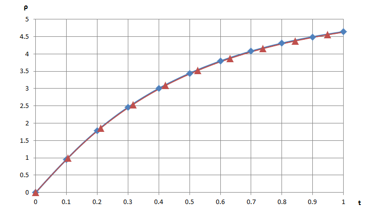
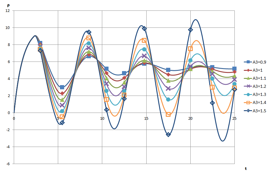
In the case when , we consider four sets of parameters (see Figure 2)
-
(i)
,
-
(ii)
,
-
(iii)
.
All solutions are considered on the interval . Initial conditions on all particular intervals are given by values of corresponding analytical formula.

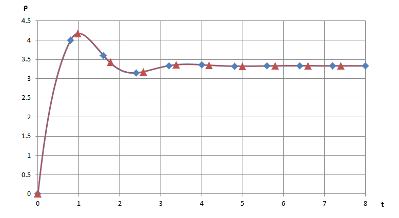
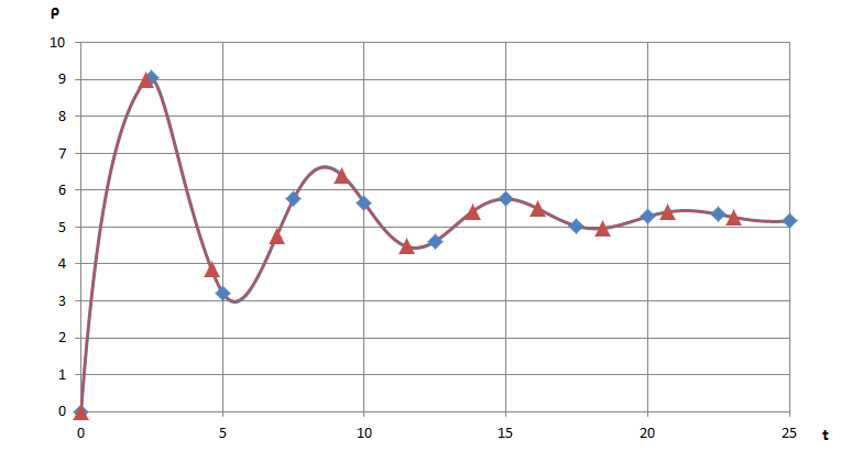
We also considered case with parameters range showing influence of violated condition (see Figure 3):
-
(iv)
, ,
-
(v)
, .
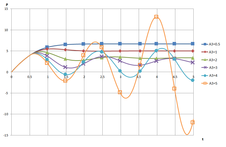
Note, that in these cases or we even have . Let us emphasize, that the assumptions of Theorem 2.2 are broken. Nevertheless, the derived methods work properly what suggests that the assumptions might be weakened in further research. Notice however, that while solutions exists (and can be computed), it is hard to find their technological justification (recall that represents dislocation density, so Figure 3(v) definitely cannot represent real technological process). Note that similarly to effect observed in [6] for equation similar to the case , large (or large ) may lead to unbounded oscillations of solutions and technologically unjustified solutions. In fact, as we can see, such solutions may occur even when solution stabilizes (i.e. oscillations are bounded and decreasing in amplitude).
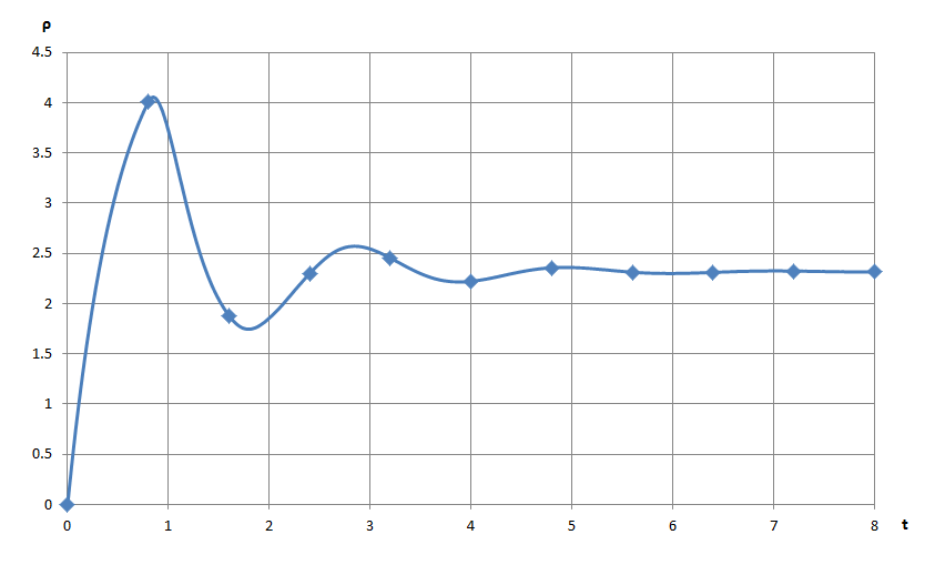
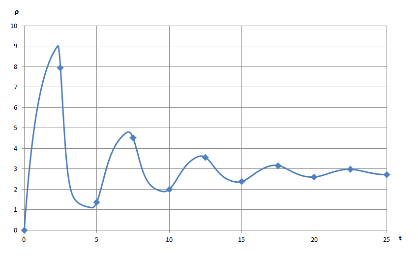
In the case when , we consider two exemplary sets of parameters (see Figure 4):
-
(vi)
,
-
(vii)
.
Computing solution in consecutive intervals requires approximating of non elementary integrals. Therefore, the recursive formula for analytical solution, even for the third interval , is computationally very demanding (as the integrals needs to be approximated independently in each iteration). Because of that, for error comparison using the analytical solution, we restrict our attention only to the interval . Approximations by numerical methods, however, are computed for the whole considered interval . Then, the initial conditions for subsequent subintervals are taken from the numerical approximations.
In order to present numerical results of (2.1) we have to introduce some additional notations. Let be a vector of points, where , , and . For given parameters of (2.1), we denote by a vector of values of exact solution of (2.1) computed in points. Let be explicit Euler, backward Euler or Runge-Kutta scheme, see [1]. For each set of parameters we tracked the behavior of the worst case error, estimated by
| (4.1) |
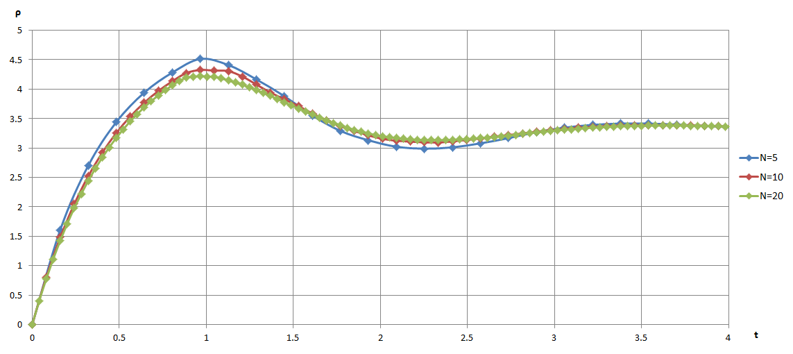
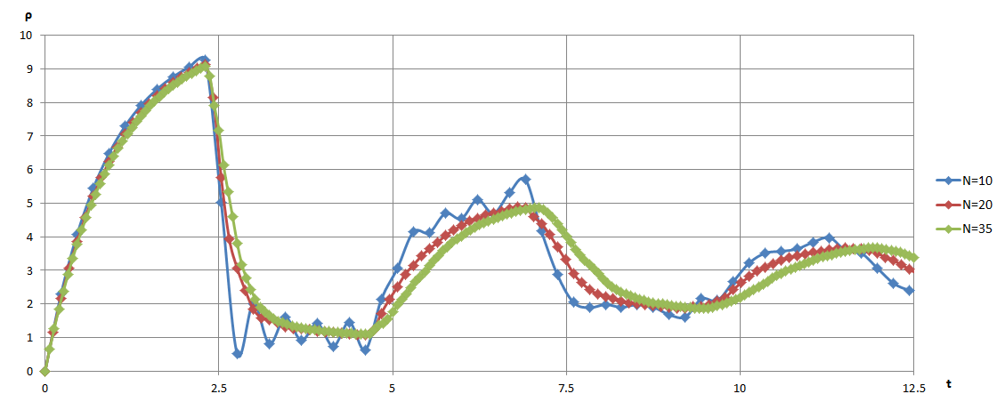
as . Results of numerical tests are presented for case (ii) in Figure 5 and Table 1, and for case (vii) in Figure 6 and Table 2, where points of consecutive iterations of the method are depicted by dots. As we can see, the case of requires more delicate analysis for choosing , because too small number leads to having points not reflecting properly the dynamics of solutions.
| explicit Euler | |||||
|---|---|---|---|---|---|
| backward Euler | |||||
| RK4 |
| explicit Euler | |||||
|---|---|---|---|---|---|
| backward Euler | |||||
| RK4 |
| explicit Euler | |||
|---|---|---|---|
| backward Euler | |||
| RK4 |
| explicit Euler | |||||
|---|---|---|---|---|---|
| backward Euler | |||||
| RK4 |
| explicit Euler | |||||
|---|---|---|---|---|---|
| backward Euler | |||||
| RK4 |
| explicit Euler | |||
|---|---|---|---|
| backward Euler | |||
| RK4 |
| explicit Euler | |||||
|---|---|---|---|---|---|
| backward Euler | |||||
| RK4 |
| explicit Euler | |||||
|---|---|---|---|---|---|
| backward Euler | |||||
| RK4 |
| explicit Euler | |||
|---|---|---|---|
| backward Euler | |||
| RK4 |
In all the cases where assumption is satisfied, viz. (i)-(iii), (vi)-(vii) we observe the theoretical convergence rate. In the cases (iv)-(v) when ratio is slightly above , some convergence to exact solutions can be observed. However, amplitude of oscillations increases with growing , leading eventually to an unstable solution (see Figure 3). Nonetheless, for a fixed number of intervals and tending with , we still can observe the theoretical convergence rate of both Euler methods and Runge-Kutta scheme (see Table 3).
4.2. Equation (1.2) with real world parameters
In previous section we proved that explicit Euler method (and its modification) gives very satisfactory results for simplified equation (2.1) and proved stability of this method. This entitles us to perform numerical simulations on more complicated equation (1.2) with both and time dependent and other parameters (time dependent as well) coming from real world processing of materials. First, let us examine solutions of (2.1) with parameters established for DP steel and copper through inverse analysis for the experimental data (uniaxial compression tests performed at constant temperatures and strain rates) using algorithm described in [20]. When equation (1.1) is used to calculate the flow stress, the results which are depicted in Figure 7, are very similar to those in Figure 1.
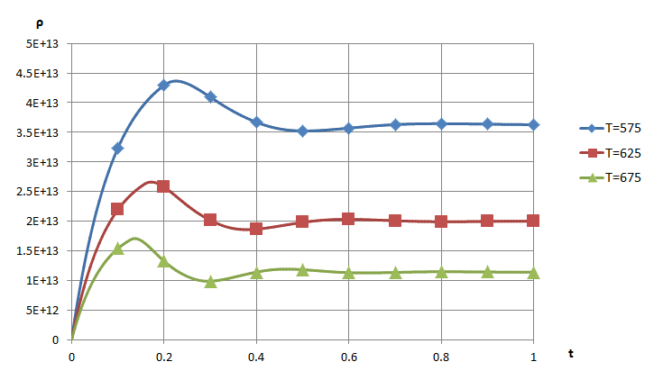
T=575°C: ,
T=625°C: ,
T=675°C: .
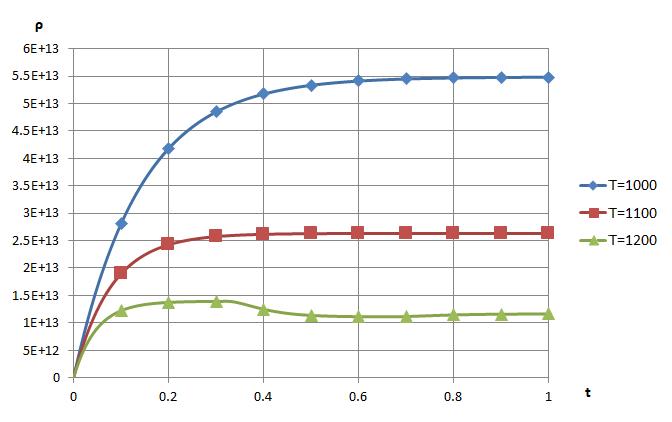
T=1000°C: ,
T=1100°C: ,
T=1200°C: .
This confirms that indeed, we are ready for modeling of real industrial process. Since it is characterized by strong heterogeneity of deformation, we decided to consider industrial process of hot strip rolling for demonstration of capabilities of the developed model. Similarly to previous laboratory case (see Figure 7), two materials, DP steel and copper, were considered. Roll pass data, which were the same for both materials, were as follows: initial thickness 20 mm, thickness reduction 50%, roll radius 400 mm and roll rotational velocity 10 rpm. Thermal-mechanical finite element (FE) model was used in the macro scale to calculate strains, stresses and temperatures. Details of the FE code are given in [12, 17]. Briefly, the Levy-Mises flow rule was used as the constitutive law:
| (4.2) |
where: , - stress and strain rate tensors, respectively, - effective strain rate, - the flow stress provided by (1.1).
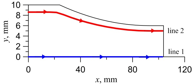
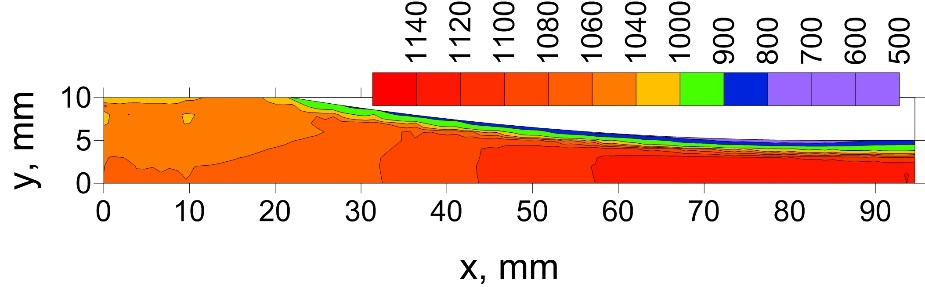
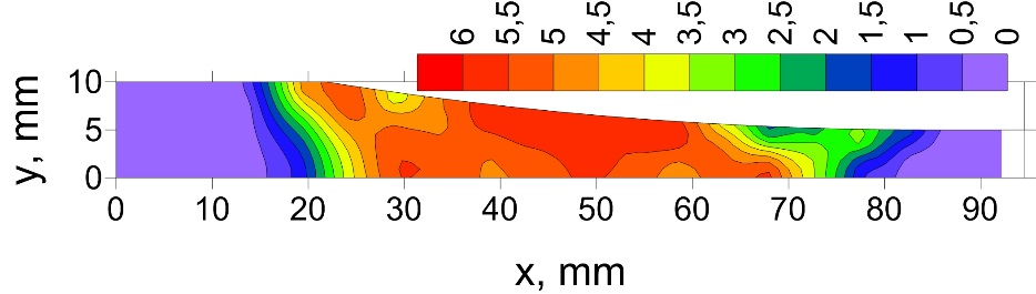
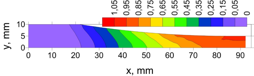
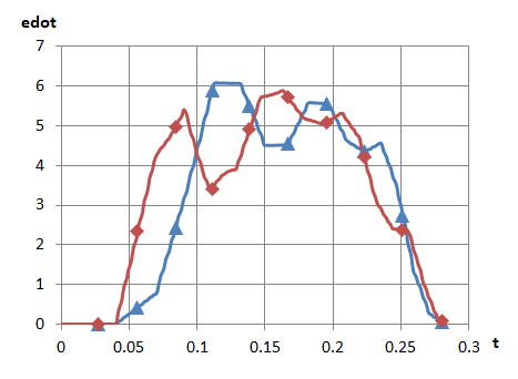
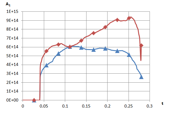
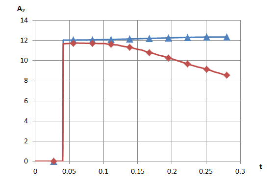
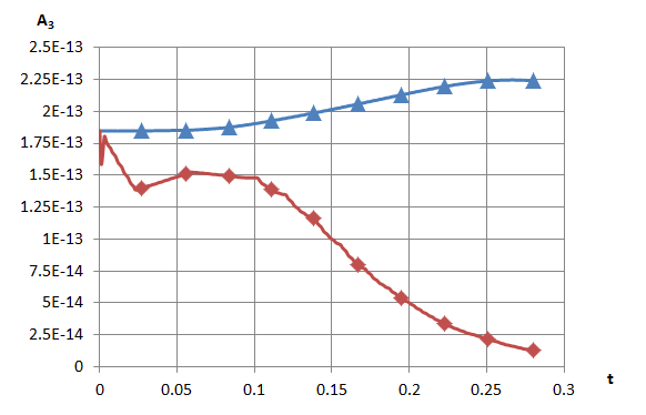
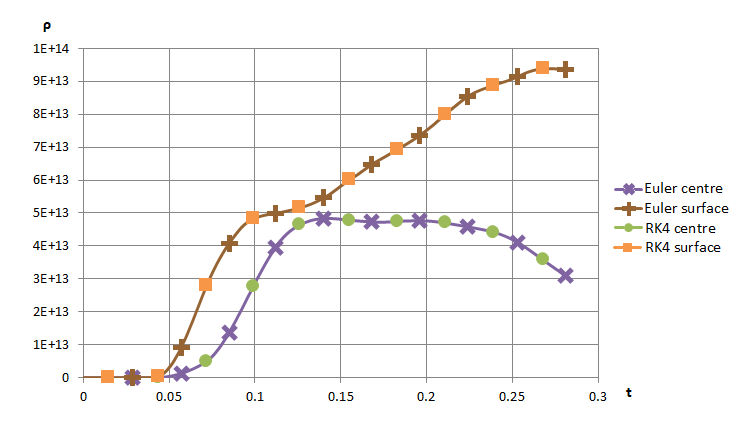
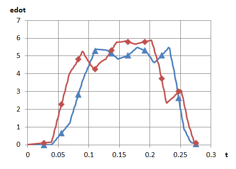
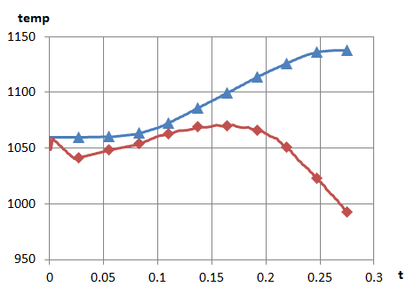
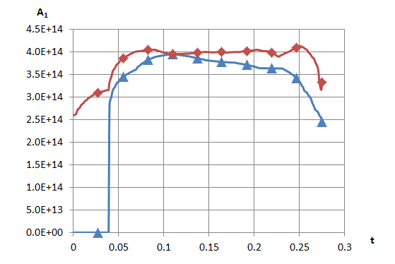
Equation (1.2) was solved along the flow lines in the deformation zone using current local values of the strain rate and the temperature. The results for two lines, one in the center of the strip and the second one close to the surface (see Figure 8), are presented on Figures 11 and 12. Let us explain the details behind these numerical experiments. Due to horizontal symmetry only a top part of the roll gap is shown in Figures 8, 9, and 10. The entry temperature was 1060°C for DP steel and 600°C for copper. Shear modulus was assumed to be time independent and equal MPa for copper and MPa for DP steel. For the assumed parameters the length of the computation domain was 105 mm and the time needed for the material point to flow through this domain was s. Finite element (FE) simulation of the rolling process was performed using FE code described in [12, 17] and calculated distributions of the temperature, strain rate and strain are shown in Figure 9 and Figure 10. Results depicted in Figure 9 are for the DP steel and in Figure 10 for the copper. On the basis of these results changes of the temperature and the strain rate along the flow lines in Figure 8 were determined, leading to time-dependent coefficients as presented on Figure 11 and Figure 12. Another important coefficient is as it is responsible for nonlinearity in (1.2). For copper it was possible to satisfactorily fit the model with , however for DP steel it had to be fractional because was not leading to satisfactory fitting. Fitting was successful with and this value was used in our simulations (cf. [12]). By the same reason, the coefficient was set to for copper and to for DP steel. The coefficient in both cases, which among other things, ensures that is never .
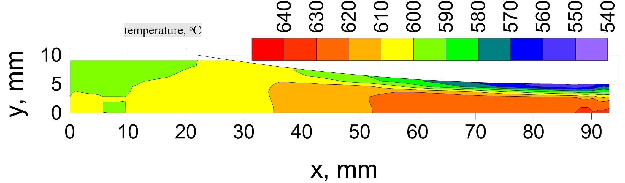
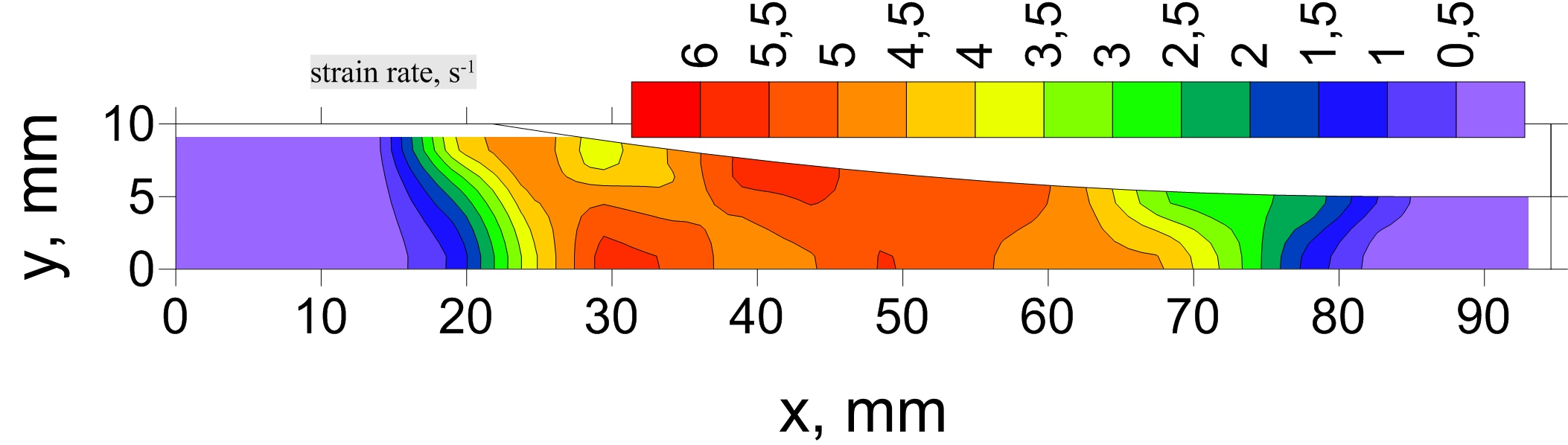
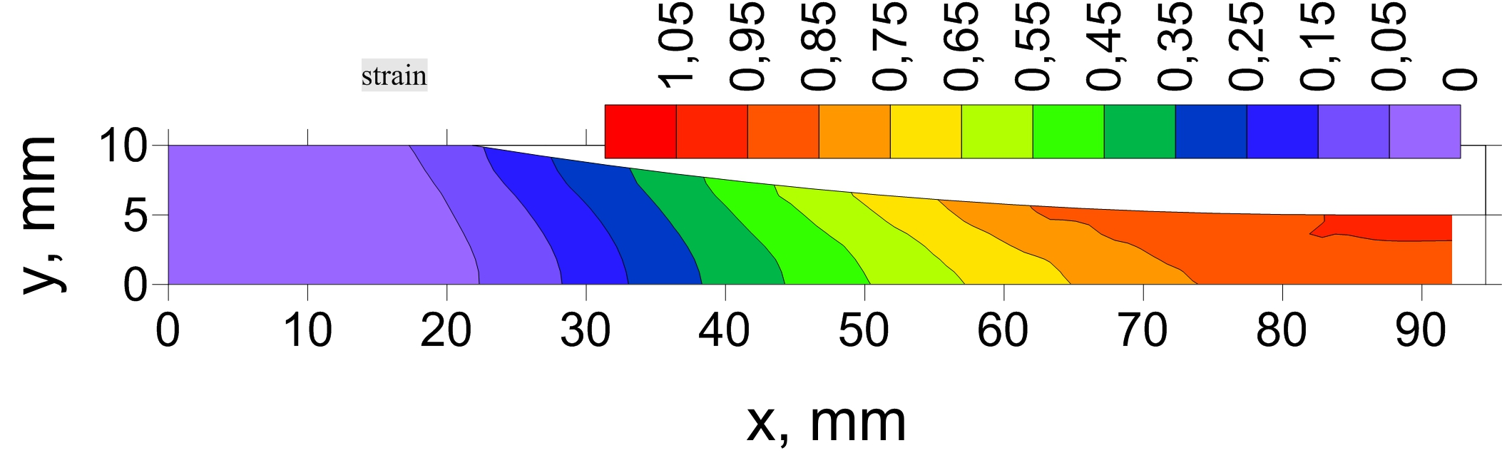
We used this data to deal with (1.2). Calculated evolution solutions with parameters evolving along the lines 1 and 2 in Figure 8 are presented in Figure 11 and Figure 12. Starting density was the same for both metals and equal . Analysis of these results shows that they react properly to distinct temperature and strain rate histories for the center and surface areas. Practical observations show that in the center the temperature increases due to deformation heating. Contrary, drop of the temperature due to heat transfer to the cool roll is observed in the surface area. As far as strain rate is considered, in the central part it decreases monotonically due to monotonic deformation of this part. The results presented in Figure 11 and Figure 12 replicate properly material behavior in these conditions of the deformation. In the surface area, where the temperature is lower and the strain rate is higher, critical dislocation density is higher and so given by equation (1.9) is reached later. In the center of the strip higher temperature leads to more dynamic recrystallization and a decrease of the dislocation density.

5. Conclusions
In the paper we have investigated mathematical aspects of evolution of dislocation density in metallic materials, modeled by delay differential equations (1.2). For typical range of real world parameters we have shown that the unique solution always exists and it is bounded. For approximation of the solution we have used the explicit Euler method. We have shown the rate of convergence of the Euler method in the case when the right-hand side function is only locally Hölder continuous. We have confirmed our theoretical findings in numerical experiments performed in special cases, when explicit solutions were known. Moreover, we have applied the algorithm to examples with real-world parameters. Despite the fact that for a Runge-Kutta method we have not been able to investigate its error under conditions , required by the equation, we tested its numerical behavior taking the Euler scheme as a benchmark. Numerical experiments showed advantage of the Runge-Kutta method over the Euler schemes. This encouraged us to use Runge-Kutta methods in real world applications. However, investigation of its theoretical properties under the assumptions are forwarded to a future work.
Acknowledgments
This research was supported by National Science Centre (Narodowe Centrum Nauki - NCN) in Poland, grant no. 2017/25/B/ST8/01823.
References
- [1] A. Bellen, M. Zennaro, Numerical methods for delay differential equations. Oxford, New York, 2003.
- [2] J. C. Butcher, Numerical methods for ordinary differential equations. Wiley, 3rd edition, Chichester, 2016.
- [3] C. H. J. Davies, private communication (data set collected from experiments). Monash University, 1994.
- [4] C. H. J. Davies, Dynamics of the evolution of dislocation populations. Scripta Metallurgica et Materialia, 30(3) (1994), 349-353.
- [5] Y. Estrin, H. Mecking, A unified phenomenological description of work hardening and creep based on one parameter models. Acta Metallurgica, 29 (1984), 57-70.
- [6] U. Foryś, M. Bodnar, J. Poleszczuk, Negativity of delayed induced oscillations in a simple linear DDE. Appl. Math. Lett. 24(6) (2011), 982-986.
- [7] L. Górniewicz, R. S. Ingarden, Mathematical Analysis for Physicists (in Polish). Wydawnictwo Naukowe UMK, 2012.
- [8] J.K. Hale, Ordinary differential equations. Second edition. Robert E. Krieger Publishing Co., Inc., Huntington, N.Y., 1980.
- [9] E. Hairer, S. P. Nørsett, G. Wanner, Solving ordinary differential equations I. Nonstiff problems. Springer, 2nd revised edition, New York, 2008.
- [10] K. Huang, R. E. Logé, A review of dynamic recrystallization phenomena in metallic materials. Materials and Design, 111 (2016), 548-574.
- [11] J. Kitowski, Ł. Rauch, M. Pietrzyk, A. Perlade, R. Jacolot, V. Diegelmann, M. Neuer, I. Gutierrez, P. Uranga, N. Isasti, G. Larzabal, R. Kuziak, U. Diekmann, Virtual strip rolling mill VirtRoll. European Commission Research Programme of the Research Fund for Coal and Steel, Technical Group TGS 4, final report from the project RFSR-CT-2013-00007, 2017.
- [12] J.G. Lenard, M. Pietrzyk, L. Cser, Mathematical and physical simulation of the properties of hot rolled products. Elsevier, Amsterdam, 1999.
- [13] S.R. Logan, The origin and status of the Arrhenius equation. Journal of Chemical Education, 59 (1982), 279-281.
- [14] H.J. McQueen, Development of dynamic recrystallization theory. Materials Science and Engineering A, 387-389 (2004), 203-208.
- [15] H. Mecking, U. F. Kocks, Kinetics of flow and strain-hardening. Acta Metallurgica, 29 (1981), 1865-1875.
- [16] P. Morkisz, P. Oprocha, P. Przybyłowicz, N. Czy˙zewska, J. Kusiak, D. Szeliga, Ł. Rauch, M. Pietrzyk, Prediction of Distribution of Microstructural Parameters in Metallic Materials Described by Differential Equations with Recrystallization Term. International Journal for Multiscale Computational Engineering, 17(3) (2019), 361-371.
- [17] M. Pietrzyk, Finite element simulation of large plastic deformation. Journal of Materials Processing Technology, 106 (2000), 223-229.
- [18] M. Pietrzyk, Ł. Madej, Ł. Rauch, D. Szeliga, Computational Materials Engineering: Achieving high accuracy and efficiency in metals processing simulations. Butterworth-Heinemann, Elsevier, Amsterdam, 2015.
- [19] H. Smith, An introduction to delay differential equations with applications to the life sciences. Texts in Applied Mathematics 57, Springer, New York, 2011.
- [20] D. Szeliga, J. Gawąd, M. Pietrzyk, Inverse analysis for identification of rheological and friction models in metal forming. Computer Methods in Applied Mechanics and Engineering, 195 (2006), 6778-6798.
- [21] J. J. Urcola, C. M. Sellars, Influence of changing strain rate on microstructure during hot deformation. Acta Metallurgica, 35 (1987), 2649-57.