Unsupervised BatchNorm Adaptation (UBNA): A Domain Adaptation Method for Semantic Segmentation Without Using Source Domain Representations

Abstract

In this paper we present a solution to the task of “unsupervised domain adaptation (UDA) of a given pre-trained semantic segmentation model without relying on any source domain representations”. Previous UDA approaches for semantic segmentation either employed simultaneous training of the model in the source and target domains, or they relied on an additional network, replaying source domain knowledge to the model during adaptation. In contrast, we present our novel Unsupervised BatchNorm Adaptation (UBNA) method, which adapts a given pre-trained model to an unseen target domain without using—beyond the existing model parameters from pre-training—any source domain representations (neither data, nor networks) and which can also be applied in an online setting or using just a few unlabeled images from the target domain in a few-shot manner. Specifically, we partially adapt the normalization layer statistics to the target domain using an exponentially decaying momentum factor, thereby mixing the statistics from both domains. By evaluation on standard UDA benchmarks for semantic segmentation we show that this is superior to a model without adaptation and to baseline approaches using statistics from the target domain only. Compared to standard UDA approaches we report a trade-off between performance and usage of source domain representations.

1 Introduction

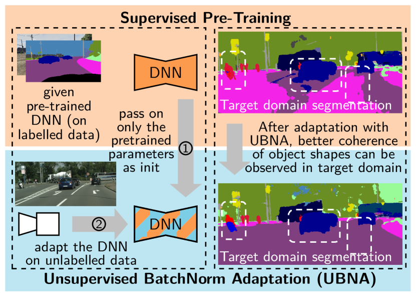
Figure 1: UBNA can be used to adapt a given pre-trained model to the target domain without using source domain representations. Target domain performance clearly improves after adaptation.

Current neural-network-based solutions to many perception tasks in computer vision rely on annotated datasets. However, the generation of these annotations, i.e., ground truth labels, is tedious and time-consuming, in particular for pixel-wise prediction tasks such as semantic segmentation [8, 48], depth estimation [14, 45, 28, 52, 51], optical flow [14, 45], or instance segmentation [40]. Due to the domain shift between datasets, neural networks usually cannot be trained in one domain (source domain) and be deployed in a different one (target domain) without a significant loss in performance [13]. For applications such as autonomous driving, virtual reality, or medical imaging, these problems are often addressed by unsupervised domain adaptation (UDA) or domain generalization (DG) approaches.

State-of-the-art approaches for UDA of semantic segmentation [25, 44, 74] usually employ annotated source domain data during adaptation. Alternatively, other approaches [30, 41] make use of an additional network to replay the source domain knowledge during the adaptation to the model. However, in practice, models are often pre-trained on non-public datasets. When adapting such a given model one might only have access to target domain data, since the source domain data cannot be passed on either for practical reasons or due to data privacy issues. In such cases, DG approaches are also inapplicable, as they have to be applied already during pre-training in the source domain. Therefore, in this work we do not aim at outperforming existing UDA or DG approaches but at solving a different very constrained task, where simultaneous access to source and target domain data is neither allowed nor required and a given model has been pre-trained in the source domain. We dub this task “UDA for semantic segmentation without using source domain representations”, i.e., a given semantic segmentation model pre-trained in the source domain is adapted to the target domain without utilizing any kind of representation from the source domain beyond the existing model parameters from pre-training.

To create a baseline method for this rather challenging task, we build on advances of UDA techniques on related image classification tasks [36, 33, 72, 78], where a few approaches exist for UDA without source domain data. However, these are either not easily transferable to semantic segmentation [33], violate our condition of not using any source domain representations [72], or apply a data-dependent evaluation protocol, where the performance on a single image is dependent on other images in the test set [36, 78]. Therefore, we propose the Unsupervised BatchNorm Adaptation (UBNA) algorithm (that can be seen as an improved version of AdaBN [36]), which adapts the statistics of the batch normalization (BN) layers to the target domain, while leaving all other model parameters untouched. In contrast to AdaBN [36], we apply a data-independent evaluation protocol after adaptation of the model. Also, we preserve some knowledge from the source domain BN statistics by not replacing these pre-trained parameters entirely with those from the target domain, instead combining them using an exponential BN momentum decay which leads to a significant boost in adaptation performance.

Our contribution with this work is threefold. Firstly, we (i) outline the task of UDA for semantic segmentation without using source domain representations. Secondly, we (ii) present Unsupervised BatchNorm Adaptation (UBNA) as a solution to this task and thereby, thirdly, (iii) enable an online-applicable UDA for semantic segmentation which we show to be operating even in a few-shot learning setup. We achieve a significant improvement over a pre-trained semantic segmentation model without adaptation and we also outperform respective baseline approaches making use of adapting the normalization layers, which we transferred to a comparable setting for semantic segmentation.

2 Related Work

In this section we first discuss UDA and DG approaches for semantic segmentation. Afterwards, we discuss UDA approaches not relying on source domain data, and UDA approaches relying on the use of normalization layers.

UDA with Source Domain Representations: Approaches to UDA can be divided into three main categories. Firstly, style transfer approaches [16, 18, 38, 75], where the source domain images get altered to match the style of the target domain. Secondly, domain-adversarial training [3, 5, 9, 11, 19, 20, 65, 67, 73], where a discriminator network is employed to enforce a domain-invariant feature extraction. Thirdly self-training, where pseudo-labels are generated for the target domain samples, which are then used as additional training material [6, 38, 44, 61, 80]. Often methods from all three categories are combined to achieve state-of-the-art results [25, 64, 70, 74, 75, 79]. On the other hand, the approaches of [2, 30, 41, 62, 63, 72] use auxiliary information (e.g., an auxiliary network) from the source domain during adaptation. While this removes the need for source data during adaptation, it imposes the need of additional information about the source domain, which still is a kind of source domain representation. In contrast, we propose an adaptation only relying on a few adaptation steps on few unlabelled target domain data, thereby solving a more constrained task in an efficient fashion.

Domain Generalization: Approaches for DG [10, 32, 58, 77] aim at an improvement in the target domain without having access to target domain data. Only few works exist for semantic segmentation [7, 77]. In contrast to DG, we assume the source data to be unavailable. Accordingly, we consider DG methods rather applicable during pre-training but not during adaptation of a given model and without access to source data, which we require in our task definition.

UDA w/o Source Domain Representations: Improving the performance of a given model in the target domain without using source domain representations during adaptation is challenging and so far rarely addressed. Most techniques rely on training with pseudo-labels in the target domain, generated by the model pre-trained in the source domain [35, 76]. Additionally, alignment methods for the latent space distribution [34, 39, 76] can be applied. Other approaches apply selection methods for “good” pseudo labels [35]. In a recent approach, Li et al. [33] propose to train a class-conditional generator producing target-style data examples. Collaboration of this generator with the prediction model is shown to improve performance in the target domain without the use of source data. So far the mentioned frameworks are formulated only for image classification or object detection, while we address semantic segmentation. Also, our proposed adaptation method is potentially real-time capable and easier to generalize to other tasks as it requires only a few update steps of the BN statistics parameters and does thereby not rely on gradient optimization.

UDA via Normalization Layers: Normalization techniques [1, 21, 22, 23, 46, 47, 66, 59, 71] are commonly used in many network architectures. For UDA often new domain-adaptation-specific normalization layers [4, 42, 43, 54, 69] are proposed, e.g., Chang et al. [4] propose to use domain-specific BN statistics but share all other network parameters. Also, the approach of Xu et al. [73] combines adversarial learning with a BN statistics re-estimation in the target domain. In contrast to our method, these approaches all require training on labeled source data during adaptation.

Other recent works from Li et al. [36, 37] and Zhang et al. [78] show that BN statistics can be re-estimated in the target domain on the entire test set or over batches thereof for performance improvements which also can be seen as a kind of UDA without source domain representations. However, both approaches determine the BN statistics during inference in dependency of all test data, making the performance on one sample depend on (the availability of) the other samples present in the test set or batch. On the other hand, we use a separate adaptation set, removing the inter-image dependency at test time. Also, our UBNA method shows that it is beneficial not to use statistics solely from the target domain (as in [36, 37, 78]), but to mix source with target statistics by using an exponentially decaying BN momentum factor. Concurrently, Schneider et al. [57] found similar improvements by mixing statistics from perturbed and clean images for adversarial robustness, which we feel supports our novel finding on the defined UDA task.

3 Revisiting Batch Normalization, Notations

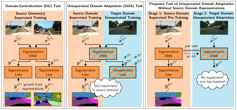
Figure 2: Different task setups to improve performance on unseen data for semantic segmentation: In domain generalization (left) the aim is to generalize to unseen data using diverse source domain data $\mathcal{D}^{\mathrm{S}_{1}}$, $\mathcal{D}^{\mathrm{S}_{2}}$. Meanwhile, in unsupervised domain adaptation (center), the model is trained simultaneously on the source domain $\mathcal{D}^{\mathrm{S}}$ and on the target domain $\mathcal{D}^{\mathrm{T}}$, while still using supervision from the source domain during the adaptation. In contrast, we propose a two-stage approach (right): A given semantic segmentation has been pre-trained in the source domain $\mathcal{D}^{\mathrm{S}}$, and in a second stage it is afterwards adapted to the target domain $\mathcal{D}^{\mathrm{T}}$ in an unsupervised fashion.

Before we will introduce our UBNA method in Section 4, in this section we briefly revisit the batch normalization (BN) layer and thereby introduce necessary notations. Following the initial formulation from [23], we consider a batch of input feature maps $\bm{f}_{\ell}\in\mathbb{R}^{B\times H_{\ell}\times W_{\ell}\times C_{\ell}}$ for the BN layer $\ell$ with batch size $B$, height $H_{\ell}$, width $W_{\ell}$, and number of channels $C_{\ell}$. In a convolutional neural network (CNN) each feature $f_{\ell,b,i,c}\in\mathbb{R}$ with batch-internal sample index $b\in\mathcal{B}=\left\{1,...,B\right\}$, spatial index $i\in\mathcal{I}_{\ell}=\left\{1,...,H_{\ell}\cdot W_{\ell}\right\}$, and channel index $c\in\mathcal{C}_{\ell}=\left\{1,...,C_{\ell}\right\}$ is batch-normalized according to

$$\hat{f}_{\ell,b,i,c}=\gamma_{\ell,c}\cdot\left(f_{\ell,b,i,c}-\mu_{\ell,c}\right)\cdot\left(\sigma_{\ell,c}^{2}+\epsilon\right)^{-\frac{1}{2}}+\beta_{\ell,c}\;.$$ (1)

Here, $\bm{\gamma}_{\ell}=(\gamma_{\ell,c})\in\mathbb{R}^{C_{\ell}}$ and $\bm{\beta}_{\ell}=(\beta_{\ell,c})\in\mathbb{R}^{C_{\ell}}$ are learnable scaling and shifting parameters, respectively, $\epsilon\in\mathbb{R}$ is a small number, and $\bm{\mu}_{\ell}=(\mu_{\ell,c})\in\mathbb{R}^{C_{\ell}}$ and $\bm{\sigma}_{\ell}=(\sigma_{\ell,c})\in\mathbb{R}^{C_{\ell}}$ are the computed mean and standard deviation, respectively, over the batch samples $b\in\mathcal{B}$ in layer $\ell$ and feature map $c$. Note that in a CNN the statistics are also calculated over the invariant spatial dimension $i$.

At each training step $k$ a batch $\mathcal{B}$ is taken from the set of training samples. Then, mean $\hat{\bm{\mu}}^{(k)}_{\ell}$ and standard deviation $\hat{\bm{\sigma}}^{(k)}_{\ell}$ of the features in the current batch $\mathcal{B}$ are computed as

$$\hat{\mu}^{(k)}_{\ell,c} =\frac{1}{BH_{\ell}W_{\ell}}\sum_{b\in\mathcal{B}}\sum_{i\in\mathcal{I}}f_{\ell,b,i,c},$$ (2)

$$\left(\hat{\sigma}^{(k)}_{\ell,c}\right)^{2} =\frac{1}{BH_{\ell}W_{\ell}}\sum_{b\in\mathcal{B}}\sum_{i\in\mathcal{I}}\left(f_{\ell,b,i,c}-\hat{\mu}^{(k)}_{\ell,c}\right)^{2}.$$ (3)

During training, the values from (2) and (3) are directly used in (1), meaning $\bm{\mu}_{\ell}=\hat{\bm{\mu}}^{(k)}_{\ell}$ and $\bm{\sigma}_{\ell}=\hat{\bm{\sigma}}^{(k)}_{\ell}$. As preparation for inference, however, mean and variance over the training dataset are tracked progressively using (2) and (3) as

$$\check{\mu}_{\ell,c}^{(k)} =\left(1-\eta\right)\cdot\check{\mu}_{\ell,c}^{(k-1)}+\eta\cdot\hat{\mu}_{\ell,c}^{(k)},$$ (4)

$$\left(\check{\sigma}_{\ell,c}^{(k)}\right)^{2} =\left(1-\eta\right)\cdot\left(\check{\sigma}_{\ell,c}^{(k-1)}\right)^{2}+\eta\cdot\left(\hat{\sigma}_{\ell,c}^{(k)}\right)^{2},$$ (5)

where $\eta\in\left[0,1\right]$ is a momentum parameter. After training for $K$ steps, the final values from (4) and (5) are used for inference, i.e., $\bm{\mu}_{\ell}=\check{\bm{\mu}}^{(K)}_{\ell}$ and $\bm{\sigma}_{\ell}=\check{\bm{\sigma}}^{(K)}_{\ell}$ for the normalization in (1). Note that updating only the BN statistics parameters is computationally not very expensive, as no gradients have to be backpropagated through the network.

4 Task and Method

Here, we define the task of “unsupervised domain adaptation for semantic segmentation without using source domain representations”, and describe how we solve it by our Unsupervised BatchNorm Adaptation (UBNA) method.

4.1 UDA w/o Source Domain Representations

The aim of our task is to improve performance of a semantic segmentation model, trained in a source domain $\mathcal{D}^{\mathrm{S}}$, on a target domain $\mathcal{D}^{\mathrm{T}}$. As shown in Fig. 2 on the right hand side in contrast to previous task definitions (left and middle parts), we introduce a two-stage approach consisting of a supervised pre-training stage and an unsupervised adaptation stage.

Stage 1—Supervised Pre-Training: In the first stage, the model is trained using image-label pairs $(\bm{x}^{\mathcal{D}^{\mathrm{S}}},\overline{\bm{y}}^{\mathcal{D}^{\mathrm{S}}})$ from the source domain $\mathcal{D}^{\mathrm{S}}$, yielding the model’s output $\bm{y}^{\mathcal{D}^{\mathrm{S}}}$. The model is optimized in a supervised fashion using an arbitrary loss between the model’s output $\bm{y}^{\mathcal{D}^{\mathrm{S}}}$ and the ground truth $\overline{\bm{y}}^{\mathcal{D}^{\mathrm{S}}}$. DG methods could also be applied in this stage. After pre-training is finished, the model parameters are passed on to the second stage, the adaptation stage. In particular, neither further explicit information, such as data or labels is passed on, nor any implicit information about the source domain, such as a generator networks.

Stage 2—Unsupervised Domain Adaptation: In the second stage only image samples $\bm{x}^{\mathcal{D}^{\mathrm{T}}}$ from the target domain $\mathcal{D}^{\mathrm{T}}$ are allowed to be used for adaptation of a given pre-trained model, either through some update rule for the pre-trained weights or some unsupervised loss function. Due to the catastrophic forgetting problem in neural networks, this presents a difficult task, as the semantic segmentation performance could be expected to decrease, if the model parameters are changed without keeping the supervision for the semantic segmentation [24, 27].

Discussion: Following, we analyze this task in terms of (1) applicability, (2) online capability, and (3) comparability w.r.t. the known tasks of domain generalization (DG) and unsupervised domain adaptation (UDA), as shown in Fig. 2.

Our task is applicable to a given pre-trained model, whenever one has access to target data. This is in contrast to UDA methods requiring simultaneous access to both source and target data (cannot always be granted due to data privacy issues). DG methods on the other hand require access to source data and are therefore applied during pre-training, which is something we consider “out of our hands” for the scope of our adaptation task. This also means that if a model has already been pre-trained and the source data is not available, DG methods cannot be applied, while methods solving our task are still applicable.

Regarding online capability, our task provides the general possibility of online adaptation of a model, whereas solutions to DG as of their definition are offline methods applied in pre-training. UDA, on the other hand, relies on the source data and labels, the model was initially trained on, which also limits their online capability, as usually the source data cannot be stored on the target device.

Regarding comparability, a fair comparison and conclusive analysis w.r.t. DG methods is hardly possible as they use additional source data (cf. Fig. 2), while solutions to our task use additional target data (the latter being available during inference/adaptation!). Therefore, experimental comparison to DG cannot be provided, due to the strong dependence on the chosen additional pre-training/adaptation data. We can, however, compare to UDA techniques using the same pre-training/adaptation data as required by our task. Such methods are of course expected to outperform solutions to our task due to the additional use of labelled source data during adaptation.

4.2 UBNA Learning Approach

Our UBNA approach implements the adaptation (second stage) of our task definition in Fig. 2 (right side) and therefore assumes a pre-trained semantic segmentation model, which is supposed to be adapted to the target domain $\mathcal{D}^{\mathrm{T}}$. Also, our approach assumes that the network contains batch normalization (BN) layers, which were trained as described in Sec. 3. During our UBNA approach, all learnable parameters are kept constant, only the statistics $\bm{\mu}_{\ell}$ and $\bm{\sigma}_{\ell}$ of the BN layers $\ell$ are adapted.

Offline Protocol: For the second (the adaptation) stage, we initialize all statistics parameters using (4) and (5) as

$$\bm{\mu}_{\ell}^{(\kappa=0)}=\check{\bm{\mu}}_{\ell}^{(K)},\bm{\sigma}_{\ell}^{(\kappa=0)}=\check{\bm{\sigma}}_{\ell}^{(K)},$$ (6)

with $K$ being the last step of the pre-training stage. Modifying the running mean and variance updates from (4) and (5), respectively, by a batch-dependent momentum factor $\eta^{(\kappa)}$, we update all BN statistics in each adaptation step $\kappa$ as

$$\mu_{\ell,c}^{(\kappa)} =\left(1\!-\!\eta^{(\kappa)}\right)\cdot\mu_{\ell,c}^{(\kappa-1)}+\eta^{(\kappa)}\cdot\hat{\mu}_{\ell,c}^{(\kappa)},$$ (7)

$$\left(\sigma_{\ell,c}^{(\kappa)}\right)^{2}\!\!\! =\left(1\!-\!\eta^{(\kappa)}\right)\cdot\left(\sigma_{\ell,c}^{(\kappa-1)}\right)^{2}\!\!+\eta^{(\kappa)}\cdot\left(\hat{\sigma}_{\ell,c}^{(\kappa)}\right)^{2}\!\!\!,$$ (8)

with each batch $\mathcal{B}$ being sampled randomly from the target domain. The batch-dependent momentum factor $\eta^{(\kappa)}$ is supposed to achieve a compromise between two conflicting goals: On the one hand, we want to adapt the BN statistics to the target domain. On the other hand, the initial statistics were optimized to the weights performing a task in the source domain, which is why the mismatch between statistics parameters and network weights should not become too large. Conclusively, we choose a decay protocol

$$\eta^{(\kappa)}=\eta^{(0)}\exp\left(-\kappa\cdot\alpha^{\mathrm{BATCH}}\right),$$ (9)

determined by a batch-wise decay factor $\alpha^{\mathrm{BATCH}}$, which adapts the statistics to the target domain in a progressively decaying amount, while still keeping the task-specific knowledge learned in the source domain. When using a decay factor of $\alpha^{\mathrm{BATCH}}>0$, we dub our method UBNA, and if using $\alpha^{\mathrm{BATCH}}=0$ (no decay), we dub it UBNA⁰.

Online Protocol: Introducing a constraint into our offline protocol, we can derive an online-capable version of our approach. Here, we impose that the batches contain temporally ordered images, such that the adaptation step index $\kappa$ is equal to a time index $t\;\left[\mathrm{sec}\right]$ up to a scale factor. Assuming a batch size $B$ and a frame rate $\frac{1}{\Delta t}\;\left[\mathrm{frames/sec}\right]$, this constraint can be defined as $\frac{t}{\Delta t\cdot B}=\kappa\in\mathbb{N}$.

Layer-Wise Weighting: Previous approaches (e.g., [49]) indicate that the domain mismatch occurs more strongly in the initial layers. This can be considered by weighting the batch-dependent momentum factor $\eta^{(\kappa)}$ in (9) differently for each BN layer $\ell\in\left\{1,..,L\right\}$, with the total number of BN layers $L$, as

$$\eta_{\ell}^{(\kappa)}\!\!=\!\eta^{(\kappa)}\exp\!\left(-\ell\cdot\alpha^{\mathrm{LAYER}}\right).$$ (10)

The weighting is determined through the factor $\alpha^{\mathrm{LAYER}}$.

If $\alpha^{\mathrm{LAYER}},\alpha^{\mathrm{BATCH}}>0$, we dub our method UBNA⁺, meaning that the statistics parameters in the initial layers are adapted more rapidly than in the later layers. This also follows the idea to further improve the trade-off between adapting to the target domain (with the initial layers) and keeping the task-specific knowledge learned during pre-training in the source domain (in the later layers).

5 Implementation Details

Following, we describe the experimental details of our framework which is implemented in PyTorch [50].

Table 1: Number of used images in the databases for pre-training (source domain $\mathcal{D}^{\mathrm{S}}$) and adaptation (target domain $\mathcal{D}^{\mathrm{T}}$).

Dataset	Domain	train	validate	test
		or adapt
​ GTA-5 [53]	$\mathcal{D}^{\mathrm{S}}$	24,966	-	-
SYNTHIA [55]	$\mathcal{D}^{\mathrm{S}}$	9,400	-	-
Cityscapes [8]	$\mathcal{D}^{\mathrm{S}}$	2,975	-	-
​ Cityscapes [8]	$\mathcal{D}^{\mathrm{T}}$	89,250	500	1,525
KITTI [14, 45]	$\mathcal{D}^{\mathrm{T}}$	29,000	200	200

Datasets: To pre-train the semantic segmentation models we use the synthetic datasets GTA-5 [53] and SYNTHIA [55], as well as the real dataset Cityscapes [8] as source domains $\mathcal{D}^{\mathrm{S}}$ as defined in Tab. 1. For adaptation, we use the training splits of Cityscapes and KITTI as target domains $\mathcal{D}^{\mathrm{T}}$. We evaluate on the respective validation sets.

Network Architecture: We use an encoder-decoder architecture with skip connections as in [15, 29], where we modify the last layer to have $19$ feature maps, which are converted to pixel-wise class probabilities using a softmax function. For comparability to previous works [25, 70, 75], the encoder is based on the commonly used ResNet [17] and VGG-16 [60] architectures, (pre-)pre-trained on ImageNet [56]. If not mentioned otherwise, we use VGG-16.

Training Details: For pre-training, we resize all images to a resolution of $1024\times 576$, $1024\times 608$, and $1024\times 512$ for images from GTA-5, SYNTHIA, and Cityscapes, respectively. Afterwards, we randomly crop to a resolution of $640\times 192$. We apply horizontal flipping, random brightness ($\pm 0.2$), contrast ($\pm 0.2$), saturation ($\pm 0.2$) and hue ($\pm 0.1$) transformations as input augmentations. We pre-train our segmentation models for $20$ epochs (1 epoch corresponds to approximately $10,000$ training steps) with the ADAM optimizer [26], a batch size of $12$, and a learning rate of $10^{-4}$, which is reduced to $10^{-5}$ after $15$ epochs. For adaptation we use resolutions of $1024\times 512$ and $1024\times 320$ for Cityscapes and KITTI, respectively. Here, we use a batch size of $6$ but only adapt for $50$ steps. Our first setting introduces a constant momentum factor $\eta^{(0)}\!=\!0.1$, which we dub UBNA⁰ ($\eta^{(0)}\!=\!0.1$, $\alpha^{\mathrm{BATCH}}\!=\!\alpha^{\mathrm{LAYER}}\!=\!0$). For our UBNA model we use a batch-wise decay factor of $\alpha^{\mathrm{BATCH}}\!=\!0.08$ ($\eta^{(0)}\!=\!0.1$, $\alpha^{\mathrm{BATCH}}\!=\!0.08$, $\alpha^{\mathrm{LAYER}}\!=\!0$). Additionally, we apply the layer-wise weighting of our UBNA⁺ method, which, however, requires target-domain-specific tuning of hyperparameters: $\eta^{(0)}\!=\!0.1$, $\alpha^{\mathrm{BATCH}}\!=\!0.08$, $\alpha^{\mathrm{LAYER}}\!=\!0.03$ when adapting to Cityscapes, and $\eta^{(0)}\!=\!0.1$, $\alpha^{\mathrm{BATCH}}\!=\!0.08$, $\alpha^{\mathrm{LAYER}}\!=\!0.3$ when adapting to KITTI. As common for UDA methods, we determined optimal hyperparameters on target domain validation sets. An analysis is given in the supplementary.

Evaluation Metrics: The semantic segmentation is evaluated using the mean intersection over union (mIoU) [12], which is computed considering the classes defined in [8]. We evaluate over all 19 defined classes, except for models, which have been pre-trained on SYNTHIA. Here, we follow [31, 68] and evaluate over subsets of 13 and 16 classes. We also evaluate the per-class intersection over union (IoU).

6 Experimental Evaluation

To evaluate our method, we start by comparing our approach to other approaches that make use of adapting the BN layers, and to standard UDA approaches using source data supervision during adaptation. Afterwards, we show the online and few-shot capability of UBNA and an extensive ablation study over different network architectures.

6.1 Comparison to Normalization Approaches

Table 2: Comparison to normalization approaches: Performance on the Cityscapes validation set for the adaptation from SYNTHIA ($\mathcal{D}^{\mathrm{S}}$, third column) or GTA-5 ($\mathcal{D}^{\mathrm{S}}$, fourth column) to Cityscapes ($\mathcal{D}^{\mathrm{T}}$) in comparison to other normalization approaches (batch size $B=6$). The methods from [36] and [78] have been reimplemented by us for comparability.

Method	Source data during [-0.07cm] adaptation	$\mathcal{D}^{\mathrm{S}}$: SYNTHIA mIoU (%) (16 classes)	$\mathcal{D}^{\mathrm{S}}$: GTA-5 mIoU (%) (19 classes)
No adaptation	-	30.0	31.5
Li et al. [36]	no	31.2	34.7
Zhang et al. [78]	no	31.5	34.6
UBNA0	no	32.6	33.9
UBNA	no	34.4	36.1
UBNA+	no	34.6	36.5

While for semantic segmentation no baseline approaches exist that we could report on our task, we still want to facilitate a comparison. Therefore, we reimplemented the approaches of Li et al. (AdaBN, [36]), who effectively recalculate the statistics of the BN layers on the target domain, and Zhang et al. [78], who evaluate using the statistics from just a single batch of images during testing. Due to fairness for AdaBN, [36] we also used the adaptation dataset to determine the target domain statistics, while for Zhang et al. [78] this was not possible due to the batch-wise normalization. As can be seen in Tab. 2 and Fig. 3, both baseline approaches are able to improve the model performance in the target domain. On the other hand, a simple experiment with constant BN momentum (UBNA⁰) in Fig. 3 shows that after a few batches there is a maximum in performance, which is a typical behaviour we observed on all considered datasets (cf. supplementary material). UBNA⁰ exceeds baseline performance on the SYNTHIA to Cityscapes but not on the GTA-5 to Cityscapes adaptation, yet indicating that it is beneficial not to discard the source domain statistics entirely. As UBNA⁰ does not show stable convergence, we propose our UBNA and UBNA⁺ methods both achieving a stable convergence to some maximum performance after $\kappa=50$ steps by using a decaying BN momentum factor as described in (9). Interestingly, the hyperparameter $\alpha^{\mathrm{BATCH}}=0.08$ can be determined independently of the used dataset combination which shows the general applicability of UBNA. We outperform all baseline approaches on all used dataset combinations as can be seen in Tab. 2.

[width=1.0]figs/baseline_comparison/baseline_comparison_synthia_to_cs

Figure 3: Comparison to normalization approaches: Performance on the Cityscapes validation set for the adaptation from SYNTHIA ($\mathcal{D}^{\mathrm{S}}$) to Cityscapes ($\mathcal{D}^{\mathrm{T}}$) in dependence of the adaptation step $\kappa$ (batch size $B=6$). We also show results when using the statistics from the source domain (no adaptation) and from the target domain (AdaBN by Li et al. [36]).

6.2 Comparison to UDA Approaches

Table 3: Comparison to UDA: Performance of UBNA and UBNA⁺ (right task, Fig. 2) in comparison to UDA methods (center task, Fig. 2) on the Cityscapes validation set for the adaptation from GTA-5 ($\mathcal{D}^{\mathrm{S}}$) to Cityscapes ($\mathcal{D}^{\mathrm{T}}$) (upper part) and SYNTHIA ($\mathcal{D}^{\mathrm{S}}$) to Cityscapes ($\mathcal{D}^{\mathrm{T}}$) (lower part). We evaluate VGG-16-based models, compare different methods (second column, values from the respective papers), show if they use labeled source data during UDA (third column), evaluate the class-wise IoU performance (%), and give an mIoU (%) over 19 classes. For SYNTHIA we evaluate over 16 classes (excluding classes marked with $*$) and over 13 classes (excluding classes marked with $**$) as is common in the field [31, 67]. Best results for UDA with and w/o source data, respectively, are printed in boldface.

Source data	Method	Source data during [-0.07cm] adaptation	road	sidewalk	building	wall∗∗	fence∗∗	pole∗∗	traffic light	traffic sign	vegetation	terrain∗	sky	person	rider	car	truck∗	bus	on rails∗	motorbike	bike	$\mathrm{mIoU}$ (%) (19 classes)
GTA-5	Vu et al. [67]	yes	86.9	28.7	78.7	28.5	25.2	17.1	20.3	10.9	80.0	26.4	70.2	47.1	8.4	81.5	26.0	17.2	18.9	11.7	1.6	36.1
	Dong et al. [9]	yes	89.8	46.1	75.2	30.1	27.9	15.0	20.4	18.9	82.6	39.1	77.6	47.8	17.4	76.2	28.5	33.4	0.5	29.4	30.8	41.4
	Yang et al. [74]	yes	90.1	41.2	82.2	30.3	21.3	18.3	33.5	23.0	84.1	37.5	81.4	54.2	24.3	83.0	27.6	32.0	8.1	29.7	26.9	43.6
	No adaptation	-	55.8	21.9	65.9	15.2	14.7	27.5	31.0	17.9	77.8	19.5	74.4	55.2	12.1	71.7	11.9	3.3	0.5	13.2	9.6	31.5
	UBNA	no	80.8	29.4	77.6	19.8	17.1	33.9	29.3	20.5	73.9	16.8	76.7	58.3	15.2	79.1	13.6	12.5	5.7	14.1	10.8	36.1
	UBNA+	no	79.9	29.9	78.1	21.1	16.5	33.8	29.7	20.6	75.6	18.4	78.0	58.4	14.6	79.4	14.8	13.0	5.8	14.6	10.6	36.5
																						16 cl.	13 cl.
SYNTHIA	Lee et al. [31]	yes	71.1	29.8	71.4	3.7	0.3	33.2	6.4	15.6	81.2	-	78.9	52.7	13.1	75.9	-	25.5	-	10.0	20.5	36.8	42.4
	Dong et al. [9]	yes	70.9	30.5	77.8	9.0	0.6	27.3	8.8	12.9	74.8	-	81.1	43.0	25.1	73.4	-	34.5	-	19.5	38.2	39.2	-
	Yang et al. [74]	yes	73.7	29.6	77.6	1.0	0.4	26.0	14.7	26.6	80.6	-	81.8	57.2	24.5	76.1	-	27.6	-	13.6	46.6	41.1	-
	No adaptation	-	49.4	20.8	61.5	3.6	0.1	30.5	13.6	14.1	74.4	-	75.5	53.5	10.6	47.2	-	4.8	-	3.0	17.1	30.0	35.2
	UBNA	no	72.3	26.6	73.0	2.3	0.3	31.5	12.1	16.6	72.1	-	75.6	45.4	13.6	61.2	-	8.5	-	8.5	30.1	34.4	40.7
	UBNA+	no	71.5	27.3	72.9	2.5	0.3	32.0	12.7	16.7	74.6	-	75.4	47.1	13.6	61.4	-	8.5	-	8.3	29.2	34.6	41.0

Another type of comparison can be drawn to standard UDA approaches, which we present for the widely accepted standard benchmarks GTA-5 to Cityscapes and SYNTHIA to Cityscapes in Table 3. We would like to emphasize here that the white and gray parts in these tables are not completely comparable, as standard UDA approaches (white parts) make use of source data (cf. middle task in Fig. 2) during the adaptation, while our approach does not make use of this supervision (cf. right task in Fig. 2). Still, some conclusions can be drawn: Firstly, the improvement and final performance of our model is not as high as for standard UDA approaches, which is to be expected due to our much more constrained task of an adaptation without source data, where UDA approaches are not even applicable. Secondly, Tab. 3 shows that we improve the baselines without adaptation by $5.0\%$ and $4.6\%/5.8\%$ absolute on the two adaptations from GTA-5 to Cityscapes and SYNTHIA to Cityscapes, respectively. Moreover, our UBNA⁺ model improves the baseline in the respective single classes in 16 out of 19 and 12 out of 16 cases in terms of IoU, which shows a pretty consistent improvement for the majority of classes. Accordingly, our method still significantly improves a baseline trained without any adaptation. For a more detailed qualitative discussion, we refer to the supplementary. In conclusion, these observations show a trade-off between final performance and usage of labelled source data during adaptation compared to UDA approaches.

6.3 Few-Shot Capability

Table 4: Few-shot adaptation: Performance of UBNA⁺ on the Cityscapes validation set for the adaptation from SYNTHIA ($\mathcal{D}^{\mathrm{S}}$, top row) or GTA-5 ($\mathcal{D}^{\mathrm{S}}$, bottom row) to Cityscapes ($\mathcal{D}^{\mathrm{T}}$) for different numbers of total images used for adaptation (average over 10 different experiments). Results after the $50$th adaptation step, where in a single experiment the same batch is used in all adaptation steps, showing the few-shot capability of our approach.

# of images $B$ per batch	-	1	2	3	5	10
mIoU (%) (16 classes)	30.0	33.1	33.3	34.2	34.3	34.3
mIoU (%) (19 classes)	31.0	34.9	35.6	36.3	35.9	36.2

To investigate how many target domain images are necessary for a successful adaptation, we use only a single image batch for $50$ steps of adaptation and thereby show that our method is indeed few-shot capable. For these experiments we chose the best performing method UBNA⁺. In Tab. 4 we show results for a network adapted with only $B=1$, $2$, $3$, $5$, or $10$ images in the batch. As we suspected that the choice of images might have a significant impact on the final result, the results in Tab. 4 are averaged over 10 different experiments. Here, on average, we can observe performance improvements even for the adaptation with a single image (see supplementary for more detailed results). Indeed, one can observe a significant and consistent improvement in any of the 10 experiments with an average improvement from $3\%$ to about $5\%$ absolute, which shows our method’s few-shot capability.

6.4 Online (i.e., Video Adaptation) Capability

As our method does not require the source dataset to be available during adaptation, we are able to adapt the segmentation network in an online setting using sequential images from a video. As our target domain adaptation data we use the video from Stuttgart (images in sequential order), which is provided as part of the Cityscapes dataset [8]. Tab. 5 gives UBNA⁺ results when using different numbers of sequential images per batch, meaning that the total number of sequential images is proportional to the batch size, while we adapt for 50 steps in all experiments. We observe that in all experiments we can improve the baseline by about $3\%$ to $4\%$ absolute. Also, using the VGG-16 backbone, inference of the segmentation network with or without UBNA is realtime-capable with $23\text{\,}\mathrm{f}\mathrm{p}\mathrm{s}$ on an NVIDIA GeForce GTX 1080 Ti graphics card, since the computational effort to update of the BN statistics using (7) and (8) is negligible. The frame rate of Cityscapes is about $16.66\text{\,}\mathrm{f}\mathrm{p}\mathrm{s}$, accordingly a UBNA model utilizing a VGG-16 backbone would be real time-capable consuming only $\frac{16.66}{23}=73\%$ of the available GPU computation power.

Table 5: Online adaptation: Performance of UBNA⁺ on the Cityscapes validation set for the adaptation from SYNTHIA ($\mathcal{D}^{\mathrm{S}}$, top row) or GTA-5 ($\mathcal{D}^{\mathrm{S}}$, bottom row) to Cityscapes ($\mathcal{D}^{\mathrm{T}}$), where the adaptation images are sequentially taken from a video. Results after the $50$th adaptation step, whereby the adaptation batches contain temporally ordered images from a video sequence, showing the online applicability of our approach.

# of images $B$ per batch	-	1	2	3	5	10
mIoU (%) (16 classes)	30.0	33.7	33.5	33.5	33.5	33.7
mIoU (%) (19 classes)	31.0	35.6	35.5	35.5	35.3	35.5

6.5 Ablation Studies

Table 6: Network topology ablation: Performance of UBNA⁰, UBNA, and UBNA⁺ on the KITTI validation set for the adaptation from Cityscapes ($\mathcal{D}^{\mathrm{S}}$) to KITTI ($\mathcal{D}^{\mathrm{T}}$) for various network topologies; best results for each network topology in boldface.

Network	No adaptation	UBNA0	UBNA	UBNA+
VGG-16	51.1	55.9	57.1	58.4
VGG-19	53.7	54.2	58.6	60.2
ResNet-18	49.9	52.0	55.5	58.1
ResNet-34	54.7	56.7	58.2	60.3
ResNet-50	46.9	56.1	56.4	56.9
ResNet-101	51.9	54.5	57.1	58.2

Table 7: Test set generalization: Performance of UBNA⁰, UBNA, and UBNA⁺ on the KITTI validation and test set when adapting from Cityscapes ($\mathcal{D}^{\mathrm{S}}$) to KITTI ($\mathcal{D}^{\mathrm{T}}$); ResNet-34.

Method	Source data during [-0.07cm] adaptation	mIoU (%) [-0.07cm] on val. set (19 classes)	mIoU (%) [-0.03cm] on test set (19 classes)
No adaptation	-	54.7	49.8
UBNA0	no	56.7	52.3
UBNA	no	58.2	53.5
UBNA+	no	60.3	55.0

While our main experiments were carried out in the commonly used synthetic-to-real settings, we also want to show the generalizability of our method to a real-to-real setting from Cityscapes ($\mathcal{D}^{\mathrm{S}}$) to KITTI ($\mathcal{D}^{\mathrm{T}}$) and across different architectures, which we showcase in Tab. 6. We compare our non-adapted models with our adapted versions for several VGG and ResNet architectures and achieve significant improvements when applying our UBNA and UBNA⁺ methods. It is important to note that we used the same hyperparameters for all adaptations, which underlines generalizability of our methods across different network architectures (all UBNA methods) and dataset choices (UBNA⁰, UBNA). Moreover, UBNA⁺ yields improved results compared to UBNA for all network architectures by using the layer-wise weighting from (10). Thereby, our best model utilizing a ResNet-34 backbone achieves an impressive mIoU of $60.3\%$ without using any source data during adaptation. While the UBNA⁺ works consistently better in the real-to-real setting, the performance gains in the synthetic-to-real settings are rather small (cf. supplementary material). We suspect that with a larger domain gap, an adaptation focusing only on initial layers is not sufficient.

Finally, we evaluate and compare our best model (ResNet-34) on the KITTI benchmark in Tab. 7. We observe that the improvements of the different variants of our UBNA method over the no adaptation baseline are reproducible on the test set, which we did not use during any of the other experiments, again underlining the generalizability of our hyperparameter setting.

6.6 Sequential Domain Adaptation

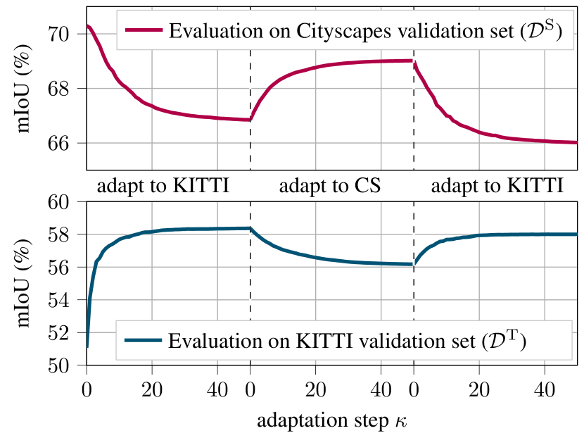
Figure 4: Sequential Adaptation: Performance of UBNA⁺ on the Cityscapes (upper graph) and KITTI (lower graph) validation sets for the adaptation from Cityscapes ($\mathcal{D}^{\mathrm{S}}$) to KITTI ($\mathcal{D}^{\mathrm{T}}$) (left), and after 50 adaptation steps back to Cityscapes ($\mathcal{D}^{\mathrm{T}}$) (middle), then back to KITTI ($\mathcal{D}^{\mathrm{T}}$) (right), in dependence on the number of adaptation batches; VGG-16; mIoU values in %.

While in UDA the primary focus is mostly on a single adaptation to the target domain, it is also of interest to investigate, to what extent this process can be reversed as, e.g., the model should be adapted from day to night and back to day during deployment. As for GTA-5 and SYNTHIA usually the entire dataset is used for training, for this study we use an adaptation setting from Cityscapes to KITTI, where we have available validation sets in both domains and evaluate our VGG-16-based model (cf. Tab. 6) when adapting with UBNA⁺. Fig. 4 shows that while the performance on KITTI ($\mathcal{D}^{\mathrm{T}}$) improves by about $7\%$, the performance on Cityscapes ($\mathcal{D}^{\mathrm{S}}$) decreases by only $3\%$. Interestingly, this effect can even be reversed to a large extent when adapting back to Cityscapes, and even another time, when adapting back to KITTI. This indicates that our approach can be used in a sequential fashion to continuously adapt between two domains as long as the time of domain switch is known (this is needed to re-initialize the momentum factor in (10)).

7 Conclusions

In this work we present the task of “unsupervised domain adaptation (UDA) for semantic segmentation without using source domain representations” and propose our novel Unsupervised BatchNorm Adaptation (UBNA) method as a solution. We show that UBNA works in various settings for UDA, specifically GTA-5 to Cityscapes, SYNTHIA to Cityscapes, and Cityscapes to KITTI, where we improve the VGG-16-based baseline by $5.0\%$, $4.6\%/5.8\%$, and $7.3\%$ absolute, respectively, without the use of any source domain representations for adaptation. We also outperform various baseline approaches, making use of adapting the normalization layers and show that our approach is applicable in an online setting and in a few-shot fashion. Our approach can be beneficial as long as the considered network architecture utilizes batch normalization layers. Under this condition, our UBNA method generalizes over 3 dataset combinations and 6 network architectures by using the same set of hyperparameters, while results can be further improved with UBNA⁺ and dataset-specific hyperparameters. Also, we expect that our method is potentially generalizable to other computer vision tasks and that a combination of our method with domain generalization helps improving further.

Appendix A Additional Experimental Evaluation

With this section our main aim is to provide a more complete overview on the results of our method. This in particular means that we provide a hyperparameter analysis, show our conducted experiments on other source/target domain combinations, provide results for more network architectures, and give a deeper analysis on the variance of different experiments with the same hyperparameter setting but different random seeds. Note that most subsection names are equal to the ones in Sec. 6 of the main paper, and thereby correspond to these respective sections.

A.1 Hyperparameter Analysis

[width=1.0]figs/ablation/momentum_decay_gta_to_cs

Figure 5: Hyperparameter analysis: Performance of UBNA on the Cityscapes validation set for the adaptation from GTA-5 ($\mathcal{D}^{\mathrm{S}}$) to Cityscapes ($\mathcal{D}^{\mathrm{T}}$) in dependence of the batch decay factor $\alpha^{\mathrm{BATCH}}$. Here, $\alpha^{\mathrm{LAYER}}=0.0$ for all UBNA experiments.

[width=1.0]figs/ablation/momentum_decay_synthia_to_cs

Figure 6: Hyperparameter analysis: Performance of UBNA on the Cityscapes validation set for the adaptation from SYNTHIA ($\mathcal{D}^{\mathrm{S}}$) to Cityscapes ($\mathcal{D}^{\mathrm{T}}$) in dependence of the batch decay factor $\alpha^{\mathrm{BATCH}}$. Here, $\alpha^{\mathrm{LAYER}}=0.0$ for all UBNA experiments.

[width=1.0]figs/ablation/momentum_decay_cs_to_kitti

Figure 7: Hyperparameter analysis: Performance of UBNA on the KITTI validation set for the adaptation from Cityscapes ($\mathcal{D}^{\mathrm{S}}$) to KITTI ($\mathcal{D}^{\mathrm{T}}$) in dependence of the batch decay factor $\alpha^{\mathrm{BATCH}}$. Here, $\alpha^{\mathrm{LAYER}}=0.0$ for all UBNA experiments.

[width=1.0]figs/ablation/layer_decay_gta_to_cs

Figure 8: Hyperparameter analysis: Performance of UBNA⁺ on the Cityscapes validation set for the adaptation from GTA-5 ($\mathcal{D}^{\mathrm{S}}$) to Cityscapes ($\mathcal{D}^{\mathrm{T}}$) in dependence of the layer decay factor $\alpha^{\mathrm{LAYER}}$. Here, $\alpha^{\mathrm{BATCH}}=0.08$ for all UBNA⁺ experiments.

[width=1.0]figs/ablation/layer_decay_synthia_to_cs

Figure 9: Hyperparameter analysis: Performance of UBNA⁺ on the Cityscapes validation set for the adaptation from SYNTHIA ($\mathcal{D}^{\mathrm{S}}$) to Cityscapes ($\mathcal{D}^{\mathrm{T}}$) in dependence of the layer decay factor $\alpha^{\mathrm{LAYER}}$. Here, $\alpha^{\mathrm{BATCH}}=0.08$ for all UBNA⁺ experiments.

[width=1.0]figs/ablation/layer_decay_cs_to_kitti

Figure 10: Hyperparameter analysis: Performance of UBNA⁺ on the KITTI validation set for the adaptation from Cityscapes ($\mathcal{D}^{\mathrm{S}}$) to KITTI ($\mathcal{D}^{\mathrm{T}}$) in dependence of the layer decay factor $\alpha^{\mathrm{LAYER}}$. Here, $\alpha^{\mathrm{BATCH}}=0.08$ for all UBNA⁺ experiments.

To give a further insight into the hyperparameter selection for our UBNA method, we show for all three considered dataset settings in Figs. 5, 6, and 7 the performance (ordinate) in dependence of the number of adaptation steps (abscissa). Here, we can already see that the adaptation consistently converges after $\kappa=50$ adaptation steps and a further adaptation does not improve the performance anymore. Note, that Figs. 5, 6, and 7 show the adaptation until $\kappa=100$ adaptation steps, though we do not observe any change in performance after $\kappa=50$ adaptation steps. For $\alpha^{\mathrm{BATCH}}=0.08$, using less adaptation steps could potentially still improve the results (cf. Fig. 5), however, this optimal point does not generalize well across different datasets (cf. Figs. 6 and 12), which is why we use $\kappa=50$ adaptation steps in the main paper, where we observe a stable convergence.

We also show the influence of using different batch-wise decay factors $\alpha^{\mathrm{BATCH}}$. Interestingly, we observe that adapting the statistics to the target domain is beneficial regardless of the used value for $\alpha^{\mathrm{BATCH}}$. However, the convergence is quite optimal for values around $\alpha^{\mathrm{BATCH}}=0.08$. For GTA-5 to Cityscapes (Fig. 5) and SYNTHIA to Cityscapes (Fig. 6), this yields the optimal performance, and for the Cityscapes to KITTI adaptation only a value of $\alpha^{\mathrm{BATCH}}=0.2$ yields a slightly better performance. Much smaller values of $\alpha^{\mathrm{BATCH}}$ lead to an unstable convergence and a lower performance gain (as observed in UBNA⁰ with $\alpha^{\mathrm{BATCH}}=0$, yellow curves in Figs. 5, 6, and 7). On the other hand the more rapidly decreasing BN momentum for larger values of $\alpha^{\mathrm{BATCH}}$ seem to stop the adaptation too rapidly and lead to a convergence much below the optimal point. Still, the approximate optimal hyperparameter values of $\alpha^{\mathrm{BATCH}}=0.08$ and $\kappa=50$ generalize well across different dataset settings, which is essential for practical applications of our UBNA method.

Furthermore, we introduced a layer-wise weighting factor $\alpha^{\mathrm{LAYER}}$, which causes the statistics in the initial layers to be updated more rapidly than in the deeper layers. We show the performance for different values of $\alpha^{\mathrm{LAYER}}$ in Figs. 8, 9, and 10. We observe that for a suitable value of $\alpha^{\mathrm{LAYER}}$ this weighting again improves on top of the UBNA method ($\alpha^{\mathrm{LAYER}}=0$, yellow curves in Figs. 8, 9, and 10), resulting in the UBNA⁺ approach. This could hint at the fact that the domain gap can be compensated to a large extent in the initial layers, which extract domain-specific knowledge, while the deeper layers already learned more domain-invariant features that are rather task-specific. The optimal $\alpha^{\mathrm{LAYER}}$ value of this method is, however, dataset-dependent. On the synthetic-to-real settings GTA-5 to Cityscapes (Fig. 8) and SYNTHIA to Cityscapes (Fig. 9) we found an optimal value of $\alpha^{\mathrm{LAYER}}=0.03$, while for the real-to-real setting Cityscapes to KITTI (Fig. 10) the optimal value was found to be $\alpha^{\mathrm{LAYER}}=0.3$. We suspect that due to the larger domain gap in the synthetic-to-real settings an adaptation only in the initial layers is not sufficient, thereby requiring a smaller value of $\alpha^{\mathrm{LAYER}}$. Conclusively, if one has access to a labelled validation set in the target domain, one can tune this hyperparameter for better performance.

A.2 Comparison to Normalization Approaches

[width=1.0]figs/baseline_comparison/baseline_comparison_gta_to_cs

Figure 11: Comparison to normalization approaches: Performance on the Cityscapes validation set for the adaptation from GTA-5 ($\mathcal{D}^{\mathrm{S}}$) to Cityscapes ($\mathcal{D}^{\mathrm{T}}$) in dependence of the adaptation step $\kappa$ (batch size $B=6$). We also show results when using the statistics from the source domain (no adaptation) and from the target domain (AdaBN by Li et al. [36]).

While our main paper’s comparison regarding baseline approaches was on the adaptation setting from SYNTHIA ($\mathcal{D}^{\mathrm{S}}$) to Cityscapes ($\mathcal{D}^{\mathrm{T}}$), in this part we want to show the same results for the adaptation from GTA-5 ($\mathcal{D}^{\mathrm{S}}$) to Cityscapes ($\mathcal{D}^{\mathrm{T}}$) and from Cityscapes ($\mathcal{D}^{\mathrm{S}}$) to KITTI ($\mathcal{D}^{\mathrm{T}}$) in Figures 11 and 12, respectively. Here, we also observe that the UBNA⁰ method has a peak after adapting with just a few batches, which outperforms the no adaptation and the AdaBN [36] baselines. Using our UBNA method allows convergence of the performance close to or even above this maximum performance, although there might still be a little potential to optimize the hyperparameter $\alpha^{\mathrm{BATCH}}$ for a more stable convergence at the performance maximum. However, for the scope of this paper we rather wanted to show that our hyperparameter setting generalizes to a large degree over different dataset combinations. The more stable convergence of UBNA⁺ also shows that with further hyperparameter tuning, the convergence behavior and maximum performance can even be imporved. In conclusion, this shows that our results observed on other datasets are consistent with the results on the SYNTHIA to Cityscapes adaptation setting.

[width=1.0]figs/baseline_comparison/baseline_comparison_cs_to_kitti

Figure 12: Comparison to normalization approaches: Performance on the KITTI validation set for the adaptation from Cityscapes ($\mathcal{D}^{\mathrm{S}}$) to KITTI ($\mathcal{D}^{\mathrm{T}}$) in dependence of the adaptation step $\kappa$ (batch size $B=6$). We also show results when using the statistics from the source domain (no adaptation) and from the target domain (AdaBN by Li et al. [36]).

A.3 Comparison to UDA Approaches

Table 8: Comparison to UDA approaches: Performance of UBNA and UBNA⁺ in comparison to UDA methods on the Cityscapes validation set for the adaptation from GTA-5 ($\mathcal{D}^{\mathrm{S}}$) to Cityscapes ($\mathcal{D}^{\mathrm{T}}$). We evaluate different models (first column), compare different methods (second column, values from the respective papers), show if they use labeled source data during unsupervised domain adaptation (third column), evaluate the IoU performance (%) on the single semantic classes, and finally give an mIoU (%) over 19 classes. For ResNet results we use the ResNet-50 topology, as this yielded better results at lower computational complexity compared to the ResNet-101 often used in UDA approaches. Best results for UDA and for UDA without source data are printed in boldface.

Network	Method	Source data during [-0.07cm] adaptation	road	sidewalk	building	wall∗∗	fence∗∗	pole∗∗	traffic light	traffic sign	vegetation	terrain∗	sky	person	rider	car	truck∗	bus	on rails∗	motorbike	bike	$\mathrm{mIoU}$ (%) (19 classes)
ResNet-50	Du et al. [11]	yes	90.3	38.9	81.7	24.8	22.9	30.5	37.0	21.2	84.8	38.8	76.9	58.8	30.7	85.7	30.6	38.1	5.9	28.3	36.9	45.4
	Vu et al. [67]	yes	89.4	33.1	81.0	26.6	26.8	27.2	33.5	24.7	83.9	36.7	78.8	58.7	30.5	84.8	38.5	44.5	1.7	31.6	32.4	45.5
	Li et al. [38]	yes	91.0	44.7	84.2	34.6	27.6	30.2	36.0	36.0	85.0	43.6	83.0	58.6	31.6	83.3	35.3	49.7	3.3	28.8	35.6	48.5
	Dong et al. [9]	yes	89.6	50.4	83.0	35.6	26.9	31.1	37.3	35.1	83.5	40.6	84.0	60.6	34.3	80.9	35.1	47.3	0.5	34.5	33.7	48.6
	Wang et al. [70]	yes	90.6	44.7	84.8	34.3	28.7	31.6	35.0	37.6	84.7	43.3	85.3	57.0	31.5	83.8	42.6	48.5	1.9	30.4	39.0	49.2
	Yang et al. [74]	yes	90.8	41.4	84.7	35.1	27.5	31.2	38.0	32.8	85.6	42.1	84.9	59.6	34.4	85.0	42.8	52.7	3.4	30.9	38.1	49.5
	Zhang et al. [79]	yes	90.4	51.6	83.8	34.2	27.8	38.4	25.3	48.4	85.4	38.2	78.1	58.6	34.6	84.7	21.9	42.7	41.1	29.3	37.2	50.2
	Kim et al. [25]	yes	92.9	55.0	85.3	34.2	31.1	34.9	40.7	34.0	85.2	40.1	87.1	61.0	31.1	82.5	32.3	42.9	0.3	36.4	46.1	50.2
	Yang et al. [75]	yes	92.5	53.3	82.4	26.5	27.6	36.4	40.6	38.9	82.3	39.8	78.0	62.6	34.4	84.9	34.1	53.1	16.9	27.7	46.4	50.5
	Mei et al. [44]	yes	94.1	58.8	85.4	39.7	29.2	25.1	43.1	34.2	84.8	34.6	88.7	62.7	30.3	87.6	42.3	50.3	24.7	35.2	40.2	52.2
	No adaptation	-	58.1	23.8	70.5	14.8	19.2	30.5	29.0	17.7	79.1	21.8	83.1	56.4	14.8	72.3	19.5	4.5	0.9	16.5	5.6	33.6
	UBNA	no	81.8	32.3	79.5	18.2	23.8	34.9	29.5	19.8	74.2	17.9	82.4	57.5	11.1	81.6	16.1	19.0	2.5	21.3	9.8	37.5
	UBNA+	no	70.6	25.8	78.5	17.7	23.7	34.2	28.9	19.0	77.8	19.6	82.6	57.4	11.5	81.5	16.9	17.1	1.0	20.6	9.1	36.5
VGG-16	Vu et al. [67]	yes	86.9	28.7	78.7	28.5	25.2	17.1	20.3	10.9	80.0	26.4	70.2	47.1	8.4	81.5	26.0	17.2	18.9	11.7	1.6	36.1
	Du et al. [11]	yes	88.7	32.1	79.5	29.9	22.0	23.8	21.7	10.7	80.8	29.8	72.5	49.5	16.1	82.1	23.2	18.1	3.5	24.4	8.1	37.7
	Li et al. [38]	yes	89.2	40.9	81.2	29.1	19.2	14.2	29.0	19.6	83.7	35.9	80.7	54.7	23.3	82.7	25.8	28.0	2.3	25.7	19.9	41.3
	Dong et al. [9]	yes	89.8	46.1	75.2	30.1	27.9	15.0	20.4	18.9	82.6	39.1	77.6	47.8	17.4	76.2	28.5	33.4	0.5	29.4	30.8	41.4
	Yang et al. [75]	yes	86.1	35.1	80.6	30.8	20.4	27.5	30.0	26.0	82.1	30.3	73.6	52.5	21.7	81.7	24.0	30.5	29.9	14.6	24.0	42.2
	Kim et al. [25]	yes	92.5	54.5	83.9	34.5	25.5	31.0	30.4	18.0	84.1	39.6	83.9	53.6	19.3	81.7	21.1	13.6	17.7	12.3	6.5	42.3
	Wang et al. [70]	yes	88.1	35.8	83.1	25.8	23.9	29.2	28.8	28.6	83.0	36.7	82.3	53.7	22.8	82.3	26.4	38.6	0.0	19.6	17.1	42.4
	Choi et al. [6]	yes	90.2	51.5	81.1	15.0	10.7	37.5	35.2	28.9	84.1	32.7	75.9	62.7	19.9	82.6	22.9	28.3	0.0	23.0	25.4	42.5
	Yang et al. [74]	yes	90.1	41.2	82.2	30.3	21.3	18.3	33.5	23.0	84.1	37.5	81.4	54.2	24.3	83.0	27.6	32.0	8.1	29.7	26.9	43.6
	No adaptation	-	55.8	21.9	65.9	15.2	14.7	27.5	31.0	17.9	77.8	19.5	74.4	55.2	12.1	71.7	11.9	3.3	0.5	13.2	9.6	31.5
	UBNA	no	80.8	29.4	77.6	19.8	17.1	33.9	29.3	20.5	73.9	16.8	76.7	58.3	15.2	79.1	13.6	12.5	5.7	14.1	10.8	36.1
	UBNA+	no	79.9	29.9	78.1	21.1	16.5	33.8	29.7	20.6	75.6	18.4	78.0	58.4	14.6	79.4	14.8	13.0	5.8	14.6	10.6	36.5

Table 9: Comparison to UDA approaches: Performance of UBNA and UBNA⁺ in comparison to UDA methods on the Cityscapes validation set for the adaptation from SYNTHIA ($\mathcal{D}^{\mathrm{S}}$) to Cityscapes ($\mathcal{D}^{\mathrm{T}}$). We evaluate different models (first column), compare different methods (second columns, values from the respective papers), show if they use labeled source data during unsupervised domain adaptation (third column), evaluate the IoU performance (%) on the single semantic classes, and finally give an mIoU (%) over 13 classes and over 16 classes (the latter including also wall, fence and pole) as in [31, 67]. For ResNet results we use the ResNet-50 topology, as this yielded better results at lower computational complexity compared to the ResNet-101 commonly used in other approaches. Best UDA results and best UDA without source data results are printed in boldface.

Network	Method	Source data during [-0.07cm] adaptation	road	sidewalk	building	wall∗∗	fence∗∗	pole∗∗	traffic light	traffic sign	vegetation	terrain∗	sky	person	rider	car	truck∗	bus	on rails∗	motorbike	bike	$\mathrm{mIoU}$ (%) (16 classes)	$\mathrm{mIoU}$ (%) (13 classes)
ResNet-50	Vu et al. [67]	yes	85.6	42.2	79.7	8.7	0.4	25.9	5.4	8.1	80.4	-	84.1	57.9	23.8	73.3	-	36.4	-	14.2	33.0	41.2	48.0
	Du et al. [11]	yes	84.6	41.7	80.8	-	-	-	11.5	14.7	80.8	-	85.3	57.5	21.6	82.0	-	36.0	-	19.3	34.5	-	50.0
	Li et al. [38]	yes	86.0	46.7	80.3	-	-	-	14.1	11.6	79.2	-	81.3	54.1	27.9	73.7	-	42.2	-	25.7	45.3	-	51.4
	Wang et al. [70]	yes	83.0	44.0	80.3	-	-	-	17.1	15.8	80.5	-	81.8	59.9	33.1	70.2	-	37.3	-	28.5	45.8	-	52.1
	Yang et al. [74]	yes	85.1	44.5	81.0	-	-	-	16.4	15.2	80.1	-	84.8	59.4	31.9	73.2	-	41.0	-	32.6	44.7	-	53.1
	Dong et al. [9]	yes	80.2	41.1	78.9	23.6	0.6	31.0	27.1	29.5	82.5	-	83.2	62.1	26.8	81.5	-	37.2	-	27.3	42.9	47.2	-
	Mei et al. [44]	yes	81.9	41.5	83.3	17.7	4.6	32.3	30.9	28.8	83.4	-	85.0	65.5	30.8	86.5	-	38.2	-	33.1	52.7	49.8	57.0
	No adaptation	-	36.5	18.6	68.3	2.0	0.2	30.3	6.0	10.2	74.5	-	81.6	51.9	10.6	41.3	-	9.5	-	2.2	22.6	29.1	34.1
	UBNA	no	62.5	22.8	75.6	3.1	0.5	32.5	8.6	11.3	73.0	-	82.7	42.5	12.5	67.1	-	12.5	-	5.7	27.8	33.8	39.7
	UBNA+	no	57.4	22.3	75.0	3.6	0.4	33.8	8.5	11.1	76.2	-	82.6	46.8	12.8	61.2	-	12.8	-	4.8	28.5	33.6	39.4
VGG-16	Vu et al. [67]	yes	67.9	29.4	71.9	6.3	0.3	19.9	0.6	2.6	-	74.9	74.9	35.4	9.6	67.8	-	21.4	-	4.1	15.5	31.4	36.6
	Lee et al. [31]	yes	71.1	29.8	71.4	3.7	0.3	33.2	6.4	15.6	81.2	-	78.9	52.7	13.1	75.9	-	25.5	-	10.0	20.5	36.8	42.4
	Dong et al. [9]	yes	70.9	30.5	77.8	9.0	0.6	27.3	8.8	12.9	74.8	-	81.1	43.0	25.1	73.4	-	34.5	-	19.5	38.2	39.2	-
	Yang et al. [74]	yes	73.7	29.6	77.6	1.0	0.4	26.0	14.7	26.6	80.6	-	81.8	57.2	24.5	76.1	-	27.6	-	13.6	46.6	41.1	-
	No adaptation	-	49.4	20.8	61.5	3.6	0.1	30.5	13.6	14.1	74.4	-	75.5	53.5	10.6	47.2	-	4.8	-	3.0	17.1	30.0	35.2
	UBNA	no	72.3	26.6	73.0	2.3	0.3	31.5	12.1	16.6	72.1	-	75.6	45.4	13.6	61.2	-	8.5	-	8.5	30.1	34.4	40.7
	UBNA+	no	71.5	27.3	72.9	2.5	0.3	32.0	12.7	16.7	74.6	-	75.4	47.1	13.6	61.4	-	8.5	-	8.3	29.2	34.6	41.0

To facilitate a more extensive comparison with respect to past and future works, we extend our comparison to UDA baseline approaches also to models using a ResNet-based network architecture, which we demonstrate in Tables 8 and 9. For our experiments we use a ResNet-50 backbone, which provides a good trade-off between computational complexity and performance. When analyzing the results we observe that UBNA improves the final model performance by 3.9% and 4.7/5.6% absolute for the adaptations from GTA-5 to Cityscapes and SYNTHIA to Cityscapes, respectively. Additionally, the performance on the single classes improves for the large majority of classes. This is in consistency with the results obtained using a VGG-16-based model. Interestingly, for ResNet-50, the UBNA⁺ method does not give an improvement over UBNA, as the hyperparameters were optimized for the VGG-16 backbone. Accordingly, we can see that UBNA has a higher degree of generalization over different network architectures, while UBNA⁺ is a bit more hyperparameter-sensitive.

A.4 Few-Shot Capability

To give further insight into the number of images necessary to obtain a stable adaptation using just a few images as shown in Tab. 4, in Figures 13 and 14 we show the mean value as well as the standard deviation over the results from ten experiments. We observe that the standard deviation is quite high for only one or two images per batch. The performance slightly increases for three or more images per adaptation batch. To reduce the dependency on a single image, at least three images should be chosen for adaptation, as from this number on, the standard deviation of different experiments is significantly lower and the final performance significantly higher as can be seen in Figures 13 and 14.

A.5 Ablation Studies

[width=1.0]figs/few_shot/few_shot_gta_variance_ubna_plus

Figure 13: Few-shot adaptation: Performance of UBNA⁺ on the Cityscapes validation set for the adaptation from GTA-5 ($\mathcal{D}^{\mathrm{S}}$) to Cityscapes ($\mathcal{D}^{\mathrm{T}}$) for different numbers of total images used for adaptation. We show the mean and the standard deviation over 10 different experiments after the $\kappa=50$th step, whereby in each experiment all batches contain the same image(s).

[width=1.0]figs/few_shot/few_shot_synthia_variance_ubna_plus

Figure 14: Few-shot adaptation: Performance of UBNA⁺ on the Cityscapes validation set for the adaptation from SYNTHIA ($\mathcal{D}^{\mathrm{S}}$) to Cityscapes ($\mathcal{D}^{\mathrm{T}}$) for different numbers of total images used for adaptation. We show the mean and the standard deviation over 10 different experiments after the $\kappa=50$th step, whereby in each experiment all batches contain the same image(s).

Table 10: Network topology ablation: Performance of UBNA⁰, UBNA, and UBNA⁺ on the Cityscapes validation set for the adaptation from GTA-5 ($\mathcal{D}^{\mathrm{S}}$) to Cityscapes ($\mathcal{D}^{\mathrm{T}}$) for various network topologies; best results for each network topology in boldface; mIoU values in %; batch size $B=6$; $\alpha^{\mathrm{BATCH}}=0.08$ (UBNA, UBNA⁺); $\alpha^{\mathrm{LAYER}}=0.03$ (UBNA⁺).

Network	No adaptation	UBNA0	UBNA	UBNA+
VGG-16	31.5	33.9	36.1	36.5
VGG-19	31.2	35.3	37.4	37.5
ResNet-18	34.1	29.4	34.8	35.5
ResNet-34	33.6	34.3	36.0	35.5
ResNet-50	33.6	35.6	37.5	36.5
ResNet-101	30.0	33.4	34.6	32.6

Table 11: Network topology ablation: Performance of UBNA⁰, UBNA, and UBNA⁺ on the Cityscapes validation set for the adaptation from SYNTHIA ($\mathcal{D}^{\mathbf{S}}$) to Cityscapes ($\mathcal{D}^{\mathrm{T}}$) for various network topologies; best results for each network topology in boldface; mIoU values in %; batch size $B=6$; $\alpha^{\mathrm{BATCH}}=0.08$ (UBNA, UBNA⁺); $\alpha^{\mathrm{LAYER}}=0.03$ (UBNA⁺).

Network	No adaptation	UBNA0	UBNA	UBNA+
VGG-16	30.0	32.6	34.4	34.6
VGG-19	30.9	29.1	30.8	31.7
ResNet-18	28.6	31.3	31.9	31.7
ResNet-34	27.4	30.1	30.0	30.3
ResNet-50	29.1	32.9	33.8	33.6
ResNet-101	30.8	30.0	31.8	34.3

While the layer-wise weighting (UBNA⁺) worked particularly well in the real-to-real adaptation setting (cf. Tab. 7), the success on settings with a larger domain gap is a little ambiguous, as can be seen in Tables 10 and 11. While the UBNA⁺ method always improves on top of the non-adapted baseline, we observe that the performance gains over the UBNA method are rather small and in some cases, we even observe a better performance with UBNA (e.g., the last three rows in Tab. 10). Also, we had to reduce the layer-wise weighting factor by a factor of $10$ to a value $\alpha^{\mathrm{LAYER}}=\mathrm{0.03}$ to obtain decent results, which shows the higher hyperparameter dependency compared to the plain UBNA method. Therefore, on a new setting we would recommend to start with the UBNA method and (if possible) tune afterwards with the layer-wise weighting characterizing our UBNA⁺ method.

Appendix B Additional Qualitative Results

To emphasize also the qualitative effects our method has on the results, we show images of the adaptations from GTA-5 ($\mathcal{D}^{\mathrm{S}}$) to Cityscapes ($\mathcal{D}^{\mathrm{T}}$), SYNTHIA ($\mathcal{D}^{\mathrm{S}}$) to Cityscapes ($\mathcal{D}^{\mathrm{T}}$), and Cityscapes ($\mathcal{D}^{\mathrm{S}}$) to KITTI ($\mathcal{D}^{\mathrm{T}}$) in Figures 15, 16, and 17, respectively. In these figures, we show the input images, the ground truth segmentation mask, the predicted segmentation mask when using the model without adaptation, and the results from the adapted model using the UBNA method, from left to right. Interestingly, the qualitative effects are quite similar for all three dataset setups as already observed in the class-wise improvements in Sec. 9. First of all, the overall artifacts present in different parts of the image are significantly reduced, which is especially well observable on the synthetic-to-real adaptation (e.g., Fig. 15, row 1, or Fig. 16, row 4). However, even in the real-to-real adaptation setting, where the baseline approach already is significantly better, we observe that artifacts are removed by UBNA⁺ from the image, as visible in the last three rows of Fig. 17, where the human-class artifact in the center of the image is removed. Also, in all three dataset setups, the detection of the road class is significantly improved (e.g. Fig. 15, rows 4 and 5). Also, cars are better distinguished from their surrounding and less wrongfully predicted cars are present in the semantic segmentation prediction (e.g. Fig. 16, rows 6 and 7). Nevertheless, there are also some classes that are not detected as good as before (cf. Tables 8 and 9) which is also visible qualitatively, e.g., the vegetation class contains slightly more artifacts than before the adaptation (cf. Fig. 16, row 2).

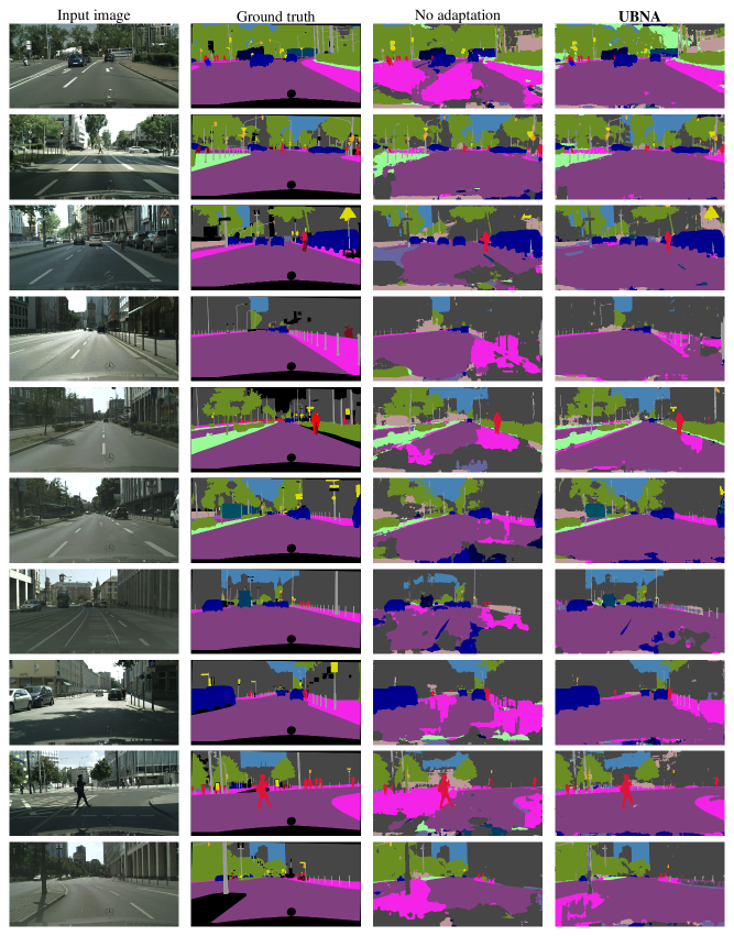
Figure 15: Qualitative comparison: Qualitative results of UBNA in comparison to no adaptation and the ground truth on the Cityscapes validation set for the adaptation from GTA-5 ($\mathcal{D}^{\mathrm{S}}$) to Cityscapes ($\mathcal{D}^{\mathrm{T}}$). The figure is best viewed on screen and in color.

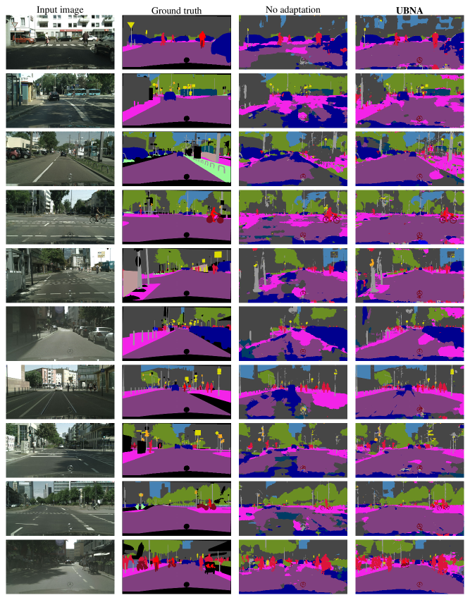
Figure 16: Qualitative comparison: Qualitative results of UBNA in comparison to no adaptation and the ground truth on the Cityscapes validation set for the adaptation from SYNTHIA ($\mathcal{D}^{\mathrm{S}}$) to Cityscapes ($\mathcal{D}^{\mathrm{T}}$). The figure is best viewed on screen and in color.

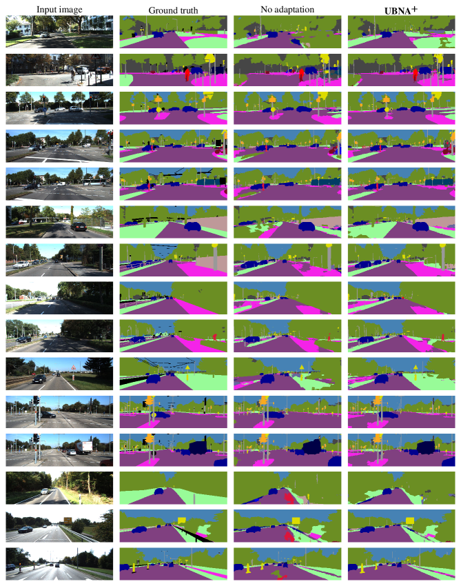
Figure 17: Qualitative comparison: Qualitative results of UBNA⁺ ($\alpha^{\mathrm{LAYER}}=0.3$) in comparison to no adaptation and the ground truth on the KITTI validation set for the adaptation from Cityscapes ($\mathcal{D}^{\mathrm{S}}$) to KITTI ($\mathcal{D}^{\mathrm{T}}$). The figure is best viewed on screen and in color.

References

- [1] Jimmy Lei Ba, Jamie Ryan Kiros, and Geoffrey E. Hinton. Layer Normalization. arXiv, July 2016.
- [2] Mathilde Bateson, Hoel Kervadec, Jose Dolz, Hervé Lombaert, and Ismail Ben Ayed. Source-Relaxed Domain Adaptation for Image Segmentation. In Proc. of MICCAI, pages 490–499, Lima, Peru, Oct. 2020.
- [3] Jan-Aike Bolte, Markus Kamp, Antonia Breuer, Silviu Homoceanu, Peter Schlicht, Fabian Hüger, Daniel Lipinski, and Tim Fingscheidt. Unsupervised Domain Adaptation to Improve Image Segmentation Quality Both in the Source and Target Domain. In Proc. of CVPR - Workshops, pages 1404–1413, Long Beach, CA, USA, June 2019.
- [4] Woong-Gi Chang, Tackgeun You, Seonguk Seo, Suha Kwak, and Bohyung Han. Domain-Specific Batch Normalization for Unsupervised Domain Adaptation. In Proc. of CVPR, pages 7354–7362, Long Beach, CA, USA, June 2019.
- [5] Minghao Chen, Hongyang Xue, and Deng Cai. Domain Adaptation for Semantic Segmentation With Maximum Squares Loss. In Proc. of ICCV, pages 2090–2099, Seoul, Korea, Oct. 2019.
- [6] Jaehoon Choi, Taekyung Kim, and Changick Kim. Self-Ensembling With GAN-Based Data Augmentation for Domain Adaptation in Semantic Segmentation. In Proc. of ICCV, pages 6830–6840, Seoul, Korea, Oct. 2019.
- [7] Sungha Choi, Sanghun Jung, Huiwon Yun, Joanne T. Kim, Seungryong Kim, and Jaegul Choo. RobustNet: Improving Domain Generalization in Urban-Scene Segmentation via Instance Selective Whitening. In Proc. of CVPR, pages 11580–11590, Virtual, June 2021.
- [8] Marius Cordts, Mohamed Omran, Sebastian Ramos, Timo Rehfeld, Markus Enzweiler, Rodrigo Benenson, Uwe Franke, Stefan Roth, and Bernt Schiele. The Cityscapes Dataset for Semantic Urban Scene Understanding. In Proc. of CVPR, pages 3213–3223, Las Vegas, NV, USA, June 2016.
- [9] Jiahua Dong, Yang Cong, Gan Sun, Yuyang Liu, and Xiaowei Xu. CSCL: Critical Semantic-Consistent Learning for Unsupervised Domain Adaptation. In Proc. of ECCV, pages 745–762, Glasgow, UK, Aug. 2020.
- [10] Qi Dou, Daniel Coelho de Castro, Konstantinos Kamnitsas, and Ben Glocker. Domain Generalization via Model-Agnostic Learning of Semantic Features. In Proc. of NeurIPS, pages 6447–6458, Vancouver, Canada, Dec. 2019.
- [11] Liang Du, Jingang Tan, Hongye Yang, Jianfeng Feng, Xiangyang Xue, Qibao Zheng, Xiaoqing Ye, and Xiaolin Zhang. SSF-DAN: Separated Semantic Feature Based Domain Adaptation Network for Semantic Segmentation. In Proc. of ICCV, pages 982–991, Seoul, Korea, Oct. 2019.
- [12] Mark Everingham, Luc Van Gool, Christopher K. I. Williams, John Winn, and Andrew Zisserman. The Pascal Visual Object Classes Challenge: A Retrospective. International Journal of Computer Vision (IJCV), 111(1):98–136, Jan. 2015.
- [13] Yaroslav Ganin and Victor Lempitsky. Unsupervised Domain Adaptation by Backpropagation. In Proc. of ICML, pages 1180–1189, Lille, France, July 2015.
- [14] Andreas Geiger, Philip Lenz, Christoph Stiller, and Raquel Urtasun. Vision Meets Robotics: The KITTI Dataset. International Journal of Robotics Research (IJRR), 32(11):1231–1237, Aug. 2013.
- [15] Clément Godard, Oisin Mac Aodha, Michael Firman, and Gabriel J. Brostow. Digging Into Self-Supervised Monocular Depth Estimation. In Proc. of ICCV, pages 3828–3838, Seoul, Korea, Oct. 2019.
- [16] Rui Gong, Wen Li, Yuhua Chen, and Luc Van Gool. DLOW: Domain Flow for Adaptation and Generalization. In Proc. of CVPR, pages 2477–2486, Long Beach, CA, USA, June 2019.
- [17] Kaiming He, Xiangyu Zhang, Shaoqing Ren, and Jian Sun. Deep Residual Learning for Image Recognition. In Proc. of CVPR, pages 770–778, Las Vegas, NV, USA, June 2016.
- [18] Judy Hoffman, Eric Tzeng, Taesung Park, Jun-Yan Zhu, Philip Isola, Kate Saenko, Alexei A. Efros, and Trevor Darrell. CyCADA: Cycle-Consistent Adversarial Domain Adaptation. In Proc. of ICML, pages 1989–1998, Stockholm, Sweden, July 2018.
- [19] Judy Hoffman, Dequan Wang, Fischer Yu, and Trevor Darrell. FCNs in the Wild: Pixel-Level Adversarial and Constraint-Based Adaptation. arXiv, (1612.02649), Dec. 2016.
- [20] Jiaxing Huang, Shijian Lu, Dayan Guan, and Xiaobing Zhang. Contextual-Relation Consistent Domain Adaptation for Semantic Segmentation. In Proc of ECCV, pages 705–722, Glasow, UK, Aug. 2020.
- [21] Xun Huang and Serge Belongie. Arbitrary Style Transfer in Real-Time With Adaptive Instance Normalization. In Proc. of ICCV, pages 1501–1510, Venice, Italy, Oct. 2017.
- [22] Sergey Ioffe. Batch Renormalization: Towards Reducing Minibatch Dependence in Batch-Normalized Models. In Proc. of NIPS, pages 1945–1953, Long Beach, CA, USA, Dec. 2017.
- [23] Sergey Ioffe and Christian Szegedy. Batch Normalization: Accelerating Deep Network Training by Reducing Internal Covariate Shift. In Proc. of ICML, pages 448–456, Lille, France, July 2015.
- [24] H. Jung, J. Ju, M. Jung, and J. Kim. Less-Forgetting Learning in Deep Neural Networks. arXiv, (1607.00122), 2016.
- [25] Myeongjin Kim and Hyeran Byun. Learning Texture Invariant Representation for Domain Adaptation of Semantic Segmentation. In Proc. of CVPR, pages 12975–12984, Seattle, WA, USA, June 2020.
- [26] Diederik P. Kingma and Jimmy Ba. Adam: A Method for Stochastic Optimization. In Proc. of ICLR, pages 1–15, San Diego, CA, USA, May 2015.
- [27] J. Kirkpatrick, R. Pascanu, N. Rabinowitz, J. Veness, G. Desjardins, A. A. Rusu, K. Milan, J. Quan, T. Ramalho, A. Grabska-Barwinska, D. Hassabis, C. Clopath, D. Kumarana, and R. Hadsella. Overcoming Catastrophic Forgetting in Neural Networks. Proceedings of the National Academy of Sciences, 114(13):3521–3526, 2016.
- [28] Marvin Klingner, Andreas Bär, and Tim Fingscheidt. Improved Noise and Attack Robustness for Semantic Segmentation by Using Multi-Task Training with Self-Supervised Depth Estimation. In Proc. of CVPR - Workshops, pages 1299–1309, Seattle, WA, USA, June 2020.
- [29] Marvin Klingner, Jan-Aike Termöhlen, Jonas Mikolajczyk, and Tim Fingscheidt. Self-Supervised Monocular Depth Estimation: Solving the Dynamic Object Problem by Semantic Guidance. In Proc. of ECCV, pages 582–600, Glasgow, UK, Aug. 2020.
- [30] Vinod K. Kurmi, Venkatesh K. Subramanian, and Vinay P. Namboodiri. Domain Impression: A Source Data Free Domain Adaptation Method. In Proc. of WACV, pages 615–625, Virtual Conference, Jan. 2021.
- [31] Kuan-Hui Lee, German Ros, Jie Li, and Adrien Gaidon. SPIGAN: Privileged Adversarial Learning from Simulation. In Proc. of ICLR, pages 1–14, New Orleans, LA, USA, Apr. 2019.
- [32] Da Li, Jianshu Zhang, Yongxin Yang, Cong Liu, Yi-Zhe Song, and Timothy M. Hospedales. Episodic Training for Domain Generalization. In Proc. of ICCV, pages 1446–1455, Seoul, Korea, Oct. 2019.
- [33] Rui Li, Qianfen Jiao, Wenming Cao, Hau-San Wong, and Si Wu. Model Adaptation: Unsupervised Domain Adaptation Without Source Data. In Proc. of CVPR, pages 9641–9650, Seattle, WA, USA, June 2020.
- [34] Shunkai Li, Xin Wang, Yingdian Cao, Fei Xue, Zike Yan, and Hongbin Zha. Self-Supervised Deep Visual Odometry With Online Adaptation. In Proc. of CVPR, pages 6339–6348, Seattle, WA, USA, June 2020.
- [35] Xianfeng Li, Weijie Chen, Di Xie, Shicai Yang, Peng Yuan, Shiliang Pu, and Yueting Zhuang. A Free Lunch for Unsupervised Domain Adaptive Object Detection Without Source Data. In Proc. of AAAI, pages xxxx–xxxx, Virtual Conference, Feb. 2021.
- [36] Yanghao Li, Naiyan Wang, Jianping Shi, Xiaodi Hou, and Jiaying Liu. Adaptive Batch Normalization for Practical Domain Adaptation. Pattern Recognition, 80:109–117, Aug. 2018.
- [37] Yanghao Li, Naiyan Wang, Jianping Shi, Jiaying Liu, and Xiaodi Hou. Revisiting Batch Normalization for Practical Domain Adaptation. In Proc. of ICLR - Workshops, pages 1–10, Toulon, France, Apr. 2017.
- [38] Yunsheng Li, Lu Yuan, and Nuno Vasconcelos. Bidirectional Learning for Domain Adaptation of Semantic Segmentation. In Proc. of CVPR, pages 6936–6945, Long Beach, CA, USA, June 2019.
- [39] Jian Liang, Dapeng Hu, and Jiashi Feng. Do We Really Need to Access the Source Data? Source Hypothesis Transfer for Unsupervised Domain Adaptation. In Proc. of ICML, pages 6028–6039, Virtual Conference, July 2020.
- [40] Tsung-Yi Lin, Michael Maire, Serge Belongie, James Hays, Pietro Perona, Deva Ramanan, Piotr Dollár, and C Lawrence Zitnick. Microsoft COCO: Common Objects in Context. In Proc. of ECCV, pages 740–755, Zurich, Switzerland, Sept. 2014.
- [41] Yuang Liu, Wei Zhang, and Jun Wang. Source-Free Domain Adaptation for Semantic Segmentation. In Proc. of CVPR, pages 1215–1224, Virtual, June 2021.
- [42] Massimiliano Mancini, Lorenzo Porzi, Samuel Rota Bulò, Barbara Caputo, and Elisa Ricci. Boosting Domain Adaptation by Discovering Latent Domains. In Proc. of CVPR, pages 3771–3780, Salt Lake City, UT, USA, June 2018.
- [43] Fabio Maria Carlucci, Lorenzo Porzi, Barbara Caputo, Elisa Ricci, and Samuel Rota Bulo. AutoDIAL: Automatic DomaIn Alignment Layers. In Proc. of ICCV, pages 5067–5075, Venice, Italy, Oct. 2017.
- [44] Ke Mei, Chuang Zhu, Jiaqi Zou, and Shanghang Zhang. Instance Adaptive Self-Training for Unsupervised Domain Adaptation. In Proc. of ECCV, pages 415–430, Glasgow, UK, Aug. 2020.
- [45] Moritz Menze and Andreas Geiger. Object Scene Flow for Autonomous Vehicles. In Proc. of CVPR, pages 3061–3070, Boston, MA, USA, June 2015.
- [46] Takeru Miyato, Toshiki Kataoka, Masanori Koyama, and Yuichi Yoshida. Spectral Normalization for Generative Adversarial Networks. In Proc. of ICLR, pages 1–12, Vancouver, BC, Canada, Apr. 2018.
- [47] Hyeonseob Nam and Hyo-Eun Kim. Batch-Instance Normalization for Adaptively Style-Invariant Neural Network. In Proc. of NIPS, pages 2558–2567, Montréal, QC, Canada, Dec. 2018.
- [48] Gerhard Neuhold, Tobias Ollmann, Samuel Rota Bulò, and Peter Kontschieder. The Mapillary Vistas Dataset for Semantic Understanding of Street Scenes. In Proc. of ICCV, pages 4990–4999, Venice, Italy, Oct. 2017.
- [49] Xingang Pan, Ping Luo, Jianping Shi, and Xiaoou Tang. Two at Once: Enhancing Learning and Generalization Capacities via IBN-Net. In Proc. of ECCV, pages 464–479, Munich, Germany, Sept. 2018.
- [50] Adam Paszke, Sam Gross, Francisco Massa, Adam Lerer, James Bradbury, Gregory Chanan, Trevor Killeen, Zeming Lin, Natalia Gimelshein, Luca Antiga, Alban Desmaison, et al. PyTorch: An Imperative Style, High-Performance Deep Learning Library. In Proc. of NeurIPS, pages 8024–8035, Vancouver, BC, Canada, Dec. 2019.
- [51] Varun Ravi Kumar, Marvin Klingner, Senthil Yogamani, Markus Bach, Stefan Milz, Tim Fingscheidt, and Patrick Mäder. SVDistNet: Self-Supervised Near-Field Distance Estimation on Surround View Fisheye Cameras. IEEE Transactions on Intelligent Transportation Systems, pages 1–10, 2021.
- [52] Varun Ravi Kumar, Marvin Klingner, Senthil Yogamani, Stefan Milz, Tim Fingscheidt, and Patrick Mäder. SynDistNet: Self-Supervised Monocular Fisheye Camera Distance Estimation Synergized with Semantic Segmentation for Autonomous Driving. In Proc. of WACV, pages 61–71, Waikoloa, HI, USA, Jan. 2021.
- [53] Stephan Richter, Vibhav Vineet, Stefan Roth, and Vladlen Koltun. Playing for Data: Ground Truth from Computer Games. In Proc. of ECCV, pages 102–118, Amsterdam, Netherlands, Oct. 2016.
- [54] Rob Romijnders, Panagiotis Meletis, and Gijs Dubbelman. A Domain Agnostic Normalization Layer for Unsupervised Adversarial Domain Adaptation. In Proc. of WACV, pages 1866–1875, Waikoloa, Hawaii, Jan. 2019.
- [55] German Ros, Laura Sellart, Joanna Materzynska, David Vazquez, and Antonio M. Lopez. The SYNTHIA Dataset: A Large Collection of Synthetic Images for Semantic Segmentation of Urban Scenes. In Proc. of CVPR, pages 3234–3243, Las Vegas, NV, USA, June 2016.
- [56] Olga Russakovsky, Jia Deng, Hao Su, Jonathan Krause, Sanjeev Satheesh, Sean Ma, Zhiheng Huang, Andrej Karpathy, Aditya Khosla, Michael Bernstein, Alexander C. Berg, and Li Fei-Fei. ImageNet Large Scale Visual Recognition Challenge. International Journal of Computer Vision (IJCV), 115(3):211–252, Dec. 2015.
- [57] Steffen Schneider, Evgenia Rusak, Luisa Eck, Oliver Bringmann, Wieland Brendel, and Matthias Bethge. Improving Robustness Against Common Corruptions by Covariate Shift Adaptation. In Proc. of NeurIPS, pages 1–13, Virtual Conference, Dec. 2020.
- [58] Seonguk Seo, Yumin Suh, Dongwan Kim, Geeho Kim, Jongwoo Han, and Bohyung Han. Learning to Optimize Domain Specific Normalization for Domain Generalization. In Proc. of ECCV, pages 68–83, Glasgow, UK, Aug. 2020.
- [59] Wenqi Shao, Tianjian Meng, Jingyu Li, Ruimao Zhang, Yudian Li, Xiaogang Wang, and Ping Luo. SSN: Learning Sparse Switchable Normalization via SparsestMax. In Proc. of CVPR, pages 443–451, Long Beach, CA, USA, June 2019.
- [60] Karen Simonyan and Andrew Zisserman. Very Deep Convolutional Networks for Large-Scale Image Recognition. In Proc. of ICLR, pages 1–27, San Diego, CA, USA, May 2015.
- [61] Muhammad Naseer Subhani and Mohsen Ali. Learning from Scale-Invariant Examples for Domain Adaptation in Semantic Segmentation. In Proc. of ECCV, pages 290–306, Glasgow, UK, Aug. 2020.
- [62] Prabhu Teja S and Francois Fleuret. Uncertainty Reduction for Model Adaptation in Semantic Segmentation. In Proc. of CVPR, pages 9613–9623, Virtual, June 2021.
- [63] Jan-Aike Termöhlen, Marvin Klingner, Leon J. Brettin, Nico M. Schmidt, and Tim Fingscheidt. Continual Unsupervised Domain Adaptation for Semantic Segmentation by Online Frequency Domain Style Transfer. In Proc. of ITSC, pages 2881–2888, Virtual, Sept. 2021.
- [64] Wilhelm Tranheden, Viktor Olsson, Juliano Pinto, and Lennart Svensson. DACS: Domain Adaptation via Cross-Domain Mixed Sampling. In Proc. of WACV, pages 1379–1389, Waikoloa, HI, USA, Jan. 2021.
- [65] Yi-Hsuan Tsai, Wei-Chih Hung, Samuel Schulter, Kihyuk Sohn, Ming-Hsuan Yang, and Manmohan Chandraker. Learning to Adapt Structured Output Space for Semantic Segmentation. In Proc. of CVPR, pages 7472–7481, Salt Lake City, UT, USA, June 2018.
- [66] Dmitry Ulyanov, Andrea Vedaldi, and Victor Lempitsky. Instance Normalization: The Missing Ingredient for Fast Stylization. arXiv, July 2016. (1607.08022).
- [67] Tuan-Hung Vu, Himalaya Jain, Maxime Bucher, Matthieu Cord, and Patrick Perez. ADVENT: Adversarial Entropy Minimization for Domain Adaptation in Semantic Segmentation. In Proc. of CVPR, pages 2517–2526, Long Beach, CA, USA, June 2019.
- [68] Tuan-Hung Vu, Himalaya Jain, Maxime Bucher, Matthieu Cord, and Patrick Pérez. DADA: Depth-Aware Domain Adaptation in Semantic Segmentation. In Proc. of ICCV, pages 7364–7373, Seoul, Korea, Oct. 2019.
- [69] Ximei Wang, Ying Jin, Mingsheng Long, Jianmin Wang, and Michael I. Jordan. Transferable Normalization: Towards Improving Transferability of Deep Neural Networks. In Proc. of NIPS, pages 1953–1963, Vancouver, BC, Canada, Dec. 2019.
- [70] Zhonghao Wang, Mo Yu, Yunchao Wei, Rogerio Feris, Jinjun Xiong, Wen-Mei Hwu, Thomas S. Huang, and Honghui Shi. Differential Treatment for Stuff and Things: A Simple Unsupervised Domain Adaptation Method for Semantic Segmentation. In Proc. of CVPR, pages 12635–12644, Seattle, WA, USA, June 2020.
- [71] Yuxin Wu and Kaiming He. Group Normalization. In Proc. of ECCV, pages 3–19, Munich, Germany, Sept. 2018.
- [72] Markus Wulfmeier, Alex Bewley, and Ingmar Posner. Incremental Adversarial Domain Adaptation for Continually Changing Environments. In Proc. of ICRA, pages 4489–4495, Brisbane, Australia, May 2018.
- [73] Jiaolong Xu, Liang Xiao, and Antonio M. López. Self-Supervised Domain Adaptation for Computer Vision Tasks. IEEE Access, 7:156694–156706, 2019.
- [74] Jinyu Yang, Weizhi An, Sheng Wang, Xinliang Zhu, Chaochao Yan, and Junzhou Huang. Label-Driven Reconstruction for Domain Adaptation in Semantic Segmentation. In Proc. of ECCV, pages 480–498, Glasgow, UK, Aug. 2020.
- [75] Yanchao Yang and Stefano Soatto. FDA: Fourier Domain Adaptation for Semantic Segmentation. In Proc. of CVPR, pages 4085–4095, Seattle, WA, USA, June 2020.
- [76] Hao-Wei Yeh, Baoyao Yang, Pong C. Yuen, and Tatsuya Harada. SoFA: Source-Data-Free Feature Alignment for Unsupervised Domain Adaptation. In Proc. of WACV, pages 474–483, Virtual Conference, Jan. 2021.
- [77] Xiangyu Yue, Yang Zhang, Sicheng Zhao, Alberto Sangiovanni-Vincentelli, Kurt Keutzer, and Boqing Gong. Domain Randomization and Pyramid Consistency: Simulation-to-Real Generalization Without Accessing Target Domain Data. In Proc. of ICCV, pages 2100–2110, Seoul, Korea, Oct. 2019.
- [78] Jian Zhang, Lei Qi, Yinghuan Shi, and Yang Gao. Generalizable Semantic Segmentation via Model-Agnostic Learning and Target-Specific Normalization. arXiv, (2003.12296), May 2020.
- [79] Qiming Zhang, Jing Zhang, Wei Liu, and Dacheng Tao. Category Anchor-Guided Unsupervised Domain Adaptation for Semantic Segmentation. In Proc. of NeurIPS, pages 433–443, Vancouver, Canada, Dec. 2019.
- [80] Yang Zou, Zhiding Yu, B. V. K. Vijaya Kumar, and Jinsong Wang. Unsupervised Domain Adaptation for Semantic Segmentation via Class-Balanced Self-Training. In Proc. of ECCV, pages 289–305, Munich, Germany, Sept. 2018.