LCFI: A Fault Injection Tool for Studying Lossy Compression Error Propagation in HPC Programs
Abstract
Error-bounded lossy compression is becoming more and more important to today’s extreme-scale HPC applications because of the ever-increasing volume of data generated because it has been widely used in in-situ visualization, data stream intensity reduction, storage reduction, I/O performance improvement, checkpoint/restart acceleration, memory footprint reduction, etc. Although many works have optimized ratio, quality, and performance for different error-bounded lossy compressors, there is none of the existing works attempting to systematically understand the impact of lossy compression errors on HPC application due to error propagation.
In this paper, we propose and develop a lossy compression fault injection tool, called LCFI. To the best of our knowledge, this is the first fault injection tool that helps both lossy compressor developers and users to systematically and comprehensively understand the impact of lossy compression errors on HPC programs. The contributions of this work are threefold: (1) We propose an efficient approach to inject lossy compression errors according to a statistical analysis of compression errors for different state-of-the-art compressors. (2) We build a fault injector which is highly applicable, customizable, easy-to-use in generating top-down comprehensive results, and demonstrate the use of LCFI. (3) We evaluate LCFI on four representative HPC benchmarks with different abstracted fault models and make several observations about error propagation and their impacts on program outputs.
I Introduction
Today’s HPC simulations and advanced instruments produce vast volumes of scientific data, which may cause many serious issues, including a huge storage burden [1, 2, 3, 4], I/O bottlenecks compared with fast stream processing [5], and insufficient memory issues [6]. For example, the Hardware/Hybrid Accelerated Cosmology Code (HACC) [7] (twice a finalist nomination for ACM’s Gordon Bell Prize) can produce 20 petabytes of data to store when simulating up to 3.5 trillions of particles with 300 timesteps. Even considering a sustained bandwidth of 1 TB/s, the I/O time will still exceed 5 hours, which is prohibitive. Thus, the researchers generally output the data by decimation, that is, storing one snapshot every several timesteps in the simulation. This process definitely degrades the temporal constructiveness of the simulation and also loses valuable information for post-analysis.
Another typical example is instrument data generated for materials science research. The advanced instruments (such as the Advanced Photon Source at Argonne) may produce the data with a super-high rate such as 500 GB/s (will increase by at least two orders of magnitude with the coming upgrades [8]) so that thousands of discs are required to sustain the high data production rate if without compression support.
To mitigate the significant storage burden and I/O bottleneck, researchers have used many data compressors. Lossless compressors such as Gzip [9], Zstd [10], Blosc [11], and FPC [12] suffer from low compression ratios (around 2:1 [13]) in reducing scientific data size because of the high randomness of ending mantissa bits in the floating-point representations [14]. Accordingly, error-bounded lossy compression has been treated as one of the best approaches to solve this big scientific data issue [15, 4].
Although existing error-bounded lossy compressors such as SZ [15, 16, 3] and ZFP [17] can strictly control the compression error of each data point, a significant gap still remains in understanding the impact of compression errors on program output. In other words, the propagation of compression errors in HPC programs has not been well studied and understood. Therefore, current lossy compression methods may lead to unacceptably inaccurate results for scientific discovery [18, 19, 20] based on the corrupted program output.
Fault Injection (FI) is a widely used technique to evaluate the resilience of software applications to faults. While FI has been extensively used in general purpose applications, to the best of our knowledge, there does not exist a FI tool for lossy compression errors. The main challenges in developing such a fault injector remain in (1) designing a proper abstraction of compression fault model, and (2) integrating the fault model at the level where one can also conduct program-level error propagation analysis. Our contributions are listed as follows.
-
•
We propose a systematic approach for efficient lossy compression fault injection to help compressor developers and users to understand the impact of compression error on their interest in HPC applications.
-
•
We build a fault injector (called LCFI) to inject lossy compression errors into any given HPC program. The tool is highly applicable, customizable, easy-to-use, and able to generate top-down comprehensive results. We also demonstrate the use of LCFI using an example program.
-
•
We evaluate LCFI on four representative HPC benchmark programs with different abstracted lossy compression fault models to understand how different compressors affect those programs’ outputs. Experimental results provide several important insights for users to understand how to strategically use lossy compression in order to avoid corrupting program output.
The rest of the paper is organized as follows. In Section II, we discuss the background and our research motivation. In Section III, we discuss our fault model for lossy compression error. In Section IV, we present the design and implementation details of our FI tool LCFI. In Section V, we describe the use of LCFI in detail. In Section VI, we present our evaluation results. In Section VII, we conclude and discuss future work.
II Background and Motivation
II-A Error-bounded Lossy Compression for HPC Data
Data compression has been studied for decades. There are two main categories: lossless compression and lossy compression. Lossless compressors such as FPZIP [21] and FPC [12] can only provide limited compression ratios (typically up to 2:1 for most scientific data) due to the significant randomness of the ending mantissa bits [13].
Lossy compression, on the other hand, can compress data with little information loss in the reconstructed data. Compared to lossless compression, lossy compression can provide a much higher compression ratio while still maintaining useful information for scientific discoveries. Different lossy compressors can provide different compression modes, such as error-bounded mode and fixed-rate mode. Error-bounded mode requires users to set an error bound, such as absolute error bound and point-wise relative error bound. The compressor ensures the differences between the original data and the reconstructed data do not exceed the user-set error bound. Fixed-rate mode means that users can set a target bitrate, and the compressor guarantees the actual bitrate of the compressed data to be lower than the user-set value. In this work, we mostly focus on the error-bound mode and leave the fixed-rate mode for the future work.
In recent years, a new generation of lossy compressors for HPC data has been proposed and developed, such as SZ [15, 16, 3] and ZFP [17]. Unlike traditional lossy compressors such as JPEG [22] ,which is designed for images (in integers), SZ and ZFP are designed to compress floating-point and integer HPC data and can provide a strict error-controlling scheme based on user’s requirements. SZ is a representative prediction-based error-bounded lossy compressor. SZ has three main steps: (1) predicts each data point’s value based on its neighboring points by using an adaptive, best-fit prediction method; (2) quantizes the difference between the real value and predicted value based on the user-set error bound; and (3) applies a customized Huffman coding and lossless compression to achieve a higher compression ratio. ZFP is a representative transform-based error-bounded lossy compressor for floating-point and integer data. ZFP splits the whole data set into many small blocks with an edge size of 4 along each dimension and compresses the data in each block separately in four main steps: (1) alignment of exponent, (2) orthogonal transform, (3) fixed-point integer conversion, and (4) bit-plane-based embedded coding. For more details, we refer readers to [16] and [17] for SZ and ZFP, respectively.
II-B LLFI
LLFI[23] is an LLVM based FI tool that injects faults into the LLVM IR of the application source code. There are three core parts in LLFI: Instrument, Profile, and Injection as shown in Figure 1.
In general, the instrument part takes an IR file as input and generates IR files with instrumented profiling and fault injection function calls. The profile part takes a profiling executable, executes it, and generates the baseline results. Using these results, users can determine whether the fault has influenced the execution of the program. The injection part will inject a fault set in the input.yaml to the program. After this step, the final results are generated including program output file, trace file and fault-injection file.
II-C Research Motivation
Existing lossy compressors mainly focus on optimizing from three aspects: compression ratio (i.e., storage reduction ratio), and compression speed (a.k.a., throughput), and reconstructed data quality based on statistical metrics such as PSNR (peak signal-to-noise ratio) and SSIM (structural similarity index measure). However, only few works [24, 20, 25] have studied the impact of compression error on HPC applications and none of them have systematically studied how compression errors propagate in any HPC program. This is because unlike traditional resilience and fault tolerance community that has many fault injection tools (such as PinFI [26], LLFI [23], and TensorFI [27]) to investigate how software applications are resilient to hardware errors, the HPC community is missing an efficient fault injection tool for lossy compression error, which can help compressor developers and users to understand the compression error impact on specific HPC programs. This motivates us to develop such a tool in this work.
III Lossy Compression Fault Model
Unlike lossless compression, lossy compression cannot precisely recover numerical data bit by bit. However, lossy compressed data are acceptable in many use cases (such as storage reduction, in situ visualization, and checkpoint/restart [5]) for HPC applications. This is because HPC/scientific data itself tends to involve many error terms. Taking experimental and observational data as an example, finite precision measurements and intrinsic measurement noise make an impact on the data accuracy. On the other hand, round-off, truncation, and model errors that appear in numerical simulations also have limited precision. Thus, using lossy compression techniques to approximate floating-point data is acceptable and even one of the most promising solutions for solving the big scientific data issue [19, 28, 29].
We propose to simulate compression errors instead of performing actual compression and decompression for FI because current state-of-the-art lossy compressors such as SZ and ZFP can only provide the throughputs of hundreds of megabytes per second. Taking into account the following two reasons, the approach of actual compression and decompression would introduce very high runtime overheads: (1) existing lossy compressors have a large design space including compression algorithms (such as SZ [15, 16, 3], ZFP [17], FPZIP [30], MGARD [31], TTHRESH [32], VAPOR [33], etc.) and their diverse configurations (e.g., error-bound mode and value); and (2) in order to obtain a reasonable coverage for diverse HPC programs, a large amount of FI locations need to be considered. As a result, the approach of actual compression and decompression for FI is very inefficient. Therefore, we choose to simulate the compression errors in our FI tool.
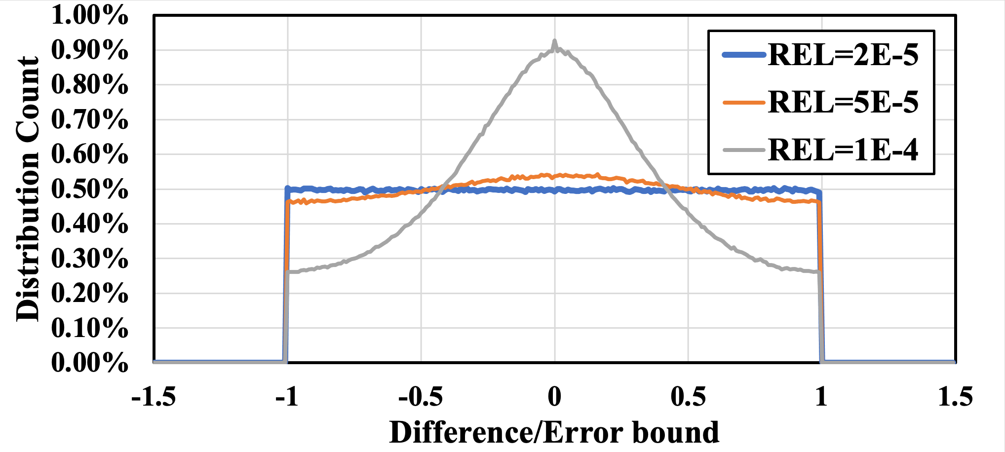
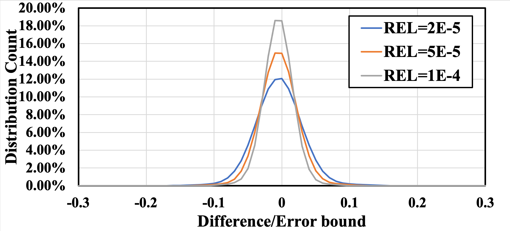
To simulate the compression errors, we have to understand the fault model for a specific compression algorithm. For example, Figure 2 illustrates an example error distribution when compressing and decompressing a typical variable in Nyx cosmology data. It clearly shows that there exists an identifiable error distribution with different compression configurations of the SZ and ZFP compression algorithms. In fact, Lindstrom [14] studied errors distributions of lossy floating-point compressors in a statistical way. The work concludes that lossy compression error distributions depend on their adopted quantization techniques. Specifically, lossy compressors adopted uniform scalar quantization such as SZ [15, 16, 3], SQ [34], and LZ4A [35] tend to generate uniformly distributed errors, while transform-based lossy compressors such as ZFP [17], VAPOR [33], and TTHRESH [32] produce error distributions that are close to normal (a.k.a., Gaussian). Inspired by this work, we mainly focus on these two fault models (i.e., uniform and normal distributions) in this study; however, it is worth noting that LCFI is extensible with any given error distribution (will be described later).
IV Design and Implementation
LCFI111LCFI is publicly available at https://github.com/LCFI/LCFI. is an extension of LLFI[23]. In this Section, we first discuss our design goals and assumptions for LCFI. We then present the improvements and features of LCFI. Finally, we present our implementation details.
IV-A Design Goals and Assumptions
In general, we have four design goals for LCFI as follow:
-
•
Applicability: We aim to create a tool that is simple and easy to use, that users can exploit even without knowing a lot about error-bounded lossy compression. With a simple program written in C/C++, users should be able to easily inject a fault to a specific variable at a specific location. For example, if the target variable is located in a for-loop, the user can inject faults in a specific iteration of this for-loop, which is necessary to change an array’s value.
-
•
Customizable: Given that there are a large number of error distributions in lossy compression (considering future newly designed compressors), it is not feasible to provide a tailored tool for all distributions. We provide a template to users to allow them customize their own error distributions.
-
•
Easy-to-Use: We aim to provide users a simple installation process that does not require editing several setup files. To install LCFI, users only need to edit just one or two YAML-files and run a few commands (e.g., no more than four) to get the injection results. Moreover, LCFI should not require an understanding of how the compiler works or the ability to read IR files.
- •
Additionally, we make the following assumptions about the faults injected by LCFI:
-
•
Faults can only be injected into variables that are on the right of the equal sign due to the nature of LLVM. Changing a variable on the left of the assignment can be achieved by changing all variables on the right of the assignment.
-
•
Faults cannot be injected to the variables located in the main function. This is because most of the faults in the main functions will cause the program to crash, which will make injection meaningless.
-
•
Because LLFI does not support OpenMP, one can only run LCFI on serial programs without multiple threads. In the future, with LLFI-GPU developed, we will further design an OpenMP and CUDA version of LCFI.
IV-B Design of LCFI
Unlike LLFI that focuses on the impact caused by different software faults and hardware faults, LCFI focuses on how different lossy compression errors impact the running of different programs. Thus, to build LCFI, we modify the way LLFI injects faults and faults themselves. The core design of LCFI is shown in Figure 3.
We propose the following designs in LCFI to satisfy the previously described goals. More details will be shown later in Section III.
-
•
Applicability: We provide several YAML files that users can edit. In these YAML files, users can easily select the variable where they want to inject the fault and select what kind of fault model they want to inject. Users are not required to understand how lossy compression works but can still get results directly.
-
•
Customizable: Unlike LLFI’s complex step of customizing faults, we provide a template for the distribution of lossy compression errors. To custom faults or error distributions, users just need to simply edit this template and recompile the code.
-
•
Ease-to-Use: By using the Python scripts that we provide, LCFI can automatically find the location of specific variables in the IR file. Users can use the scripts to notify the injector what index it should target. Thus, users do not need to understand a complicated IR file to use LCFI.
-
•
Top-Down Comprehensive Result: LCFI generates both high-level and underlying results such as standard output files and IR-level results. Users can use both results to perform program-level error propagation analysis.
IV-C LCFI Features
LCFI improves the functionality of LLFI by introducing the following new features:
-
•
Multi-location Unlike LLFI that can inject a fault to only one specific location, LCFI allows to inject a fault at any given location and at any given time.
-
•
For-loop Injection For HPC programs, for-loop is one of the most frequently used loops. For LCFI, we design an interface to set the loop number so that users can inject faults at specific iterations during the for-loop execution. This is imperative if the user wants to inject the fault into an array.
-
•
Custom Distribution We optimize the current LLFI interface to allow users to easily customize their own lossy compression errors.
IV-D Implementation Details
Similar to LLFI, LCFI is implemented using the LLVM-Pass (in C/C++) and Python. We split the LLVM-Pass code and Python code into three modules as follows:
-
•
LLVM-Pass Core is the main module that controls the underlying execution of the target program. It also provides the functionality to trace the execution and insert runtime code.
-
•
Runtime Lib module consists of different fault implementations and determines which variables need to be injected.
-
•
Tools module consists of some useful tools for users to analyze the results from LCFI. It includes Trace_To_Dot, Trace_Union and Trace_Diff.
LCFI results consist of four main outputs as follows:
-
•
Baseline: This output comes from the origin program, which includes golden_std_output, llfi.stat.trace.prof.txt and an output file. golden_std_output is the standard output of the origin program. The llfi.stat.trace.prof.txt records the value changes of every register.
-
•
Program Output: This output comes from the execution of the program with injected faults. If the program does not generate an output file, this part will be empty.
-
•
Error Output: If the program with injected faults crashes, the log will be stored in this output file.
-
•
Standard Output: This file records the execution of the program with injected faults.
-
•
LLFI Stat Output: This file records the value change of every register. If faults have successfully been injected into the program, the injection log will also be stored.
V Usage Model
In this section, we will demonstrate how to customize a distribution of lossy compression errors in LCFI and how to inject the fault into a program written in C/C++. The example C code is shown in LABEL:lst:animate.
In the sample code, the main function calls the process function three times. The process function contains a for-loop that will be executed three times. In each for-loop, the program will print the value in the n array.
After compiling and instrumenting the C code, we will get three IR files. Let us take a look at the demo-lcfi_index.ll first. Listing LABEL:lst:code2 shows its part related to process function. In this file, every IR instruction is given an index so that the injector can recognize different instructions in the next step. We target to inject compression errors on the variable (Line 8 in the example code). To do so, we set variable_name as n and function_name as the process in the configurable YAML file, as shown in Listing LABEL:lst:yaml1. The variable n first appears in Line 8, so we set variable_location as 1. Because n is in a for-loop and is an array, we set the in_arr and in_loop to true. In particular, as we target to inject faults in the 3rd loop, we set loop_num as 3. Running the python script setinput.py generates input.yaml.
Then, let us take a look at demo-lcfi_profiling.ll222This file is generated when trace option is set to true. and demo-lcfi_fi.ll. Both files include some instructions that are used for printing trace information and fault injection. There are some instructions of which trace information is not added in front because these instructions do not return any registers. This kind of instructions always uses the same store opcode because the store instruction only stores some value in a specific register but does not return any registers. That is why assuming that users cannot change the variable on the left of the assignment symbol, as presented in Section • ‣ IV-A.
The next step is profiling and injection. After that, demo-profiling.ll and demo-fi.ll will be compiled to executable files. Then, we can get the results of the baseline program and program with injected faults by executing these executable files. If turning on the trace switch, we can also get trace files for baseline run and run with injected compression faults, similar to Listing LABEL:lst:trace1 and LABEL:lst:trace2. We can use the trace-diff command to analyze the error propagation in terms of program execution. As shown in the listings, the values of index-18 are different, which means ans has been impacted by the compression errors injected to the variable n with the index of 15.
Finally, we can get the outputs of the baseline program and the program with injected faults, as shown in Figure LABEL:lst:results. The values in the third loop are all different from the baseline.
VI Evaluation
In this section, we use different compression fault models (i.e., error distributions) to inject faults into several representative HPC programs. In these programs, we select some typical variables for injection where lossy compression is needed. The names of programs and selected variables are shown in Table I. The goal of our experiment is to demonstrate that LCFI has the ability to inject various compression faults with different error distributions into different program locations.
| Benchmark | Index | Variable Name | Data Type | In Array? | In For-Loop? | Loop Num. |
|---|---|---|---|---|---|---|
| HPCCG [37] | 1469 | x | Double | True | True | 1, 5 |
| Black-Scholes[38] | 40 | xNPrimeofX | Float | False | False | NaN |
| XSBench[39] | 271 | conc | Double | False | True | 2 |
| NPB-MG[40] | 6326 | a1 | Double | False | False | NaN |
VI-A Experimental Configuration
Lossy compression is used for data reduction in HPC applications, thus, we select representative variables with relatively large sizes for fault injection in the core function, as shown in Table I.
-
•
Programs: We use the benchmarks provided by [41], which are very popular HPC benchmarks.
-
•
Index and Variable Name: In the IR format file, a specific llfi-index means a specific variable and its location. Using the index, we can determine the injection location.
-
•
In Loop or Array?: The information of this attribute is discussed in Section V.
-
•
Fault Type: We use four types of fault models which are the combinations of two typical error-bound modes (absolute error and relative error) and two error distributions (uniform distribution and normal distribution).
VI-B Evaluation Results
VI-B1 HPCCG
HPCCG is a simple conjugate gradient benchmark code for a 3D chimney domain. We test the variable x in the waxpby function. We observe that even injecting compression faults on the same variable, different error distributions or locations may lead to different program outputs.
Table II shows the results when injecting faults in the first loop. We observe that every program with faults injected can still converge, but programs injected with absolute errors converge much slower than those with relative errors.
| Fault Type | Relative + Uniform | Relative + Normal | ||||||||
| Error Bound | 1%, 5%, 10%, 50%, 100% | 1%, 5%, 10%, 50%, 100% | ||||||||
| Converge Iter. | 99 (same as baseline) | 99 (same as baseline) | ||||||||
| Fault Type | Absolute + Uniform | Absolute + Normal | ||||||||
| Error Bound | 0.01 | 0.05 | 0.1 | 0.5 | 1 | 0.01 | 0.05 | 0.1 | 0.5 | 1 |
| Converge Iter. | 103 | 103 | 104 | 105 | 105 | 103 | 104 | 105 | 105 | 105 |
Moreover, when we inject faults on variable x in the fifth loop, none of the programs is able to converge within 150 iterations (i.e., the maximum number of iterations set by the program in default). The results are shown in Figure 4. In order to better illustrate the final residual of the program after 150 iterations, we compute a new metric as:
VI-B2 Black-Scholes
Black-Scholes is a program to compute the dynamics of a financial market containing derivative investment instruments. We test the variable xNPrimeofX in the CNDF function. According to the running logs, some of runs are crashed, and others generate corrupted results, none of which are correct. Figure 5 illustrates the percentage of crashed runs and completed (but with corrupted outputs) runs. Due to the paper’s focus (tool development), we will investigate the root cause of these crashes in the future.
| Completed | Crashed | |
|---|---|---|
| Relative Error | 60% | 40% |
| Absolute Error | 50% | 50% |
VI-B3 XSBench
XS-Bench is a mini-app representing a key computational kernel of the Monte Carlo neutron transport algorithm. We test the variable a1 in the calculate_macro_xs function. According to the standard output, although all injected programs can finish the execution, every program with fault injection either generates different output or runs lower with the same output, compared to the baseline program. Listing LABEL:lst:res3 illustrates the different verification checksums generated by the baseline and injected programs. We note that the baseline programs cost about 127 seconds, but the programs with injected faults cost about 260 seconds.
VI-B4 NPB-MG
NPB-MG is a multi-grid (MG) method implemented in the NAS Parallel Benchmarks [40]. In numerical analysis, an MG method is an algorithm for solving differential equations using a hierarchy of discretizations. We test the variable a1 in the vranlc function. We observe that the outputs of all the programs are corrupted with the tested fault types (including error distributions and error-bound modes).
VI-C Observation 1: Corrupted or Not? OR Slow Converge?
According to Section VI-B, we observe that the programs with faults injected can crash (Black-Scholes), generate incorrect results (HPCCG and NPB-MG), or take longer time to complete or converge (HPCCG and XSBench). In addition, some faults may have no impact on the program execution such as HPCCG, which will be discussed in Section VI-D.
Therefore, we can say that our tool can simulate different faulty scenarios and effectively guide users on how to use lossy compressors. As shown in Section VI-B1, we can find that, as the error bound increases, the becomes smaller, which means the final residual becomes larger; in other words, the program converges more slowly. This means that when users try to use lossy compression here, they have to be careful about the error bound to set. As shown in Section VI-B3, even if the simulation time becomes about twice longer, the program with injected fault still cannot get the correct output. This means that users cannot use lossy compression for this specific variable in XSbench.
VI-D Observation 2: Execution Path Changed?
According to Table II, we observe that some injected faults do not have any noticeable impact on the program’s output. We call these faults Benign Faults. Based on the trace file, we find that the fault was injected in the first loop but disappeared in the second loop. The first loop is located in line 5 of Listing LABEL:lst:HPCCG, and the second loop is located in line 7. We get such error propagation figures between benign fault and normal fault333Normal faults are the faults having an impact on the program’s final output., as shown Figure 6. This demonstrates that users can use LCFI to effectively trace lossy compression error propagation.
VII Conclusion and Future Work
In this paper, we propose and develop a new fault injector for lossy compression error called LCFI (Lossy Compression Fault Injector). This tool can realize IR-level analysis for lossy compression errors. LCFI can provide useful insights for developers of lossy compression to design a better compression for specific HPC programs. Based on our evaluation results, we find that different programs have different resilience on lossy compression errors. In specific programs, different variables or even the same variable in different locations may have different sensitivities to a given type of lossy compression error. In the future, we plan to extend LCFI with OpenMP and GPU support, which will have broader prospects and applications.
References
- [1] A. H. Baker, D. M. Hammerling, S. A. Mickelson, H. Xu, M. B. Stolpe, P. Naveau, B. Sanderson, I. Ebert-Uphoff, S. Samarasinghe, F. De Simone, F. Carbone, C. N. Gencarelli, J. M. Dennis, J. E. Kay, and P. Lindstrom, “Evaluating lossy data compression on climate simulation data within a large ensemble,” Geoscientific Model Development, vol. 9, no. 12, 2016.
- [2] A. H. Baker, H. Xu, J. M. Dennis, M. N. Levy, D. Nychka, S. A. Mickelson, J. Edwards, M. Vertenstein, and A. Wegener, “A methodology for evaluating the impact of data compression on climate simulation data,” in Proceedings of the 23rd International Symposium on High-Performance Parallel and Distributed Computing. ACM, 2014, pp. 203–214.
- [3] X. Liang, S. Di, D. Tao, S. Li, S. Li, H. Guo, Z. Chen, and F. Cappello, “Error-controlled lossy compression optimized for high compression ratios of scientific datasets,” in 2018 IEEE International Conference on Big Data. IEEE, 2018, pp. 438–447.
- [4] S. Li, S. Di, X. Liang, Z. Chen, and F. Cappello, “Optimizing lossy compression with adjacent snapshots for n-body simulation data,” in 2018 IEEE International Conference on Big Data. IEEE, 2018, pp. 428–437.
- [5] F. Cappello, S. Di, S. Li, X. Liang, A. M. Gok, D. Tao, C. H. Yoon, X.-C. Wu, Y. Alexeev, and F. T. Chong, “Use cases of lossy compression for floating-point data in scientific data sets,” The International Journal of High Performance Computing Applications, 2019.
- [6] X.-C. Wu, S. Di, F. Cappello, H. Finkel, Y. Alexeev, and F. T. Chong, “Memory-efficient quantum circuit simulation by using lossy data compression,” arXiv preprint arXiv:1811.05630, 2018.
- [7] S. Habib, V. A. Morozov, N. Frontiere, H. Finkel, A. Pope, K. Heitmann, K. Kumaran, V. Vishwanath, T. Peterka, J. A. Insley, D. Daniel, P. K. Fasel, and Z. Lukic, “HACC: extreme scaling and performance across diverse architectures,” Communications of the ACM, vol. 60, no. 1, pp. 97–104, 2016.
- [8] T. E. Fornek, “Advanced photon source upgrade project preliminary design report,” 9 2017.
- [9] L. P. Deutsch, “GZIP file format specification version 4.3,” 1996.
- [10] Zstandard, http://facebook.github.io/zstd/.
- [11] Blosc compressor, http://blosc.org/.
- [12] M. Burtscher and P. Ratanaworabhan, “FPC: A high-speed compressor for double-precision floating-point data,” IEEE Transactions on Computers, vol. 58, no. 1, pp. 18–31, 2008.
- [13] S. W. Son, Z. Chen, W. Hendrix, A. Agrawal, W.-k. Liao, and A. Choudhary, “Data compression for the exascale computing era-survey,” Supercomputing Frontiers and Innovations, vol. 1, no. 2, pp. 76–88, 2014.
- [14] P. Lindstrom, “Error distributions of lossy floating-point compressors,” in Joint Statistical Meetings 2017, 2017.
- [15] S. Di and F. Cappello, “Fast error-bounded lossy hpc data compression with SZ,” in 2016 IEEE International Parallel and Distributed Processing Symposium. IEEE, 2016, pp. 730–739.
- [16] D. Tao, S. Di, Z. Chen, and F. Cappello, “Significantly improving lossy compression for scientific data sets based on multidimensional prediction and error-controlled quantization,” in 2017 IEEE International Parallel and Distributed Processing Symposium. IEEE, 2017, pp. 1129–1139.
- [17] P. Lindstrom, “Fixed-rate compressed floating-point arrays,” IEEE Transactions on Visualization and Computer Graphics, vol. 20, no. 12, pp. 2674–2683, 2014.
- [18] N. Sasaki, K. Sato, T. Endo, and S. Matsuoka, “Exploration of lossy compression for application-level checkpoint/restart,” in 2015 IEEE International Parallel and Distributed Processing Symposium. IEEE, 2015, pp. 914–922.
- [19] J. Calhoun, F. Cappello, L. N. Olson, M. Snir, and W. D. Gropp, “Exploring the feasibility of lossy compression for pde simulations,” The International Journal of High Performance Computing Applications, vol. 33, no. 2, pp. 397–410, 2019.
- [20] T. Reza, J. Calhoun, K. Keipert, S. Di, and F. Cappello, “Analyzing the performance and accuracy of lossy checkpointing on sub-iteration of nwchem,” in 2019 IEEE/ACM 5th International Workshop on Data Analysis and Reduction for Big Scientific Data (DRBSD-5). IEEE, 2019, pp. 23–27.
- [21] P. Lindstrom and M. Isenburg, “Fast and efficient compression of floating-point data,” IEEE Transactions on Visualization and Computer Graphics, vol. 12, no. 5, pp. 1245–1250, 2006.
- [22] G. K. Wallace, “The JPEG still picture compression standard,” IEEE Transactions on Consumer Electronics, vol. 38, no. 1, pp. xviii–xxxiv, 1992.
- [23] Q. Lu, M. Farahani, J. Wei, A. Thomas, and K. Pattabiraman, “Llfi: An intermediate code-level fault injection tool for hardware faults,” in Software Quality, Reliability and Security (QRS), 2015 IEEE International Conference on, Aug 2015, pp. 11–16.
- [24] D. Tao, S. Di, X. Liang, Z. Chen, and F. Cappello, “Improving performance of iterative methods by lossy checkponting,” in Proceedings of the 27th International Symposium on High-Performance Parallel and Distributed Computing. ACM, 2018, pp. 52–65.
- [25] R. D. Evans, L. Liu, and T. M. Aamodt, “Jpeg-act: accelerating deep learning via transform-based lossy compression,” in 2020 ACM/IEEE 47th Annual International Symposium on Computer Architecture (ISCA). IEEE, 2020, pp. 860–873.
- [26] J. Wei, A. Thomas, G. Li, and K. Pattabiraman, “Quantifying the accuracy of high-level fault injection techniques for hardware faults,” in 2014 44th Annual IEEE/IFIP International Conference on Dependable Systems and Networks. IEEE, 2014, pp. 375–382.
- [27] G. Li, K. Pattabiraman, and N. DeBardeleben, “Tensorfi: A configurable fault injector for tensorflow applications,” in 2018 IEEE International Symposium on Software Reliability Engineering Workshops (ISSREW). IEEE, 2018, pp. 313–320.
- [28] A. Poppick, J. Nardi, N. Feldman, A. H. Baker, A. Pinard, and D. M. Hammerling, “A statistical analysis of lossily compressed climate model data,” Computers & Geosciences, vol. 145, p. 104599, 2020.
- [29] S. Li, N. Marsaglia, C. Garth, J. Woodring, J. Clyne, and H. Childs, “Data reduction techniques for simulation, visualization and data analysis,” in Computer Graphics Forum, vol. 37, no. 6. Wiley Online Library, 2018, pp. 422–447.
- [30] P. Lindstrom and M. Isenburg, “Fast and efficient compression of floating-point data,” IEEE Transactions on Visualization and Computer Graphics, vol. 12, no. 5, pp. 1245–1250, 2006.
- [31] M. Ainsworth, O. Tugluk, B. Whitney, and S. Klasky, “Multilevel techniques for compression and reduction of scientific data—the univariate case,” Computing and Visualization in Science, vol. 19, no. 5-6, pp. 65–76, 2018.
- [32] R. Ballester-Ripoll, P. Lindstrom, and R. Pajarola, “TTHRESH: Tensor compression for multidimensional visual data,” IEEE Transactions on Visualization and Computer Graphics, 2019.
- [33] S. Li, S. Jaroszynski, S. Pearse, L. Orf, and J. Clyne, “VAPOR: A visualization package tailored to analyze simulation data in Earth system science,” Atmosphere 2019, vol. 10, no. 488, 2019.
- [34] J. Iverson, C. Kamath, and G. Karypis, “Fast and effective lossy compression algorithms for scientific datasets,” in European Conference on Parallel Processing. Springer, 2012, pp. 843–856.
- [35] J. Kunkel, A. Novikova, E. Betke, and A. Schaare, “Toward decoupling the selection of compression algorithms from quality constraints,” in International Conference on High Performance Computing. Springer, 2017, pp. 3–14.
- [36] G. Li, K. Pattabiraman, S. K. S. Hari, M. Sullivan, and T. Tsai, “Modeling soft-error propagation in programs,” in 2018 48th Annual IEEE/IFIP International Conference on Dependable Systems and Networks (DSN). IEEE, 2018, pp. 27–38.
- [37] HPCCG, https://github.com/Mantevo/HPCCG.
- [38] C. Bienia, S. Kumar, J. P. Singh, and K. Li, “The parsec benchmark suite: Characterization and architectural implications,” in Proceedings of the 17th international conference on Parallel architectures and compilation techniques, 2008, pp. 72–81.
- [39] XSBench, https://github.com/ANL-CESAR/XSBench.
- [40] D. H. Bailey, E. Barszcz, J. T. Barton, D. S. Browning, R. L. Carter, L. Dagum, R. A. Fatoohi, P. O. Frederickson, T. A. Lasinski, R. S. Schreiber et al., “The nas parallel benchmarks,” The International Journal of Supercomputing Applications, vol. 5, no. 3, pp. 63–73, 1991.
- [41] L. Palazzi, G. Li, B. Fang, and K. Pattabiraman, “A tale of two injectors: End-to-end comparison of ir-level and assembly-level fault injection,” in 2019 IEEE 30th International Symposium on Software Reliability Engineering (ISSRE). IEEE, 2019, pp. 151–162.