Metastable soliton necklaces supported by fractional diffraction and competing nonlinearities

Abstract

We demonstrate that fractional cubic-quintic nonlinear Schrödinger equation, characterized by its Lévy index, maintains ring-shaped soliton clusters (“necklaces”) carrying orbital angular momentum. They can be built, in the respective optical setting, as circular chains of fundamental solitons linked by a vortical phase field. We predict semi-analytically that the metastable necklace-shaped clusters persist, corresponding to a local minimum of an effective potential of interaction between adjacent solitons in the cluster. Systematic simulations corroborate that the clusters stay robust over extremely large propagation distances, even in the presence of strong random perturbations.

I Introduction

Ring-shaped soliton clusters, constructed as coherent chains of fundamental solitons, are quasistationary multisoliton bound states. These complexes generalize the concept of necklace-ring beams, which were first studied in self-focusing Kerr media Soljacic-Segev1 ; Soljacic-Segev2 ; Soljacic-Segev3 , and later extended to the nonlinear Schrödinger equation (NLSE) with saturable nonlinearity Desyatnikov-Kivshar1 .

Usually, many-soliton circular structures tend to destroy themselves through expansion or collapse, an experimentally relevant issue being how to maintain their quasi-stationary propagation. To balance the destructive trends, a vortical phase profile can be imposed onto the clusters Desyatnikov-Kivshar2 . In this context, various nonlinearities, including saturable Desyatnikov-Kivshar3 , competing quadratic-cubic Kartashov-Cra-Mih-Torner , cubic-quintic Mihalache-PRE68-046612 , and nonlocal Buccoliero-PRL-98-053901 , were employed to enhance the robustness of the circular soliton clusters. It was also demonstrated that two-dimensional (2D) soliton clusters can be supported in active systems, such as pumped nonlinear optical cavities Vladimirov-Skryabin-PRE65-046606 ; Skryabin-Vladimirov-PRL89-044101 . A possibility of the existence of 3D soliton clusters, composed of spatiotemporal optical solitons, has also been explored Perez-Garcia-Vekslerchik ; Crasovan-PRE67-046610 ; Mihalache-JOB-6-S333 . Creation of necklace beams was experimentally demonstrated in photorefractive Desyatnikov-JOSAB-19-586 , nonlocal Rotschild-OL-31-3312 , and Kerr Grow-PRL99-133902 media. More recently, assemblage of metastable necklace clusters of 2D “quantum droplets” was predicted Kartashov-Malomed-Torner in the framework of the Gross-Pitaevskii equations with the cubic nonlinearity modified by the logarithmic factor, which is induced by the Lee-Huang-Yang correction to the mean-field dynamics of Bose-Einstein condensates (BEC) AstraPetrov . Further exploration of physically relevant settings which maintain necklace complexes in a quasi-stable form remains a relevant objective for theoretical and experimental work. In particular, the creation of nearly stable necklace patterns with imprinted overall vorticity in a medium with the cubic-quintic (CQ) nonlinearity (liquid carbon disulfide) was very recently reported in Ref. Albert .

In this connection, it is relevant to stress that the vortical soliton clusters and usual axisymmetric vortex solitons Michinel ; Pego ; PhysD ; LPF-Mal-Mih2 are different types of beams carrying the orbital angular momentum (OAM). The clusters carry OAM in the explicit form, being rotating azimuthally modulated necklace-like structures, while the vortex solitons carry OAM in the “hidden” form, being axisymmetric structures, while OAM is stored in their phase circulation. Circular soliton clusters, considered in the present work, are constructed as quasi-steady states, realizing local minima of an effective potential. Vortex solitons are fully stationary modes with a topological charge, s, representing the vorticity. Accordingly, stable vortex solitons keep their shape in the course of the propagation, while unstable ones are broken up by azimuthal perturbations in several fragments, whose number is usually (s+1). On the other hand, the circular clusters (“necklaces” ) should be created differently, as they do not emerge as result of the splitting of unstable vortex solitons. In particular, the number of separate elements (“beads” ) in the necklace is independent of s. Unlike the uniform vortex modes with the “hidden” vorticity, for clusters their steadiness is a major issue.

Theoretical studies of optical solitons in NLSE models were lately extended in two noteworthy directions. On the one hand, the theory has been expanded for non-Hermitian optical systems, which are modeled by NLSEs with parity-time-symmetric complex potentials, see reviews. RMP-PT-88-035002 ; Suchkov ; Feng ; El-Ganainy and an experimental report Peschel . On the other hand, much interest has been drawn to the fractional Schrödinger equations (FSEs), which were originally proposed by Laskin Laskin1 ; Laskin2 ; Laskin3 and, in a rigorous mathematical form, by Hu and Kallianpur Hu . In the quantum theory, FSE was derived Laskin1 as a model in which the consideration of Feynman path integrals over Brownian trajectories leads to the standard Schrödinger equation, while path integrals over “ skipping” Lévy trajectories lead to the FSE Laskin2 . Experimental schemes have been proposed for realization of FSE in condensed-matter settings FSE11 ; excitons and in optical media FSE12 , where the effective fractional diffraction may be realized in cavities including optical filters and phase masks early1 ; early2 . Actually, optical cavities offer a testbed to explore the propagation dynamics and eigenmodes of optical beams governed by linear and nonlinear FSEs. Following this approach, many noteworthy properties have been revealed in the framework of FSE FSE13 ; FSE14 ; FSE15 ; FSE16 ; FSE17 ; FSE18 ; FSE19 ; FSE20 ; FSE21 ; FSE22 ; FSE23 ; FSE24 ; FSE25 . Adding nonlinear terms to FSE NLFSE1 ; NLFSE2 , recent publications have predicted a variety of fractional solitons NLFSE3 ; NLFSE4 ; NLFSE5 ; NLFSE6 ; NLFSE7 ; NLFSE8 ; NLFSE9 ; NLFSE10 ; NLFSE11 ; NLFSE12 ; NLFSE13 ; NLFSE14 ; NLFSE15 ; NLFSE16 ; NLFSE17 ; NLFSE18 ; NLFSE19 ; NLFSE20 ; NLFSE21 ; LPF-Mal-Mih1 ; CQDai ; Zeng ; Yingji_latest ; LPF-Mal-Mih2 .

In this work, we aim to construct circular soliton clusters in the model combining fractional diffraction and competing CQ nonlinear terms. The paper is organized as follows. The model, including a discussion of its implementation in optics, and numerically found fundamental solitons, is introduced in Sec. II, which is followed by identification of an effective potential energy of the interaction between adjacent solitons, and construction of necklace-shaped soliton clusters, in a semi-analytical form, in Sec. III. Robust propagation of metastable soliton clusters under the action of perturbations is additionally reported, by means of systematic numerical simulations, in Sec. IV. The paper is concluded by Sec. V.

II The model and fundamental solitons

We consider beam propagation along the $z$-axis in a nonlinear isotropic medium with the CQ nonlinear correction to the refractive index, $n_{\mathrm{nonlin}}(I)=n_{2}I-n_{4}I^{2}$, where $I$ is the light intensity, $n_{2}$ and $n_{4}$ being coefficients accounting, respectively, for the cubic self-focusing and quintic defocusing. The respective fractional NLSE, with propagation distance $z$ and transverse coordinates $\left(x,y\right)$, is

$$2ik_{0}\frac{\partial A}{\partial z}-\left(-\nabla_{\perp}^{2}\right)^{\alpha/2}A+\frac{2k_{0}^{2}}{n_{0}}n_{\mathrm{nonlin}}A=0,$$ (1)

where $A(z,x,y)$ is the local amplitude of the optical field, the intensity being $I\equiv|A|^{2}$, $k_{0}=2\pi n_{0}/\lambda$ is the wavenumber, which is determined by carrier wavelength $\lambda$, and $n_{0}$ is the background refractive index. The fractional-diffraction operator in Eq. (1), with the corresponding Lévy index $\alpha$, belonging to interval $1\leq\alpha\leq 2$, is defined as

$$\left(-\nabla_{\perp}^{2}\right)^{\alpha/2}A\left(x,y\right)=\mathcal{F}^{-1}\left[\left(k_{x}^{2}+k_{y}^{2}\right)^{\alpha/2}\mathcal{F}A(x,y)\right],$$ (2)

JMP51-062102 ; JMP54-012111 ; CMA71 , where $\mathcal{F}$ and $\mathcal{F}^{-1}$ are operators of the direct and inverse Fourier transform, $k_{x,y}$ being wavenumbers conjugate to transverse coordinates $\left(x,y\right)$. By means of rescaling, $\Psi(\zeta,\xi,\eta)=\sqrt{n_{4}/n_{2}}A(z,x,y)$, $\zeta=\left(k_{0}n_{2}^{2}/n_{0}n_{4}\right)z$, and $\left(\xi,\eta\right)=\left(2k_{0}^{2}n_{2}^{2}/n_{0}n_{4}\right)^{1/\alpha}\left(x,y\right)$, Eq. (1) is cast in the normalized form,

$$i\frac{\partial\Psi}{\partial\zeta}-\left(-\nabla_{\perp}^{2}\right)^{\alpha/2}\Psi+\left|\Psi\right|^{2}\Psi-\left|\Psi\right|^{4}\Psi=0.$$ (3)

Equation (1) with $\alpha\leq 1$ and cubic-only self-focusing gives rise to the wave collapse NLFSE21 , which destabilizes solitons; however, the quintic self-defocusing term suppresses the instability and makes it possible to construct stable soliton states for $\alpha\leq 1$ as well LPF-Mal-Mih1 .

In the linear limit, Eq. (3) models the free transmission of optical beams under the action of fractional diffraction. Experimental setups which realize this propagation regime were proposed in Refs. FSE12 and FSE14 . In particular, the former setting is designed as a Fabry-Perot resonator, with two convex lenses and two phase masks inserted into it. The first lens converts the input beam into the Fourier (dual) space, then a central phase mask, whose position defines the position of the system’s Fourier plane, performs the transformation of the beam in the dual space, as per Eq. (2), and, eventually, the second lens converts the output beam back from the dual domain into the real (coordinate) one. Thus, the fractional diffraction is effectively executed in the Fourier representation of the field amplitude, and the linear version of Eq. (3) governs the circulation of the beam in the cavity, averaged over many cycles. As a result, the linearized version of Eq. (3) gives rise to conical diffraction of 1D and 2D input Gaussian beams FSE14 ; FSE19 .

The usual cubic nonlinearity can be incorporated in the setup by inserting a piece of a Kerr material in the cavity. To maintain the effectively local form of the nonlinearity, the material should be inserted between an edge mirror and the lens closest to it, where the beam’s propagation takes place in the spatial domain (rather than in the dual one). The CQ terms may be similarly induced by a sample of an optical material combining the self-focusing and defocusing cubic and quintic nonlinearities, whose absorption is low enough to be neglected. This may be, as mentioned above, carbon disulfide in the liquid form, which was used for the creation of stable (2+1)-dimensional spatial solitons PRL110-013901 , quasi-stable (2+1)-dimensional optical solitons with embedded vorticity PRA93-013840 , and, very recently, of quasi-stable necklace arrays of optical beams with imprinted vorticity Albert . Another appropriate CQ material is a colloidal suspension of metallic nanoparticles, in which strengths of cubic and quintic nonlinearities may be accurately adjusted by selecting the size and concentration of the particles Cid .

Proceeding to the consideration of the full nonlinear equation (3), we first address stationary solutions with a real propagation constant, $\beta$:

$$\Psi\left(\zeta,\xi,\eta\right)=\psi\left(\xi,\eta\right)e^{i\beta\zeta},$$ (4)

where complex function $\psi(\xi,\eta)$ obeys the equation

$$-\left(-\nabla_{\perp}^{2}\right)^{\alpha/2}\psi+\left|\psi\right|^{2}\psi-\left|\psi\right|^{4}\psi-\beta\psi=0.$$ (5)

Further, the complex function is substituted in the Madelung’s form, $\psi(\xi,\eta)=U(\xi,\eta)e^{i\phi(\xi,\eta)}$, with real amplitude $U(\xi,\eta)$ and phase $\phi(\xi,\eta)$. In polar coordinates $(r,\theta)$, related to the underlying Cartesian coordinates as usual, $\xi=r\cos\theta$, $\eta=r\sin\theta$, soliton solutions to Eq. (3) with integer embedded vorticity $s$ are looked for as LPF-Mal-Mih2

$$\psi(r,\theta)=U(r)e^{is\theta}.$$ (6)

The self-trapped fundamental states, with $s=0$, are known as Townes solitons of the conventional 2D NLSE with the cubic-only term. In 1D, exact fundamental solitons of the equation with the quintic-only self-focusing term also play the role of solitons of the Townes type Salerno ; Shamriz . These solitons are unstable because the same equations admit the critical collapse Fibich . In the case of the CQ nonlinearity, the fundamental solitons, in 2D and 1D settings alike, realize the system’s ground state (which is missing in the presence of the collapse).

The self-trapping of the solitons implies that $U(r)$ exponentially decays at $r\rightarrow\infty$. Using the same argument as recently applied to the FSE with operator $\left(-\partial^{2}/\partial x^{2}\right)^{\alpha/2}$ NLFSE21 , viz., the consideration of the variation of the integral expression, which defines the nonlocal operator (2), with respect to rescaling of coordinates $x$ and $y$, it is straightforward to conclude that a general form of the exponentially decaying tails of the soliton is

$$U(r)\propto\exp\left[-\left(\frac{2}{C_{\alpha}}\beta\right)^{1/\alpha}r\right],$$ (7)

where the positive constant $C_{\alpha}$ is not universal, except for $C_{\alpha=2}=1$. Note also that the proportionality multiplier, dropped in Eq. (7), includes a power-law pre-exponential factor $\sim r^{-\gamma_{\alpha}}$ with some constant $\gamma_{\alpha}>0$ (obviously, $\gamma_{\alpha=2}=1/2$).

The power (alias integral norm) and $z$-component of the angular momentum of the vortex are

$$P=\iint\left|\psi\left(\xi,\eta\right)\right|^{2}d\xi d\eta,$$ (8)

$$L_{z}=\frac{\mathbf{e}_{z}}{2i}\cdot\iint\mathbf{\rho}\times\left(\psi^{\ast}\nabla\psi-\psi\nabla\psi^{\ast}\right)d\xi d\eta,$$ (9)

where $\mathbf{\rho}=\left(\xi,\eta\right)$ is the vector of the integration coordinates, and $\mathbf{e}_{z}$ is a unit vector in the propagation direction. The Hamiltonian of Eq. (3) is

$$H=\iint\left[\Psi^{\ast}\left(-\nabla_{\perp}^{2}\right)^{\alpha/2}\Psi-\frac{1}{2}\left|\Psi\right|^{4}+\frac{1}{3}\left|\Psi\right|^{6}\right]d\xi d\eta.$$ (10)

Note that, with regard to the definition given by Eq. (2), expression (10) produces a real Hamiltonian Laskin1 .

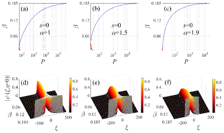
Figure 1: The propagation constant of the fundamental solitons (with $s=0$) versus their integral power (shown on the logarithmic scale), for different values of the Lévy index: (a) $\alpha=1$; (b) $\alpha=1.5$; (c) $\alpha=1.9$. Thin blue and thick red curves denote stable and unstable solutions, respectively. Profiles of the cross-section, $\left|\psi\left(\xi,\eta=0\right)\right|$, of the fundamental solitons for the propagation constant taking values $0.006\leq\beta\leq 0.185$, with step $\Delta\beta=0.001$, are depicted in panels (d) for $\alpha=1$, (e) for $\alpha=1.5$, and (f) for $\alpha=1.9$.

Families of fundamental solitons with different values of the Lévy index $\alpha$ were numerically generated by dint of the Newton-conjugate-gradient method NCG ; Book1 . We display dependences of their propagation constant $\beta$ on power $P$ for different values of the Lévy index in Fig. 1. It is seen that two branches of the $\beta(P)$ curves merge at points with the vertical tangent, $d\beta/dP=0$. Top ($d\beta/dP>0$) and bottom ($d\beta/dP<0$) branches are, severally, stable and unstable, as established below by the linear-stability analysis and direct simulations. These conclusions are correctly predicted by the celebrated Vakhitov-Kolokolov criterion VK ; Fibich . Note that this criterion is irrelevant for the stability of vortex solitons with $s\geq 1$ against azimuthal instabilities that may split the ring-shaped vortex modes LPF-Mal-Mih2 . The point with $d\beta/dP=0$ corresponds to a threshold (minimum) value of the total power, $P_{\mathrm{th}}^{(s=0)}$, necessary for the existence of the fundamental solitons. In the cases shown in Fig. 1 the numerically found threshold values for the fundamental solitons are $P_{\mathrm{th}}^{(s=0)}(\beta=0.016)|_{\alpha=1}\approx 61.764$, $P_{\mathrm{th}}^{(s=0)}(\beta=0.03)|_{\alpha=1.5}\approx 24.734$, and $P_{\mathrm{th}}^{(s=0)}(\beta=0.011)|_{\alpha=1.9}\approx 14.271$. Further, the cross-section profiles of the fundamental solitons, in the form of $\left|\psi\left(\xi,\eta=0\right)\right|$, are displayed in Figs. 1(d-f), for propagation constants $\beta$ ranging from $0.006$ to $0.185$. As is common for models with competing nonlinearities, the solitons develop a flat-top shape in the limit of large powers.

The goal of this paper is to construct soliton clusters composed of fundamental solitons in free space (without an external potential). Before constructing the clusters, the stability of the fundamental solitons needs to be established, which can be done in the framework of the linearization of Eq. (3) for small perturbations. To this end, we searched for the perturbed solutions of Eq. (3) in a form

$$\Psi\left(\xi,\eta,\zeta\right)=e^{i\beta\zeta}\left[\psi\left(\xi,\eta\right)+\epsilon u\left(\xi,\eta\right)e^{\delta\zeta}+\epsilon v^{\ast}\left(\xi,\eta\right)e^{\delta^{\ast}\zeta}\right],$$ (11)

where $\psi$ is the stationary solution with propagation constant $\beta$ defined as per Eq. (4), the asterisk stands for the complex conjugation, while $u\left(\xi,\eta\right)$ and $v\left(\xi,\eta\right)$ are complex eigenmodes of perturbations, with an infinitesimal amplitude $\epsilon$ Birnbaum . Further, $\delta\equiv\delta_{R}+i\delta_{I}$ is a complex eigenvalue of Eq. (12), $\delta_{R}$ being the linear-instability growth rate. Obviously, the stability condition amounts to $\delta_{R}=0$, for all eigenvalues.

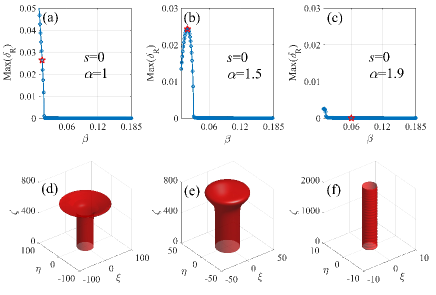
Figure 2: Panels (a), (b), and (c) show the largest linear instability growth rate of the fundamental-soliton families from Figs. 1(a-c). Results of direct simulations of the evolution of particular fundamental solitons, marked by red stars in the top row, are displayed by isosurfaces drawn at a constant-intensity level, $\left|\Psi\right|^{2}=0.05$ in panels (d,e), and $\left|\Psi\right|^{2}=0.50$ in (f). Panel (d): an unstable fundamental soliton, with $\alpha=1$ and $\beta=0.012$; (e) an unstable one, with $\alpha=1.5$ and $\beta=0.018$; (f) a stable fundamental soliton with $\alpha=1.9$ and $\beta=0.06$.

The substitution of expression (11) in Eq. (3) and subsequent linearization leads to the following eigenvalue problem:

$$i\left(\begin{array}[]{cc}\mathit{L}_{11}&\mathit{L}_{12}\\ -\mathit{L}_{12}^{\ast}&-\mathit{L}_{11}^{\ast}\end{array}\right)\left(\begin{array}[]{c}u\\ v\end{array}\right)=\delta\left(\begin{array}[]{c}u\\ v\end{array}\right),$$ (12)

with matrix elements $\mathit{L}_{11}=-\left(-\nabla_{\perp}^{2}\right)^{\alpha/2}+2\left|\psi\right|^{2}-3\left|\psi\right|^{4}-\beta$ and $\mathit{L}_{12}=\psi^{2}+2\left|\psi\right|^{2}\psi^{2}$. In the context of BEC, linearized equations for small perturbations are usually called Bogoliubov-de Gennes equations Pit . Note that the choice of the ansatz for the perturbed solution in the form of Eq. (11), with the combination of amplitudes $u$ and $v^{\ast}$, is convenient because it leads to Eq. (12) for two-component eigenfunctions which does not include complex conjugation.

The linear problem based on Eq. (12) was solved by means of the Newton-conjugate-gradient method NCG ; Book1 . Differently from the conventional NLSE with the CQ nonlinearity, corresponding to $\alpha=2$ in Eq. (1), in which the fundamental solitons are completely stable Pego , the fundamental solitons are found to be unstable in intervals $0.006<\beta\leq 0.016$ (for $\alpha=1$), see Fig. 2(a), $0.006<\beta\leq 0.030$ (for $\alpha=1.5$) in Fig. 2(b), and $0.006<\beta\leq 0.011$ (for $\alpha=1.9$) in Fig. 2(c). These results corroborate that the fundamental-soliton branches with a negative slope, $d\beta/dP<0$, are linearly unstable, while the positive-slope ones are stable, i.e., the stability of the fundamental solitons fully complies with the Vakhitov-Kolokolov criterion. In Figs. 2(d) and 2(e), the results of direct simulations demonstrate that unstable fundamental solitons at first keep their integrity, and then start to spread out, see also movies Visualization 1 and Visualization 2 in Supplemental Material. In Fig. 2(f), a linearly-stable fundamental soliton robustly propagates, under the action of random perturbations with a $5\%$ relative amplitude, over the distance of $\zeta=2000$, which is tantamount to $\sim 50$ diffraction lengths of this soliton.

III The interaction energy and construction of soliton clusters

The necklace-shaped soliton cluster of radius $R$ is constructed as a superposition of $N$ identical fundamental solitons with a superimposed phase distribution carrying the integer global vorticity $M$. Thus, the initial field distribution is set as

$$\Psi\left(\zeta=0\right)=\exp\left(iM\theta\right)\sum\limits_{n=1}^{N}U_{0}(\left|\mathbf{r}-\mathbf{r}_{n}\right|),$$ (13)

where $U_{0}$ is a stable fundamental soliton, and $\mathbf{r}_{n}=\{R\cos(2\pi n/N),R\sin(2\pi n/N)\}$ is the position of the center of the $n$-th soliton in the cluster. The evolution of the pattern is governed by interaction forces between adjacent solitons, which, in turn, depend on the phase shift and separation between them. Note that ansatz (13) includes a linear phase distribution with respect to the angular coordinate, $\theta$, rather than a staircase phase structure, because the former one is more likely to form a quasi-stable structure Crasovan-PRE67-046610 .

As concerns the input necessary for the creation of soliton clusters introduced in the form of Eq. (13), in the experiment it can be put together as a set of several parallel beams placed along the ring, while a vortex phase plate may be used to imprint the phase pattern, which represents the overall vorticity [$M$ in Eq. (13)], onto the multi-beam cluster.

Here, we emphasize the difference of physical properties between the vortex soliton and necklace-shaped soliton cluster. Vortex solitons in Ref. LPF-Mal-Mih2 are stationary solutions of Eq. (3), which may be stable or unstable. However, necklace-shaped soliton clusters, discussed in this paper, are not stationary solutions of Eq. (3). They are composed of stable fundamental solitons of Eq. (3), placed along a ring. While Eq. (3) produces no completely stable necklace-shaped soliton clusters, they can be found in a quasi-stable form. Their existence is predicted by minimization of the effective potential of interaction between adjacent solitons in the cluster, cf. Ref. Kartashov-Malomed-Torner .

Since the necklace may be considered as an azimuthally modulated vortex soliton, one may expect that necklace clusters can be maintained by Eq. (3) if their integral power exceeds the known threshold value, $P_{\mathrm{th}}^{(s=1)}$ LPF-Mal-Mih2 , above which this equation gives rise to stable vortex solitons. This circumstance is elaborated below, see Eq. (16).

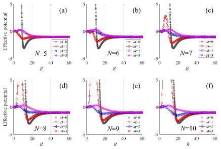
Figure 3: The effective potential given by ansatz (13), numerically computed as per Eq. (15), with different values of vorticity $M$ and number of individual fundamental solitons, $N$, vs. the cluster’s radius, $R$, for (a) $N=5$, (b) $N=6$, (c) $N=7$, (d) $N=8$, (e) $N=9$, and (f) $N=10$. Here, the Lévy index is $\alpha=1.5$, and the integral power of each individual soliton is fixed to be $P_{\mathrm{sol}}=84.1$.

	$N=5$	$N=6$	$N=7$	$N=8$	$N=9$	$N=10$
$M=0$	$11.25$	$13.05$	$14.90$	$16.85$	$18.80$	$20.75$
$M=1$	$10.35$	$11.90$	$13.85$	$15.90$	$17.95$	$20.00$

Table 1: The values of $R_{\min}$, at which the effective potential (15) of the necklace-cluster ansatz (13), with vorticities $M=0$ and $1$, attains a minimum, for different numbers $N$ of individual fundamental solitons in the ansatz, see Fig. 3.

The force of the interaction between fundamental solitons with phase difference $\chi$, separated by large distance $L$, is determined by an effective interaction potential, which is determined by the integral of overlapping between an exponentially decaying tail of each soliton and the core of its mate. Taking into regard the general asymptotic form of the tails, given by Eq. (7), we conclude that the potential of the soliton-soliton interaction may be estimated, as per Ref. 1998 , as

$$W(L)\simeq-W_{0}\cos\chi\cdot\exp\left[-\left(\frac{2}{C_{\alpha}}\beta\right)^{1/\alpha}L\right],$$ (14)

where $W_{0}$ is a positive factor, which may be a slowly decaying function of $L$ (for $\alpha=2$, $W_{0}=\mathrm{const}\cdot L^{-1/2}$), while factor $\cos\chi$ is a universal one 1998 . For the ansatz defined by Eq. (13), one has $L=2R\sin\left(\pi/N\right)$, $\chi=2\pi M/N$.

For the whole necklace cluster, the scaled potential, normalized to the energy of the same set of infinitely separated (non-interacting) solitons, may be defined as

$$\mathrm{Effective~{}potential}=H(R)/H(R\rightarrow\infty),$$ (15)

where $H$ is the full Hamiltonian (10). It can be computed numerically as a function of $R$ for given vorticity $M$ and number of individual “ bids in the necklace” , i.e., individual fundamental solitons, $N$, by substituting ansatz (13) in integral expression (10).

First, we address the case of $\alpha=1.5$. In this case, Eq. (3) maintains stable solitons with vorticity $s=1$ if the integral power exceeds the above-mentioned threshold value, $P_{\mathrm{th}}^{(s=1)}\approx 383$, see Table 1 in Ref. LPF-Mal-Mih2 . Therefore, a set of fundamental solitons, each taken (for instance) with $P_{\mathrm{sol}}=84.1$ and $\beta=0.12$, may have a chance to build robust clusters with $M=1$ and

$$N>P_{\mathrm{th}}^{(s=1)}/P_{\mathrm{sol}}\approx 4.6,$$ (16)

which actually implies $N\geq 5$.

In Fig. 3, the dependence of the effective potential (15) on the cluster’s radius $R$ is presented for different integer values of $M$ and $N$. These results reveal that the necklace clusters with vorticities $M=0$ and $1$ exhibit visible local minima of the interaction potential at a specific value of the cluster’s radius, $R_{\min}$. These numerically identified values for $M=0$ and $1$ are summarized in Table 1 for different numbers of solitons in the cluster, $N$. The results demonstrate that $R_{\min}$ increases with the increase of $N$. For the clusters with $M=2$, local energy minima are observed in Figs. 3(e,f) for $N=9$ and $10$, but, according to data from Table 1 in Ref. LPF-Mal-Mih2 , the respective values of the total power of initial cluster (13) are lower than the corresponding stability-threshold value for the axisymmetric vortex soliton, cf. Eq. (16). Therefore, the minima of the potential energy for $M=2$ cannot produce stable necklace patterns. Lastly, Fig. 3 does not produce local energy minima for the clusters with $M=3$.

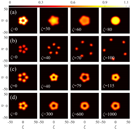
Figure 4: Different scenarios of the evolution of initial necklace soliton clusters (13), built of $N=5$ fundamental solitons at $\alpha=1.5$ (in the absence of random perturbations). (a) Gradual fusion into a large fundamental soliton with initial mean angular velocity $\omega_{0}=$ $0$ [given by Eq. (18) at $\zeta=0$], at $M=0$, $R=11.25$. (b) Expansion and rotation for $M=2$, $R=10.35$, and $\omega_{0}=$ $0.0128$. (c) Periodic oscillations and rotation for $M=1$, $R=13$, and $\omega_{0}=$ $0.005$. (d) Propagation of the rotating cluster with a nearly constant radius, for $M=1$, $R=10.35$, and $\omega_{0}=$ $0.0071$. Local intensity $\left|\Psi\right|^{2}$ is shown at different values of propagation distances $\zeta$, which correspond to red circles in the $R(\zeta)$ dependences in the top row of Fig. 5.

To check the predictions produced by the effective potential, we numerically simulated the propagation of the necklace clusters built of $N=5$ fundamental solitons [see Fig. 3(a)] by means of the split-step Fourier method. In the course of the simulations, the evolution of the cluster’s mean radius $R\left(\zeta\right)$, mean angular velocity $\omega\left(\zeta\right)$, and depth of the azimuthal modulation $\Theta\left(\zeta\right)$ was monitored. These quantities were defined as follows:

$$R\left(\zeta\right)\equiv P^{-1}\iint\sqrt{\xi^{2}+\eta^{2}}\left|\psi\left(\xi,\eta\right)\right|^{2}d\xi d\eta,$$ (17)

$$\omega\left(\zeta\right)\equiv L_{z}/I,I\equiv\iint\left(\xi^{2}+\eta^{2}\right)\left|\psi\left(\xi,\eta\right)\right|^{2}d\xi d\eta,\omega_{0}=\omega\left(\zeta=0\right),$$ (18)

and

$$\Theta\left(\zeta\right)\equiv\frac{\left|\Psi\right|_{\max}^{2}-\left|\Psi\right|_{\min}^{2}}{\left|\Psi\right|_{\max}^{2}+\left|\Psi\right|_{\min}^{2}},$$ (19)

where $\left|\Psi\right|_{\max}^{2}$ and $\left|\Psi\right|_{\min}^{2}$ are the maximum and minimum values of $\left|\Psi\right|^{2}$, as functions of $\theta$, along the circumference at which the solution has a radial maximum in each cluster’s configuration.

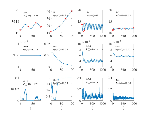
Figure 5: The evolution of the cluster’s mean radius (top row), mean angular velocity (middle row), and depth of the azimuthal modulation (bottom row), which are defined as per Eqs. (17), (18), and (19), respectively. The columns, from left to write, correspond, respectively, to rows (a) – (d) in Fig. 4.

Results produced by the simulations are presented in Fig. 4. For $M=0$, interactions between adjacent fundamental solitons are attractive, according to Eq. (14), therefore the multi-soliton cluster fuses into a fundamental state, as shown in the top row of Fig. 4, even for the initial radius taken as $R=R_{\min}$. On the other hand, for $M=2$, the soliton-soliton interactions, with $\chi=\pi$, are repulsive, thus giving rise to a resulting repulsive force acting on each individual soliton in the radial direction. For this reason, the effective potential energy (15) has no local minimum in this case, see Fig. 3(a). As a result, the cluster expands and rotates, as seen in Fig. 4(b). For $M=1$, i.e., $\chi=3\pi/5$, the interaction potential (14) is weakly attractive, but the net angular momentum of the circular cluster prevents fusion into an axisymmetric vortex soliton. In this case, the cluster with initial radius $R>R_{\min}$ performs quasiperiodic cycles of expansion and shrinkage (in combination with rotation), as shown in Fig. 4(c). The most essential finding is that the cluster with initial radius $R\approx R_{\min}$ gives rise a quasi-stationary state, which performs persistent rotation with minimal radial oscillations, see Fig. 4(d). This mechanism of the effective stabilization of the rotating necklace cluster is somewhat similar to that recently reported in the framework of the usual 2D NLSE with the nonlinearity corresponding to quantum droplets Kartashov-Malomed-Torner . In Fig. 5, the evolution of the cluster’s mean radius, cluster’s mean angular velocity, and depth of the azimuthal modulation is monitored, to display further details of the variation of the cluster’s structure and rotational speed in the course of the propagations. The first panel in the middle row of Fig. 5 shows the case of the cluster’s mean angular velocity equal to zero, therefore it does not rotate. In the second panel in the middle row of Fig. 5, the cluster exhibits rotation with a decreasing angular velocity. In the last two panels in the middle row of Fig. 5, the cluster’s mean angular velocity fluctuates around non-decaying mean values, which indicates that the respective clusters perform persistent rotation with small radial oscillations in the transverse plane.

IV Robust propagation of metastable soliton clusters under the action of perturbations

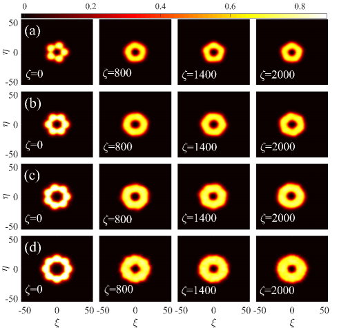
Figure 6: Typical examples of the metastable propagation of the rotating necklace-shaped soliton clusters built of $N$ fundamental solitons, with Lévy index $\alpha=1.5$, initial radius $R=R_{\min}$, and superimposed vorticity $M=1$, in the presence of random perturbations produced by factor (20): (a) $N=5$, $R=10.35$, and $\omega_{0}=$ $0.0071$, (b) $N=6$, $R=11.9$, and $\omega_{0}=$ $0.0058$, (c) $N=7$, $R=13.85$, and $\omega_{0}=$ $0.0044$, (d) $N=8$, $R=15.9$, and $\omega_{0}=$ $0.0036$. The local intensity $\left|\Psi\right|^{2}$ is shown at different values of propagation distances $\zeta$, which correspond to red circles in the $R(\zeta)$ dependences in the top row of Fig. 7.

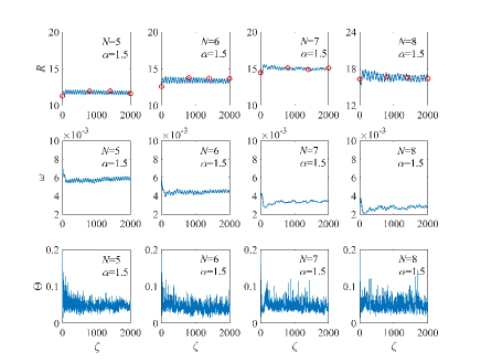
Figure 7: The evolution of the cluster’s mean radius (top row), mean angular velocity (middle row), and depth of the azimuthal modulation (bottom row), which are defined as per Eqs. (17), (18), and (19), respectively. The columns, from left to write, correspond, respectively, to rows (a) – (d) in Fig. 6.

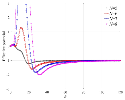
Figure 8: The effective potential energy of the soliton clusters, composed of $N$ fundamental solitons, with superimposed vorticity $M=1$, defined as per Eq. (15), vs. the cluster’s radius $R$: (a) $N=5$, (b) $N=6$, (c) $N=7$, (d) $N=8$. In this case, the Lévy index is $\alpha=1$, and the integral power of all clusters is $P=332.35$.

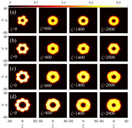
Figure 9: Metastable propagation of the rotating soliton clusters with Lévy index $\alpha=1$, initial radius $R=R_{\min}$, and vorticity $M=1$, in the presence of random perturbations imposed by factor (20): (a) $N=5$, $R=19.8$, and $\omega_{0}=$ $0.002$, (b) $N=6$, $R=23.55$, and $\omega_{0}=$ $0.0015$, (c) $N=7$, $R=27.6$, and $\omega_{0}=$ $0.0012$, (d) $N=8$, $R=31.6$, and $\omega_{0}=$ $0.001$. The local intensity $\left|\Psi\right|^{2}$ is shown at different values of propagation distance $\zeta$ that correspond to red circles in the top row of Fig. 10.

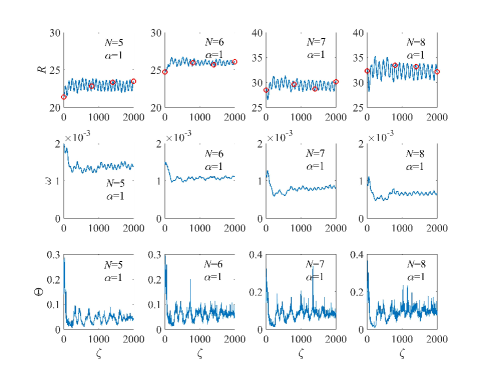
Figure 10: The evolution of the cluster’s mean radius (top row), mean angular velocity (middle row), and depth of the azimuthal modulation (bottom row) for different number of fundamental solitons $N$ in Fig. 9. The columns, from left to write, correspond, respectively, to rows (a) – (d) in Fig. 9.

To further elucidate the robustness of the soliton clusters with the properly chosen initial radius, $R=R_{\min}$, we added random perturbation to the initial profiles of the soliton cluster in Eq. (13), multiplying it by

$$\mathrm{perturbing~{}factor}=[1+0.1(\rho_{1}+i\rho_{2})],$$ (20)

where $\rho_{1}$ and $\rho_{2}$ are uniformly distributed random numbers in the interval of $[-0.5,0.5]$. In Fig. 6, the simulations demonstrate that the rotating necklace clusters, composed of different numbers of fundamental solitons ($N=5,6,7$, and $8$), with initial radius $R=R_{\min}$, can survive, as metastable patterns, in the course of long evolution, even under the action of relatively strong random perturbations. In the Supplemental Material, we additionally display the evolution of the clusters with vorticity $M=1$ and initial radius $R=R_{\min}$, for larger numbers of the fundamental solitons, viz., $N=9$ and $10$, see movies Visualization 3 and Visualization 4, respectively. The results indicate that the rotating necklace clusters remain robust against the action of random perturbation, although exhibiting radial oscillations. In the course of the propagations, the evolution of the cluster’s mean radius and mean angular velocity quasi-periodically oscillate with a small amplitude, see the top and middle rows in Fig. 7. The depth of the azimuthal modulation is also monitored, see the bottom row in Fig. 7, which indicates that the clusters do not fully fuse into the usual solitons in the course of the long-distance propagation.

Next, we address the necklace-shaped clusters composed of the fundamental solitons with Lévy index $\alpha=1$ [recall it is the critical value for Eq. (3) with the cubic-only self-attraction, therefore it is relevant to address this case too]. It was recently found that the axisymmetric vortex soliton (not a cluster) with $s=1$ and $\alpha=1$ is stable if its integral power exceeds the respective threshold value, $P>P_{\mathrm{th}}^{(s=1)}\approx 1553$ (see Table 1 in Ref. LPF-Mal-Mih2 ). Here, we construct the necklace patterns with vorticity $M=1$ as circular sets of $N$ stable fundamental solitons, each one with power $P_{\mathrm{sol}}=332.35$ and propagation constant $\beta=0.105$. Thus, they have a chance to be quasi-stable for $N>P_{\mathrm{th}}^{(s=1)}/P_{\mathrm{sol}}\approx 4.7$ [cf. Eq. (16) for $\alpha=1.5$], i.e., as a matter of fact, for $N\geq 5$. In Fig. 8, we show the dependence of the effective potential energy of the necklace clusters with vorticity $M=1$, computed as per Eq. (15), on the cluster’s radius for $\alpha=1$. The energy has a local minimum at specific values of the radius, viz., $R_{\min}(N=5)=$ $19.8$, $R_{\min}(N=6)=$ $23.55$, $R_{\min}(N=7)=$ $27.6$, and $R_{\min}(N=8)=$ $31.6$, respectively. Robust propagation of the rotating clusters at parameters corresponding to the energy minima identified in Fig. 8 is confirmed by direct simulations performed in the presence of perturbations produced by the same factor (20), as used above. As shown in Fig. 9, the perturbed propagation is quasi-stable, with small radial oscillations (cf. Fig. 6). In Fig. 10, we also display the cluster’s mean radius, the mean angular velocity, and the depth of the azimuthal modulation as functions of $\zeta$ in the course of the propagation.

V Conclusion

We have investigated ring-shaped soliton clusters (necklaces) in the framework of the NLSE, which includes the fractional diffraction, characterized by the respective Lévy index, $1\leq\alpha<2$, and the competing cubic-quintic nonlinearity. Fundamental and axisymmetric vortical solitons have their stability and instability regions in this model, the stability of the fundamental solitons being exactly predicted by the Vakhitov-Kolokolov criterion. Computing the effective interaction potential for the multi-soliton clusters, the analysis predicts its minima at particular values of the necklace’s radius, at which attractive interactions between adjacent fundamental solitons forming the cluster are balanced by the net angular momentum. Such rotating metastable soliton clusters withstand the action of relatively strong random perturbations, featuring long-scale quasi-stable propagation.

These findings suggest other interesting scenarios for the generation of complex nonlinear states in fractional dimensions. In particular, it is relevant to extend the analysis for vector solitons in two- and many-component settings, as well as for a $\mathcal{PT}$-symmetric system generalizing the present one.

VI Funding

National Natural Science Foundation of China (11805141, 11804246); Applied Basic Research Program of Shanxi Province (201901D211424); Scientific and Technological Innovation Programs of Higher Education Institutions in Shanxi (STIP) (2019L0782); “ 1331 Project” Key Innovative Research Team of Taiyuan Normal University (I0190364); Israel Science Foundation (1286/17).

VII Disclosures

The authors declare no conflicts of interest.

References

- (1) M. Soljačić, S. Sears, and M. Segev, “Self-trapping of “necklace ” beams in self-focusing Kerr media,” Phys. Rev. Lett. 81(22), 4851–4854 (1998).
- (2) M. Soljačić and M. Segev, “Self-trapping of “necklace-ring” beams in self-focusing Kerr media,” Phys. Rev. E 62(2), 2810–2820 (2000).
- (3) M. Soljačić and M. Segev, “Integer and fractional angular momentum borne on self-trapped necklace-ring beams,” Phys. Rev. Lett. 86(3), 420–423 (2001).
- (4) A. S. Desyatnikov and Y. S. Kivshar, “Necklace-ring vector solitons,” Phys. Rev. Lett. 87(3), 033901 (2001).
- (5) A. S. Desyatnikov and Y. S. Kivshar, “Rotating Optical soliton clusters,” Phys. Rev. Lett. 88(5), 053901 (2002).
- (6) A. S. Desyatnikov and Y. S. Kivshar, “Spatial optical solitons and soliton clusters carrying an angular momentum,” J. Opt. B: Quantum Semiclassical Opt. 4(2), S58–S65 (2002).
- (7) Y. V. Kartashov, L.-C. Crasovan, D. Mihalache, and L. Torner, “Robust propagation of two-color soliton clusters supported by competing nonlinearities,” Phys. Rev. Lett. 89(27), 273902 (2002).
- (8) D. Mihalache, D. Mazilu, L.-C. Crasovan, B. A. Malomed, F. Lederer, and L. Torner, “Robust soliton clusters in media with competing cubic and quintic nonlinearities,” Phys. Rev. E 68(4), 046612 (2003).
- (9) D. Buccoliero, A. S. Desyatnikov, W. Krolikowski, and Y. S. Kivshar, “Laguerre and Hermite soliton clusters in nonlocal nonlinear media,” Phys. Rev. Lett. 98(5), 053901 (2007).
- (10) A. G. Vladimirov, J. M. McSloy, D. V. Skryabin, and W. J. Firth, “Two-dimensional clusters of solitary structures in driven optical cavities,” Phys. Rev. E 65(4), 046606 (2002).
- (11) D. V. Skryabin and A. G. Vladimirov, “Vortex induced rotation of clusters of localized states in the complex Ginzburg-Landau equation,” Phys. Rev. Lett. 89(4), 044101 (2002).
- (12) V. M. Pérez-García and V. Vekslerchik, “Soliton molecules in trapped vector nonlinear Schrödinger systems,” Phys. Rev. E 67(6), 061804 (2003).
- (13) L.-C. Crasovan, Y. V. Kartashov, D. Mihalache, L. Torner, Y. S. Kivshar, and V. M. Pérez-García, “Soliton “molecules” Robust clusters of spatiotemporal optical solitons,” Phys. Rev. E 67(4), 046610 (2003).
- (14) D. Mihalache, D. Mazilu, L.-C. Crasovan, B. A. Malomed, F. Lederer, and L. Torner, “Soliton clusters in three-dimensional media with competing cubic and quintic nonlinearities,” J. Opt. B: Quantum Semiclass. Opt. 6(5), S333–S340 (2004).
- (15) A. S. Desyatnikov, D. Neshev, E. A. Ostrovskaya, Y. S. Kivshar, G. McCarthy, W. Krolikowski, and B. Luther-Davies, “Multipole composite spatial solitons: theory and experiment,” J. Opt. Soc. Am. B 19(3), 586–595 (2002).
- (16) C. Rotschild, M. Segev, Z. Xu, Y. V. Kartashov, and L. Torner, “Two-dimensional multipole solitons in nonlocal nonlinear media,” Opt. Lett. 31(22), 3312–3314 (2006).
- (17) T. D. Grow, A. A. Ishaaya, L. T. Vuong, and A. L. Gaeta, “Collapse and stability of necklace beams in Kerr media,” Phys. Rev. Lett. 99(13), 133902 (2007).
- (18) Y. V. Kartashov, B. A. Malomed, and L. Torner, “Metastability of quantum droplet clusters,” Phys. Rev. Lett. 122(19), 193902 (2019).
- (19) D. S. Petrov and G. E. Astrakharchik, “Ultradilute low-dimensional liquids,” Phys. Rev. Lett. 117, 100401 (2016).
- (20) A. S. Reyna, H. T. M. C. M. Baltar, E. Bergmann, A. M. Amaral, E. L. Falcão-Filho, P.-F. Brevet, B. A. Malomed, and C. B. de Araújo, “Observation and analysis of creation, decay, and regeneration of annular soliton clusters in a lossy cubic-quintic optical medium,” Phys. Rev. A, 102(3), 033523 (2020).
- (21) M. Quiroga-Teixeiro and H. Michinel, “Stable azimuthal stationary state in quintic nonlinear optical media,” J. Opt. Soc. Amer. B 14(8), 2004-2009 (1997).
- (22) R. L. Pego and H. A. Warchall, “Spectrally stable encapsulated vortices for nonlinear Schrödinger equations,” J. Nonlinear Sci. 12(4), 347-394 (2002).
- (23) B. A. Malomed, (INVITED) “Vortex solitons: Old results and new perspectives,” Physica D 399, 108-137 (2019).
- (24) V. V. Konotop, J. K. Yang, and D. A. Zezyulin, “Nonlinear waves in -symmetric systems,” Rev. Mod. Phys. 88(3), 035002 (2016).
- (25) S. V. Suchkov, A. A. Sukhorukov, J. H. Huang, S. V. Dmitriev, C. Lee, and Y. S. Kivshar, “Nonlinear switching and solitons in -symmetric photonic systems,” Laser Photon. Rev. 10(2), 177-213 (2016).
- (26) L.Feng, R. El-Ganainy, and L. Ge, “Non-Hermitian photonics based on parity-time symmetry,” Nat. Photonics 11(12), 752-762 (2017).
- (27) R. El-Ganainy, K. G. Makris, M. Khajavikhan, Z. H. Musslimani, S. Rotter, and D. N. Christodoulides, “Non-Hermitian physics and symmetry,” Nat. Phys. 14(1), 11-19 (2018).
- (28) M. Wimmer, A. Regensburger, M.-A. Miri, C. Bersch, D. N. Christodoulides, and U. Peschel, “Observation of optical solitons in -symmetric lattices,” Nature Comm. 6, 7782 (2015).
- (29) N. Laskin, “Fractional quantum mechanics,” Phys. Rev. E 62(3), 3135–3145 (2000).
- (30) N. Laskin, “Fractional quantum mechanics and Lévy path integrals,” Phys. Lett. A 268(4-6), 298–305 (2000).
- (31) N. Laskin, “Fractional Schrödinger equation,” Phys. Rev. E 66(5), 056108 (2002).
- (32) Y. Hu and G. Kallianpur, “Schrödinger equations with fractional Laplacians,” Appl. Math. Optim. 42(3), 281–290 (2000).
- (33) B. A. Stickler, “Potential condensed-matter realization of space-fractional quantum mechanics: The one-dimensional Lévy crystal,” Phys. Rev. E 88(1), 012120 (2013).
- (34) X.-F. He, “Excitons in anisotropic solids: The model of fractional-dimensional space,” Phys. Rev. B 43(3), 2063-2069 (1991).
- (35) S. Longhi, “Fractional Schrödinger equation in optics,” Opt. Lett. 40(6), 1117–1120 (2015).
- (36) H. Kasprzak, “Differentiation of a noninteger order and its optical implementation,” Applied Opt. 21(18), 3287-3291 (1982).
- (37) J. A. Davis, D. A. Smith, D. E. McNamara, D. M. Cottrell, and J. Campos, “Fractional derivatives – analysis and experimental implementation,” Applied Opt. 40(32), 5943-5948 (2001).
- (38) Y. Zhang, X. Liu, M. R. Belić, W. Zhong, Y. Zhang, and M. Xiao, “Propagation dynamics of a light beam in a fractional Schrödinger equation,” Phys. Rev. Lett. 115(18), 180403 (2015).
- (39) Y. Zhang, H. Zhong, M. R. Belić, N. Ahmed, Y. Zhang, and M. Xiao, “Diffraction-free beams in fractional Schrödinger equation,” Sci. Rep. 6(1), 23645 (2016).
- (40) X. Huang, Z. Deng, and X. Fu, “Diffraction-free beams in fractional Schrödinger equation with a linear potential,” J. Opt. Soc. Am. B 34(5), 976–982 (2017).
- (41) X. Huang, Z. Deng, X. Shi, and X. Fu, “Propagation characteristics of ring Airy beams modeled by the fractional Schrödinger equation,” J. Opt. Soc. Am. B 34(10), 2190–2197 (2017).
- (42) X. Huang, Z. Deng, Y. Bai, and X. Fu, “Potential barrier-induced dynamics of finite energy Airy beams in fractional Schrödinger equation,” Opt. Express 25(26), 32560–32569 (2017).
- (43) D. Zhang, Y. Zhang, Z. Zhang, N. Ahmed, Y. Zhang, F. Li, M. R. Belić, and M. Xiao, “Unveiling the link between fractional Schrödinger equation and light propagation in honeycomb lattice,” Ann. Phys. (Berlin) 529(9), 1700149 (2017).
- (44) L. Zhang, C. Li, H. Zhong, C. Xu, D. Lei, Y. Li, and D. Fan, “Propagation dynamics of super-Gaussian beams in fractional Schrödinger equation: from linear to nonlinear regimes,” Opt. Express 24(13), 14406–14418 (2016).
- (45) F. Zang, Y. Wang, and L. Li, “Dynamics of Gaussian beam modeled by fractional Schrödinger equation with a variable coefficient,” Opt. Express 26(18), 23740–23750 (2018).
- (46) C. Huang and L. Dong, “Beam propagation management in a fractional Schrödinger equation,” Sci. Rep. 7(1), 5442 (2017).
- (47) Y. Zhang, R. Wang, H. Zhong, J. Zhang, M. R. Belić, and Y. Zhang, “Optical Bloch oscillation and Zener tunneling in the fractional Schrödinger equation,” Sci. Rep. 7(1), 17872 (2017).
- (48) Y. Zhang, R. Wang, H. Zhong, J. Zhang, M. R. Belić, and Y. Zhang, “Resonant mode conversions and Rabi oscillations in a fractional Schrödinger equation,” Opt. Express 25(26), 32401–32410 (2017).
- (49) C. Huang, C. Shang, J. Li, L. Dong, and F. Ye, “Localization and Anderson delocalization of light in fractional dimensions with a quasi-periodic lattice,” Opt. Express 27(5), 6259–6267 (2019).
- (50) P. Li, J. Li, B. Han, H. Ma, and D. Mihalache, “-Symmetric optical modes and spontaneous symmetry breaking in the space-fractional Schrödinger equation,” Rom. Rep. Phys. 71(2), 106 (2019).
- (51) J. Fujioka, A. Espinosa, R. F. Rodríguez, “Fractional optical solitons,” Phys. Lett. A 374(9), 1126–1134 (2010).
- (52) C. Klein, C. Sparber, and P. Markowich, “Numerical study of fractional nonlinear Schrödinger equations,” Proc. R. Soc. A 470(2172), 20140364 (2014).
- (53) W. Zhong, M. R. Belić, and Y. Zhang, “Essible solitons of fractional dimension,” Ann. Phys. 368, 110–116 (2016).
- (54) C. Huang and L. Dong, “Gap solitons in the nonlinear fractional Schrödinger equation with an optical lattice,” Opt. Lett. 41(24), 5636–5639 (2016).
- (55) M. Chen, S. Zeng, D. Lu, W. Hu, and Q. Guo, “Optical solitons, self-focusing, and wave collapse in a space-fractional Schrödinger equation with a Kerr-type nonlinearity,” Phys. Rev. E 98(2), 022211 (2018).
- (56) W. Zhong, M. R. Belić, B. A. Malomed, Y. Zhang, and T. Huang, “Spatiotemporal accessible solitons in fractional dimensions,” Phys. Rev. E 94(1), 012216 (2016).
- (57) W. Zhong, M. R. Belić, and Y. Zhang, “Fractional dimensional accessible solitons in a parity-time symmetric potential,” Ann. Phys. (Berlin) 530(2), 1700311 (2018).
- (58) L. Dong and C. Huang, “Double-hump solitons in fractional dimensions with a -symmetric potential,” Opt. Express 26(8), 10509 (2018).
- (59) C. Huang, H. Deng, W. Zhang, F. Ye, and L. Dong, “Fundamental solitons in the nonlinear fractional Schrödinger equation with a -symmetric potential,” Europhys. Lett. 122(2), 24002 (2018).
- (60) J. Xiao, Z. Tian, C. Huang, and L. Dong, “Surface gap solitons in a nonlinear fractional Schrödinger equation,” Opt. Express 26(3), 2650–2658 (2018).
- (61) X. Yao and X. Liu, “Solitons in the fractional Schrödinger equation with parity-time-symmetric lattice potential,” Photonics Res. 6(9), 875–879 (2018).
- (62) M. Chen, Q. Guo, D. Lu, and W. Hu, “Variational approach for breathers in a nonlinear fractional Schrödinger equation,” Commun. Nonlinear. Sci. Numer. Simulat. 71, 73–81 (2019).
- (63) C. Huang and L. Dong, “Composition relation between nonlinear Bloch waves and gap solitons in periodic fractional systems,” Materials (Basel) 11(7), 1134 (2018).
- (64) L. Zeng and J. Zeng, “One-dimensional gap solitons in quintic and cubic-quintic fractional nonlinear Schrödinger equations with a periodically modulated linear potential,” Nonlin. Dyn. 98, 985–995 (2019).
- (65) X. Yao and X. Liu, “Off-site and on-site vortex solitons in space-fractional photonic lattices,” Opt. Lett. 43(23), 5749–5752 (2018).
- (66) L. Zeng and J. Zeng, “One-dimensional solitons in fractional Schrödinger equation with a spatially periodical modulated nonlinearity: nonlinear lattice,” Opt. Lett. 44(11), 2661–2664 (2019).
- (67) C. Huang and L. Dong, “Dissipative surface solitons in a nonlinear fractional Schrödinger equation,” Opt. Lett. 44(22), 5438–5441 (2019).
- (68) L. Dong and C. Huang, “Vortex solitons in fractional systems with partially parity-time-symmetric azimuthal potentials,” Nonlin. Dyn. 98(8), 1019–1028 (2019).
- (69) X. Zhu, F. Yang, S. Cao, J. Xie, and Y. He, “Multipole gap solitons in fractional Schrödinger equation with parity-time-symmetric optical lattices,” Opt. Express 28(2), 1631–1639 (2020).
- (70) M. I. Molina, “The fractional discrete nonlinear Schrödinger equation,” Phys. Lett. A 384(8), 126180 (2020).
- (71) Y. Qiu, B. A. Malomed, D. Mihalache, X. Zhu, L. Zhang, Y. He, “Soliton dynamics in a fractional complex Ginzburg-Landau model,” Chaos, Solitons & Fractals 131, 109471 (2020).
- (72) P. Li, B. A. Malomed, and D. Mihalache, “Symmetry breaking of spatial Kerr solitons in fractional dimension,” Chaos, Solitons & Fractals 132, 109602 (2020).
- (73) B. Wang, P. Lu, C. Dai, and Y. Chen, “Vector optical soliton and periodic solutions of a coupled fractional nonlinear Schrödinger equation,” Results Phys. 17, 103036 (2020).
- (74) J. Chen and J. Zeng, “Spontaneous symmetry breaking in purely nonlinear fractional systems,” Chaos 30, 063131 (2020).
- (75) Y. Qiu, B. A. Malomed, D. Mihalache, X. Zhu, X. Peng, and Y. He, “Stabilization of single- and multi-peak solitons in the fractional nonlinear Schrödinger equation with a trapping potential,” Chaos, Solitons & Fractals 140, 110222 (2020).
- (76) P. Li, B. A. Malomed, and D. Mihalache, “Vortex solitons in fractional nonlinear Schrödinger equation with the cubic-quintic nonlinearity,” Chaos, Solitons & Fractals 137, 109783 (2020).
- (77) M. Jeng, S. L. Y. Xu, E. Hawkins and J. M. Schwarz, “On the nonlocality of the fractional Schrödinger equation,” J. Math. Phys. 51(6), 062102 (2010).
- (78) Y. Luchko, “Fractional Schrödinger equation for a particle moving in a potential well,” J. Math. Phys. 54(1), 012111 (2013).
- (79) S. W. Duo and Y. Z. Zhang, “Mass-conservative Fourier spectral methods for solving the fractional nonlinear Schrödinger equation,” Comput. Math. Appl. 71(11), 2257-2271 (2016).
- (80) E. L. Falcão-Filho, C. B. de Araújo, G. Boudebs, H. Leblond, and V. Skarka, “Robust two-dimensional spatial solitons in liquid carbon disulfide,” Phys. Rev. Lett. 110(1), 013901 (2013).
- (81) A. S. Reyna, G. Boudebs, B. A. Malomed, and C. B. de Araújo, “Robust self-trapping of vortex beams in a saturable optical medium,” Phys. Rev. A 93(1), 013840 (2016).
- (82) A. S. Reyna and C. B. de Araújo, “High-order optical nonlinearities in plasmonic nanocomposites — a review,” Adv. Opt. Phot. 9, 720–774 (2017).
- (83) F. K. Abdullaev and M. Salerno, “Gap-Townes solitons and localized excitations in low-dimensional Bose-Einstein condensates in optical lattices,” Phys. Rev. A, 72(3), 033617 (2005).
- (84) E. Shamriz, Z. Chen, and B. A. Malomed, “Stabilization of one-dimensional Townes solitons by spin-orbit coupling in a dual-core system,” Comm. Nonlin. Sci. Numer. Simul. 91, 105412 (2020).
- (85) G. Fibich, “The Nonlinear Schrödinger Equation: Singular Solutions and Optical Collapse,” (Springer, 2015).
- (86) L. P. Pitaevskii and S. Stringari, Bose–Einstein Condensation, (Oxford University Press, 2003).
- (87) J. Yang, “Newton-conjugate-gradient methods for solitary wave computations,” J. Comput. Phys. 228(18), 7007–7024 (2009).
- (88) J. Yang, Nonlinear waves in integrable and nonintegrable systems, (Society for Industrial and Applied Mathematics, 2010).
- (89) N. G. Vakhitov, S. A. Kolokolov, “Stationary solutions of the wave equation in a medium with nonlinearity saturation,” Radiophys. Quantum. Electron. 16, 783-789 (1973).
- (90) B. A. Malomed, “Potential of interaction between two- and three-dimensional solitons,” Phys. Rev. E 58(6), 7928-7933 (1998).
- (91) Z. Birnbaum and B. A. Malomed, “Families of spatial solitons in a two-channel waveguide with the cubic-quintic nonlinearity,” Physica D 237(24), 3252-3262 (2008).