Phase Curves of Hot Neptune LTT 9779b Suggest a High-Metallicity Atmosphere

Abstract

Phase curve measurements provide a global view of the composition, thermal structure, and dynamics of exoplanet atmospheres. Although most of the dozens of phase curve measurements made to date are of large, massive hot Jupiters, there is considerable interest in probing the atmospheres of the smaller planets that are the more typical end product of the planet formation process. One such planet that is favorable for these studies is the ultra-hot Neptune LTT 9779b, a rare denizen of the Neptune desert. A companion paper presents the planet’s secondary eclipses and day-side thermal emission spectrum; in this work we describe the planet’s optical and infrared phase curves, characterized using a combination of Spitzer and TESS photometry. We detect LTT 9779b’s thermal phase variations at 4.5 µm, finding a phase amplitude of $358\pm 106$ ppm and no significant phase offset, with a longitude of peak emission occurring $-10^{\mathrm{o}}\pm 21^{\mathrm{o}}$ east of the substellar point. Combined with our secondary eclipse observations, these phase curve measurements imply a 4.5 µm day-side brightness temperature of $1800\pm 120$ K, a night-side brightness temperature of $700\pm 430$ K ($<1350$ K at $2\sigma$ confidence), and a day-night brightness temperature contrast of $1110\pm 460$ K. We compare our data to the predictions of 3D general circulation models calculated at multiple metallicity levels and to similar observations of hot Jupiters experiencing similar levels of stellar irradiation. Though not conclusive, our measurement of its small 4.5 µm phase offset, the relatively large amplitude of the phase variation, and the qualitative differences between our target’s day-side emission spectrum and those of hot Jupiters of similar temperatures all suggest a super-Solar atmospheric metallicity for LTT 9779b, as might be expected given its size and mass. Finally, we measure the planet’s transits at both 3.6 µm and 4.5 µm, providing a refined ephemeris ($P=0.79207022\pm 0.00000069$ d, $T_{0}=2458783.51636\pm 0.00027$, BJD_TDB) that will enable efficient scheduling of future observations to further characterize the atmosphere of this intriguing planet.

1 Introduction

Planets are inherently three-dimensional objects, with variation in temperature, chemistry, and cloud coverage throughout their atmospheres. By monitoring the brightness of a transiting exoplanet system over the course of an entire orbital period we measure its phase curve — how the planet’s brightness varies at different viewing angles. Thermal phase curve observations, which record the changes in a planet’s observed brightness at infrared wavelengths, are a powerful technique to reveal the 3D nature of exoplanet atmospheres. Phase curve observations provide a wealth of information about planetary atmospheric dynamics and energetics by measuring longitudinal brightness temperature maps, thereby constraining atmospheric conditions across the planet’s surface (Heng & Showman, 2015; Parmentier & Crossfield, 2018, and references therein).

In particular, two key observables provide these insights. First, the phase offset (equal to the longitude of peak brightness in the simple models we consider here; see Schwartz et al., 2017) indicates the efficiency with which winds circulate incident stellar energy around the planet. A nonzero phase offset suggests heat transport around the planet, while a  zero phase offset implies the incident stellar flux is re-radiated or inhibited by other means (e.g., magnetic drag; Menou, 2012). Second, the phase curve amplitude gives the day-to-night temperature contrast, with low amplitudes again indicating globally efficient redistribution of incident stellar irradiation around the planet. The planetary day-side emission can be inferred from the secondary eclipse depth, which are typically observed at the beginning and end of phase curve observations to calibrate the baseline stellar flux. Additional parameters such as Bond albedo, heat recirculation efficiency, and various atmospheric timescales can be estimated based on infrared phase curves (Cowan et al., 2007; Cowan & Agol, 2011a, b). Phase curve observations can also be compared against predictions of 3D general circulation models (GCMs), which can self-consistently couple atmospheric dynamics with radiative transfer (e.g., Showman et al., 2009). In the most observationally favorable systems, spectroscopic phase curves (observed at many wavelengths simultaneously) can provide longitudinally-averaged emission spectra, thermal profiles, and abundances across the entire planet over a range of altitudes (Stevenson et al., 2014; Arcangeli et al., 2019).

Despite the many insights provided by infrared phase curves, to date such observations have been largely limited to hot Jupiters, which are brighter and therefore easier to characterize than the smaller planets that occur more frequently on short-period orbits (Howard et al., 2012). Smaller, lower-mass planets may also have qualitatively different atmospheres than more massive hot Jupiters, e.g. with higher atmospheric metallicity (Fortney et al., 2013) or atmospheres further from chemical equilibrium (Line et al., 2011; Moses et al., 2013) than those of hot Jupiters. Despite dozens of hot Jupiter phase curves, to date infrared phase curves have been reported for just three exoplanets substantially smaller than Jupiter (see Table 1): GJ 436b (Stevenson et al., 2012a), 55 Cnc e (Demory et al., 2016), and LHS 3844b (Kreidberg et al., 2019).

Table 1: Non-Giant Exoplanets with Thermal Phase Curves

	Wavelength	Radius	Density	Irradiation
Planet	[µm]	[$R_{\oplus}$]	[g cm-3]	[$S_{\oplus}$]	References
LTT 9779 b	4.5	4.72$\pm$0.23	1.53$\pm$0.13	2420 $\pm$ 140	Jenkins et al. (2020); This Work
GJ 436 b	8.0	4.04$\pm$0.17	2.11$\pm$0.33	28.8 $\pm$ 2.0	Stevenson et al. (2012a); Bourrier et al. (2018a)
55 Cnc e	4.5	1.875$\pm$0.029	6.66$\pm$0.42	2397 $\pm$ 36	Demory et al. (2016); Bourrier et al. (2018b)
LHS 3844 b	4.5	1.303$\pm$0.022	unknown	69.9 $\pm$ 7.1	Vanderspek et al. (2019); Kreidberg et al. (2019)

Here we present a new infrared phase curve of LTT 9779b (also known as TOI-193b), a transiting hot Neptune recently discovered by the TESS survey (Guerrero et al., submitted; Jenkins et al., 2020) and subsequently observed by us with the Spitzer Space Telescope. The 4.6 $R_{\oplus}$ planet is in a $0.8$ d orbit around its G-dwarf host star, giving it an irradiation temperature $T_{\mathrm{irr}}\equiv T_{\mathrm{eff}}\sqrt{R_{*}/a}=2770$ K and an equilibrium temperature (assuming zero Bond albedo and complete heat recirculation) of $T_{\mathrm{eq}}=0.25^{1/4}T_{\mathrm{irr}}=1960~{}K$. LTT 9779’s moderate size and high irradiation level make it a rare inhabitant of the so-called “Neptune Desert” (Mazeh et al., 2016) and an excellent target for studying the emergent thermal spectrum of such a world.

This paper presents LTT 9779b’s optical and infrared phase curves, and builds on our analysis of the planet’s secondary eclipses and day-side emission spectrum (Dragomir et al., 2020). Sec. 2 describes TESS and Spitzer’s space-based photometry of the system, and we discuss our analysis of these data in Sec. 3. Our derived measurements of the planet’s phase curves and associated transits are presented in Sec. 4, and we discuss the implications of these measurements and conclude in Sec. 5.

2 Observations

LTT 9779 was observed by the TESS mission (Ricker et al., 2016) in the second 27-day sector of the sky to be observed in its two-year, nearly-all-sky survey. It was observed from 2018/08/23 until 2018/09/20 at a two-minute observing cadence. The observations are nearly continuous, except for a 32-hour break from 2018/09/05–07 for data downlink.

After the full sector’s data was downlinked they were processed by the Science Processing Operations Center (SPOC; Jenkins et al., 2016) which identified LTT 9779b’s transit signature and provided vetting diagnostics and an initial model fit (Jenkins, 2002; Twicken et al., 2018; Li et al., 2019). LTT 9779b was released as a TESS alert on 3 November 2018 as TESS Object of Interest (TOI) 193.01 (Guerrero et al., submitted). The planet was subsquently validated via radial velocity measurements (Jenkins et al., 2020).

Soon after the planet candidate was announced, we identified it as an exceptional target for atmospheric characterization via secondary eclipses and phase curves, including with the Spitzer Space Telescope. As described by Dragomir et al. (2020), we observed eight eclipses (four at 3.6 µm and four at 4.5 µm) in Spitzer program GO-14084 (Crossfield et al., 2018) as part of a dedicated TESS follow-up program. We also proposed for and were awarded phase curve observations (GO-14290, Crossfield et al., 2019) in both Spitzer channels in Cycle 14 DDT Review 2; these phase curve data are the primary focus of this paper.

Our Spitzer observations provided near-continuous coverage of one full orbital period of LTT 9779b in each of the 3.6 µm and 4.5 µm channels of the IRAC instrument (Fazio et al., 2004). Both observations used standard best-practices for precise Spitzer time-series photometry, with an initial peak-up observation designed to place LTT 9779 on the well-characterized “sweet spot” of the IRAC detector and observations bracketed by eclipses of the planet, offerring an empirical means of calibrating out low-order detector and stellar variability (though ultimately we do not use these extra data). Because of the relatively long duration of the observations, each phase curve was split into two observing blocks with a slight gap between them. Due to a scheduling oversight, in the 4.5 µm data set the gap partially overlaps with the transit of LTT 9779b.

Because of the bright target star both channels of Spitzer photometry used subarray-mode observations, which consist of multiple sets of 64 quick subarray frames. The 4.5 µm observations used 2 s subarray integrations, with 303 subarray sets before the break and 323 after. The 3.6 µm observations used 0.4 s integrations, with 1431 and then 1521 subarray sets. All raw data products were automatically processed with version 19.2.0 of the Spitzer data calibration pipeline before further analysis, and these data products are publicly available through the Spitzer Heritage Archive.

3 Light Curve Analysis

To look for the infrared and optical phase curves of LTT 9779b, we examined photometry of this system from both channels of Spitzer/IRAC as well as from TESS. We extracted, calibrated, and modeled our Spitzer photometry using the Photometry for Orbits, Eclipses, and Transits (POET) code (Stevenson et al., 2012b; Cubillos et al., 2013). To analyze the TESS data we followed the same approach described by Daylan et al. (2019).

3.1 Spitzer photometry, calibration, and model selection

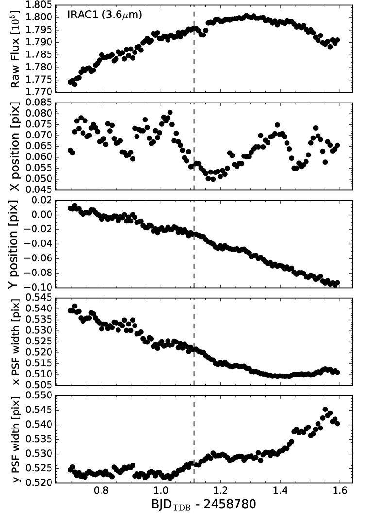
Figure 1: From top to bottom: Spitzer/IRAC1 (3.6 µm) photometry, stellar $x$ and $y$ positions relative to the (15, 15) pixel center, and PSF $x$ and $y$ widths, for our observations of LTT 9779. The vertical dashed line indicates the break between the two AORs.

For the Spitzer data, we first used POET to calculate aperture photometry for both IRAC channels with a range of aperture sizes, from 2.0 to 6.0 IRAC pixels and with inner and outer sky annulus radii of 7 and 15 pixels. Interpolated partial-pixel aperture photometry (with an oversampling factor of five) accounted for fractional pixels in the photometric calculations. To precisely track the location of the star we fit a Gaussian profile to the stellar profile in each frame, using a constant term to model each frame’s background flux. The raw flux, position, and PSF width are plotted in Figs. 1 and 2 for the 3.6 µm and 4.5 µm data, respectively.

POET models and removes IRAC’s well-known systematic correlation between a target’s measured flux and the position of the source within a pixel. Without properly accounting for this intra-pixel sensitivity effect, weak exoplanetary signals are (at best) difficult to accurately extract. POET accounts for this systematic effect using its bilinearly-interpolated sub-pixel sensitivity (BLISS) mode (Stevenson et al., 2012b). In BLISS mapping the main model hyperparameters are the choice of grid size for the sub-pixel sensitivity map, the astrophysical light curve model (e.g. phase curve, eclipses, transits), and any additional light-curve models to account for additional systematics (e.g. exponential ramp, correlation with PSF width, or other long-term trends), as well as the choice of photometric aperture size.

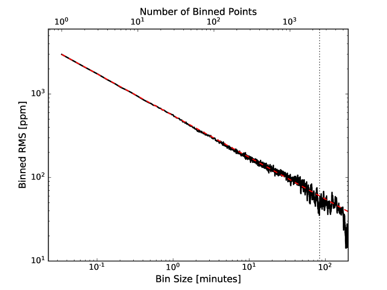
Figure 4: The dispersion of the binned residuals (solid line) to the 4.5 µm light curve (Fig. 3) shows no significant evidence for correlated noise. The dashed line shows the expectation for wholly uncorrelated errors, which scale as $N^{-1/2}$, and the vertical dotted line indicates the transit duration.

We followed past POET analyses of IRAC data by choosing the hyperparameters that minimize the standard deviation of the normalized residuals (SDNR) — essentially minimizing the scatter on the residuals to the full light-curve fit. However, to avoid overfitting we also followed POET’s recommendation to select the set of hyperparameters that minimizes SDNR but for which a nearest-neighbor interpolation does not outperform the BLISS interpolation. After testing a range of models, aperture sizes, and grid sizes (from 0.003 to 0.03 pixels), our final analysis identified the optimal set of parameters for the 4.5 µm channel as a 5-pixel photometric aperture, a 0.017 pixel grid scale, an astrophysical model including a transit, secondary eclipse, and sinusoidal phase curve, and a systematic model consisting of a quadratic correlation with PSF width. As described below, this model does a good job at accounting for the instrumental and astrophysical signals in the IRAC2 photometry; we achieve consistent final results with analyses using a four- or six-pixel apertures.. In Fig. 3 we show the calibrated IRAC2 photometry and best-fit light curve model. Fig. 4 shows that the residuals to our fit bin down approximately as white noise. Based on the WISE infrared flux of the star (Cutri & et al., 2014) and the IRAC system throughput (Spitzer Science Center, 2012), we calculate that our 4.5 µm photometry reaches 1.3$\times$ the expected photon noise limit.

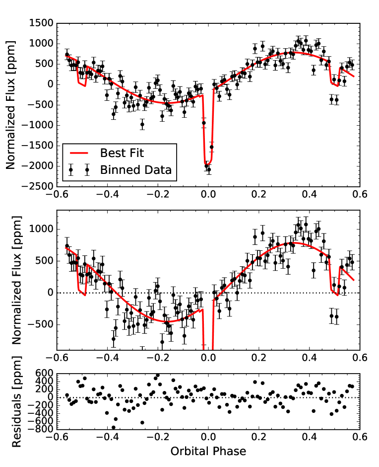
Figure 5: Spitzer/IRAC1 (3.6 µm) observations. From top to bottom: the full set of observations, the full data set again (but stretched to highlight the phase variations), and the residuals to the fit. The binned photometry is indicated by the black points, and the red line is the best-fit model. The best-fit model is nonphysical, requiring negative night-side flux. This model reaches only 2.3$\times$ the photon-noise limit (worse when restricted to physically plausible models) and the residuals exhibit considerable correlated noise (Fig. 6).

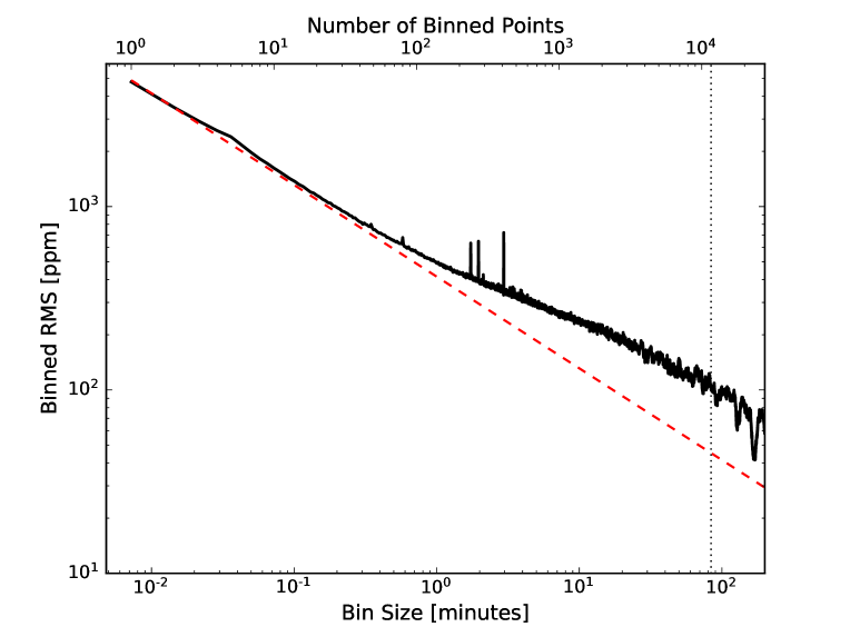
Figure 6: The dispersion of the binned residuals (solid line) to the 3.6 µm light curve (Fig. 5) shows significant evidence for correlated noise. The dashed line shows the expectation for wholly uncorrelated errors, which scale as $N^{-1/2}$, and the vertical dotted line indicates the transit duration.

However, for the 3.6 µm IRAC1 photometry our models that explain this channel’s instrumental and astrophysical variations imply a thermal phase curve with an implausibly large amplitude. These optimal models include a 2–3 pixel aperture, a BLISS grid size of 0.005 pixels, a linear ramp at the start of the first AOR, a correlation with PRF parameters, and a transit, secondary eclipse, and sinusoidal phase curve. In Fig. 5 we show the calibrated IRAC1 photometry and best-fit light curve model. Even after calibration the light curve shows high scatter, little or no sign of a secondary eclipses at the start of the observation (Eclipse 5 in the analysis of Dragomir et al., 2020), and the best-fit phase curve model would nominally hint at negative planetary flux between the transit and first eclipse. Fig. 6 shows that even when allowing nonphysical phase curve models, the residuals to our light curve fits bin down substantially slower than would be expected in the presence of white noise alone, further indicating the presence of systematic correlated noise not captured by the POET analysis. We calculate that our systematics-corrected 3.6 µm photometry still reaches only 2.3$\times$ the expected photon noise limit on short timescales, and substantially worse on longer timescales. Although the IRAC1 transit is recovered at high confidence, due to this data set’s intractable problems and high noise levels we do not further consider the 3.6 µm eclipses (which is discussed in more detail by Dragomir et al., 2020) or phase curve.

3.2 Spitzer eclipse, transit, and phase curve modeling

Although the main goal of this analysis is LTT 9779b’s phase curve (which we detect at 4.5 µm), we also observed two transits (one in each IRAC band). The eclipse analysis is described in more detail by Dragomir et al. (2020), who analyzed our eclipse observations together with four additional eclipses in each IRAC channel. Their measurement of the eclipse depth is necessarily more precise than ours would be, due to the larger number of eclipses analyzed. In our analysis we therefore hold the eclipse depth fixed at their derived value, 375 ppm (their analysis shows that the two eclipses shown in Fig. 3 have a depth consistent at 1.1$\sigma$ with the overall depth measured from all six eclipses). For other physical parameters (except where noted below), we use the system parameters of Jenkins et al. (2020).

Based on the stellar parameters from Jenkins et al. (2020), we used the 3.6 µm and 4.5 µm quadratic limb-darkening coefficients from Claret et al. (2013). The average limb-darkening coefficients corresponding to $T_{\mathrm{eff}}=5500$ K and $\log g=4.5$ are $u_{1}=0.106$ and $u_{2}=0.121$ (at 3.6 µm) and $u_{1}=-0.02$ and $u_{2}=0.33$ (at 4.5 µm). As noted previously, our IRAC2 primary transit occurs during a break in our Spitzer observations. This break makes the transit somewhat more challenging to model, so we elect to keep $u_{2}$ fixed at the tabulated value and allow $u_{1}$ to float within the range of values calculated by (Claret et al., 2013), i.e. in the range from $-0.13$ to $+0.09$.

For our phase curve modeling, we use a simple sinusoidal model with functional form

$$f(\phi)=1-A\cos(\phi-\Delta\phi)$$ (1)

where $\phi$ is the orbital phase (zero at transit, $\sim$0.5 at secondary eclipse), $A$ is the normalized (fractional) semi-amplitude, and $\Delta\phi$ is the phase offset (i.e., the planetary longitude corresponding to maximum flux). Since our final S/N on LTT 9779b’s IRAC2 phase curve is relatively low, more complicated models (e.g. including higher-order harmonics) were not justified by the data.

3.3 TESS Phase Curve Analysis

We also modeled the PDC (Pre-Search Data Conditioning) light curve of LTT 9779b (Smith et al., 2012; Stumpe et al., 2012, 2014) using the methodology presented by Daylan et al. (2019) to infer the planet’s phase modulation components at optical wavelengths.

We performed a global fit of the full PDC light curve using allesfitter (Günther & Daylan, 2019, 2020), an inference framework for joint modeling of light curve and radial velocity data. We modeled the light curve as the sum of the stellar baseline emission occulted by the planet during the primary transit, the planetary baseline emission occulted by the star during the secondary eclipse, the planetary modulation in the form of a cosine at the orbital period that peaks at superior conjunction, the ellipsoidal variation in the form of a cosine at half the orbital period that peaks at quadrature phases, and an additive constant offset to absorb any normalization bias. Although the planetary modulation can be subject to a phase shift, we nevertheless assumed a phase shift of zero (the value expected for reflected light and for thermal emission from such a hot planet). This is because the resulting planetary modulation amplitude was small, leaving the optical phase shift unconstrained. We also assumed a circular orbit. We modeled the data (which could consist of thermal emission, reflected starlight, or both) as a linear combination of the following components:

• planetary day side: $\frac{A_{d}}{2}(1-\cos 2\pi\phi)$ outside the secondary eclipse and 0 otherwise,

• planetary night side:, $\frac{A_{n}}{2}(1+\cos 2\pi\phi)$ outside the secondary eclipse,

• ellipsoidal variation, $A_{e}\sin 4\pi\phi$, i.e., a sinusoid at twice the orbital period that peaks at quadrature (0.25 and 0.75) phases,

• an additive constant offset to absorb any normalization bias.

$A_{d}$, $A_{n}$ and $A_{e}$ parameterize the amplitudes of these components.

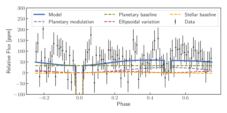
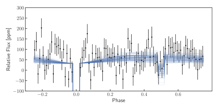
Figure 7: TESS optical-wavelength photometry of LTT 9779, shown by the black points and error bars. Top: The best-fit total model (blue) along with individual components. Bottom: Posterior distribution from our modeling analysis, showing a likely detection of the planet’s secondary eclipse but no clear detection of the planet’s phase variation.

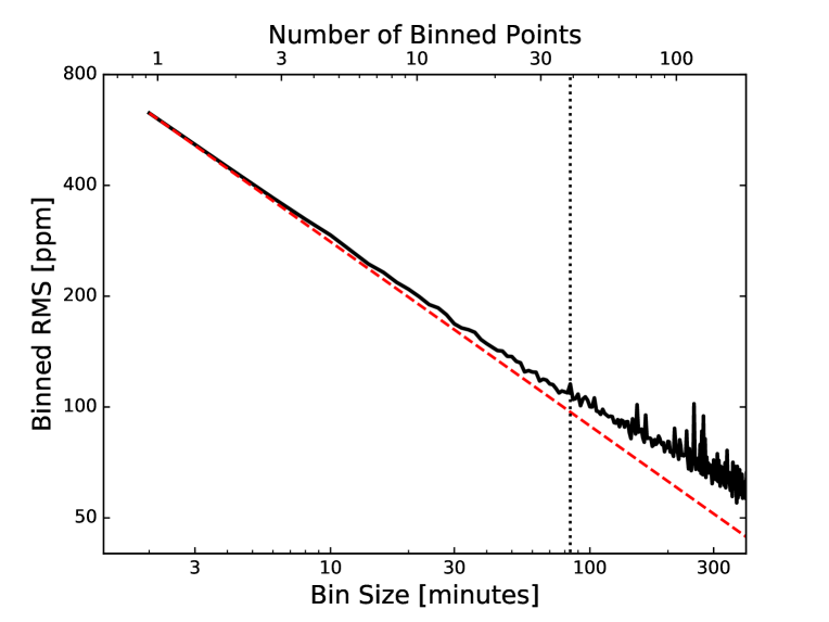
Figure 8: Same as Figs. 4 and 6, but for the TESS data shown in Fig. 7.

We sampled from the posterior distribution of the global model parameters using uniform priors. The posterior median phase curve components are shown in Fig. 7, where the black points denote the light curve phase-folded at the posterior median period and binned. The blue line shows the posterior median model fitted to the data. The colored dashed lines show the individual components of the posterior median model. The stellar baseline, planetary baseline, planetary modulation, and the ellipsoidal variation are shown in Figure 1 with orange, olive, magenta, and red colors, respectively. We obtain a secondary eclipse depth of $59^{+24}_{-21}$ ppm (Dragomir et al., 2020), a phase curve amplitude of $25^{+14}_{-13}$ ppm, and a night-side emission of $33^{+24}_{-20}$ ppm. The photometric precision we achieve is in line with expectations from the demonstrated performance of TESS: The star is TESS mag$=9$, so the expected photometric precision is roughly 100 ppm hr^-1/2 (Ricker et al., 2014). The phase curve plotted in Fig. 7 has been averaged down into 100 bins, each containing roughly 150 2-minute cadence measurements – i.e., 5 hr. So the expected 1$\sigma$ precision is $100/\sqrt{(}5)\approx 45$ ppm, consistent with our achieved precision. Fig. 8 shows how the residuals to our TESS analysis bin down over time, which suggests residual correlated noise of no more than 15% on the timescale of LTT 9779b’s transit duration.

4 Measurement and Interpretation

4.1 Spitzer Transits and an Updated Ephemeris

Our IRAC transits are mainly useful for refining the planet’s orbital ephemeris and reducing the uncertainty on its orbital period from that reported in the initial TESS analysis of Jenkins et al. (2020) and the updated analysis of Dragomir et al. (2020). Our 3.6 µm and 4.5 µm transit analyses yield mid-center times of $T_{0}=2458781.13997\pm 0.00032$ and $2458783.51684\pm 0.00053$, respectively (BJD_TDB). The IRAC1 and IRAC2 transits occurred 539 and 542 orbits, respectively, after the discovery epoch (Jenkins et al., 2020), which reported $T_{0}=2458354.21430\pm 0.00025$ and $P=0.7920520\pm 0.0000093$. With our new Spitzer transit times, a weighted least-squares fit gives an updated mid-transit time of $2458783.51636\pm 0.00027$ (BJD_TDB) and a refined period of $0.79207022\pm 0.00000069$ d, a measurement 13.6$\times$ more precise than the discovery period.

Our 3.6 µm and 4.5 µm transit depths are $R_{p}/R_{*}=0.0431\pm 0.0011$ and $0.0452\pm 0.0017$, respectively, consistent with the TESS transit depth (Jenkins et al., 2020). Neither the infrared nor the optical transit measurements are sufficiently precise to usefully constrain LTT 9779b’s atmosphere in transmission, because the planet’s expected scale height is relatively small (Jenkins et al., 2020).

Table 2: Properties of LTT 9779b

Parameter	Units	Value	1$\sigma$ Uncertainty	Notes
Fit Parameters:
$R_{p}/R_{*}$	—	0.0431	$\pm$0.0011	(3.6 µm; this work)
$R_{p}/R_{*}$	—	0.0452	$\pm$0.0017	(4.5 µm; this work)
$T_{0}$	BJDTDB	2458781.13997	$\pm$0.00032	(3.6 µm; this work)
$T_{0}$	BJDTDB	2458783.51684	$\pm$0.00053	(4.5 µm; this work)
$A$	ppm	358	$\pm$106	(4.5 µm; this work)
$\Delta\phi$	deg	$-10$	$\pm$$21$	(4.5 µm; this work)
Derived Parameters:
$T_{0}$	BJDTDB	2458783.51636	$\pm$0.00027	This work
$P$	d	0.79207022	$\pm$0.00000069	This work
$T_{\mathrm{day}}$	K	1800	$\pm$120	(4.5 µm, from Dragomir et al., 2020)
$T_{\mathrm{night}}$	K	700	$\pm$430	(4.5 µm; this work)
$\Delta T$	K	1110	$\pm$460	(4.5 µm; this work)

4.2 Phase curves

Our phase curve model (Eq. 1) can be used to determine the hemisphere-averaged flux and brightness temperature from the planet’s day and night sides. To effect this conversion, we use the BT-Settl library of synthetic stellar spectra (Allard, 2014) to properly model the non-blackbody stellar flux. We perform this calculation in a Monte Carlo framework in order to properly account for the uncertainties in both the secondary eclipse and phase curve amplitude. As expected, we also find that the large uncertainties on the phase curve parameters dominate the much smaller uncertainties in the stellar parameters.

We calculate 4.5 µm day and night-side temperatures of $T_{\mathrm{day}}=1800\pm 120$ and $T_{\mathrm{night}}=700\pm 430$, with upper limits on the night-side brightness temperature of $<1350$ K and $<1650$ K at 95.4% and 99.73% confidence (2$\sigma$ and 3$\sigma$), respectively. Note that our measurement of the day-side brightness temperature is somewhat more precise than that derived from the secondary eclipse analysis of (Dragomir et al., 2020), since our analysis also includes the full phase curve.

Combining the posterior distributions of the day- and night-side temperatures, we find a day-night temperature contrast of $\Delta T=1110\pm 460$ K. The distribution of $\Delta T$ is symmetric but non-Gaussian, with 95.4% and 99.73% (2$\sigma$ and 3$\sigma$) confidence intervals of $\pm 720$ K and $\pm 1030$ K, respectively. We also measure the planet’s phase offset (the longitude of maximum flux) to be $-10^{\rm o}\pm 21^{\rm o}$ east of the substellar point. Our full set of phase curve measurements from our Spitzer analysis are listed in Table 2.

In our TESS light curve analysis, we sampled from the posterior distribution of $A_{d}$, $A_{n}$ and $A_{e}$ (see Sec. 3.3) using uniform priors. The posterior median of these components are plotted against the TESS photometry in Fig. 7, along with the posterior median of the total model. As described by Dragomir et al. (2020), we find a TESS secondary eclipse depth of $55^{+24}_{-21}$ ppm (a roughly 3-$\sigma$ detection). However, the planet’s phase variation is not detected at high significance: we find a phase amplitude in the TESS bandpass of just $29\pm 17$ ppm. Further TESS observations of the system, anticipated in the TESS extended mission, would naturally improve the precision of these measurements.

4.3 General Circulation Models

Table 3: Phase Curve Properties

Bandpass	Source	Amplitude	Offset	$F_{P}/F_{*}$ [ppm] at:
		[ppm]	[deg]	$\phi=0$	$\phi=0.5$
TESS	data	$29\pm 17$	—	$33^{+24}_{-20}$	$59_{-21}^{+24}$
	Solar abundances	1.0	77	2.5	2.6
	$30\times$ Solar	7.8	41	4.7	10.7
Spitzer 4.5µm	data	$358\pm 106$	$-10\pm 21$	$17\pm 123$	$375\pm 62$
	Solar abundances	113	60	241	291
	$30\times$ Solar	261	23	272	511

To better interpret our observations of LTT 9779b, we calculated 3D general circulation models (GCMs) of this planet utilizing the SPARC/MITgcm (e.g., Showman et al., 2009). To reflect the range of possible observed atmospheric compositions we used two different model configurations, with atmospheric elemental abundances at the Solar level and 30$\times$ the solar level. Note that our simulations do not include the effect of atmospheric condensates, which some studies suggest could be important for planets even at these high temperatures (e.g., Parmentier et al., 2016). In particular, atmospheric aerosols would likely increase the geometric albedo in the TESS bandpass and so bring our GCM predictions into better agreement with the data at these shorter wavelengths.

Fig. 9 compares the 4.5$\mu$m and TESS phase curves predicted by our GCMs with our observations, and some relevant values for comparison are also enumerated in Table 3. At optical wavelengths, our GCMs predict lower flux than we observe with TESS at all orbital phases. At 4.5 µm, when compared to the observations the 30$\times$ Solar GCM predicts a hotter day side and smaller phase offset, while the Solar-abundance GCM predicts a somewhat cooler day side, smaller day-night temperature contrast, and larger phase offset. The trend seen in Fig. 9 of a phase curve amplitude that increases with atmospheric metallicity mirrors that seen in similar simulations for the similarly-sized, but much cooler, warm Neptune GJ 436b (Lewis et al., 2010). Nonetheless, neither of our GCMs provides an especially good match to our observations, which exhibit a much colder night side and smaller (consistent with zero) phase offset. Indeed, if anything the phase curve from the Solar-abundance GCM is a better match to our observations than is the 30$\times$ Solar model. And although our constraint on the phase offset is fairly loose, our measured day-side flux and phase curve amplitude both disagree with those predicted by the GCMs.

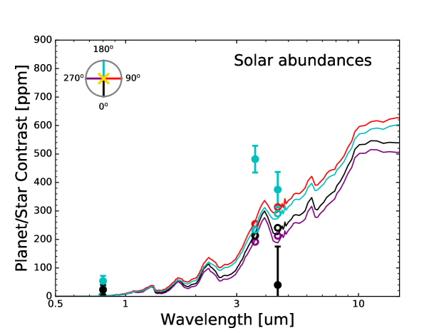
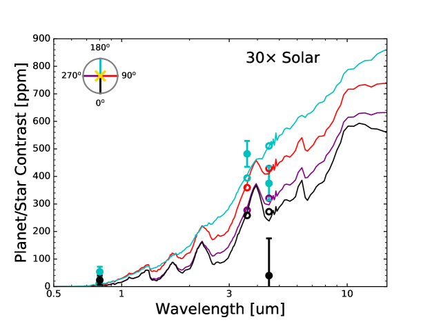
Figure 10: Planet/star contrast from our GCM simulations of LTT 9779b, assuming Solar abundances (left) and 30$\times$ Solar abundances (right), at four orbital phases. Black, night-side, as seen during transit (the planet’s night side); red, 90^o after transit; light blue, as seen during secondary eclipse (day side); and purple, 90^o after secondary eclipse. The solid points with error bars show the TESS and Spitzer measurements of the day- and night-side fluxes; the open circles indicate the band-averaged model points. The key in the top left corner is color-coded with the spectra to illustrate the sequence.

In Fig. 10, we also compare our measurements of the planet’s day- and night-side emission to the phase-resolved emergent spectra predicted by the GCMs. These reinforce the impressions conveyed by the comparison in Fig. 9 and Table 3: at 4.5 µm the Solar-abundance GCM over-predicts the night-side flux but under-predicts the day-side flux, while the 30$\times$-solar GCM over-predicts the planet’s flux at all phases; our (aerosol-free) GCMs underestimate the flux emitted in the TESS bandpass by 2.1$\sigma$ and 2.4$\sigma$ (for the Solar and 30$\times$ Solar abundance GCMs, respectively). On balance, the 30$\times$-solar GCM matches our observations somewhat better though (unlike Fig. 9) the comparison in Fig. 10 includes the 3.6 µm day-side (eclipse) measurement and so more strongly favors the 30$\times$-solar GCM ($\Delta\chi^{2}=15$), hinting at a super-Solar metallicity for LTT 9779b’s atmosphere. However, Fig. 10 also demonstrates that this model (unlike the Solar-abundance model) predicts a nearly isothermal day-side photosphere with only very weak spectral features, contrary to the strong absorption feature implied by the discrepant planetary brightness temperatures at 3.6 µm and 4.5 µm.

5 Discussion and Interpretation

5.1 Phase Curve interpretation

The large phase-curve amplitude and small phase offset in our 4.5 µm phase curve both suggest that LTT 9779b has a high-metallicity atmosphere. Higher-metallicity atmospheres have higher opacities, and Neptune-size planets may have atmospheric metallicities of 100$\times$ Solar or more (Fortney et al., 2013; Wakeford et al., 2017), much greater than expected for hot Jupiters. Therefore, the atmospheric layers probed by thermal emission measurements may tend to be at lower pressures for Neptunes than for Jovians, with consequently shorter radiative timescales. As a result, the phase curve offsets are expected to be smaller and the phase amplitudes larger than for the lower-metallicity hot Jupiters (Parmentier et al., 2018). Our phase offset measurement is not precise enough for a useful comparison, but the enhanced phase amplitude that we see suggests that LTT 9779b’s atmosphere may have an enhanced metallicity. The host star has a super-solar metallicity of [Fe/H]=+0.25 dex, but based on the GCM simulations shown in Fig. 9 the planet’s metallicity would be much more metal-rich, with [Fe/H]$\gtrsim 1.5$ dex.

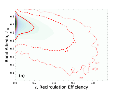
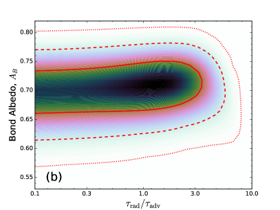
Figure 11: Probability distribution of atmospheric parameters derived from our 4.5 µm phase curve, with red lines indicating confidence intervals: 1$\sigma$ (solid), 2$\sigma$ (dashed), and 3$\sigma$ (dotted). Panel (a) shows Bond Albedo and energy recirculation efficiency, while panel (b) shows Bond Albedo and the timescale ratio $\tau_{\mathrm{rad}}/\tau_{\mathrm{adv}}$.

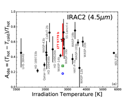
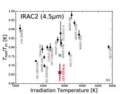
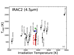
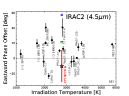
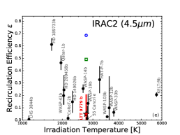
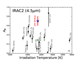
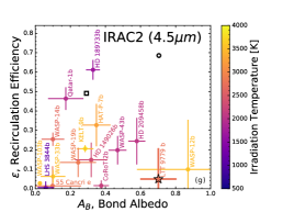
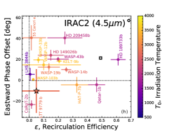
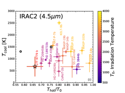
Figure 12: Derived parameters from all IRAC 4.5 µm phase curve measurements of planets on nearly-circular orbits. LTT 9779b is indicated by the red star, while our GCM predictions are indicated by the open blue circle (Solar metallicity) and green square (30$\times$ Solar).

We also used these brightness temperature with the radiative-balance model of Cowan & Agol (2011a) to estimate LTT 9779b’s Bond albedo $A_{B}$ and global heat recirculation efficiency $\epsilon$, as shown in Fig. 11a. In this framework, $\epsilon$ equals zero or unity, respectively, for zero circulation or full day-night recirculation. We find $\epsilon$=0.06$\pm$0.18 (2$\sigma$ upper limit of $<0.49$), indicating a very low level of heat redistribution consistent with the planet’s near-zero phase offset. For LTT 9779b’s Bond albedo we find a surprisingly high value of $A_{B}$=0.72$\pm$0.12 from our 4.5 µm data. Presumably this $A_{B}$ value is so high because CO and/or CO₂ absorb strongly in this planet’s atmosphere 4.5 µm (Dragomir et al., 2020), and so relatively less emission is seen in our IRAC2 observations. In this case, the high $A_{B}$ we derive would reflect the limits of single-band photometry for detailed energy balance calculations. Cowan & Agol (2011a) found that a single broadband infrared brightness temperature measurement translates into a roughly 8% systematic uncertainty in the effective temperature, and hence into a roughly 32% systematic uncertainty in bolometric flux and the Bond albedo. As a check on $A_{B}$, we repeated the calculation using the 3.6 µm eclipse measurement and assuming all 3.6 µm flux is emitted on the day side. In this case we calculate $A_{B}=0.27\pm 0.16$ (or $0.27^{+0.41}_{-0.26}$ at 99.73% confidence), which would not be remarkable in the context of the many hot Jupiters that have been studied in this way (see Fig. 12f).

On the other hand, LTT 9779b has $(R_{P}/a)^{2}=142$ ppm, which together with the TESS secondary eclipse indicates a geometric albedo in the TESS bandpass of roughly 0.4 if all the optical light were the result of scattering. A 2100 K blackbody would contribute only roughly 10 ppm of thermal emission at these wavelengths (see Fig. 9b), though such a planet’s spectrum is unlikely to closely resemble a blackbody. The optical data may therefore hint at a moderately high geometric albedo, which would differ qualitatively from the near-zero geometric albedo measured for some hot Jupiters (e.g. WASP-12b; Bell et al., 2017). Nonetheless, better flux measurements are needed to confirm this point.

Finally, we used a similar modeling approach to evaluate LTT 9779b’s 4.5 µm phase curve in terms of an alternative two-parameter model in which a planet’s global temperature distribution depends on $A_{B}$ and the ratio of radiative to advective timescales, $\tau_{\mathrm{rad}}/\tau_{\mathrm{adv}}$ (Cowan & Agol, 2011b, ; see the Appendix for some pedagogically useful analytic insights associated with this model). The posterior distribution of these parameters is shown in Fig. 11b, indicating $A_{B}$=0.71$\pm$0.04 (consistent with the measurement described immediately above) and a 2$\sigma$ upper limit of $\tau_{\mathrm{rad}}/\tau_{\mathrm{adv}}<3.8$ (consistent with expectations for such a hot planet).

To put LTT 9779b’s phase curve and derived parameters in the context of other 4.5 µm Spitzer phase curves, we followed the same procedures as described above to calculate $T_{\mathrm{day}}$, $T_{\mathrm{night}}$, $\Delta T$, $A_{B}$, and $\epsilon$ for all planets with published IRAC2/4.5 µm phase curves. These measurements are shown in Fig. 12, along with the predictions for LTT 9779b from our GCMs. We restrict this comparison to the sixteen planets with nearly-circular orbits (Knutson et al., 2012; Maxted et al., 2013; Zellem et al., 2014; Demory et al., 2016; Wong et al., 2015, 2016; Zhang et al., 2018; Kreidberg et al., 2018, 2019; Bell et al., 2019; Stevenson et al., 2017; Dang et al., 2018; Mansfield et al., 2020a; Keating et al., 2020).

Fig. 12 allows us to examine the sample of 4.5µm exoplanetary phase curves for possible trends between these planetary parameters. For example, Keating et al. (2019) and Beatty et al. (2019) claimed that the roughly uniform, $\sim$1100 K night-side temperatures of a sample of twelve hot Jupiters indicated the ubiquitous presence of night-side clouds. Our updated sample shows that this trend generally continues to hold, with the exceptions of hot Jupiters CoRoT-2b and KELT-9b (Dang et al., 2018; Mansfield et al., 2020a) and much smaller, presumed-rocky LHS 3844b (which has at most a tenuous atmosphere Kreidberg et al., 2019). In a similar vein, Zhang et al. (2018) used Spitzer phase curves of ten hot Jupiters to claim a coherent trend between $T_{\mathrm{irr}}$ and eastward phase offsets, which would indicate the increasing importance of magnetohydrodynamical effects at higher temperatures as well as high-altitude clouds. However, several recent measurements do not seem to support this trend, in particular the low phase offsets of Qatar-1b (consistent with zero shift at 2000 K Keating et al., 2020) and CoRoT-2b (a westward shift of $23\pm 4^{\mathrm{o}}$ at 2100 K Dang et al., 2018).

With two exceptions, the ensemble of 4.5 µm phase curve measurements depicted in Fig. 12 show that the parameters of LTT 9779b derived from its phase curve are generally similar to those of the population of hot Jupiters. The two exceptions, which stem from a single explanation, are that LTT 9779b exhibits an unusually low day-side temperature, and therefore has a high Bond albedo as derived from 4.5 µm observations (as discussed above), when compared to hot Jupiters with similar irradiation temperatures. These discrepancies are due to the 4.5 µm absorption feature inferred in LTT 9779b’s day-side spectrum (Dragomir et al., 2020). In contrast, most hot Jupiters at these temperatures exhibit more nearly blackbody-like day-side emission spectra due to shallower photospheric temperature gradients.

Observations inside molecular bands (e.g. the CO/CO₂ band at 4.5 $\mu$m) probe shallower atmospheric layers. This implies that our 3.6 $\mu$m phase curve should show a larger phase offset relative to the 4.5 $\mu$m phase curve, since it probes deeper into the atmosphere where energy re-radiation is less rapid and advective heat transport is more efficient. It is tempting to interpret the large phase offset apparently seen in the 3.6 µm phase curve (Fig. 5) as evidence of this phenomenon, but the nonphysical models required to explain this photometry (along with its high levels of correlated noise) caution against such an interpretation. Nevertheless, phase curves of this planet at additional wavelengths, probing a broader range of pressures, would provide a powerful diagnostic for measuring thermal structure and chemical abundances across the entire planet.

A particularly interesting comparison is between LTT 9779b and WASP-19b, an inflated hot Jupiter with multi-band eclipse and phase curve measurements (Wong et al., 2016, and references therein). The surface gravity and irradiation temperatures of these two planets are within 10% of each other, as shown in Table 4. Given two stars with such similar $T_{\mathrm{eff}}$ and $\log g$, one would expect any spectral differences to result solely from different metallicities; the same argument should presumably apply to planets as well. Yet WASP-19b has an essentially featureless day-side spectrum (unlike LTT 9779b) and the brightness temperature differences in the two Warm Spitzer bandpasses, $T_{\mathrm{day}}(3.6\,\micron)-T_{\mathrm{day}}(4.5\,\micron)$, is greater for LTT 9779b than for WASP-19b at 99.1% confidence. Table 4 also compares our hot Neptune to WASP-14b, another similarly-irradiated hot Jupiter but with 10$\times$ greater surface gravity. The case here is similar, with the two-color brightness temperature difference greater for LTT 9779b at 98.2% confidence. Although both additional data and further modeling are warranted, the different Spitzer emission spectra of LTT 9779b and WASP-14b & WASP–19b may be explained by the tendency of higher-metallicity atmospheres to show more strongly-decreasing thermal profiles at $T_{\mathrm{eq}}\lesssim 2300$ K (Mansfield et al., 2020b). Thus this comparison with hot Jupiters provides another tentative line of evidence that our target may have a significantly different (presumably higher) atmospheric metallicity than do hot Jupiters.

Table 4: Brightness Temperatures of Three Hot Exoplanets

Planet	WASP-14b	WASP-19b	LTT 9779b
Irradiation Temperature (K)	$2640\pm 43$	$2990\pm 50$	$2760\pm 33$
Planet Mass ($M_{\mathrm{Jup}}$)	$7.3\pm 0.5$	$1.114\pm 0.036$	$0.0922\pm 0.0025$
Planet Radius ($R_{\mathrm{Jup}}$)	$1.28\pm 0.08$	$1.395\pm 0.023$	$0.421\pm 0.021$
Surface Gravity ($\log_{10}$ [cgs])	$4.107\pm 0.043$	$3.152\pm 0.020$	$3.110\pm 0.044$
$T_{\mathrm{day}}$ (3.6 µm) (K)	$2341\pm 37$	$2361\pm 48$	$2305\pm 141$
$T_{\mathrm{day}}$ (4.5 µm) (K)	$2241\pm 45$	$2331\pm 67$	$1800\pm 120$
$T_{\mathrm{night}}$ (4.5 µm) (K)	$1301\pm 69$	$1130\pm 320$	$700\pm 430$
$T_{\mathrm{day}}(3.6\,\micron)-T_{\mathrm{day}}(4.5\,\micron)$ (K)	$100\pm 58$	$30\pm 82$	$510\pm 180$
$T_{\mathrm{day}}-T_{\mathrm{night}}$ (4.5 µm) (K)	$940\pm 78$	$1200\pm 330$	$1110\pm 460$

5.2 Conclusions and Future Prospects

One of the key goals of the ongoing TESS survey is to identify the best exoplanet targets for detailed atmospheric characterization (Ricker et al., 2014). TESS is already discovering such systems, opening wider the door to atmospheric studies of smaller planets. Among the most exciting TESS planets are those for which existing facilities can already answer new questions about the atmospheres of new classes of objects or of individual planets. LTT 9779 is such a system.

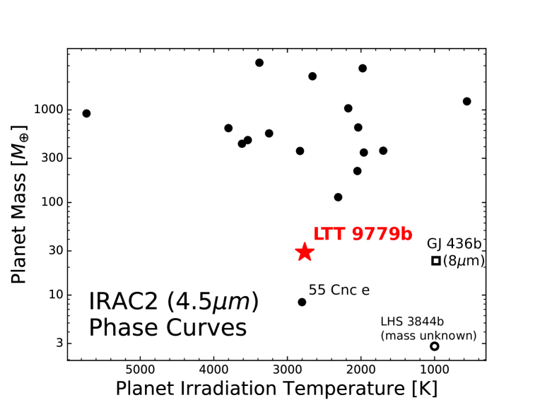
Figure 13: All planets with published Spitzer/IRAC2 (4.5 µm) phase curves. Only four planets with $M_{p}\lesssim 30M_{\oplus}$ have measured infrared phase curves: 55 Cnc e, LHS 3844b (whose mass is unknown), and GJ 436b (at 8 µm).

We have presented infrared and optical phase curve observations of this unusual hot Neptune, building on our analysis of its day-side emission spectrum through secondary eclipses in Dragomir et al. (2020). The planet’s phase curve is clearly seen in our Spitzer 4.5 µm photometry (Fig. 3); these data detect the signature of heat recirculation on this planet, with a $3\sigma$ confidence interval on the day-night temperature contrast of $1110\pm 1030$ K. Our observations plug a glaring gap, since Fig. 13 shows that no infrared phase curve data exist for any similar planet (i..e, within a factor of three of LTT 9779b’s mass and a factor of two of its temperature).

Overall, via several lines of evidence our measurements hint at an atmospheric metallicity enhanced above the Solar level. These arguments are mainly derived from the strong constraints placed on the planet’s global circulation patterns from the 4.5 µm phase curve. First, the eastward phase offset of $-10\pm 21^{\rm{o}}$ (to the west) is more consistent with that predicted by our general circulation models (GCMs) that are preferentially enhanced in heavy elements (see Fig. 9 and Table 3). Such a small phase offset also indicates a low heat recirculation efficiency and relatively small ratio of radiative to advective timescales, consistent with the values seen for hot Jupiters at comparable temperatures. In addition, LTT 9779b’s 4.5 µm phase curve amplitude of $358\pm 106$ ppm is also consistent with our enhanced-metallicity GCM predictions (see Fig. 9 and Table 3), though that model’s orbit-averaged infrared emission is elevated compared to our observations; future modeling at higher atmospheric metallicity and including the effects of aerosols may be needed to conclusively interpret our observations (cf.  Kataria et al., 2015; Parmentier et al., 2016; Keating et al., 2019). Including the 3.6 µm day-side observation in the GCM comparison (Fig. 10) also shows a better (though far from perfect) match between the observations and our higher-metallicty model.

Furthermore, the GCM predictions may also under-predict the planet’s optical-wavelength emission seen by TESS, though this result is more tentative (TESS is scheduled to observe LTT 9779b for another month-long sector in late 2020, which should tighten the measurements at optical wavelengths). The optical observations may hint at a nonzero geometric albedo, while the two-channel Spitzer measurements do not tightly constrain the planet’s Bond albedo.

Finally, further support for a high-metallicity atmosphere comes from our comparison of LTT 9779b’s thermal phase curve and day-side emission measurements with two similarly-irradiated hot Jupiters, WASP-14b and WASP-19b (see Table 4). In particular, although the surface gravity and irradiation temperature of WASP-19b differ from those of LTT 9779b by $<$10%, the two planets have qualitatively different emission spectra at $>99\%$ confidence. The hot Jupiters WASP-14b and WASP-19b both exhibit approximately featureless, pseudo-blackbody emission spectra devoid of spectral features, in contrast to the absorption inferred in our hot Neptune’s broadband emission spectrum (Dragomir et al., 2020); models also suggest that stronger absorption at this irradiation tempreature is consistent with a higher-metallicity atmosphere (Mansfield et al., 2020b).

The primary, two-year TESS mission is nearly complete. When done, 85% of the sky will have been surveyed for planets transiting nearby stars. To date, LTT 9779b remains one of the best targets of its type – i.e., among highly irradiated hot Neptunes that are highly favorable for thermal emission measurements – and so it is likely to remain one of the most easily-characterizable exoplanets in its class. Future phase curve and eclipse observations of LTT 9779b and other similar planets will provide the impetus for the next generation of global circulation modeling of Neptune-size planets, supporting similar observations of many such objects with JWST, ARIEL, and future observatories.

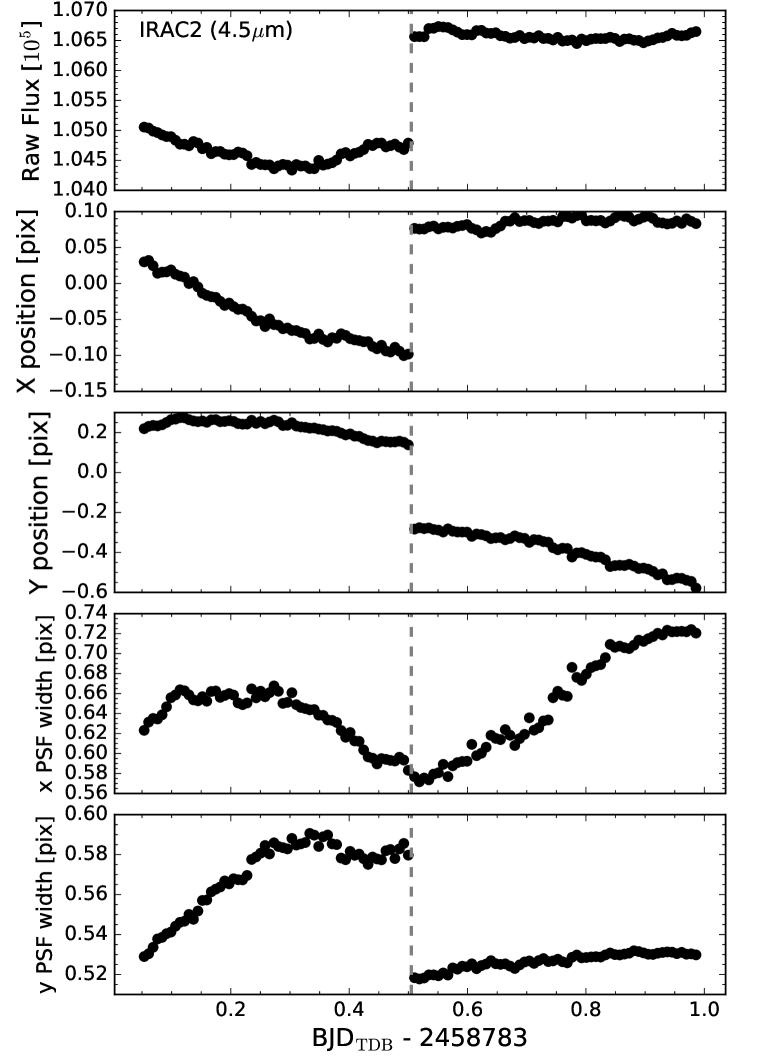
Figure 2: From top to bottom: Spitzer/IRAC2 (4.5 µm) photometry, stellar $x$ and $y$ positions relative to the (15, 15) pixel center, and PSF $x$ and $y$ widths, for our observations of LTT 9779. The vertical dashed line indicates the break between the two AORs.

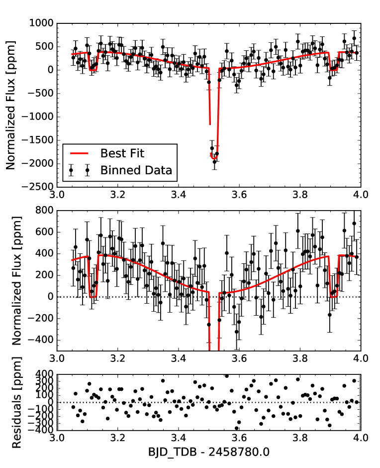
Figure 3: Spitzer/IRAC2 (4.5 µm) observations and phase curve. From top to bottom: the full set of observations, the full data set again (but stretched to highlight the phase variations), and the residuals to the fit. The binned photometry is indicated by the black points, and the red line is the best-fit model. These data reach 1.3$\times$ the photon-noise limit on short timescales and exhibit no sign of residual correlated noise (Fig. 4).

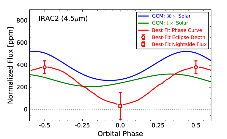
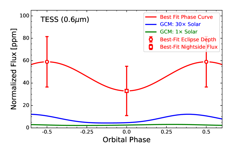
Figure 9: Best-fit model to our phase curve data (red curves) along with predicted phase curves from our general circulation models (blue and green curves). The gaps in the red curve indicate the times of secondary eclipse and primary transit; the error bars indicate the measured day-side flux (circles) and night-side flux (square). Neither GCM closely matches the observations, either at 4.5 µm (Spitzer, top) or at 0.6 µm (TESS, bottom).

Cowan & Agol (2011b) present a simple two-parameter model for atmospheric phase curves, in which a planet’s global temperature distribution is determined by the interplay between its Bond albedo, $A_{B}$, and the ratio of its radiative and advective timescales, $\varepsilon^{\prime}\equiv\tau_{\mathrm{rad}}/\tau_{\mathrm{adv}}$. We present here a further analytic approximation to this modeling framework which may be pedagogically useful.

This model assumes a coordinate system in which $\theta=0$ at the North pole and $\pi$ at the South pole, while $\phi=0$ at the substellar longitude, $-\pi/2$ at dawn, and $\pi/2$ at sunset. It defines planetary temperature $T$ in terms of $T^{\prime}=T/T_{\mathrm{irr}}$, where $T_{\mathrm{irr}}$ is a fiducial planetary temperature:

$$T_{\mathrm{irr}}\equiv T_{\mathrm{eff}}(1-A_{B})^{1/4}\sin^{1/4}\theta\left(\frac{R_{*}}{a}\right)^{1/2}.$$ (1)

Subject to energy balance, the temperature of gas parcels all around the planet are then the solutions to the differential equation

$$\frac{dT^{\prime}}{d\phi}=\frac{2\pi\tau_{\mathrm{adv}}}{\tau_{\mathrm{rad}}}\left(\max(\cos\phi,0)-{T^{\prime}}^{4}\right).$$ (2)

Cowan & Agol (2011b) provide an analytic solution to Eq. 2 for the planet’s night-side but numerical solutions are required for the day side. The analytic solution for the night-side temperature can be found by integrating from dusk (when the parcel stops absorbing energy, $\phi=\pi/2$) until some later phase $\phi$ (up until dawn, $\phi=3\pi/2$), and its solution is

$$T^{\prime}_{\mathrm{night}}(\phi)=\left(6\pi\frac{\tau_{\mathrm{adv}}}{\tau_{\mathrm{rad}}}\left[\phi-\frac{\pi}{2}\right]+(T^{\prime}_{\mathrm{dusk}})^{-3}\right)^{-1/3}.$$ (3)

On the planet’s day side, a second-order approximation can provide some additional insights hidden by the more exact (but numerically-derived) solution. By assuming that $T^{\prime}$ is a quadratic function of $\phi$ and expanding $\cos\phi\approx 1-\phi^{2}/2$, one obtains

$$T^{\prime}_{\mathrm{day}}\approx\left(1-\frac{\varepsilon^{\prime 2}}{64\pi^{2}}\right)+\frac{\varepsilon^{\prime}}{32\pi}\phi-\frac{1}{8}\phi^{2}.$$ (4)

This approximate analytic solution shows that the temperature of planetary gas reaches a maximum temperature at longitude

$$\phi_{\mathrm{max}}\approx\frac{1}{8\pi}\frac{\tau_{\mathrm{rad}}}{\tau_{\mathrm{adv}}}.$$ (5)

By setting $\phi=\phi_{\mathrm{max}}$ in Eq. 4, we obtain the temperature of the day-side hot spot:

$$T^{\prime}_{\mathrm{day,max}}=T^{\prime}_{\mathrm{day}}(\phi_{\mathrm{max}})\approx 1-\frac{7\varepsilon^{\prime 2}}{512\pi^{2}}.$$ (6)

As shown in Fig. 14, these approximate quadratic solutions are a decent match to the exact analytic solution for low $\tau_{\mathrm{rad}}/\tau_{\mathrm{adv}}$, though over-predicting somewhat the temperature at dawn and dusk. The approximation breaks down for $\tau_{\mathrm{rad}}/\tau_{\mathrm{adv}}\gtrsim 20$, when Eq. 6 becomes negative, but in this case the phase curve is nearly flat anyway.

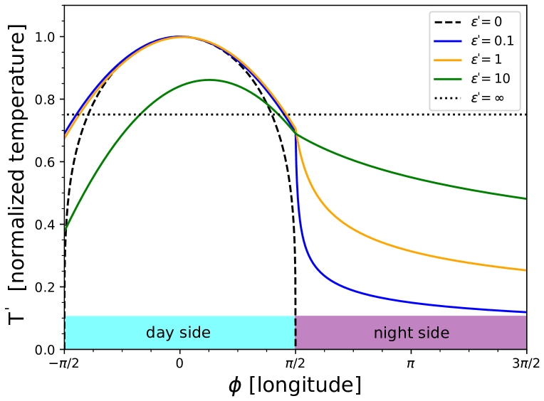
Figure 14: Planetary temperature vs. longitude for the simple energy transport model described in the appendix, for different values of $\varepsilon^{\prime}=\tau_{\mathrm{rad}}/\tau_{\mathrm{adv}}$. The substellar longitude is at $\phi=0$. The solid curves on the day side are the second-order analytic, approximate solutions of Eq. 4, while on the night side are plotted the exact solutions of Eq. 3. The broken black curves are the exact solutions for the limiting cases indicated, i.e. atmospheres dominated by radiation (dashed) and advection (dotted).

References

- Allard (2014) Allard, F. 2014, in IAU Symposium, Vol. 299, IAU Symposium, ed. M. Booth, B. C. Matthews, & J. R. Graham, 271–272
- Arcangeli et al. (2019) Arcangeli, J., Désert, J.-M., Parmentier, V., et al. 2019, A&A, 625, A136, doi: 10.1051/0004-6361/201834891
- Baxter et al. (2020) Baxter, C., Désert, J.-M., Parmentier, V., et al. 2020, A&A, 639, A36, doi: 10.1051/0004-6361/201937394
- Beatty et al. (2019) Beatty, T. G., Marley, M. S., Gaudi, B. S., et al. 2019, AJ, 158, 166, doi: 10.3847/1538-3881/ab33fc
- Bell et al. (2017) Bell, T. J., Nikolov, N., Cowan, N. B., et al. 2017, ApJ, 847, L2, doi: 10.3847/2041-8213/aa876c
- Bell et al. (2019) Bell, T. J., Zhang, M., Cubillos, P. E., et al. 2019, MNRAS, 489, 1995, doi: 10.1093/mnras/stz2018
- Bourrier et al. (2018a) Bourrier, V., Lovis, C., Beust, H., et al. 2018a, Nature, 553, 477, doi: 10.1038/nature24677
- Bourrier et al. (2018b) Bourrier, V., Dumusque, X., Dorn, C., et al. 2018b, A&A, 619, A1, doi: 10.1051/0004-6361/201833154
- Claret et al. (2013) Claret, A., Hauschildt, P. H., & Witte, S. 2013, A&A, 552, A16, doi: 10.1051/0004-6361/201220942
- Cowan & Agol (2011a) Cowan, N. B., & Agol, E. 2011a, ApJ, 729, 54, doi: 10.1088/0004-637X/729/1/54
- Cowan & Agol (2011b) —. 2011b, ApJ, 726, 82, doi: 10.1088/0004-637X/726/2/82
- Cowan et al. (2007) Cowan, N. B., Agol, E., & Charbonneau, D. 2007, MNRAS, 379, 641, doi: 10.1111/j.1365-2966.2007.11897.x
- Crossfield et al. (2018) Crossfield, I., Werner, M., Dragomir, D., et al. 2018, Spitzer Transits of New TESS Planets, Spitzer Proposal
- Crossfield et al. (2019) Crossfield, I., Benneke, B., Dragomir, D., et al. 2019, Multiwavelength Phase Curves of a TESS Hot Neptune, Spitzer Proposal
- Cubillos et al. (2013) Cubillos, P., Harrington, J., Madhusudhan, N., et al. 2013, ApJ, 768, 42, doi: 10.1088/0004-637X/768/1/42
- Cutri & et al. (2014) Cutri, R. M., & et al. 2014, VizieR Online Data Catalog, II/328
- Dang et al. (2018) Dang, L., Cowan, N. B., Schwartz, J. C., et al. 2018, Nature Astronomy, 2, 220, doi: 10.1038/s41550-017-0351-6
- Daylan et al. (2019) Daylan, T., Günther, M. N., Mikal-Evans, T., et al. 2019, arXiv e-prints, arXiv:1909.03000. https://arxiv.org/abs/1909.03000
- Demory et al. (2016) Demory, B.-O., Gillon, M., de Wit, J., et al. 2016, Nature, 532, 207, doi: 10.1038/nature17169
- Dragomir et al. (2020) Dragomir, D., Crossfield, I. J. M., Deming, D., et al. 2020, ApJ
- Fazio et al. (2004) Fazio, G. G., Hora, J. L., Allen, L. E., et al. 2004, ApJS, 154, 10, doi: 10.1086/422843
- Fortney et al. (2013) Fortney, J. J., Mordasini, C., Nettelmann, N., et al. 2013, ApJ, 775, 80, doi: 10.1088/0004-637X/775/1/80
- Guerrero et al. (submitted) Guerrero, N., Seager, S., Huang, X., Vanderburg, A., & Glidden, A. submitted, ArXiv e-prints. https://arxiv.org/abs/2999.99999
- Günther & Daylan (2019) Günther, M. N., & Daylan, T. 2019, allesfitter: Flexible star and exoplanet inference from photometry and radial velocity. http://ascl.net/1903.003
- Günther & Daylan (2020) —. 2020, arXiv e-prints, arXiv:2003.14371. https://arxiv.org/abs/2003.14371
- Heng & Showman (2015) Heng, K., & Showman, A. P. 2015, Annual Review of Earth and Planetary Sciences, 43, 509, doi: 10.1146/annurev-earth-060614-105146
- Howard et al. (2012) Howard, A. W., Marcy, G. W., Bryson, S. T., et al. 2012, ApJS, 201, 15, doi: 10.1088/0067-0049/201/2/15
- Jenkins (2002) Jenkins, J. M. 2002, ApJ, 575, 493, doi: 10.1086/341136
- Jenkins et al. (2016) Jenkins, J. M., Twicken, J. D., McCauliff, S., et al. 2016, in Society of Photo-Optical Instrumentation Engineers (SPIE) Conference Series, Vol. 9913, Software and Cyberinfrastructure for Astronomy IV, 99133E
- Jenkins et al. (2020) Jenkins, J. S., Díaz, M. R., Kurtovic, N. T., et al. 2020, Nature Astronomy, doi: 10.1038/s41550-020-1142-z
- Kataria et al. (2015) Kataria, T., Showman, A. P., Fortney, J. J., et al. 2015, ApJ, 801, 86, doi: 10.1088/0004-637X/801/2/86
- Keating et al. (2019) Keating, D., Cowan, N. B., & Dang, L. 2019, Nature Astronomy, 3, 1092, doi: 10.1038/s41550-019-0859-z
- Keating et al. (2020) Keating, D., Stevenson, K. B., Cowan, N. B., et al. 2020, AJ, 159, 225, doi: 10.3847/1538-3881/ab83f4
- Knutson et al. (2012) Knutson, H. A., Lewis, N., Fortney, J. J., et al. 2012, ApJ, 754, 22, doi: 10.1088/0004-637X/754/1/22
- Kreidberg et al. (2018) Kreidberg, L., Line, M. R., Parmentier, V., et al. 2018, AJ, 156, 17, doi: 10.3847/1538-3881/aac3df
- Kreidberg et al. (2019) Kreidberg, L., Koll, D. D. B., Morley, C., et al. 2019, Nature, 573, 87, doi: 10.1038/s41586-019-1497-4
- Lewis et al. (2010) Lewis, N. K., Showman, A. P., Fortney, J. J., et al. 2010, ApJ, 720, 344, doi: 10.1088/0004-637X/720/1/344
- Li et al. (2019) Li, J., Tenenbaum, P., Twicken, J. D., et al. 2019, PASP, 131, 024506, doi: 10.1088/1538-3873/aaf44d
- Line et al. (2011) Line, M. R., Vasisht, G., Chen, P., Angerhausen, D., & Yung, Y. L. 2011, ApJ, 738, 32, doi: 10.1088/0004-637X/738/1/32
- Mansfield et al. (2020a) Mansfield, M., Bean, J. L., Stevenson, K. B., et al. 2020a, ApJ, 888, L15, doi: 10.3847/2041-8213/ab5b09
- Mansfield et al. (2020b) Mansfield, M., Line, M., Bean, J., et al. 2020b, in Exoplanets 3 Conference
- Maxted et al. (2013) Maxted, P. F. L., Anderson, D. R., Doyle, A. P., et al. 2013, MNRAS, 428, 2645, doi: 10.1093/mnras/sts231
- May & Stevenson (2020) May, E. M., & Stevenson, K. B. 2020, AJ, 160, 140, doi: 10.3847/1538-3881/aba833
- Mazeh et al. (2016) Mazeh, T., Holczer, T., & Faigler, S. 2016, A&A, 589, A75, doi: 10.1051/0004-6361/201528065
- Menou (2012) Menou, K. 2012, ApJ, 744, L16, doi: 10.1088/2041-8205/744/1/L16
- Moses et al. (2013) Moses, J. I., Line, M. R., Visscher, C., et al. 2013, ApJ, 777, 34, doi: 10.1088/0004-637X/777/1/34
- Parmentier & Crossfield (2018) Parmentier, V., & Crossfield, I. J. M. 2018, Exoplanet Phase Curves: Observations and Theory (Springer International Publishing AG), 116
- Parmentier et al. (2016) Parmentier, V., Fortney, J. J., Showman, A. P., Morley, C. V., & Marley, M. S. 2016, ArXiv e-prints. https://arxiv.org/abs/1602.03088
- Parmentier et al. (2018) Parmentier, V., Line, M. R., Bean, J. L., et al. 2018, A&A, 617, A110, doi: 10.1051/0004-6361/201833059
- Rajpurohit et al. (2020) Rajpurohit, A. S., Allard, F., Homeier, D., Mousis, O., & Rajpurohit, S. 2020, arXiv e-prints, arXiv:2008.01288. https://arxiv.org/abs/2008.01288
- Ricker et al. (2014) Ricker, G. R., Winn, J. N., Vanderspek, R., et al. 2014, in Society of Photo-Optical Instrumentation Engineers (SPIE) Conference Series, Vol. 9143, Society of Photo-Optical Instrumentation Engineers (SPIE) Conference Series, 20
- Ricker et al. (2016) Ricker, G. R., Vanderspek, R., Winn, J., et al. 2016, in Society of Photo-Optical Instrumentation Engineers (SPIE) Conference Series, Vol. 9904, Proc. SPIE, 99042B
- Schwartz et al. (2017) Schwartz, J. C., Kashner, Z., Jovmir, D., & Cowan, N. B. 2017, ApJ, 850, 154, doi: 10.3847/1538-4357/aa9567
- Showman et al. (2009) Showman, A. P., Fortney, J. J., Lian, Y., et al. 2009, ApJ, 699, 564, doi: 10.1088/0004-637X/699/1/564
- Smith et al. (2012) Smith, J. C., Stumpe, M. C., Van Cleve, J. E., et al. 2012, PASP, 124, 1000, doi: 10.1086/667697
- Spitzer Science Center (2012) Spitzer Science Center. 2012, IRAC Instrument Handbook, v2.0.2, ed. IRAC Instrument and Instrument Support Teams
- Stevenson et al. (2012a) Stevenson, K. B., Harrington, J., Lust, N. B., et al. 2012a, ApJ, 755, 9, doi: 10.1088/0004-637X/755/1/9
- Stevenson et al. (2012b) Stevenson, K. B., Harrington, J., Fortney, J. J., et al. 2012b, ApJ, 754, 136, doi: 10.1088/0004-637X/754/2/136
- Stevenson et al. (2014) Stevenson, K. B., Désert, J.-M., Line, M. R., et al. 2014, Science, 346, 838, doi: 10.1126/science.1256758
- Stevenson et al. (2017) Stevenson, K. B., Line, M. R., Bean, J. L., et al. 2017, AJ, 153, 68, doi: 10.3847/1538-3881/153/2/68
- Stumpe et al. (2014) Stumpe, M. C., Smith, J. C., Catanzarite, J. H., et al. 2014, PASP, 126, 100, doi: 10.1086/674989
- Stumpe et al. (2012) Stumpe, M. C., Smith, J. C., Van Cleve, J. E., et al. 2012, PASP, 124, 985, doi: 10.1086/667698
- Twicken et al. (2018) Twicken, J. D., Catanzarite, J. H., Clarke, B. D., et al. 2018, PASP, 130, 064502, doi: 10.1088/1538-3873/aab694
- Vanderspek et al. (2019) Vanderspek, R., Huang, C. X., Vanderburg, A., et al. 2019, ApJ, 871, L24, doi: 10.3847/2041-8213/aafb7a
- Wakeford et al. (2017) Wakeford, H. R., Sing, D. K., Kataria, T., et al. 2017, Science, 356, 628, doi: 10.1126/science.aah4668
- Wong et al. (2015) Wong, I., Knutson, H. A., Lewis, N. K., et al. 2015, ApJ, 811, 122, doi: 10.1088/0004-637X/811/2/122
- Wong et al. (2016) Wong, I., Knutson, H. A., Kataria, T., et al. 2016, ApJ, 823, 122, doi: 10.3847/0004-637X/823/2/122
- Zellem et al. (2014) Zellem, R. T., Lewis, N. K., Knutson, H. A., et al. 2014, ApJ, 790, 53, doi: 10.1088/0004-637X/790/1/53
- Zhang et al. (2018) Zhang, M., Knutson, H. A., Kataria, T., et al. 2018, AJ, 155, 83, doi: 10.3847/1538-3881/aaa458