Spitzer Reveals Evidence of Molecular Absorption in the Atmosphere of the Hot Neptune LTT9779b

Abstract

Non-rocky sub-jovian exoplanets in high irradiation environments are rare. LTT9779b, also known as TESS Object of Interest (TOI) 193.01, is one of the few such planets discovered to date, and the first example of an ultra-hot Neptune. The planet’s bulk density indicates that it has a substantial atmosphere, so to investigate its atmospheric composition and shed further light on its origin, we obtained Spitzer IRAC secondary eclipse observations of LTT9779b at 3.6 and 4.5 $\mu$m. We combined the Spitzer observations with a measurement of the secondary eclipse in the TESS bandpass. The resulting secondary eclipse spectrum strongly prefers a model that includes CO absorption over a blackbody spectrum, incidentally making LTT9779b the first TESS exoplanet (and the first ultra-hot Neptune) with evidence of a spectral feature in its atmosphere. We did not find evidence of a thermal inversion, at odds with expectations based on the atmospheres of similarly-irradiated hot Jupiters. We also report a nominal dayside brightness temperature of 2305 $\pm$ 141 K (based on the 3.6 $\mu$m secondary eclipse measurement), and we constrained the planet’s orbital eccentricity to $e<0.01$ at the 99.7 % confidence level. Together with our analysis of LTT9779b’s thermal phase curves reported in a companion paper, our results set the stage for similar investigations of a larger sample of exoplanets discovered in the hot Neptune desert, investigations which are key to uncovering the origin of this population.

1 Introduction

To a large extent, the field of astronomy is the study of emergent radiation from distant objects in order to ascertain their compositions and physical properties. When it comes to extrasolar planets, although thousands of planets are known to transit their host stars we often obtain the greatest insights into the much smaller set of planets whose thermal emission properties have been precisely measured.

Although the most precise thermal emission measurements come from directly imaged planets, these weakly-irradiated, long-period objects are structurally different than, and so only imperfect analogues for, the atmospheres of highly-irradiated, short-period planets. Thermal emission via secondary eclipse observations has been measured in dozens of hot Jupiters with few-band Spitzer (Werner et al., 2004) photometry. Though the wavelength coverage of such data is necessarily sparse, several trends have emerged. For example, hot Jupiters with $T_{\mathrm{eq}}\gtrsim 2200$ K are consistent with zero Bond albedo and inefficient global heat redistribution, indicating bright, hot daysides and relatively cold, dark night sides (Garhart et al., 2020). Furthermore, hot Jupiters with $T_{\mathrm{eq}}\gtrsim 1900$ K have consistent dayside brightness temperatures in the 3.6µm and 4.5µm Spitzer IRAC bandpasses (Garhart et al., 2020; Baxter et al., 2020). In addition, the hottest planets, such as the so-called “ultra-hot Jupiters,” also show qualitatively different atmospheres in which opacity from H^-, hydrides, and other non-oxides begin to play a much larger role than in the (relatively) cooler population (Arcangeli et al., 2018; Lothringer et al., 2018; Mikal-Evans et al., 2019).

Despite being relatively easy to discover in early surveys, the intrinsic occurrence of hot Jupiters is much lower than that of smaller planets (Howard et al., 2010; Fulton & Petigura, 2018). An apparently similar shortage of smaller, hot planets, deemed the hot Neptune desert, has been recognized more recently (Szabó & Kiss, 2011; Mazeh et al., 2016). This desert may have formed through mass loss of sub-Jovian-sized planets, via mechanisms such as photoevaporation (Owen & Lai, 2018) or Roche Lobe Overflow (Valsecchi et al., 2015).

Table 1: Spitzer Observations of LTT9779

Channel	Integration time (s)	AOR Start [UT]	AOR End [UT]	AOR No.	Aperture radius	$\beta$	Notes
					(pixels)
3.6	0.4	02/26/19 23:30	02/27/19 02:42	68701696	3.0	1.21	Ch1 eclipse 1
3.6	0.4	03/02/19 03:42	03/02/19 06:54	68697600	3.0	1.36	Ch1 eclipse 2
3.6	0.4	03/07/19 16:31	03/07/19 19:42	68694528	3.0	1.13	Ch1 eclipse 3
3.6	0.4	03/12/19 10:44	03/12/19 13:56	68699648	3.0	1.34	Ch1 eclipse 4
4.5	2.0	03/19/19 13:43	03/19/19 16:53	68695808	4.0	1.15	Ch2 eclipse 1
4.5	2.0	03/21/19 03:46	03/21/19 06:56	68700928	4.0	1.18	Ch2 eclipse 2
4.5	2.0	03/26/19 16:36	03/26/19 19:46	68697088	4.0	1.22	Ch2 eclipse 3
4.5	2.0	04/01/19 05:56	04/01/19 09:06	68695552	4.0	1.20	Ch2 eclipse 4
3.6	0.4	10/24/19 03:38	10/24/19 14:31	70006528	3.0	1.19	Ch1 eclipse 5 & $\frac{1}{2}$ phase curve
3.6	0.4	10/24/19 14:35	10/25/19 02:09	70007040	3.0	1.22	Ch1, eclipse 6 & $\frac{1}{2}$ phase curve
4.5	2.0	10/26/19 13:03	10/26/19 23:55	70005504	4.0	1.15	Ch2, eclipse 5 & $\frac{1}{2}$ phase curve
4.5	2.0	10/27/19 12:00	10/27/19 11:35	70006016	4.0	1.26	Ch2, eclipse 6 & $\frac{1}{2}$ phase curve

Because of the hot Neptune desert, few sub-Jovian planets with hot-Jupiter levels of irradiation ($T_{\mathrm{eq}}\gtrsim 1000$ K) are suitable for thermal emission measurements, and so such studies have largely focused on two disjoint sets: large, highly-irradiated hot Jupiters and smaller, cooler warm Neptunes (e.g. Wallack et al., 2019).

A new target excellently suited to bridge the gap between these two populations via secondary eclipse measurements of atmospheric composition and structure is the new ultra-hot Neptune LTT9779b (Jenkins et al. 2020). The TESS mission revealed this 4.6$\pm 0.2$ $R_{\oplus}$, 29.3$\pm 0.8$ $M_{\oplus}$ exoplanet on a 0.8 d orbit around its G dwarf host star, giving it an equilibrium temperature of roughly 2000 K. The combination of intense irradiation and sub-Jovian size and mass (which imply a 9% atmosphere by mass; Jenkins et al. 2020) makes LTT9779b a rare inhabitant of the hot Neptune desert, while its bright host star ($K_{s}=8.0$ mag) makes it the highest-S/N target for secondary eclipse measurements among known sub-Jovian planets. Measurements of the atmospheric composition of this desert-dwelling planet could shed light on the process by which it came to be, and on how this region of parameter space is cleared.

2 Spitzer Observations

Observations of LTT9779 were obtained in both Warm Spitzer IRAC channels (Fazio et al., 2004). Assuming a circular orbit for LTT9779b, we determined the most likely secondary eclipse times. For each channel, we scheduled Spitzer Astronomical Observing Requests (AORs) to overlap with four separate eclipse times (GO: 14084; Crossfield et al., 2018). Two additional secondary eclipse time series (per channel) were obtained from AORs that covered a full phase curve of the planet in each channel (which included two consecutive secondary eclipses; DDT 14290, Crossfield et al., 2019). The dates of all the Spitzer observations are listed in Table 1. The eight GO 14084 science AORs are 3.2 hours long. Each of the two GO 14290 phase curve time series spanned 22.5 hours. Exposure times were 0.4 s and 2 s for channel 1 and 2 observations, respectively.

We obtained the observations in subarray mode to reduce the data volume generated and better resolve short-timescale pointing jitter. Each eclipse-only science AOR was preceded by a 30-minute Pointing Calibration and Reference Sensor (PCRS) peak-up observation (Ingalls et al., 2012). Since each of the two phase curve observations consisted of two consecutive science AORs, just one PCRS observation prior to the first AOR of each phase curve was sufficient. The PCRS peak-up AORs help minimize instrumental noise from intra-pixel sensitivity variations by eliminating the initial large drift that often occurs when the telescope slews to the target. The PCRS step also allows for the target to settle on the “sweet spot” of a well-characterized pixel (Ingalls et al., 2012). We do not use the 30-minute PCRS observations in our analysis. Table 1 lists the details of all 12 of our Spitzer eclipse observations of LTT9779b.

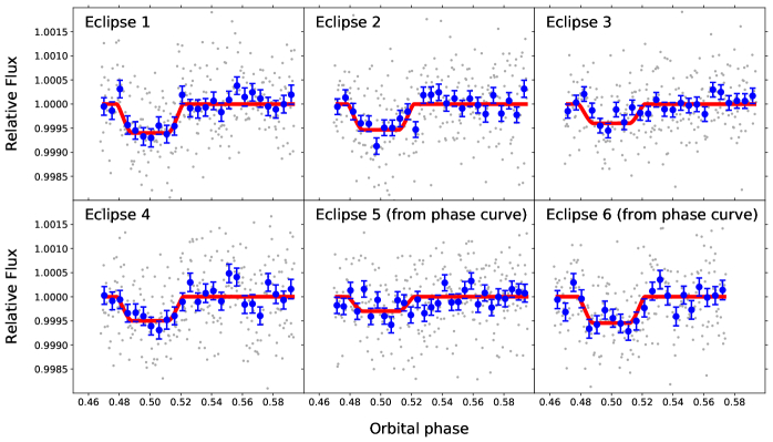
Figure 1: Individual Spitzer IRAC channel 1 (3.6µm) eclipses of LTT9779b. Gray and blue points correspond to the unbinned and 6-min. binned corrected light curves, respectively. The best-fit model for each individual eclipse fit is shown in red.

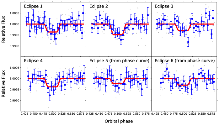
Figure 2: Individual Spitzer IRAC channel 2 (4.5µm) eclipses of LTT9779b. Gray and blue points correspond to the unbinned and 6-min. binned corrected light curves, respectively. The best-fit model for each individual eclipse fit is shown in red. Note that the vertical scale differs from Fig. 1.

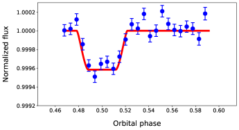
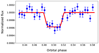
Figure 3: Phase-folded Spitzer IRAC channel 1 (left) and channel 2 (right) secondary eclipse corrected light curves of LTT9779b. Blue points correspond to 6-min. bins. The best-fit model is shown in red.

2.1 Photometric Extraction and Light Curve Analysis

We used the basic calibrated data (BCD) to extract light curves for a total of 12 eclipses, six in each channel. The BCD files are data cubes consisting of 64 images of 32 $\times$ 32 pixels. We follow a procedure similar to those described in previous works (e.g. Stevenson et al. 2012; Deming et al. 2015). For every image we subtract the sky background, we replace at each pixel position 4$\sigma$ outliers with the time median value for that pixel, and we use a 2D Gaussian fit to measure the centroid position of the stellar point spread function (PSF). Lastly, we sum the flux within eight circular apertures with a range of radii between 2 and 5 pixels.

For each 64-image data cube we reject 5$\sigma$ outliers from the cube median flux, and 10$\sigma$ outliers from the cube median x and y centroid position. We bin the remaining images in each data cube to obtain our raw light curve, and reject any points that are more than 4$\sigma$ from the median of the light curve flux.

We began the light curve analysis by trimming off the first 30 minutes of each one secondary eclipse light curve, which show a time-dependent ramp (Demory et al., 2011; Deming et al., 2011) that is not well fitted by the Pixel Level Decorrelation (PLD) method (Deming et al., 2015) that we used to correct the systematics present in the light curves.

We used PLD to remove the correlated noise in the flux time series caused by pointing jitter combined with intra-pixel sensitivity variations of Spitzer IRAC. We select an array consisting of the 9 pixels that contain most of the flux from the star, and model the instrument systematics with a linear combination of the fluxes in those pixels (to correct the correlated noise due to the pointing jitter) and either a first or second order polynomial in time (to correct the component of the correlated noise that is due to temporal effects in detector sensitivity; Demory et al. 2012):

Table 2: Spitzer Secondary Eclipse Depths and Times

Eclipse ID	Wavelength	Eclipse depth	Mid-eclipse time (BJD)
E1Ch1	3.6	600 $\pm$ 112	2458541.5374 $\pm$0.0011
E2Ch1	3.6	535 $\pm$ 128	2458544.7043${}^{+0.0020}_{-0.0016}$
E3Ch1	3.6	450 $\pm$ 111	2458550.2491${}^{+0.0023}_{-0.0026}$
E4Ch1	3.6	505 $\pm$ 125	2458555.0024 $\pm$ 0.0013
E5Ch1	3.6	320 $\pm$ 121	2458780.7396${}^{+0.0051}_{-0.0067}$
E6Ch1	3.6	546 $\pm$ 123	2458781.5334 $\pm$ 0.0013
Global Ch1	3.6	482 $\pm$ 47	2458541.53906$\bm{{}^{+0.00083}_{-0.00074}}$
E1Ch2	4.5	362 $\pm$ 131	2458562.1308${}^{+0.0016}_{-0.0020}$
E2Ch2	4.5	480 $\pm$ 137	2458563.7159 $\pm$ 0.0017
E3Ch2	4.5	301 $\pm$ 176	2458569.2599${}^{+0.0020}_{-0.0028}$
E4Ch2	4.5	348 $\pm$ 136	2458574.8022${}^{+0.0023}_{-0.0029}$
E5Ch2	4.5	236 $\pm$ 184	2458783.1160${}^{+0.0028}_{-0.0035}$
E6Ch2	4.5	282 $\pm$ 145	2458783.9049${}^{+0.0034}_{-0.0040}$
Global Ch2	4.5	372 $\pm$ 55	2458562.13302 $\pm$ 0.00092

$$\begin{split}S(t)=\sum c_{i}P_{i}(t)+ft(+gt^{2}),\end{split}$$ (1)

where $P_{i}(t)$ are the values of each of the 9 pixels as a function of time, $c_{i}$ are the coefficients associated with each $P_{i}(t)$ time series, $f$ (and $g$) are the linear (and quadratic) polynomial coefficients of the second order polynomial, and $t$ is the time. We compute the Bayesian Information Criterion (BIC Schwarz 1978) for all individual eclipse fits, using either a first-order polynomial (BIC_1st) or a second-order polynomial (BIC_2nd). If $\Delta$BIC$=$BIC${}_{2nd}-$BIC_1st is positive, we determine that the former represents the data well; if $\Delta$BIC is negative, the latter is needed to adequately model the temporal detector sensitivity effects. A second-order polynomial is strongly preferred for the channel 1 light curves ($-41<\Delta$ BIC $<-4$), while a first-order polynomial (i.e. linear function of time) is moderately preferred for the channel 2 light curves ($1<\Delta$ BIC $<4$). We model the light curves accordingly. While the planet’s phase curve is present and detectable in the light curves (see Crossfield et al., in review for an analysis of the thermal phase curves), we find that employing a second order polynomial is sufficient to flatten the out-of-eclipse portions of the light curves without the need for computationally intensive phase curve fits. In our systematics model, we omit the constant $h$ that Deming et al. (2015) include in their systematics model because the first term of equation 1 also serves to scale the out-of-transit level of the light curve, so this constant is not necessary (Benneke et al., 2017). We fit our data with the product of equation 1 and the eclipse model ($E(t)$):

$$\begin{split}F(t)=S(t)\cdot E(t),\end{split}$$ (2)

where $E(t)$ is analogous to the non-limb darkened transit model of Mandel & Agol (2002), except that the depth of the occultation represents the planet-to-star flux ratio (assuming the planet is a uniformly bright disk) rather than the planet-to-star area ratio. We fix the orbital period ($P$), scaled semi-major axis ($a/R_{S}$), orbital inclination ($i$) and planet-to-star radius ratio ($R_{P}/R_{S}$) to the values reported in Jenkins et al. (2020), which are constrained with much better precision by the 38 TESS transits they analyzed than we could achieve with the Spitzer eclipses. Specifically, we use $P=0.7920520\pm 0.0000093$, $a/R_{S}=3.877^{+0.090}_{-0.091}$, $i=76.39\pm 0.43$ and $R_{P}/R_{S}=0.0455^{+0.0022}_{-0.0017}$. Thus, we only fit for the mid-eclipse time and the eclipse depth $D$, as well as a scaling factor on the per-point photometric uncertainty $\beta$ (to ensure realistic uncertainties on the astrophysical parameters; e.g. Pont et al. 2006; Demory et al. 2016). We use the Python package scipy.optimize with the L-BFGS-B method (Byrd et al., 1995) to find a best fit solution which we use to initialize our MCMC algorithm, which uses the emcee code (Foreman-Mackey et al., 2013). We perform the fit on light curves extracted from apertures with radii between 2 and 5 pixels. For our final results, we used the aperture that minimizes the photometric uncertainties and the correlated noise component (i.e. the fitted scaling factor mentioned above), which are those with 3 and 4 pixel radii, for channels 1 and 2, respectively.

We fit each of the 12 eclipse light curves individually, and we also perform a global fit on the six light curves for each channel. Table 2 lists the best-fit values for the individual and global (in bold) eclipse depths and times from the MCMC runs. We also report the $\beta$ values in Table 1. Plots of the systematics-corrected light curves are shown in Figures 1 and 2. We show the combined light curves for channel 1 and 2 in Figure 3.

Additional independent analyses were performed by three of our team members (two using their own versions of PLD and one using BLISS, Stevenson et al. 2012), who found secondary eclipse values that agree with those shown in Table 2 to within 0.6$\sigma$ (for each Spitzer channel). In particular, all analyses found shallower eclipses in channel 2.

3 TESS Observations

The LTT9779 system was observed by the TESS spacecraft in Sector 2. To measure the TESS-band secondary eclipse depth and search for a possible visible-light phase curve signal from LTT9779b, we undertook two independent analyses of analyzed the Presearch Data Conditioning-Simple Aperture Photometry (PDC-SAP; Smith et al. 2012; Stumpe et al. 2014) light curve, which was processed through the Science Processing Operations Center (SPOC) pipeline (Jenkins et al., 2016) and has a 2-minute cadence. The PDC process is designed to correct the light curve for systematics while preserving astrophysical variability intrinsic to the target.

3.1 Light Curve Analysis

For the analysis we followed the methods described in detail in Shporer et al. (2019) and Wong et al. (2020). We first removed all flagged data points from the time series and applied a 16-point-wide moving median filter to trim $3\sigma$ outliers. Then, the light curve was broken up into segments that are separated by the scheduled momentum dumps, which occurred ten times during Sector 2. We ignored the two short $<$0.5-day segments that immediately preceded the data downlink interruptions, arriving at a total of 10 segments. Segments 3 and 9 were affected by significant flux ramps prior to the subsequent momentum dumps, so we trimmed the last 0.75 day worth of data from those two segments. The full light curve used in our analysis includes 16433 points, and contains 29 transits and 30 secondary eclipses.

The system’s normalized brightness variation was modeled as

$$F(t)=S(t)\cdot\frac{1+\bar{f}_{p}-A\cos(2\pi\phi)}{1+\bar{f}_{p}},$$ (3)

where $S(t)$ is a set of generalized polynomials in time used to model the long-term systematics trends (as defined in equation 5 of Shporer et al. 2019); $\phi$ is the orbital phase (with the zeropoint set at mid-transit); and the variables $\bar{f}_{p}$ and $A$ represent the average relative brightness of the planet across its orbit and the semi-amplitude of the phase curve variation, respectively. By definition, the secondary eclipse depth is $D=\bar{f}_{p}+A$. We assumed zero eccentricity to fix the mid-eclipse time to $\phi$ = 0.5.

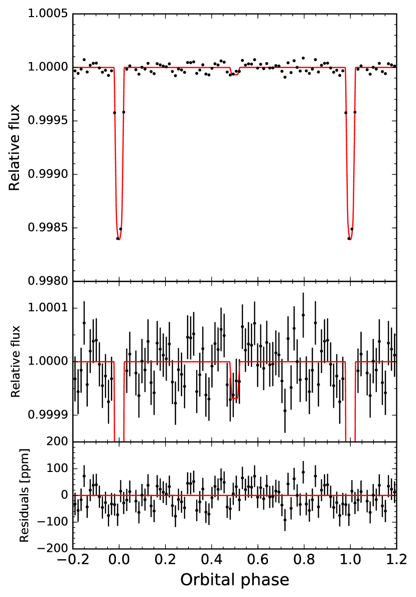
Figure 4: Top panel: TESS light curve of LTT9779 after correction of the long-term systematics trends, phase-folded on the period of LTT9779b and binned in 15 minute intervals (black points). The best-fit full phase curve model from our joint analysis is shown by the red curve. Upper middle panel: zoomed-in view of the secondary eclipse and out-of-eclipse light curve. Lower middle panel: Corresponding residuals from the best-fit model.

We modeled the transits and secondary eclipses using BATMAN (Kreidberg, 2015), and the phase curve using Equation (3). We allowed both the orbital ephemeris ($T_{0}$, $P$) and the transit shape parameters ($b$, $a/R_{*}$) to vary freely. The median and $1\sigma$ uncertainties on all parameters were computed using emcee (Foreman-Mackey et al., 2013). The values of Jenkins et al. (2020) were used as initial guesses for the transit parameters, while $\bar{f}_{p}$ and $A$ were initialized at 100 and 0 ppm, respectively. To ensure that the reduced chi-squared value is near unity and produce realistic uncertainties on the astrophysical parameters, we included a scaling factor on the per-point photometric uncertainty ($\beta$) as a free parameter.

No significant phase curve signal was detected, with the best-fit amplitude $A$ being consistent with zero to within $1\sigma$. Therefore, for our final results we opted to fix the phase curve amplitude to zero and the time of secondary eclipse to phase 0.5. We measured a marginal secondary eclipse depth of $D=69_{-26}^{+28}$ ppm. The systematics-corrected, phase-folded and binned light curve is shown in the two upper panels of Figure 4.

We also performed an independent analysis of the TESS light curve using allesfitter (Günther & Daylan, 2019) following a methodology similar to that presented in Daylan et al. (2019), and found an eclipse depth of $D=59_{-21}^{+24}$ ppm. This is in very good agreement with the value reported above, which we thus use for the remainder of the paper.

4 Atmosphere Modelling

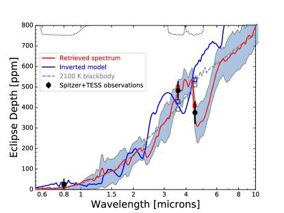
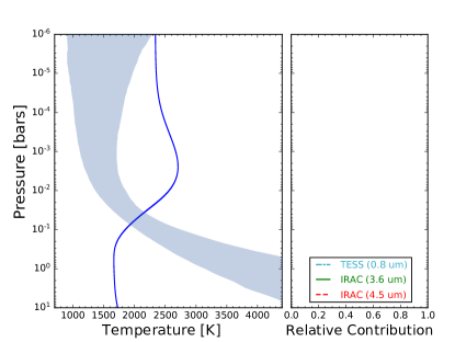
Figure 5: Left: Secondary eclipse measurements (black circles with error bars) with our weighted best-fitting model spectrum (red curve). The shaded region indicates the 68% confidence interval from our retrieval analysis, and the dotted lines indicate the TESS and IRAC filter responses. The dashed line shows the planet/star flux ratios for a planet with blackbody emission at a temperatures of 2100 K. An inverted model is shown for reference (in blue). Middle: Retrieved thermal profile (solid line) with 68% confidence interval (shaded region). The temperature decreases across the entire range of probed pressures. An inverted thermal profile is also shown (in blue). Right: Contribution functions for the TESS and IRAC bandpasses from the best-fit model spectrum.

4.1 Dayside brightness temperatures

Before analyzing the thermal emission spectrum of LTT9779b, we must take into account the fact that the planet’s albedo likely contributes non-negligibly to the depth of the TESS secondary eclipse. We thus determine an upper limit on the thermal emission that can originate from the planet in the TESS bandpass. Since the 4.5 $\mu$m eclipse depth suggests molecular absorption at that wavelength (see below and section 4.2), we take the brightness temperature at 3.6 $\mu$m to be a more accurate estimate of the planet’s dayside temperature. Using a stellar spectrum obtained with the BT-SETTL version of the PHOENIX atmospheric models (Allard et al., 2013), we find a 3.6 $\mu$m brightness temperature of 2305 $\pm$ 141 K. For reference, the planet’s equilibrium temperature is 1978 $\pm$ 19 K (Jenkins et al. 2020). Assuming a Bond albedo of 0 and that the planet re-emits all the flux it absorbs at the in the IRAC channel 1 bandpass, we find that the contribution from thermal emission to the TESS secondary eclipse is 27 ppm. We use this value for the analyses presented in the remainder of this Letter (but we note that even assuming a 0 ppm thermal emission contribution to the TESS secondary eclipse depth gives nearly identical results for the retrieval analysis we present in the next subsection).

We also fit a blackbody to the planet’s three-point spectrum. We find the brightness temperature corresponding to the best-fit model to be 2100 $\pm$ 188 K (see dashed gray line in Figure 5). However, the three eclipse depths are not well fitted by a blackbody emission spectrum. We interpret this as evidence of molecular absorption originating from the planet’s atmosphere at 4.5 $\mu$m, which we investigate in detail below.

4.2 Retrieval analysis

To interpret our Spitzer and TESS eclipses we used the free and open-source petitRADTRANS (pRT) radiative transfer and atmospheric modeling package (Mollière et al., 2019). We used the version of pRT available at its repository website, which implements atmospheric retrieval. To speed up the retrieval algorithm, we adapted the online pRT code (which samples the atmospheric parameter space using Markov chain monte carlo techniques) to use nested sampling via the MultiNest algorithm (Feroz et al., 2009; Buchner et al., 2014).

With just three data points, our retrieval cannot uniquely identify LTT9779b’s atmospheric constituents, much less measure their precise abundances. However, we can rule out some combinations of models by virtue of their physical implausibility. For example, at the high temperature of this planet the CH₄ volume mixing ratio (VMR, used as a proxy for relative abundance) should be $\lesssim 10^{-4}$ and we expect a greater CO than CO₂ abundance, over a wide range of metallicity enhancements and C/O ratios (e.g., Moses et al., 2013; Heng & Lyons, 2016). Thus, our retrieval parameters included as free parameters the (vertically-constant) atmospheric molecular mixing ratios for CO, H2O, TiO, VO, Na and K, as well as the parameters described in the analytical temperature-pressure profile of Guillot (2010). The best-fit models and 68% confidence intervals are shown in Figure 5 for the emission spectrum (left) and the pressure-temperature profile (middle).

The highest volume mixing ratio we retrieve is for CO, at $-3^{+1.3}_{-1.7}$ dex, (which is driven by the deeper eclipse we observe at 4.5 $\mu$m relative to that observed at 3.6 $\mu$m). The H₂O VMR is poorly constrained since the two warm Spitzer IRAC channels alone are not very sensitive to this molecule (H₂O absorption is roughly equal in both channels). The VMRs of the optical opacity sources are similarly unconstrained dex for H₂O, TiO, VO, Na and K, respectively., likely due to degeneracies with the optical opacity parameter used in the Guillot (2010) temperature-pressure profile. Our retrieval is therefore consistent with a wide range of atmospheric metallicities, but future measurements at higher precision and spectral resolution are needed to quantitatively constrain the atmospheric metal enhancement. Spectroscopy of the planet’s atmosphere at shorter wavelengths can also better constrain the VMRs of the optical absorbers, if present.

To quantify the significance of the absorption feature at 4.5 $\mu$m, we calculate BIC values for a 2100 K blackbody model and the model shown in red in Figure 5 (which includes CO absorption at 4.5 $mu$m). We find a $\Delta$BIC of 8, which indicates a strong preference for the CO absorption model. When including the TESS eclipse depth, we find a $\Delta$BIC of 12, which corresponds to a very strong preference for the model that include absorption at 4.5 $\mu$m.

The results of our retrieval also indicate that LTT9779b lacks a high-altitude thermal inversion. Our observations probe as deep as $\sim$1 bar (IRAC) to $\lesssim$1 mbar (TESS), and our retrieval shows no temperature increase across that pressure range (see right panel of Figure 5). We note that we also performed a retrieval including CO₂, and found results in agreement with those presented above, except in this case there is a degeneracy between CO and CO2 abundances similar to those seen in other analyses of broadband hot Jupiter emission spectra (Barstow et al., 2017; Wallack et al., 2019). Similarly, assuming a 0 ppm thermal emission contribution to the TESS secondary eclipse depth (i.e. assuming that all of the TESS eclipse depth is due to reflected light, a physically allowed scenario since an albedo value of 1 would result in an optical eclipse depth of 137 ppm) results in retrieval values that differ only negligibly from those presented above (see also subsection 4.1). This is because the retrieval results are primarily driven by the (much more statistically significant) Spitzer eclipses.

5 Orbital eccentricity

We can use the timing of the Spitzer secondary eclipses to improve constraints on the planet’s orbital eccentricity ($e$). On their own, they only constrain $e$cos$\omega$ (where $\omega$ is the argument of periastron), so we used allesfitter (Günther & Daylan, 2019) to perform a joint analysis of the radial velocity measurements (described in Jenkins et al. 2020), TESS transits, and Spitzer eclipses, which allowed us to fit both $\sqrt{e}$cos$\omega$ and $\sqrt{e}$sin$\omega$ (thus constraining $e$ and $\omega$ independently; Alonso 2018). We place a 99.7% (3$\sigma$) upper limit on $e$ of 0.01.

6 Discussion and Future Prospects

While the means by which LTT9779b has retained its atmosphere remains a mystery (Jenkins et al. 2020), this very atmosphere now makes it the only sub-Jovian exoplanet with a detection of molecular absorption in its secondary eclipse spectrum to date. Of the most commonly expected molecules in hot exoplanet atmospheres, CO and CO₂ are the main absorbers at 4.5 $\mu$m (with H₂O a minor contributor). However, at the extreme temperatures of this planet, the former is likely to be significantly more abundant than the latter. We thus infer from our results the presence of CO in the atmosphere of LTT9779b.

Most ultra-hot (T${}_{eq}\gtrsim$ 2000 K) Jupiters with observed secondary eclipse spectra show a temperature inversion (e.g., Christiansen et al., 2010; Haynes et al., 2015; Evans et al., 2017; Sheppard et al., 2017; Kreidberg et al., 2018), generally between 10 and 100 mbar, most often identified by a positive deviation of the 4.5 $\mu$m flux from a blackbody. Baxter et al. (2020) have empirically found that this transition between highly-irradiated gas giants with and without thermal inversions likely occurs at 1660 $\pm$ 100 K, well below the temperature of LTT9779b. So far only one is known to deviate from this trend (WASP-12b). To occur, these inversions generally require higher opacities in the optical than in the infrared, believed to be caused by the presence of optical absorbers such as TiO and VO (Hubeny et al., 2003). At these high temperatures, TiO and VO are believed to remain aloft at the low pressures probed at Spitzer IRAC wavelengths, where they thus absorb a significant amount of flux and heat these upper layers of the atmosphere (Fortney et al., 2008). Our finding that LTT9779b lacks a temperature inversion thus further differentiates its atmosphere from that of most other hot Jupiters with similar irradiation levels. So why do we not observe a temperature inversion for this hot Neptune? Its temperature is not so high ($>$2500 K) so as to lead to the dissociation of TiO and VO (Lothringer et al., 2018). Instead, it could be that these optical absorbers are cold trapped on the planet’s nightside (Parmentier et al., 2013), or that they exist in sub-solar abundances for other reasons. In the latter case, the lack of an inversion combined with the planet’s high temperatures could potentially indicate that C/O $<$ 1, because a C/O around 1 favors the occurrence of inversions even in the absence of absorbers like TiO and VO (Mollière et al., 2015; Gandhi & Madhusudhan, 2019). Future detailed Observations at higher spectral resolution (attainable with JWST) and models including aerosols (which have been shown to impact the secondary eclipse spectra of hot Jupiter; Parmentier et al. 2016; Taylor et al. 2020) should be able to verify and refine the structure of the spectrum in this wavelength region, thus addressing at least some of these questions.

The Spitzer observations alone cannot precisely constrain the atmospheric metallicity, but such a constraint could be achieved if they are combined with a measurement of water vapor absorption (within reach of HST WFC3). Such a data set would also set the stage for determining the planet’s atmospheric C/O. In the meantime, qualitative constraints on the metallicity may be inferred from the amplitude and phase offset of thermal planetary phase curves. Indeed, Spitzer phase curve observations of LTT9779b suggest a higher atmospheric metallicity than that of the typical hot Jupiter (Crossfield et al., 2020). The planet’s relatively high bulk density (1.677 $\pm$ 0.128 g cm^-3) also supports this hypothesis.

In the sub-Jovian regime, the atmospheric metallicities of the handful of sub-Jovian exoplanets for which this quantity has been measured show significant scatter spanning three orders of magnitude, even for masses $<0.1M_{Jup}$ (Spake et al., 2019). Because of the small sample size, we cannot yet distinguish the relative roles of evolutionary history and birth environment in determining these planets’ varied atmospheric compositions. LTT9779b can add a valuable new data point to this sample. Assuming it formed via mass-loss from an initially larger and more massive planet, its atmospheric metallicity could help determine to what extent mass-loss mechanisms such as photoevaporation preserve the metallicity of the primordial atmosphere. This is a compelling prospect, particularly since no quantitative theoretical predictions exist in the literature regarding the impact of mass-loss mechanisms on atmospheric metallicity. Spectroscopic measurements with higher precision and/or obtained over a wider range of wavelengths will improve the constraints on LTT9779b’s atmospheric metallicity, probe the detailed composition of its atmosphere, and further investigate the absence of a thermal inversion.

Using the parameters from Jenkins et al. (2020) and equation 3 from Adams & Laughlin (2006), we estimate the orbital circularization timescale for this planet to be 13-150 Myr, assuming a quality factor in the expected range (i.e. $10^{5}-10^{6}$; Adams & Laughlin 2006). Since the system is unlikely to be this young (Jenkins et al. 2020), we expect the orbit of LTT9779b to have been circularized by now, in line with our constraint on the planet’s orbital eccentricity ($e<0.01$ at 99.7% confidence). This constraint does not point to the presence of an outer massive companion in the system that would excite LTT9779b’s eccentricity, though a companion could still exist, as potentially indicated by the linear trend in the system’s measured radial velocities noted by Jenkins et al. (2020). Continuing radial velocity monitoring and orbital obliquity measurements (e.g. via observations of the Rossiter-McLaughlin effect Gaudi & Winn 2007) could provide additional clues on the system’s dynamical history and the presence of additional companions.

Given that even Kepler and K2 have not discovered other similar planets, LTT9779b may well remain peerless even after the end of the TESS survey. In any event, its unique location in the most isolated part of the hot Neptune desert makes it an invaluable target for comprehensive future characterization.

7 Acknowledgments

We are grateful to the referee for feedback that has improved the clarity of the paper and has prompted us to perform additional tests to verify our results. We thank James Owen for his thoughts on photoevaporation’s impact on exoplanet atmospheres.

D. D. acknowledges support from NASA through Caltech/JPL grant RSA-1006130 and through the TESS Guest Investigator Program Grant 80NSSC19K1727. I. J. M. C. acknowledges support from the NSF through grant AST-1824644, and from NASA through Caltech/JPL grant RSA-1610091. TD acknowledges support from MIT’s Kavli Institute as a Kavli postdoctoral fellow. M.R.D acknowledges the support of CONICYT/PFCHA-Doctorado Nacional 21140646, Chile. JNW thanks the Heising-Simons Foundation for support. C.D.D. acknowledges support from the Hellman Faculty Fund, the Alfred P. Sloan Foundation, and the David and Lucile Packard Foundation. JSJ acknowledges support through FONDECYT grant 1201371, and partial support from CONICYT project Basal AFB-170002.

This work is based [in part] on observations made with the Spitzer Space Telescope, which was operated by the Jet Propulsion Laboratory, California Institute of Technology under a contract with NASA. It is thanks to Spitzer’s unique mid-IR capabilities combined with the overlap between its final year of operations and most of TESS’ primary mission, that we have been able to obtain and present in this paper the first glimpse into a hot Neptune’s atmosphere.

Funding for the TESS mission is provided by NASA’s Science Mission directorate. We acknowledge the use of public TESS Alert data from pipelines at the TESS Science Office and at the TESS Science Processing Operations Center. This research has made use of the Exoplanet Follow-up Observation Program website, which is operated by the California Institute of Technology, under contract with the National Aeronautics and Space Administration under the Exoplanet Exploration Program. Resources supporting this work were provided by the NASA High-End Computing (HEC) Program through the NASA Advanced Supercomputing (NAS) Division at Ames Research Center for the production of the SPOC data products.

References

- Adams & Laughlin (2006) Adams, F. C., & Laughlin, G. 2006, ApJ, 649, 1004, doi: 10.1086/506145
- Allard et al. (2013) Allard, F., Homeier, D., Freytag, B., et al. 2013, Memorie della Societa Astronomica Italiana Supplementi, 24, 128. https://arxiv.org/abs/1302.6559
- Alonso (2018) Alonso, R. 2018, Characterization of Exoplanets: Secondary Eclipses, 40, doi: 10.1007/978-3-319-55333-7_40
- Arcangeli et al. (2018) Arcangeli, J., Désert, J.-M., Line, M. R., et al. 2018, ApJ, 855, L30, doi: 10.3847/2041-8213/aab272
- Barstow et al. (2017) Barstow, J. K., Aigrain, S., Irwin, P. G. J., & Sing, D. K. 2017, ApJ, 834, 50, doi: 10.3847/1538-4357/834/1/50
- Baxter et al. (2020) Baxter, C., Désert, J.-M., Parmentier, V., et al. 2020, A&A, 639, A36, doi: 10.1051/0004-6361/201937394
- Benneke et al. (2017) Benneke, B., Werner, M., Petigura, E., et al. 2017, ApJ, 834, 187, doi: 10.3847/1538-4357/834/2/187
- Buchner et al. (2014) Buchner, J., Georgakakis, A., Nandra, K., et al. 2014, A&A, 564, A125, doi: 10.1051/0004-6361/201322971
- Byrd et al. (1995) Byrd, R., Lu, P., Nocedal, J., & Zhu, C. 1995, SIAM Journal of Scientific Computing, 16, 1190, doi: 10.1137/0916069
- Christiansen et al. (2010) Christiansen, J. L., Ballard, S., Charbonneau, D., et al. 2010, ApJ, 710, 97, doi: 10.1088/0004-637X/710/1/97
- Crossfield et al. (2018) Crossfield, I., Werner, M., Dragomir, D., et al. 2018, Spitzer Transits of New TESS Planets, Spitzer Proposal
- Crossfield et al. (2019) Crossfield, I., Benneke, B., Dragomir, D., et al. 2019, Multiwavelength Phase Curves of a TESS Hot Neptune, Spitzer Proposal
- Crossfield et al. (2020) Crossfield, I. J. M., Dragomir, D., Cowan, N. B., et al. 2020, in review
- Daylan et al. (2019) Daylan, T., Günther, M. N., Mikal-Evans, T., et al. 2019, arXiv e-prints, arXiv:1909.03000. https://arxiv.org/abs/1909.03000
- Deming et al. (2011) Deming, D., Knutson, H., Agol, E., et al. 2011, ApJ, 726, 95, doi: 10.1088/0004-637X/726/2/95
- Deming et al. (2015) Deming, D., Knutson, H., Kammer, J., et al. 2015, ApJ, 805, 132, doi: 10.1088/0004-637X/805/2/132
- Demory et al. (2012) Demory, B.-O., Gillon, M., Seager, S., et al. 2012, ApJ, 751, L28, doi: 10.1088/2041-8205/751/2/L28
- Demory et al. (2011) Demory, B.-O., Gillon, M., Deming, D., et al. 2011, A&A, 533, A114, doi: 10.1051/0004-6361/201117178
- Demory et al. (2016) Demory, B.-O., Gillon, M., de Wit, J., et al. 2016, Nature, 532, 207, doi: 10.1038/nature17169
- Evans et al. (2017) Evans, T. M., Sing, D. K., Kataria, T., et al. 2017, Nature, 548, 58, doi: 10.1038/nature23266
- Fazio et al. (2004) Fazio, G. G., Hora, J. L., Allen, L. E., et al. 2004, ApJS, 154, 10, doi: 10.1086/422843
- Feroz et al. (2009) Feroz, F., Hobson, M. P., & Bridges, M. 2009, MNRAS, 398, 1601, doi: 10.1111/j.1365-2966.2009.14548.x
- Foreman-Mackey et al. (2013) Foreman-Mackey, D., Hogg, D. W., Lang, D., & Goodman, J. 2013, PASP, 125, 306, doi: 10.1086/670067
- Fortney et al. (2008) Fortney, J. J., Lodders, K., Marley, M. S., & Freedman, R. S. 2008, ApJ, 678, 1419, doi: 10.1086/528370
- Fulton & Petigura (2018) Fulton, B. J., & Petigura, E. A. 2018, AJ, 156, 264, doi: 10.3847/1538-3881/aae828
- Gandhi & Madhusudhan (2019) Gandhi, S., & Madhusudhan, N. 2019, MNRAS, 485, 5817, doi: 10.1093/mnras/stz751
- Garhart et al. (2020) Garhart, E., Deming, D., Mandell, A., et al. 2020, AJ, 159, 137, doi: 10.3847/1538-3881/ab6cff
- Gaudi & Winn (2007) Gaudi, B. S., & Winn, J. N. 2007, ApJ, 655, 550, doi: 10.1086/509910
- Guillot (2010) Guillot, T. 2010, A&A, 520, A27, doi: 10.1051/0004-6361/200913396
- Günther & Daylan (2019) Günther, M. N., & Daylan, T. 2019, allesfitter: Flexible star and exoplanet inference from photometry and radial velocity, Astrophysics Source Code Library. http://ascl.net/1903.003
- Haynes et al. (2015) Haynes, K., Mandell, A. M., Madhusudhan, N., Deming, D., & Knutson, H. 2015, ApJ, 806, 146, doi: 10.1088/0004-637X/806/2/146
- Heng & Lyons (2016) Heng, K., & Lyons, J. R. 2016, ApJ, 817, 149, doi: 10.3847/0004-637X/817/2/149
- Howard et al. (2010) Howard, A. W., Marcy, G. W., Johnson, J. A., et al. 2010, Science, 330, 653, doi: 10.1126/science.1194854
- Hubeny et al. (2003) Hubeny, I., Burrows, A., & Sudarsky, D. 2003, ApJ, 594, 1011, doi: 10.1086/377080
- Hunter (2007) Hunter, J. D. 2007, Computing in Science Engineering, 9, 90
- Ingalls et al. (2012) Ingalls, J. G., Krick, J. E., Carey, S. J., et al. 2012, in Proc. SPIE, Vol. 8442, Space Telescopes and Instrumentation 2012: Optical, Infrared, and Millimeter Wave, 84421Y, doi: 10.1117/12.926947
- Jenkins et al. (2016) Jenkins, J. M., Twicken, J. D., McCauliff, S., et al. 2016, in Proc. SPIE, Vol. 9913, Software and Cyberinfrastructure for Astronomy IV, 99133E, doi: 10.1117/12.2233418
- Kreidberg (2015) Kreidberg, L. 2015, PASP, 127, 1161, doi: 10.1086/683602
- Kreidberg et al. (2018) Kreidberg, L., Line, M. R., Parmentier, V., et al. 2018, AJ, 156, 17, doi: 10.3847/1538-3881/aac3df
- Lothringer et al. (2018) Lothringer, J. D., Barman, T., & Koskinen, T. 2018, ApJ, 866, 27, doi: 10.3847/1538-4357/aadd9e
- Mandel & Agol (2002) Mandel, K., & Agol, E. 2002, ApJL, 580, L171, doi: 10.1086/345520
- Maxted (2016) Maxted, P. F. L. 2016, A&A, 591, A111, doi: 10.1051/0004-6361/201628579
- Mazeh et al. (2016) Mazeh, T., Holczer, T., & Faigler, S. 2016, A&A, 589, A75, doi: 10.1051/0004-6361/201528065
- Mikal-Evans et al. (2019) Mikal-Evans, T., Sing, D. K., Goyal, J. M., et al. 2019, MNRAS, 488, 2222, doi: 10.1093/mnras/stz1753
- Mollière et al. (2015) Mollière, P., van Boekel, R., Dullemond, C., Henning, T., & Mordasini, C. 2015, ApJ, 813, 47, doi: 10.1088/0004-637X/813/1/47
- Mollière et al. (2019) Mollière, P., Wardenier, J. P., van Boekel, R., et al. 2019, A&A, 627, A67, doi: 10.1051/0004-6361/201935470
- Moses et al. (2013) Moses, J. I., Line, M. R., Visscher, C., et al. 2013, ApJ, 777, 34, doi: 10.1088/0004-637X/777/1/34
- Owen & Lai (2018) Owen, J. E., & Lai, D. 2018, MNRAS, 479, 5012, doi: 10.1093/mnras/sty1760
- Parmentier et al. (2016) Parmentier, V., Fortney, J. J., Showman, A. P., Morley, C., & Marley, M. S. 2016, ApJ, 828, 22, doi: 10.3847/0004-637X/828/1/22
- Parmentier et al. (2013) Parmentier, V., Showman, A. P., & Lian, Y. 2013, A&A, 558, A91, doi: 10.1051/0004-6361/201321132
- Pont et al. (2006) Pont, F., Zucker, S., & Queloz, D. 2006, MNRAS, 373, 231, doi: 10.1111/j.1365-2966.2006.11012.x
- Schwarz (1978) Schwarz, G. 1978, Ann. Statist., 6, 461, doi: 10.1214/aos/1176344136
- Sheppard et al. (2017) Sheppard, K. B., Mandell, A. M., Tamburo, P., et al. 2017, ApJ, 850, L32, doi: 10.3847/2041-8213/aa9ae9
- Shporer et al. (2019) Shporer, A., Wong, I., Huang, C. X., et al. 2019, AJ, 157, 178, doi: 10.3847/1538-3881/ab0f96
- Smith et al. (2012) Smith, J. C., Stumpe, M. C., Van Cleve, J. E., et al. 2012, PASP, 124, 1000, doi: 10.1086/667697
- Spake et al. (2019) Spake, J. J., Sing, D. K., Wakeford, H. R., et al. 2019, arXiv e-prints, arXiv:1911.08859. https://arxiv.org/abs/1911.08859
- Speagle (2020) Speagle, J. S. 2020, MNRAS, 493, 3132, doi: 10.1093/mnras/staa278
- Stevenson et al. (2012) Stevenson, K. B., Harrington, J., Fortney, J. J., et al. 2012, ApJ, 754, 136, doi: 10.1088/0004-637X/754/2/136
- Stumpe et al. (2014) Stumpe, M. C., Smith, J. C., Catanzarite, J. H., et al. 2014, PASP, 126, 100, doi: 10.1086/674989
- Szabó & Kiss (2011) Szabó, G. M., & Kiss, L. L. 2011, ApJ, 727, L44, doi: 10.1088/2041-8205/727/2/L44
- Taylor et al. (2020) Taylor, J., Parmentier, V., Line, M. R., et al. 2020, submitted
- Valsecchi et al. (2015) Valsecchi, F., Rappaport, S., Rasio, F. A., Marchant, P., & Rogers, L. A. 2015, ApJ, 813, 101, doi: 10.1088/0004-637X/813/2/101
- van der Walt et al. (2011) van der Walt, S., Colbert, S. C., & Varoquaux, G. 2011, Computing in Science Engineering, 13, 22
- Virtanen et al. (2020) Virtanen, P., Gommers, R., Oliphant, T. E., et al. 2020, Nature Methods, 17, 261, doi: https://doi.org/10.1038/s41592-019-0686-2
- Wallack et al. (2019) Wallack, N. L., Knutson, H. A., Morley, C. V., et al. 2019, AJ, 158, 217, doi: 10.3847/1538-3881/ab2a05
- Werner et al. (2004) Werner, M. W., Roellig, T. L., Low, F. J., et al. 2004, ApJS, 154, 1, doi: 10.1086/422992
- Wong et al. (2020) Wong, I., Benneke, B., Shporer, A., et al. 2020, AJ, 159, 104, doi: 10.3847/1538-3881/ab6d6e