Detection of Cyclopropenylidene on Titan with ALMA
Abstract
We report the first detection on Titan of the small cyclic molecule cyclopropenylidene (c-CH) from high sensitivity spectroscopic observations made with the Atacama Large Millimeter/sub-millimeter Array (ALMA). Multiple lines of cyclopropenylidene were detected in two separate datasets: 251 GHz in 2016 (Band 6) and 352 GHz in 2017 (Band 7). Modeling of these emissions indicates abundances of 0.50 0.14 ppb (2016) and 0.28 0.08 (2017) for a 350-km step model, which may either signify a decrease in abundance, or a mean value of 0.33 0.07 ppb. Inferred column abundances are 3–5 cm in 2016 and 1–2 cm in 2017, similar to photochemical model predictions. Previously the CH ion has been measured in Titan’s ionosphere by Cassini’s Ion and Neutral Mass Spectrometer (INMS), but the neutral (unprotonated) species has not been detected until now, and aromatic versus aliphatic structure could not be determined by the INMS. Our work therefore represents the first unambiguous detection of cyclopropenylidene, the second known cyclic molecule in Titan’s atmosphere along with benzene (CH) and the first time this molecule has been detected in a planetary atmosphere. We also searched for the N-heterocycle molecules pyridine and pyrimidine finding non-detections in both cases, and determining 2- upper limits of 1.15 ppb (c-CHN) and 0.85 ppb (c-CHN) for uniform abundances above 300 km. These new results on cyclic molecules provide fresh constraints on photochemical pathways in Titan’s atmosphere, and will require new modeling and experimental work to fully understand the implications for complex molecule formation.
1 Introduction
Saturn’s moon Titan exhibits the most complex chemistry of any known planetary atmosphere other than the Earth. The reducing chemical environment, composed primarily of methane and nitrogen gases (niemann10), produces a rich array of organic molecules when activated by solar UV photons or Saturn magnetospheric electrons (vuitton19). Many of these daughter species are hydrocarbons (CH) or nitriles (CH(CN)), however several oxygen compounds have also been detected (CO, CO, HO), apparently due to an influx of external OH and O from Enceladus (horst08), and several other light gases including H (from methane destruction), and the noble gases Ar and Ne.
Prior to the Cassini mission, most of our knowledge about Titan’s atmospheric composition had come from remote sensing spectroscopy. While CH and N were detected at short wavelengths (kuiper44; broadfoot81), most other gases were first seen in the infrared. These include the detections of CH, CH, CH and CO using ground-based telescopes (gillett73; gillett75; lutz83); the Voyager 1 IRIS (Infrared Interferometer-Spectrometer) detections of H, CH, CH, CH, HCN, HCN, CN and CO (hanel81; maguire81; kunde81; samuelson81; samuelson83); as well as later detections with ISO (Infrared Space Observatory) of HO and CH (coustenis98; coustenis03). A notable exception was the detection of CHCN by bezard92 at sub-millimeter wavelengths using the IRAM 30 m telescope at Pico Veleta.
This paradigm changed substantially with the Cassini-Huygens mission, which carried mass spectrometers on both the orbiter and the probe (niemann02; young04; waite04), able to sample the composition of Titan’s atmosphere in situ for the first time. Modeling of these mass spectra revealed a plethora of ion and neutral species ([e.g.][]waite05; hartle06; vuitton07; vuitton09; cui09; bell10a; bell10b; westlake11), although in many cases exact molecular identification remained elusive, due to the inability of mass spectra alone to elucidate molecular structure. One new positive identification was made in the infrared using Cassini’s CIRS instrument (Composite Infrared Spectrometer, flasar04a), of propene (CH, nixon13a). Shortly after the end of the Cassini mission, a further infrared detection was made using TEXES (the Texas Echelon-cross-Echelle Spectrograph) (lacy02) at NASA’s Infrared Telescope Facility (IRTF): namely propadiene (CHCCH, lombardo19c), an isomer of propyne (CH).
The newest tool for probing Titan’s atmospheric composition has been ALMA (the Atacama Large Millimeter/submillimeter Array: baars02; lellouch07), a powerful interferometer array that started science observations in 2011. At millimeter (mm) and submillimeter (sub-mm) wavelengths rotational transitions of molecules are accessible, which have proved vital for probing the chemistry of astrophysical objects such as dense molecular clouds. Using early data from ALMA two further nitrile (cyanide) species were soon conclusively identified in Titan’s atmosphere: propionitrile (ethyl cyanide, CHCN, cordiner15) and acrylonitrile (vinyl cyanide, CHCN, palmer17), as well as many isotopologues of previously detected species including CO, HCN, HCN, CHCN and CH (serigano16; molter16; palmer17; cordiner18; thelen19a; iino20).
Besides making new chemical detections, observations of Titan from Cassini and ALMA have mapped the spatial and temporal evolution of the gas distributions, revealing complex structure such as polar jets, and seasonal changes of unexpected rapidity: see bezard14; horst17 for detailed reviews. In parallel with observations, photochemical modeling of Titan’s atmosphere has also progressed rapidly to explain the observed gas abundance distributions, and to make predictions for target species likely to be detectable. See for example recent work by krasnopolsky09; krasnopolsky10; krasnopolsky12; hebrard13; krasnopolsky14; dobrijevic14; loison15; willacy16; vuitton19.
In 2016 and 2017 we conducted high sensitivity observations with ALMA, with the goal of searching for new molecules in Titan’s atmosphere, including the N-heterocyclic molecules pyridine (c-CHN) and pyrimidine (c-CHN). N-heterocycles have a strong importance to astrobiology since these form the backbone rings for the nucleobases of DNA and RNA. Neither of these molecules were detected, and upper limits on their abundances determined instead. However, we did make a first detection on Titan of cyclopropenylidene, a small cyclic hydrocarbon molecule that has previously been detected in astrophysical sources but not in a planetary atmosphere.
2 Observations
Observations of Titan were completed during March 2–4 2016 in Band 6 (ALMA Project Code 2015.1.00423.S) and on May 8th and 16th 2017 in Band 7 (ALMA Project Code 2016.A.00014.S), see Table 1. In addition, part of a third dataset was used to obtain a CO J=21 observation of Titan in 2016 for retrieval of the disk-averaged temperature profile. In this independent dataset (ALMA 2015.1.00512.S, observed April 1st 2016) Titan was observed as a flux calibration target for an astrophysical investigation. Details of spectral windows (Spw) analyzed in this paper are given in Table 2.
For dataset 2015.1.00423.S the data were provided in calibrated form (bandpass, phase and flux calibrated), and subsequently post-processed using the Common Astronomy Software Applications (CASA) package Version 4.7.2-REL (r39762, March 8th 2017) to provide rest-velocity correction (cvel) and ephemeris update (fixplanets). Lastly the data were concatenated and then deconvolved (‘cleaned’) in CASA using the Högbom algorithm, with a cell size of 0.1 and a threshold of 10 mJy, and a final restoring beam size of 0.870.72
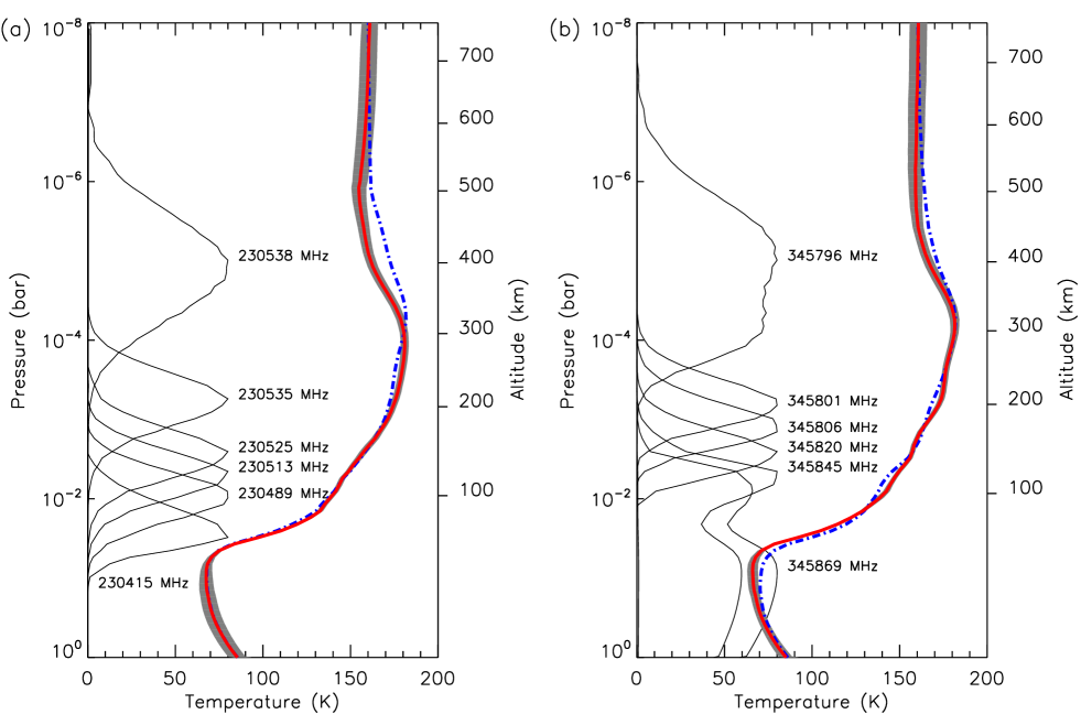
For the 2016 CO dataset (ALMA 2015.1.00512.S) the data were reduced in CASA Version 5.6.1-8 using the ALMA pipeline script prepared by the Joint ALMA Observatory staff, with the exception of the removal of the hifa_fluxcalflag task so that Titan’s atmospheric CO J=21 emission line at 230538 GHz was not flagged out. Data were deconvolved with the CASA clean task, using the Högbom algorithm with an image size = 128128 pixels, where pixels were set to 0.20.2. The resulting synthesized beam had FWHM (Full Width to Half Maximum) = 0.920.81, comparable to Titan’s angular size at the time of observing.
The data reduction of the 2017 data (2016.A.00014.S) has already been described in cordiner19. In addition, the bandpass solution interval was increased to 10 channels (2.44 MHz) to further improve the S/N and aid in the detection of weak spectral lines (Yamaki et al., 2012).
| Date | Start | End | * | Beam | Position | Angular | Sub-Earth | ||
|---|---|---|---|---|---|---|---|---|---|
| (UT) | (UT) | (mins) | (km s) | (MHz) | Size | Angle | Diameter () | Latitude | |
| Project Code 2015.1.00423.S | |||||||||
| 02-Mar-2016 | 09:44 | 10:57 | 43 | -28.37 | 24.13 | 0.870.75 | 89.145 | 0.71 | 26.28 |
| 02-Mar-2016 | 11:03 | 12:14 | 43 | -28.34 | 24.01 | 0.910.73 | 95.155 | 0.71 | 26.28 |
| 04-Mar-2016 | 09:43 | 10:55 | 43 | -32.18 | 27.37 | 0.870.64 | 79.815 | 0.71 | 26.28 |
| Project Code 2015.1.00512.S | |||||||||
| 01-Apr-2016 | 08:22 | 08:24 | 2 | -22.32 | 17.12 | 0.920.81 | -83.247 | 0.74 | 26.24 |
| Project Code 2016.A.00014.S | |||||||||
| 08-May-2017 | 08:49 | 09:07 | 18 | -19.28 | 22.24 | 0.180.15 | -80.950 | 0.77 | 26.41 |
| 16-May-2017 | 05:34 | 07:12 | 98 | -13.61 | 15.97 | 0.280.19 | -73.549 | 0.77 | 26.48 |
* Time spent on source.
Topocentric velocity (negative = approaching).
Frequency doppler shift (positive = blue-shifted).
| Spw | Freq. Range (MHz) | (MHz) | Molecule | (MHz) | Transition | |
| Project Code 2015.1.00423.S | ||||||
| 0 | 249570–250050 | 0.244 | 1920 | c-CHN | 249820 | =39, -band |
| 1 | 251260–251740 | 0.244 | 1920 | c-CHN | 251510 | =41, -band |
| 2 | 261900–262380 | 0.244 | 1920 | c-CHN | 262150 | =41, -band |
| 3 | 263090–263570 | 0.244 | 1920 | c-CHN | 263340 | =43, -band |
| Project Code 2015.1.00512.S | ||||||
| 4 | 230322 - 230791 | 0.244 | 1920 | CO | 230538 | 1 |
| Project Code 2016.A.00014.S | ||||||
| 5 | 344212-346085 | 0.977 | 1920 | CO | 345796 | 2 |
| 6 | 351281-352219 | 0.244 | 3840 | CHCN | — | multiple |
Channel spacing: spectral resolution is twice the channel spacing.
Disk-averaged spectra from all observations were extracted from an integrated region defined by a circular pixel mask set to contain 90% of Titan’s continuum flux, as in lai17.
3 Modeling
Modeling was accomplished using the NEMESIS program (irwin08), which has previously been successfully applied to model ALMA spectra of Titan (e.g. cordiner15; molter16; serigano16; palmer17; lai17; teanby18; thelen18; thelen19a; thelen19b). The NEMESIS fitting algorithm uses a Bayesian optimal estimation technique as described by rodgers00, which seeks to minimize a ‘cost function’ similar to a figure of merit, which penalizes the solution according to the square deviation of both the solution vector from the original a priori state, and also the model spectrum from the data. Marquart-Levenberg minimization is used to descend a downhill trajectory of the cost function until satisfactory convergence is reached (solution changing by 0.1%). ALMA spectra were rescaled to radiance units before being input to NEMESIS, and then modeled using a weighted average of spectra calculated at 35 emission angles from disk center to 1200 km altitude (3775 km radius), as described in teanby13, Appendix A.
Spectral line data for most molecules were taken from the CDMS catalog (muller01; muller05, https://cdms.astro.uni-koeln.de), which is a compilation of transition information from the published literature. These include: HCN (ahrens02; fuchs04; cazzoli05; maiwald00), CO (winnewisser97; goorvitch94), CHCN (kukolich73; kukolich82; boucher77; cazzoli06) , CHCN (muller08), c-CHN (kisiel99) and c-CH (bogey86; vrtilek87; lovas92), including their isotopes. The rotational spectrum of c-CHN was calculated by refitting the primary spectroscopic data from heineking86; wlodarczak88. For CHCN, we used a new, more complete spectral line list that included not only rotations in the ground vibrational state, but also in the first three vibrational states as described in kisiel20.
Collision-induced opacity for relevant molecular pairs was computed using published formalisms and publicly-available FORTRAN codes as follows: N–N (borysow86c); N–CH (borysow93); CH–CH (borysow87); N–H (borysow86a); CH–H (borysow86b); H–H (borysow91).
3.1 Temperature Retrievals
Firstly, the spectral lines of CO (Spw 4 & 5) were fitted using a model that allowed continuous variation of the temperature profile between 100–500 km, while CO was fixed at a constant mixing fraction of 49.6 ppm as determined by serigano16. The a priori temperature profile was constructed by interpolating measurements from the Huygens Atmospheric Structure Instrument (HASI) and Cassini radio science observations to Titan’s sub-observer latitude (26) below 100 km (fulchignoni05; schinder12), and disk-averaged retrieval results from 2015 ALMA observations of Titan (thelen18) were used at altitudes 100 km. Temperature a priori errors were set to 5 K in all atmospheric layers (0–1200 km), which allowed NEMESIS to obtain a fit to the data while limiting artificial vertical structure (ill-conditioning) in the retrieved temperature profile. Different frequency offsets from the line center sounded to different atmospheric depths (altitudes, or pressure levels), as shown by the contribution functions in Fig. 1. The a priori and final retrieved temperature profiles are also indicated.
3.2 Spectral windows 1 and 6: Discovery of Cyclopropenylidene
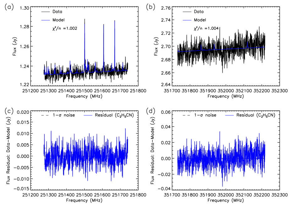
Next Spw 1111Window 0 was not included in this study. This region contains isotopic lines of CHCN, the analysis of which will be reported elsewhere. See also recent work on this isotopologue by iino20 was modeled to fit visible lines of known molecules: CHCN and CHCN. The temperature profile was fixed at the earlier retrieved profile from Spw 4 for 2016. Various gas profile types were investigated for the nitriles, adjusting the profiles to achieve best fits.
We first tried using minimalist ‘step’ functions (uniform volume mixing ratio above a fixed pressure level, and zero below) for the vertical distribution of each gas. From previous experience (e.g. cordiner15; lai17) we found that these worked well for trace (low abundance) nitriles in the ALMA spectrum where there is little information that can be obtained about the vertical profile. For CHCN we adopted a step altitude at 300 km. For CHCN, there was sufficient sensitivity to the altitude of the step to affect the quality of the fit, which was determined from Spw 1 and thereafter fixed at 250 km (see Appendix A). Initial fitting is shown in Fig. 2.
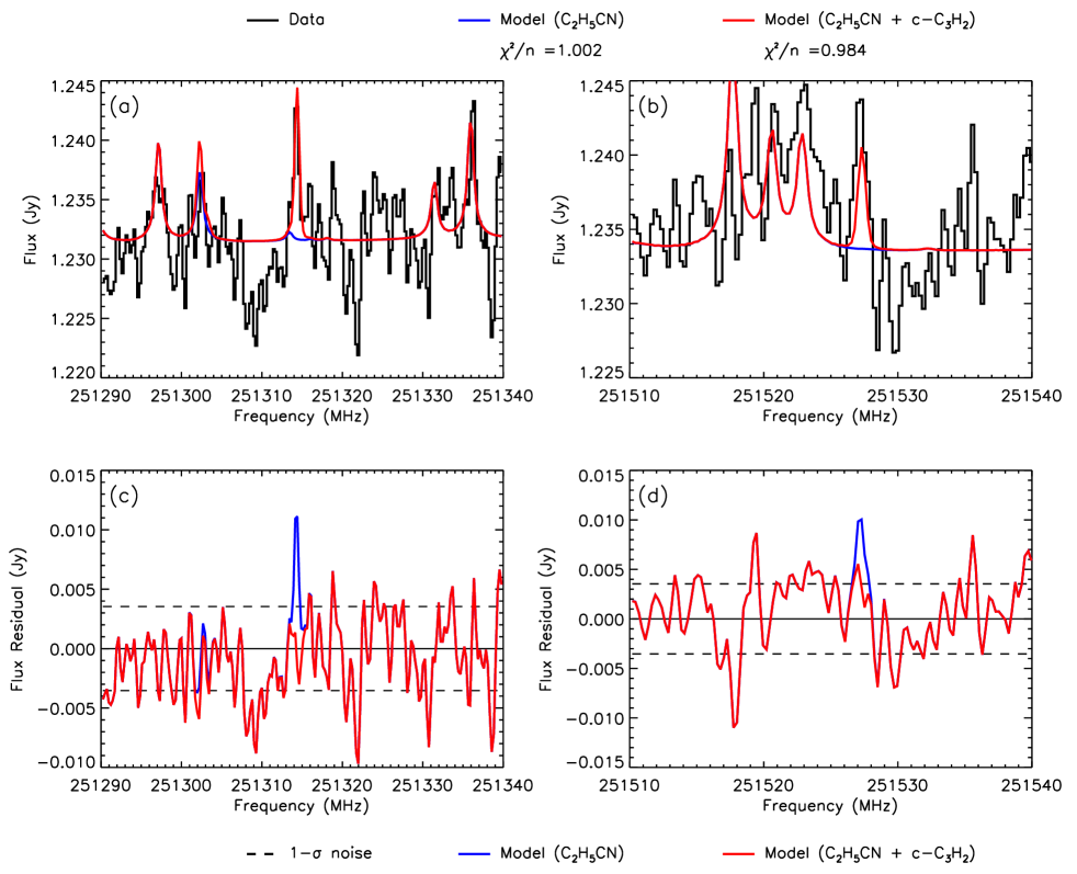
Having fitted the features of the known nitrile gases as well as possible, we proceeded to try adding additional gases to the model in an attempt to detect any weak lines due to a new species, including i-butanenitrile and n-butanenitrile (CHCN), propynenitrile (cyanodiacetylene, HCN) and others, using lines from the JPL catalog (pickett98, https://spec.jpl.nasa.gov). In both Spw 1 and 6, we found a significant improvement to the model fit after introducing the gas c-CH (cyclopropenylidene) using spectroscopic lines from CDMS originally determined by bogey86; vrtilek87 with a trial step function model with a step at 300 km, or higher.
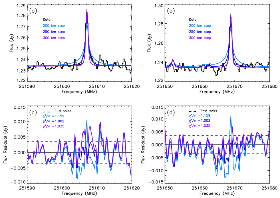
In Spw 1 two significant lines were detected at 251314.3 MHz (blend of and transitions) and 251527.3 MHz (), as shown in Fig. 3. We note that these two emissions are the strongest expected spectral features of c-CH in Spw 1, and show close to the expected proportions of relative intensities.
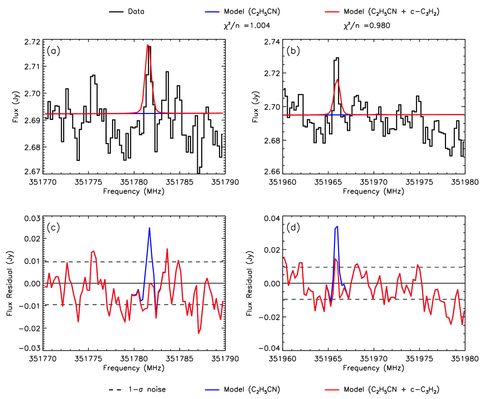
Similarly, in Spw 6, despite the noise level being higher in ALMA Band 7 than in Band 6 (Spw 1), we made two further detections of lines of c-CH: 351781.6 MHz (blend of the and doublet), 351965.9 MHz (blend of and doublet), see Fig. 4.
To further test the detection of c-CH, we calculated a curve for different amounts of the gas in a forward model, using a step function at 350 km. In this case, is a metric of spectral goodness-of-fit, where is the data spectrum, is the model spectrum, and is the spectral noise estimate. However, note that this is not the same definition as the more commonly used ‘reduced chi-square’ metric: , where is the number of spectral points minus the number of degrees of freedom (model parameters). In this case therefore a good fit occurs when (rather than ). We then define as the improvement to for various model trial abundances: , where denotes the best-fit model in absence of the trial gas, and is the same metric when an amount of the trial gas is present in the model (teanby09a; nixon10b; nixon13b; teanby18). An improved fit results in a that decreases below zero, and worsening fit results in that increases above zero.
Results are shown in Fig. 5. A strong minimum is seen for a volume mixing ratio ppb in Band 6, with reaching -21.24 indicating a =4.6 significance to the result. For Band 7, a minimum is reached at mole fraction ppb with -18.69 (4.3 ). Both results are significant, although the mixing ratio determined in each case is somewhat different (but consistent within error bars, as shown later in Section 4). The combined significance of the detection is 6.3 .

Retrieved abundances for c-CH with various profiles are described in Section 4.
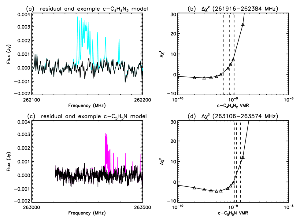
3.3 Spectral windows 2 and 3: Search for pyridine and pyrimidine
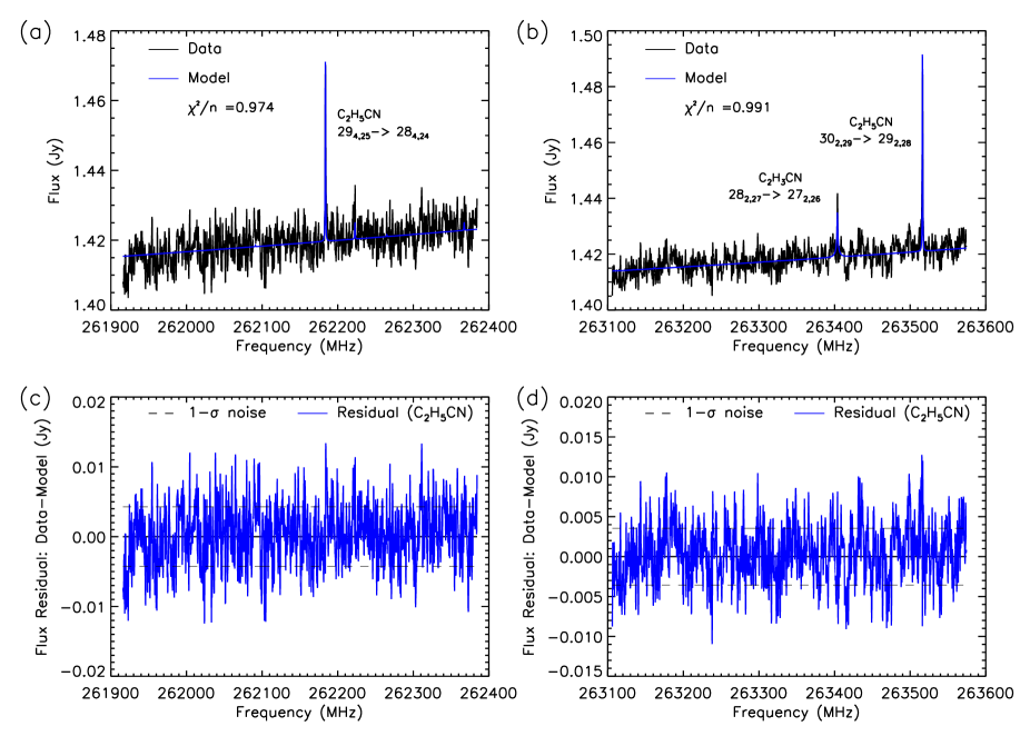
Fitting for Spw 2 & 3 was accomplished by initially using the retrieved temperature profile from Spw 4, and also scaling a 250-km step model for CHCN and 300=km step model for CHCN. In addition, we included HCN which contributed a continuum slope in these windows due to the wings of the strong 3 line at 265886 MHz whose line center lies outside the bandpass. Then, 300-km step model profiles models for c-CHN (Spw 2) and c-CHN (Spw 3) were introduced, but resulted in no significant improvement to the fit as measured by a reduced test. Instead, upper limits for c-CHN and c-CHN were determined instead (see Section 4.) The final fit for these spectral windows is shown in Fig. 6.
4 Results
4.1 Retrieval errors
The propagation of errors in the retrieval process follows the formalism described in irwin08, and further elaborated in Section 3.5 of nixon08a (hereafter N08). This includes a combination of a priori and measurement error (Eq. 1 of N08), with the error from the earlier temperature propagated as additional measurement error (Eq. 2 of N08). In addition, we needed to make a further error allowance for apodization, which reduces independent information in the spectrum. Due to the Hanning apodization applied during the Fourier Transform, neighboring spectral channels become correlated, and the signal-to-noise in our retrieval will be overestimated by a factor equal to the square root of the number of channels per resolution element - two channels per resolution element for Hanning apodization. At the same time, there is a small gain of 1.095 from averaging information across two successive correlated channels222ALMA technical notes: https://help.almascience.org/index.php?/Knowledgebase/Article/View/29, so the final error bars are increased by a factor . This factor has also been applied to correspondingly reduce the detection significances ( levels) throughout the paper.
4.2 Cyclopropenylidene
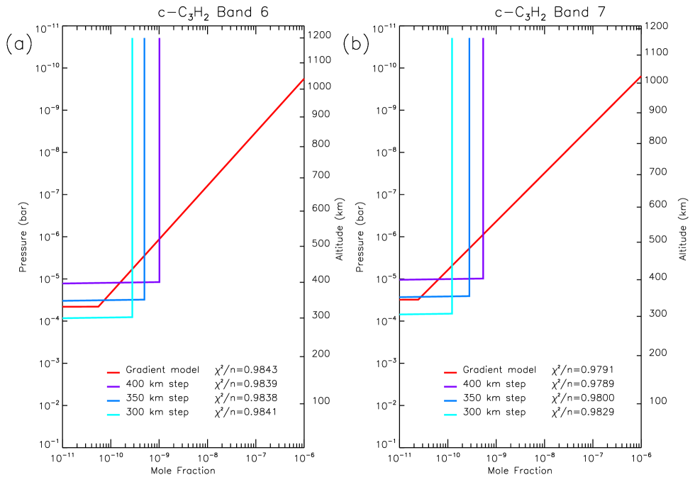
We initially fitted the c-CH emissions with a step function model, where the gas abundance was zero below a ‘step’ altitude and a uniform value above. The overall profile was then scaled to achieve a best fit. The effect of changing the altitude of the step was also explored, since lower steps increased pressure broadening of the lines that became greater than the observed line widths.
We also investigated a more realistic gas profile, with an abundance decreasing downwards to a condensation altitude, by using a four-parameter gradient model. This model was defined by two (pressure, mixing ratio) co-ordinates defining a straight-line, logarithmically decreasing VMR between (upper point) and (lower point). Above the VMR was assumed constant at and below the VMR dropped to zero. The upper pressure level was set to be bar, or approximately 1100 km, the altitude of the INMS measurements of the CHH (protonated) ion. The initial value for the abundance at this altitude was set to be in line with the INMS ion measurements (vuitton07). The initial value for the lower point was set to be: bar, , a pressure level corresponding to approximately 300 km, and allowing a lenient variation of abundance.
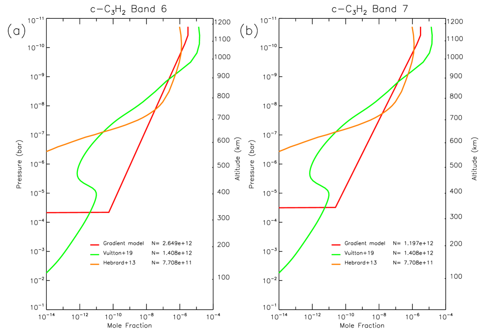
Scaled step function solutions for c-CH from Window 1 (Band 6) and Window 6 (Band 7) are shown in Fig. 7, along with best fit gradient model profiles. Numerical results are given in Table 3. Retrievals for cyclopropenylidene showed low sensitivity to the altitude of the step, with a weak minimum at 300–400 km. The resulting abundances and columns were slightly different in 2016 and 2017. For a step function of 350 km we obtained a VMR of 0.50 0.14 ppb and column abundance of 3.5 cm in 2016, but somewhat lower VMR (0.28 0.08) and column abundance (1.5) in 2017. This implies either (a) that the global abundance had decreased from 2016 to 2017, or, (b) if the real abundance was constant, then a mean value of 0.33 0.07 ppb for the 350 km step profile.
| Band | Species | Model | /n | VMR | Col. Abund. |
|---|---|---|---|---|---|
| (ppb @ 600 km) | (molecule cm) | ||||
| 6 | c-CH | Gradient model | 0.9843 | 3.788 | 2.649 |
| 6 | c-CH | 400 km step | 0.9839 | 1.012 0.386 | 2.824 |
| 6 | c-CH | 350 km step | 0.9838 | 0.495 0.142 | 3.487 |
| 6 | c-CH | 300 km step | 0.9841 | 0.278 0.054 | 4.875 |
| 7 | c-CH | Gradient model | 0.9791 | 1.867 | 1.197 |
| 7 | c-CH | 400 km step | 0.9789 | 0.537 0.223 | 1.175 |
| 7 | c-CH | 350 km step | 0.9800 | 0.279 0.084 | 1.541 |
| 7 | c-CH | 300 km step | 0.9829 | 0.122 0.031 | 1.702 |
Retrieved parameters for the gradient model retrievals in 2016 and 2017 are shown in Table 4, along with parameters for a weighted mean profile of both years.
| (bar) | (bar) | |||
|---|---|---|---|---|
| Band 6 | ||||
| a priori | (5.02.0) | (3.41.0) | (1.00.5) | (2.01.9) |
| Retrieved | (4.42.2) | (3.11.2) | (4.72.9) | (5.43.7) |
| Band 7 | ||||
| a priori | (5.02.0) | (3.41.0) | (1.00.5) | (2.01.9) |
| Retrieved | (4.32.2) | (3.11.2) | (3.82.3) | (2.11.7) |
| Band 6 & 7 | ||||
| Combined | (4.31.6) | (3.10.8) | (4.11.8) | (2.61.5) |
4.3 Pyridine and pyrimidine
Upper limits for c-CHN and c-CHN were determined using the method outlined for c-CH in Section 3.2. In this case, the 1, 2 and 3- upper limits are indicated at the trial abundances where the reaches +1, +4, and +9 respectively (nixon12b). Results are shown in Fig. 8 and Table 5. A shallow minimum was detected for c-CHN, however the spectrum does not show obvious emissions consistent with expected spectral lines, therefore we believe this to be likely due to random spectral noise (although worthy of a more sensitive follow-up observation to be sure).
| Name | p (bar) | Freq. (MHz) | NEF (mJy) | 1- VMR | 2- VMR | 3- VMR |
|---|---|---|---|---|---|---|
| c-CHN | 0.020 | 262143 | 0.34 | 0.663 | 0.854 | 1.042 |
| c-CHN | 0.020 | 263331 | 0.29 | 1.046 | 1.153 | 1.356 |
Noise Equivalent Flux. Volume Mixing Ratio (mole fraction) in ppb.
5 Discussion
5.1 Cyclopropenylidene
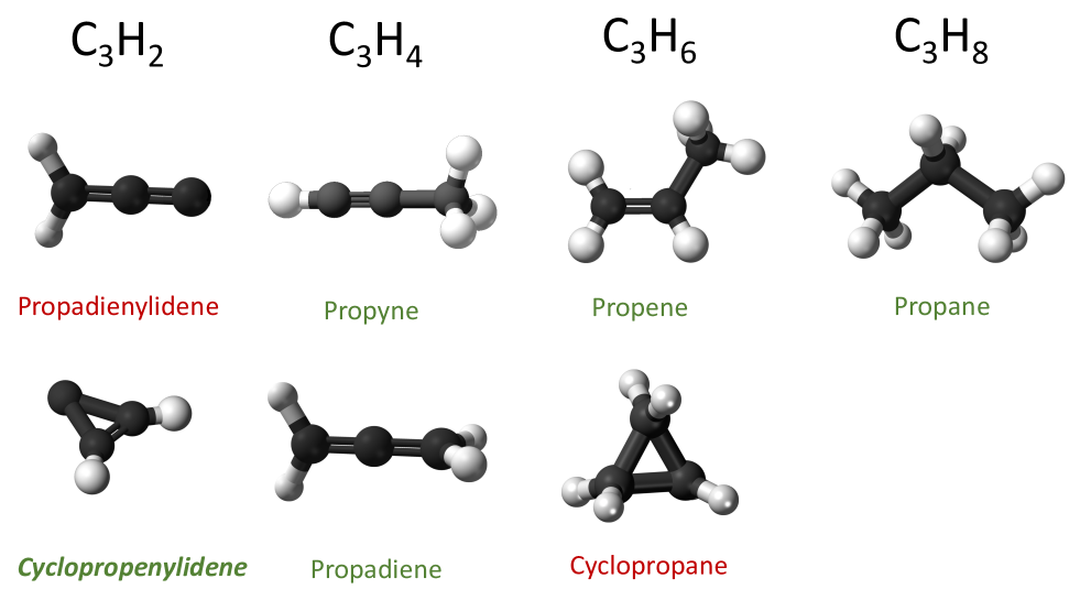
The molecule cyclopropenylidene (c-CH) was discovered in the interstellar medium (ISM) by thaddeus85 through extensive laboratory and theoretical analysis to unearth the origin of several prominent, but previously unidentified lines seen on radio astronomical spectra. Following this discovery, the molecule has been found to be ubiquitous in the galaxy (fosse01) and easily detectable due to the relatively large dipole of 3.43(2) D (kanata87) caused by the unpaired electrons on the bivalent carbon atom. In addition, c-CH is a light molecule with a small partition function, which also works in favor of detection. One of its linear isomers, propadienylidene (HCCC, see Fig. 9) has since been detected in the ISM (cernicharo91) while propynylidene (HCCCH) has not been observed. Note that propadienylidene is higher in energy than cyclopropenylidene, and therefore metastable, so that the observed ratio of ten or more for c-CH/HCCC is expected.
The Cassini INMS instrument measured peaks at 38 and 39 in samples of Titan’s upper atmosphere that were attributed to the presence of CH and various isomers of CH (vuitton06a; vuitton07). Although the molecular structure was not directly measurable, modeling of the mass spectrum implied ion number densities of 0.0016 cm (CH), 34 cm (c-CH) and 1.6 cm (l-CH) respectively. Determining the ratio of l-CH/c-CH was deemed to be of major importance by vuitton07 (and the subject of laboratory investigation), since the linear propargyl ion is able to react to form heavier species, including possibly benzene (wilson04), while the cyclopropenylidene ion is essentially a terminal species, leading to c-CH.
Various mechanisms have been proposed for the formation of c-CH and it is not clear at present which mechanisms are the most important. In the original work of thaddeus85 on the ISM detection, cyclopropenylidene was produced by dissociative electron recombination of the cyclopropenylium cation, c-CH:
| (1) |
while c-CH is produced from CH in two steps. First the fast ion-molecule reaction:
| (2) |
followed by the slower radiative association (hydrogenation):
| (3) |
Alternatively the CH ion has been proposed to be produced from acetylene via many other possible ion molecule reactions by vuitton19, for example:
| (4) |
| (5) |
walch95; guadagnini98 investigated the reactions of CH() (methylidyne) with CH, predicting that various isomers of both CH and CH can result. From this point, several outcomes are possible: the products can stabilize into a less-reactive species, such as c-CH, or else can undergo further reactions to form heavier hydrocarbons. In particular, it was noted that both CH and CH can dimerize, forming benzene (CH) and -benzene (CH) respectively, and therefore CH and CH are important stepping stones to polycyclic aromatic hydrocarbons (PAHs).
The work of canosa97 further clarified pathways to formation of CH from reactions of the methylidine radical (CH) with unsaturated CH hydrocarbons, such as:
| (6) |
| (7) |
In the above reactions, CH is envisaged to add to the carbon-carbon double or triple bond. CH can be converted to CH by hydrogen loss through photodissociation (e.g. hebrard13):
| (8) |
The CH radical may also result from the methylidine insertion reactions, which can lead to CH via several steps, first charge transfer:
| (9) |
followed by hydrogenation (3) and then dissociative recombination (1) as before. Subsequently, canosa07 showed that C reactions may also be important, e.g,:
| (10) |
as used in the photochemical model of krasnopolsky09. The branching ratios between aliphatic and aromatic pathways in many of these reactions, especially at low temperatures, are important and often poorly known.
In Fig. 10 we compare our retrieved gradient models to photochemical model predictions of hebrard13 and vuitton19. In fact, the models arrive at a column abundance rather similar to our retrieved amount of 10 cm . It is difficult to pronounce whether the differences in the vertical profile shape are significant or not, since we have very little constraint on this at present.
5.2 Pyridine and pyrimidine
The astrobiologically important species pyridine (c-CHN) and pyrimidine (c-CHN) are nitrogen-containing heterocyclic ring molecules resembling a benzene ring with either one or two of the C-H members replaced by a nitrogen atom. Pyrimidine in particular is of significant biological importance since it forms the backbone ring structure of several key biological molecules - specifically the nucleobases uracil (in RNA), cytosine (in RNA and DNA) and thymine (in DNA). These molecules can potentially be formed from pyrimidine after the chemical substitution of functional groups (-NH, -CH and =O) in place of hydrogen, as indicated in Fig. 11. Indeed, laboratory experiments (nuevo14) have shown that UV irradiation of pyrimidine in the presence of HO, CH, CHOH and NH can form uracil and cytosine - but not the more complex thymine - a possible clue as to why thymine appears only in DNA but not RNA, and further evidence that RNA may have preceded DNA. Similar processes may be taking place in space, including the atmosphere of Titan. Indeed, laboratory simulations of Titan’s atmosphere, using multiple experimental techniques such as GC-MS (gas chromatograph mass spectroscopy), pyrolysis mass spectroscopy, Raman and reflectance spectroscopy etc have been successful in positively identifying the nitrogen heterocycles (khare84b; ehrenfreund95).
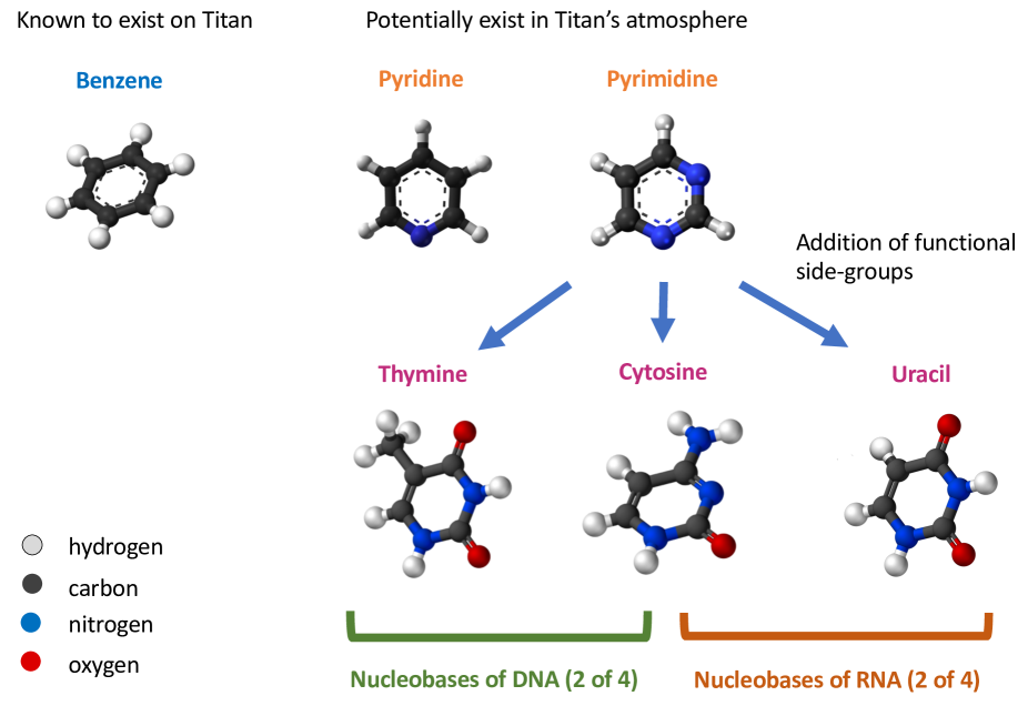
To date, neither pyridine nor pyrimidine have been detected in astrophysical sources, despite searches in molecular clouds (simon73; kuan03; kuan04; cordiner17; mcguire18) and in the envelopes of evolved stars (charnley05), although pyridine and quinoline (2-membered N-heterocycle rings) derivatives have been found in meteorite samples (e.g. stoks82; martins18). peeters05 have shown that these molecules are relatively unstable against UV irradiation compared to benzene, but could survive for 10–100s of years in dense clouds where UV flux is attenuated, and therefore potentially in Titan’s thick atmosphere.
The potential presence of the nitrogen heterocyclic molecules pyridine and pyrimidine in Titan’s atmosphere may be inferred from the detection of CHNH and CHNH ions in Cassini mass spectra (vuitton07) at 80 and 81 (seen in their Fig. 2). As with the hydrocarbons, the elucidation of structure from the mass spectra alone is not possible, therefore for example protonated forms of branched acyclic molecules such as penta-2,4-dienenitrile or 2-methylene-3-butenenitrile could be responsible for the mass 80 peak instead.
Formation pathways for the N-heterocycles are currently quite uncertain. For example, fondren07 suggest that efficient ion-molecule association reactions with HCN could form pyridine and pyrimidine from smaller ions:
| (11) |
| (12) |
A more exotic mechanism for the formation of pyridine through ring expansion of pyrrole by methylidyne has been observed in the gas phase by soorkia10:
| (13) |
More recently, balucani19 has investigated a pathway to pyridine that begins with an attack on CH by N(D), leading to a chain of unstable intermediate products that may decay to c-CHN.
The relative importance of these various channels is highly uncertain at the present time, leading to difficulties in incorporating these molecules into photochemical models. For example krasnopolsky09 included just one hypothetical formation pathway for pyridine by the radical-molecule reaction:
| (14) |
while in (loison15) only the aliphatic isomer CHCN is discussed.
Our analysis indicates 2- upper limits of ppb and ppb for c-CHN and c-CHN respectively (constant profile above 300 km), which may in future be used to place some constraints on photochemical models as these become more sophisticated and add more detailed treatment of cyclic molecule formation.
6 Conclusions
We report the first detection of c-CH (cyclopropenylidene) on Titan in two datasets: Band 6 spectra from 2016 and Band 7 data from 2017, detecting at least 2 emissions in each case. The derived abundances are 0.50 0.14 ppb in 2016 and 0.28 0.08 in 2017 for a 350-km step model, which are in agreement at the margins of their 1- errors, or alternatively may indicate a real decrease in abundance. Derived column abundances are 3–5 cm in 2016 and 1–2 cm in 2017, in good agreement with photochemical models. This presence of cyclopropenylidene is of substantial significance to Titan’s atmospheric chemistry, since insertion reactions of methylidyne (CH) into CH and other unsaturated hydrocarbons can lead to formation of CH and CH isomers. These in turn may be stepping stones to benzene and -benzene, and larger aromatic PAH molecules.
Following preliminary evidence from Cassini mass spectra, we also searched for the N-heterocyclic molecules pyridine and pyrimidine in Titan’s atmosphere, with a null result. By modeling of ALMA spectra at 262–263 GHz we have determined 2- upper limits of 1.15 and 0.85 ppb for c-CHN and c-CHN respectively. We have detected ground state lines of CHCN and CHCN as previously seen in Titan’s atmosphere, and also vibrationally excited rotational transitions of CHCN. The CHCN emissions are well-fitted using a 250 km ‘step’ model as noted by previous authors, and we find a best-fit abundance of 5.0 0.1 ppb similar to previous work. Our modeling indicates that there is unlikely to be substantial amounts of CHCN below 250 km, in contrast to existing photochemical models.
The discovery of cyclopropenylidene for the first time in a dense planetary atmosphere therefore opens up new directions for research in the chemistry of the reducing atmospheres of the outer planets, and especially PAH and haze formation.
Appendix A Propionitrile
A.1 Modeling
In Spw 1, sufficiently strong lines of CHCN were seen that there was noticeable pressure-induced line broadening, allowing an optimum altitude for a step function model to be determined. Fig. 12 shows the effect of changing the step function altitude for CHCN.
The goodness of fit for all models is compared in Table 6. The best-fit solution for CHCN is a step function at 250 km with a uniform VMR of 5.0 0.07 ppb and column abundance 2.2 cm. A comparison of retrieved profiles can be seen in Fig. 13(a).
| Species | Model | VMR | Col. Abund | |
|---|---|---|---|---|
| (ppb @ 600 km) | (molecule cm) | |||
| CHCN | Gradient model | 1.051 | 31.957 | 1.3475 |
| CHCN | 300 km step | 1.035 | 8.545 0.252 | 1.5004 |
| CHCN | 250 km step | 1.002 | 5.040 0.095 | 2.2378 |
| CHCN | 200 km step | 1.159 | 2.749 0.030 | 3.5703 |
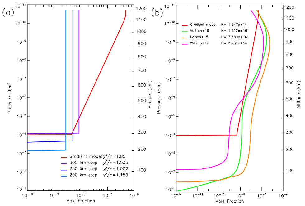
A gradient model was also tested, using similar initial conditions to those used for c-CH, as described in Section 3.2, except that the initial abundance at the 1100 km altitude was set to in line with the INMS measurement of CHCNH. Initial and retrieved parameters for the CHCN gradient model are given in Table 7.
| Gas | (bar) | (bar) | |||
|---|---|---|---|---|---|
| CHCN | a priori | ||||
| CHCN | Retrieved |
A list of the ground-state and vibrationally excited lines detected in Spw 1 is given in Table 8.
| Species | Freq. (MHz) | Transition | (K) | |
|---|---|---|---|---|
| CHCN | 251271.3 | - | 0 | 240 |
| CHCN | 251278.7 | - | 0 | 533 |
| CHCN | 251284.2 | - | 2 | 776 |
| CHCN | 251289.1 | - | 1 | 624 |
| CHCN | 251297.1 | - | 1 | 600 |
| CHCN | 251302.3 | - | 1 | 651 |
| CHCN | 251331.4 | - | 1 | 680 |
| CHCN | 251335.9 | - | 1 | 577 |
| CHCN | 251365.8 | - | 0 | 573 |
| CHCN | 251373.2 | - | 1 | 712 |
| CHCN | 251404.3 | - | 3 | 751 |
| CHCN | 251409.4 | - | 3 | 751 |
| CHCN | 251419.7 | - | 1 | 557 |
| CHCN | 251425.6 | - | 1 | 744 |
| CHCN | 251459.0 | - | 0 | 616 |
| CHCN | 251487.2 | - | 1 | 780 |
| CHCN | 251501.0 | - | 0 | 203 |
| CHCN | 251517.7 | - | 1 | 539 |
| CHCN | 251520.6 | - | 2 | 524 |
| CHCN | 251522.9 | - | 2 | 524 |
| CHCN | 251558.1 | - | 0 | 661 |
| CHCN | 251560.2 | - | 1 | 509 |
| CHCN | 251561.2 | - | 1 | 509 |
| CHCN | 251570.0 | - | 0 | 253 |
| CHCN | 251607.1 | - | 0 | 202 |
| CHCN | 251652.3 | - | 2 | 511 |
| CHCN | 251661.0 | - | 0 | 41 |
| CHCN | 251668.8 | - | 0 | 193 |
| CHCN | 251691.0 | - | 3 | 739 |
| CHCN | 251713.6 | - | 2 | 511 |
| CHCN | 251728.7 | - | 0 | 41 |
Rotational energy levels are labeled with , and omission of identifies a degenerate spectroscopic doublet in which and .
Vibrational species: 0: ground state (brauer09), 1: (kisiel20), 2: (kisiel20), 3: (daly13).