Probabilistic Programming with CuPPL

Abstract.

Probabilistic Programming Languages (PPLs) are a powerful tool in machine learning, allowing highly expressive generative models to be expressed succinctly. They couple complex inference algorithms, implemented by the language, with an expressive modelling language that allows a user to implement any computable function as the generative model.

Such languages are usually implemented on top of existing high level programming languages and do not make use of hardware accelerators. PPLs that do make use of accelerators exist, but restrict the expressivity of the language in order to do so.

In this paper, we present a language and toolchain that generates highly efficient code for both CPUs and GPUs. The language is functional in style, and the toolchain is built on top of LLVM. Our implementation uses delimited continuations on CPU to perform inference, and custom CUDA codes on GPU.

We obtain significant speed ups across a suite of PPL workloads, compared to other state of the art approaches on CPU. Furthermore, our compiler can also generate efficient code that runs on CUDA GPUs.

1. Introduction

Probabilistic Programming Languages (PPLs) are a powerful machine learning tool, allowing highly expressive generative models to be expressed succinctly, and complex inference to be applied to them. They typically provide a range of built-in distributions from which samples can be drawn and scored, along with a range of inference algorithms.

CuPPL is a functional programming language, with all of the standard control flow constructs including let expressions, conditional expressions, recursive functions, algebraic datatypes and case statements. It also includes a vector data type and a suite of built-in vector operators such as map, reduce and repeat. CuPPL provides two basic probabilistic primitives: sample and factor. These can be used within a generative model to sample from and score a suite of built-in distributions and user defined distribution objects. These primitives are implemented in using delimited continuations and the operators shift and reset (Felleisen, 1988). CuPPL then provides inference methods that can be applied to a model function in order to generate the posterior distribution from the model.

1.1. PPL Example

An example of a generative model is given in Figure 1, which demonstrates the diverse control flow that CuPPL allows within the model function, and which gives PPLs their expressive power.

This model finds the $n$-degree polynomial that best fits some given data. The degree of the polynomial is sampled from a uniform prior, and its coefficients from gaussian priors. The polynomial is then conditioned on a measure of its “distance” from the data. The model returns the polynomial, as a vector of coefficients. Running inference on this model produces an empirical distribution over polynomials, and the mode of this distribution is the “line of best fit” for the data.

⬇

model <- function() {

n <- sample(uniform-discrete(2,5));

line <- repeat(

function(i) { sample(normal(0,10)) },

n);

factor(-distance(line, data));

line

}

Figure 1. An example program that demonstrates the use of universal language features in a model function. The implementation of distance is omitted for brevity.

1.2. Delimited Continuations

Whenever the model function calls sample or factor, or returns a value, the inference algorithm needs to make decisions about its execution – more specifically the probability of a trace of execution through the model needs to be tracked and samples need to be generated.

We use delimited continuations (the shift and reset operators) to allow the inference algorithm to manipulate the execution of the model function and generate samples from its posterior distribution.

shift(k, e) captures the current state of the program up to the last enclosing reset(.), creates a function from this that can be called via $k$, and evaluates $e$. $e$ may call $k$ as few or as many times as it likes.

Using shift whenever sample or factor are called captures the current state of execution of the model function (up to the start of the execution of the model function) and allows the inference algorithm to decide what to execute next.

Section 3 describes our implementation of sample and factor in more detail.

1.3. Contributions

In this paper, we make the following contributions:

• We describe a probabilistic programming language that is functional in nature, and supports delimited continuations using the shift and reset operators described in (Asai and Kameyama, 2007). The language uses answer type polymorphism in its type system to statically type check the code enabling statically typed LLVM IR to be generated from it.

• A novel implementation strategy for delimited continuations in LLVM IR that enables inference to be implemented in LLVM IR in a similar style to that described in (Goodman, 2013).

• The code generated by our compiler performs significantly better than both Anglican (Tolpin et al., 2016) and webppl (Goodman and Stuhlmüller, 2014) over a range of benchmark programs.

• Moreover, the code generated by our compiler also scales well to large numbers of samples.

1.4. Structure

The rest of the paper is structured as follows. In Section 2 we discuss related work, in Section 3 we give an overview of the features and type system CuPPL, and in Section 4 we discuss the design and implementation of the code generator. This is followed in Section 5 by a performance analysis of our language across a range of benchmarks, comparing against both webppl (Goodman and Stuhlmüller, 2014) and Anglican (Tolpin et al., 2016). Section 6 concludes the paper.

2. Related Work

The probabilistic programming languages most similar to our own are Anglican (Tolpin et al., 2016) and webppl (Goodman and Stuhlmüller, 2014), however both of these languages are embedded in other programming languages. The semantics of our language also borrows heavily from (Goodman, 2013) which describes many of the principles behind implementing probabilistic languages.

Anglican (Tolpin et al., 2016) is embedded in Clojure (clo, 2018), a dialect of Lisp that works in the Java Virtual Machine. In is built on top of continuations and trampolines in order to capture control and pass it to the inference algorithm.

webppl (Goodman and Stuhlmüller, 2014) is written in Javascript, on top of the NodeJS ecosystem (nod, 2018). It uses coroutines to capture control and pass it to the inference algorithm.

Similarly to Anglican and webppl, Kiselyov et al (Kiselyov and Shan, 2009) describe a domain specific probabilistic language that is embedded in OCaml. They also use the delimited continuation approach to explore programs as models.

Edward (Tran et al., 2016, 2017) is a probabilistic modelling library for TensorFlow (Abadi et al., 2015). This is not a true PPL as it does not allow arbitrary control flow, and is limited by the graph structures that are representable in TensorFlow.

Compiler based techniques to producing PPL code include (Wingate et al., 2011). This approach translates a PPL problem into MCMC code, rather than compiling the model function in the language itself. TerpreT (Gaunt et al., 2016) is a domain specific probabilistic language for program induction, generating programs from a PPL model.

Earlier approaches to probabilitic programming and modelling include BUGS (Lunn et al., 2009), which is restricted to Bayesian modelling and cannot handle the complex control structure that true PPLs can.

Stan (Carpenter et al., 2017), similarly to BUGS, is restricted to Bayesian modelling. Bindings exist for embedding Stan in either R or Python. Other early, and similar, approaches include Church (Goodman et al., 2012).

Borgstrom et al (Borgström et al., 2016) present a rigorous lambda calculus for probabilistic programming, in the style of CuPPL, Anglican, webbpl and Church. They use this to prove that they perform MCMC inference on program traces correctly.

3. The Language

CuPPL is a statically-typed functional language, and its design is centered around vectors and data parallel operations. It is also designed to allow high-level language transformations such as deforestation of vector operations, closure conversion and other high level optimization passes.

The rest of this section is structured as follows. Section 3.1 describes the salient features of CuPPL. Section 3.3 describes how delimited continuations are expressed, Section 3.4 details how these are used to implement sample and factor, and finally Section 3.5 details how the polymorphic type system treats delimited continuations using answer types.

3.1. Language Features

CuPPL includes the usual control flow constructs you would expect from a functional language including lambda expressions, let-expressions, conditionals, case statements and recursion. The language also includes first class vector data types of arbitrary dimensions, and a suite of parallel operators that work over them, including:

• map applies a function to every element of the vector

• repeat generates a vector by running a function a given number of times

• reduce performs a parallel reduction over a vector

• filter constructs a new vector that includes only those elements from the input vector for which a given predicate returns true

3.1.1. Type Generalization and Specialization

CuPPL allows type generalization and specialization, in a similar manner to System F. Polymorphic types can be defined as follows:

⬇

type List ’a :

(+ (Nil : unit)

(Cons : (’a, (List ’a))));

This example demonstrates both type generalization and type specialization. List is the type constructor:

⬇

forall ’a .

(+ (Nil : unit)

(Cons : (’a, (List ’a))))

This type can be specialized to store a list of integers by using a type application:

⬇

(List int)

This produces the concrete type:

⬇

(+ (Nil : unit)

(Cons : (int, (List int))))

We impose a few restrictions on the use of generalized types, forall types and type applications. Firstly, general types can only be constructed at the start of a module, as the type constructors need to be unique within a module. Secondly, after type checking a program, all types must be specialized, or turned into concrete types. This is because the LLVM IR target environment requires all types to be concrete. If an expression is discovered whose type is not specialized to a concrete type (such as partial application of a parallel operator), the compiler complains that it could not statically determine the concrete type of the expression.

3.2. Distribution Values

The type system includes a distribution type, denoted ~t which is a distribution over values of type t. It also includes a suite of built-in distributions, including gaussian, bernoulli, poisson and many others. Built-in functions to perform operations on distribution values are also provided, such as sample* which produces a sample from a distribution, dist-score which scores a sample from a distribution and dist-var which returns the variance of a distribution.

3.3. Delimited Continuations

CuPPL allows delimited continuations through the use of the shift and reset constructs (Felleisen, 1988; Asai and Kameyama, 2007).

Informally, the meaning of shift is to capture the current execution state up to the last reset, wrap it in a function, and bind a name to that function.

For example, consider the following:

⬇

reset(1 + shift(k, k(2)))

When shift is encountered, it captures the current program as a function named $k$. In this case $k$ is:

⬇

function (x) { 1 + x }

It then executes the body of the shift expression, which executes k(2), so the program returns 3.

Reset limits the scope to which shift will capture the state of the program. For example, consider the following:

⬇

1 + reset(3 + shift(k, 1))

When shift is encountered, it captures the current program as a function $k$ up to the last reset. In this case $k$ is:

⬇

function (x) { 3 + x }

It then executes the body of the shift expression, which simply returns 1 and does not execute $k$, so the program returns 2 as its result.

3.4. Inference, sample and Factor

The two basic PPL primitives sample and factor are expressed in terms of delimited continuations. Figure 2 gives the definition of sample and factor (and the observe helper function) in terms of shift and reset.

⬇

sample <- function (dist : ~a) : a {

shift (k : a => b) {

x <- sample-impl(dist, k);

(x[0])(x[1])

}

}

⬇

factor = function (log-p : a) : unit {

shift k {

f <- factor-impl(log-p, k);

f()

}

}

⬇

observe = function (dist, x) : unit {

factor(dist-score(dist, x))

}

Figure 2. Implementation of sample, factor and observe using delimited continuations

sample uses the shift operator to capture the current execution state of the model function as a function $k$. When inference starts, reset is called to limit the scope of this capture up to the start of the execution of the model function. sample then calls sample-impl with the distribution object that was sampled from and $k$. The implementation of sample-impl depends on the choice of inference algorithm, however it always returns a tuple of type (a => b, a). This function represents what the program should do next: the first element of the tuple is a continuation, with the same type as $k$, and the second element of the tuple is a sample from the distribution, of type a.

factor also uses shift operator to capture the current execution state of the model function as a function $k$. It then calls factor-impl with the log probability with which to update the program trace. The implementation of sample-impl depends on the choice of inference algorithm, however it always returns a function of type unit => unit. This is a function denoting what the program should do next, and has the same type as $k$.

observe is a wrapper function around factor that makes altering the log probability of the execution trace based on observing data from a distribution simpler. It calls factor with the score of the given sample x from the given distribution dist.

CuPPL provides two inference methods that implement sample-impl and factor-impl. They are invoked via built-in functions called importance (for running importance sampling) and mcmc (for running Monte Carlo Marov Chain based inference. More details on the implementation of these functions can be found in Section 4.

3.5. Type System

CuPPL uses Hindley-Milner type inference, augmented with polymorphic answer types (Asai and Kameyama, 2007). Figure 3 gives a subset of the type rules. Te following notation is used:

• Types are denoted $\tau$.

• Type schemes are denoted $\sigma$. They have the syntax $\sigma=\tau\mid\forall A.\tau$ where $A$ is a set of type variables.

• $\tau\prec\sigma$ denotes that type $\tau$ is an instance of type scheme $\sigma$

• Answer types are denoted $\alpha$, $\beta$, $\gamma$. Answer types can be any type $\tau$ or the empty type, denoted $\bot$

• Expressions are denoted $e$.

• Constant values are denoted $c$.

• Variable identifiers are denoted $x$.

• Type environments are denoted $\Gamma$. These map variable identifiers $x$ to type schemes $\sigma$. The notation $\Gamma\{x:\sigma\}$ denotes mapping $\Gamma$ updated with identifier $x$ mapped to type scheme $\sigma$. $\Gamma_{0}$ denotes an empty type environment, that does not map any identifiers to type schemes.

• There are two forms of type judgements:

  • Pure type judgments are written $\Gamma\vdash_{p}e:\tau$. This means that expression $e$ has type $\tau$, given type environment $\Gamma$.

  • Impure type judgments are written $\Gamma,\alpha\vdash e:\tau,\beta$. This means that expression $e$ has type $\tau$, given type environment $\Gamma$ and the execution of $e$ changes the answer type from $\alpha$ to $\beta$.

(

lambda) &Γ{x : τ_1}, α_1 ⊢e : τ_2, α_2Γ⊢_p function [α_1 α_2] ( x : τ_1 ): τ_2 { e } : τ_1 / α_1 →τ_2 / α_2
(apply) Γ,α_1 ⊢e_1 : τ_2 / α→τ/ α_2, βΓ,α_2 ⊢e_2: τ_2,α_1Γ,α⊢e_1 ( e_2 ) : τ,β
(reset) Γ,α⊢e : α,τΓ⊢_p reset { e } : τ
(shift) Γ{x : ∀t.( τ/ t →α/ t )}, τ_2 ⊢e : τ_2,βΓ,α⊢shift (x : τ_1) : τ_2 { e } : τ,β
(expr) Γ⊢_p e : τΓ,α⊢e : τ,α

Figure 3. Subset of the type rules for CuPPL.

The expr rule allows an expression with the same input and output answer types to be type checked as a pure expression.

3.6. Inference Methods

CuPPL supports three inference methods.

3.6.1. Enumeration

Enumeration performs precise inference on the model function, by executing all possible paths through the function. The probabilistic branching points are when the model calls sample. Whenever sample is called, the inference algorithm executes the model function from that point for all values in the support of the distribution. This only works for distributions with finite support, and returns a runtime error if a continuous distribution is encountered. This performs a breadth first traversal through the model function, and the depth of this traversal can be limited to a maximum depth if desired.

3.6.2. Importance Sampling

This performs importance sampling (Ripley, 2008) on the model function. This is done by repeatedly running the model function. The calls to sample and factor made by each execution prescribe a log probability the value returned by the model function. The model function is repeated up to a chosen number of times, and the posterior distribution is computed by normalizing the log probabilities of the returned values.

3.6.3. Lightweight Metropolis-Hastings

This inference method (Wingate et al., 2011) uses the Metrolpolis-Hastings algorithm to generate samples from the posterior distribution of the model function. First, the model function is run once to memorize the return values of any calls to sample. To generate a new sample, One of the memorized return values is chosen uniformly randomly, re-sampled, and the model function is re-executed from this point. Subsequent calls to sample reuse memorized values where possible. This may not be possible if the modification affects the control flow of the program, in which case new values are sampled and memorized. When the model function completes, the Metropolis-hasting acceptance criteria is used to either accept or reject the sample.

4. Code Generation

Our compiler parses the code, performs language-specific optimization passes on the AST, and then generates code for either CPU or GPU using a code generator built on top of the LLVM toolchain (Lattner and Adve, 2004).

The rest of this section is structured as follows. Section 4.1 describes how various language features are compiled to LLVM IR, including closures and distribution objects. Section 4.2 describes the implementation of the call stack and how different language constructs interact with it. Section 4.3 describes how delimited continuations are implemented for CPU. Finally Section 4.4 describes the code generation for the inference methods on CPU, using delimited continuations, and GPU, using custom generated NVVM IR.

4.1. Language Features

4.2. Call Stack

The generated LLVM IR does not use the call operator. Instead it uses a combination of indirectbr and a custom “managed stack”. This allows for more complex stack operations necessary for implementing delimited continuations as discussed in Section 4.3.

The managed stack is stored in region of heap allocated memory, allocated when the program starts. A stack pointer is also stored. LLVM IR is generated for the operations that modify the stack:

• Push and pop work just like a conventional stack.

• The stack save operation copies a chosen number of bytes from the top of the stack into a newly allocated region on the heap, and returns a pointer to it, and then pops this region off of the stack. This operation is used by delimited continuations to capture the current state of the program up to the last reset, as part of the implementation of shift discussed in Section 4.3.

• The stack restore operation pushes a previously saved stack region onto the top of the stack. This operation is used to restore the state of the stack when calling a continuation that was captured by the shift operator, as detailed in Section 4.3.

4.2.1. Closures

The LLVM IR code for a closure begins with a labelled basic block. A closure is called using an indirectbr to the address of this block (obtained using blockaddress). This label is annotated with all possible predecessor blocks, as required by LLVM IR. These are statically known, but may be a superset of all possibly call sites at runtime.

A closure value is represented by an LLVM IR struct of type {i64,i64}, containing a pointer to its code and and some memory storing its environment. The environment of a closure is represented by an LLVM IR struct containing the values of its captured variables. If the environment is empty, this struct has type {}. The instructions in the entry block of the closure first unpack this environment into registers, before continuing with the execution of the closure.

When calling a closure, the LLVM IR call instruction is not used, so that more complex stack operations can be handled. This requires the code generator to generate code for entry and return from the call. The code generation strategy is summarised by the pseudocode in Figure 4.

⬇

1 generateClosureCall(entryPtr, envPtr, args) {

2 retBlk = llvm::BasicBlock::Create();

3 retAddr = llvm::BlockAddress::get(retBlk);

4 for (var in symTab)

5 generateStackPush(var);

6 generatePush(retAddr);

7 generatePush(envPtr);

8 for (arg in args)

9 generateStackPush(arg);

10 builder.CreateIndirectBr(entryPtr);

11 builder.SetInsertPoint(retBlk);

12 result = generatePop();

13 for (var in reverse(symTab))

14 symTab.update(var, generateStackPop());

15 return result;

16 }

⬇

1 generateClosureEntry(argVars, freeVars) {

2 for (var in reverse(argVars))

3 symTab.update(var, generateStackPop());

4 envPtr = generateStackPop();

5 for (var in freeVars)

6 symTab.update(var, unpack(envPtr, var));

7 }

⬇

1 generateClosureExit(result) {

2 retAddr = generateStackPop();

3 generateStackPush(result);

4 builder.CreateIndirectBr(returnAddress);

5 }

Figure 4. Code generation strategy for closures

4.2.2. Distribution Values

Built-in distributions are represented by a struct of type {int32, int64, int64,int64}. The first element is a tag determining the type of the distribution, and the subsequent elements contain distribution specific data. These three values provide sufficient space to store parameters for any of the built-in distributions. This fixed sized encoding of distribution values allows them to be treated as plain values in LLVM IR, avoiding the need for heap allocation. This makes them suitable for use on a GPU where heap allocations are expensive.

4.2.3. Built-in Functions and Runtime Library

CuPPL includes a runtime library which implements the built-in functions that are not directly available in the LLVM IR instruction set. For example, sampling and scoring distributions is implemented in the runtime library. Separate implementations of this library are provided for CPU and CUDA GPUs.

4.2.4. Garbage Collection

On CPU, where it is needed, the Boehm-Demers-Weiser Garbage Collector (Boehm and Weiser, 1988) is used. On GPU, garbage collection is not feasible. Static shape analysis is used to determine a fixed upper bound for the size of any vectors used so that they can be stack allocated. If the size of a vector cannot be statically determined the code generator will fall back to making a heap allocation. Depending on the structure of the program, this heap allocation fallback may exhaust the heap space available on the GPU, in which case the program will have to be reworked.

4.3. Delimited Continuations

The reset operator marks the current state of the program. It does this by pushing the value of the stack pointer onto the top of a separate “reset stack”. When the reset operator exits, the value is popped off of the reset stack.

The shift operator captures the current program state as closure value that can be called at some later point. It creates a closure value containing a pointer to the current instruction and the contents of the stack up to the last call to reset. The address of the current instruction is obtained by starting a new basic block before that instruction and obtaining its address using blockaddress. A copy of the stack is obtained using the stack copy operation, to save the region from the current stack pointer up to the stack pointer stored on the top of the reset stack.

The environment for the captured continuation differs from that of a regular closure. Instead of a struct containing the values of any captured variables, it is a struct containing the saved stack region. It has type {int32, int8*} – storing the size of the captured stack and a pointer to it.

When a captured continuation is called the same steps are taken as calling a regular closure. However, instead of unpacking the environment structure into local variables, the saved stack from the environment structure and is pushed onto the top of the call stack. This restores the stack (up to the last reset) to the same state it was in when the continuation was captured.

Pseudocode for the implementation of this code generation is shown in Figure 5. generateResetEntry generates code for the entry into a reset expression, and returns the exit block so that the caller can pass it to generateResetExit later. generateResetExit is called, with the exit block and the return value of the sub-expression, after code has been generated for the sub-expression in the reset. generateShiftEntry and generateShiftExit generate code for the entry and exit from a shift expression.

⬇

1 generateResetEntry() {

2 for (var in symTab)

3 generateStackPush(var);

4 exitBlock = llvm::BasicBlock::Create();

5 exitAddress = llvm::BlockAddress::get(

6 exitBlock);

7 generateStackPush(exitAddress);

8 stackPtr = generateGetStackPtr();

9 generateResetStackPush(stackPtr);

10 return exitBlock;

11 }

⬇

1 generateResetExit(exitBlock, value) {

2 returnAddress = generateStackPop();

3 generateStackPush(value);

4 builder.CreateIndirectBr(returnAddress);

5 builder.SetInsertPoint(exitBlock);

6 result = generateStackPop();

7 generateResetStackPop();

8 for (var in reverse(symTab))

9 symtab.update(var, generateStackPop());

10 return result;

11 }

⬇

1 generateShiftEntry() {

2 for (var in symTab)

3 generateStackPush(var);

4 kBlock = llvm::BasicBlock::Create();

5 kAddress = llvm::BlockAddress::Get(kBlock);

6 startPtr = generateResetStackPeek();

7 capturedStack = generateStackSave(startPtr);

8 k = builder.CreateStruct(

9 kAddress, capturedStack);

10 return builder.CreateStruct(

11 k, kBlock);

12 }

⬇

1 generateShiftExit(k, kBlock, value) {

2 returnAddress = generateStackPop();

3 generateStackPush(value);

4 builder.CreateIndirectBr(returnAddress);

5 builder.SetInsertPoint(kBlock);

6 argument = generateStackPop();

7 capturedStack = generateStackPop();

8 generateStackRestore(capturedStack);

9 for (var in reverse(symTab))

10 symTab.upate(var, generateStackPop());

11 return argument;

12 }

Figure 5. Pseudocode for code generation of delimited continuation operators shift and reset

4.4. Inference

Code is generated for the model function, which uses shift expressions to capture the model functions continuation and pass it to sample-impl and factor-impl, as described in Section 3.4, and in the previous section.

Code is generated for the inference methods importance and mcmc, first by converting them to calls to infer-impl, as described in Section 3.6, and then generating the code for the resulting abstract syntax tree.

5. Evaluation

This section explores the performance of CuPPL. In Section 5.1 we compare CuPPL against webppl (Goodman and Stuhlmüller, 2014) and Anglican (Tolpin et al., 2016) across a range of benchmarks, including probabilistic models and micro-benchmarks. In Section 5.3 we compare the performance of our implementation of delimited continuations against Racket (Flatt and PLT, 2010).

5.1. Performance vs Other PPLs

The experiments were run on an i7-5820K CPU with 16 GB of main memory and an NVIDIA GTX 710. The wall clock execution time of the entire program is measured for 10 repeats. Error bars in the plots show the standard deviation of the measured data.

The benchmark programs are summarized in Table 6. Each benchmark was implemented in Anglican (Tolpin et al., 2016), webppl (Goodman and Stuhlmüller, 2014) and CuPPL. The CuPPL versions of the benchmark code were compiled for both CPU and GPU and run separately. Anglican does not support exact inference, therefore the enumerate_geometric benchmark is omitted for this language.

For models using importance sampling, each language is configured to generate 2 million samples, For MCMC inference, each language is configured to generate 100 thousand samples and for exact inference, 10 thousand maximum executions are used. These values were chosen to provide execution times of the order of a few seconds across most benchmarks.

biasedcoin	Importance sampling to compute expected value of a biased coin, conditioned on observed coin flips
customdist	Importance sampling from a custom distribution (sum of two gaussians)
linear_regression	Linear regression using MCMC
logistic_regression	Logistic regression using MCMC
binomial	Importance sampling to generate a binomial distribution
sevenscientists	Importance sampling for the seven scientists problem
linefitting	n-degree polynomial line fitting using importance sampling
enumerate_geometric	Exact inference to generate a geometric distribution

Figure 6. Benchmark programs

The results are shown in Figure 7. This plot shows that CuPPL is significantly more performant that both webppl and Anglican across all but one of the benchmarks. webppl fails to run the line fitting benchmark – the program was terminated after 10 minutes without producing a result.

The GPU implementation of CuPPL improves performance compared to the CPU implementation, for most of the importance sampling benchmarks. GPU inference does not yet support MCMC or exact inference. The customdist benchmark performs similarly on CPU and GPU, most likely due to the branching nature of the benchmark. The more complex line fitting benchmark also shows less of a performance improvement on GPU compared to CPU. This is also likely due to the branching nature of the program, which is dependent on an integer sampled from the uniform discrete distribution.

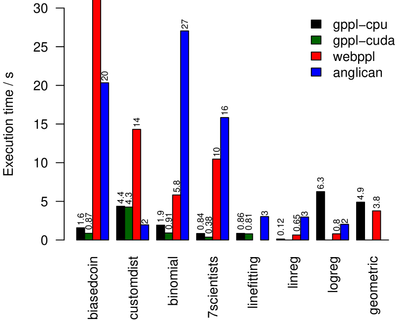
Figure 7. Execution time across all benchmarks and languages. Error bars show one standard deviation for 10 repeated measurements. Where data is omitted, the benchmark is either not supported by that language or takes more than 10 minutes to run.

The scalability for two of the benchmarks is shown in Figure 8. linefitting is the more complex of the importance sampling benchmarks, and linear_regression uses Lightweight MH inference. These results show that each language scales similarly, however the slope for CuPPL is reduced.

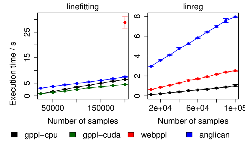
Figure 8. Performance two benchmarks using different inference methods. Error bars show one standard deviation for 10 repeated measurements.

5.2. Micro-benchmarks

Figure 9 compares the scalability of CuPPL, webppl, Anglican and Racket for two microbenchmarks. fibonacci implements the naive recursive fibonacci algorithm to test function call performance. vectorsum sums a vector of $n$ ones, to test memory bound performance.

The results show that CuPPL, Anglican and Racket all perform similarly for function call performance, whereas webppl performance is initially similar but does not scale well. For memory bound performance, webppl performs poorly. The other languages all scale similarly, however CuPPL is significantly faster.

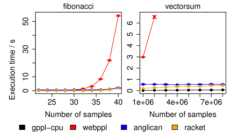
Figure 9. Performance results for two micro-benchmarks. Error bars show one standard deviation for 10 repeated measurements.

5.3. Delimited Continuation Performance

The prefix algorithm, shown in Figure 10 is used to compare our implementation against Racket (Flatt and PLT, 2010). The results are shown in Figure 11, and show that the performance of our implementation is competitive.

⬇

type List : (+ (Cons : (int, List))

(Nil : unit));

visit <- function (lst) {

case (lst) {

Nil = shift(k, Nil())

Cons (a, rst) =

(Cons(a,

shift(k,

append(k(Nil()),

reset(k(visit(rst)))))))

}

};

prefix <- function(lst) {

reset(visit(lst))

}

Figure 10. Code for the prefix benchmark in CuPPL. append is omitted for brevity. For input [1, 2, 3], this outputs [1, 1, 2, 1, 2, 3].

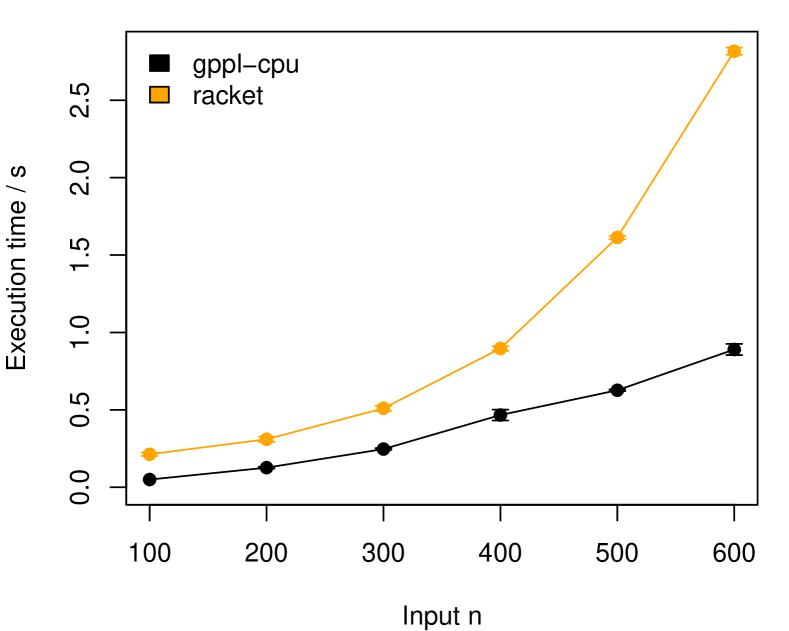
Figure 11. Execution time against input size for the prefix benchmark, comparing CuPPL to Racket.

6. Conclusions and Future Work

In this paper, we have presented CuPPL, a probabilistic programming language that generates highly efficient code for both CPUs and CUDA GPUs. The language is functional in style, and the toolchain is built on top of LLVM. Our implementation uses delimited continuations on CPU to perform inference, and custom CUDA codes on GPU.

Compared to other state of the art PPLs Anglican (Tolpin et al., 2016) and webppl (Goodman and Stuhlmüller, 2014), CuPPL achieves significantly better performance across a range of benchmarks, and scales linearly to large numbers of samples. Our implementation of delimited continuations is also competitive with Racket (Flatt and PLT, 2010).

In future, we plan to extend our language to support a greater variety of inference methods on both CPU and GPU. We are investigating parallelizable particle-based inference methods (Paige et al., 2014) for use on GPU.

References

- (1)
- clo (2018) 2018. Clojure. https://clojure.org. (2018). Accessed: 2018-02-23.
- nod (2018) 2018. NodeJS. https://nodejs.org. (2018). Accessed: 2018-02-23.
- Abadi et al. (2015) Martín Abadi, Ashish Agarwal, Paul Barham, Eugene Brevdo, Zhifeng Chen, Craig Citro, Greg S. Corrado, Andy Davis, Jeffrey Dean, Matthieu Devin, Sanjay Ghemawat, Ian Goodfellow, Andrew Harp, Geoffrey Irving, Michael Isard, Yangqing Jia, Rafal Jozefowicz, Lukasz Kaiser, Manjunath Kudlur, Josh Levenberg, Dan Mané, Rajat Monga, Sherry Moore, Derek Murray, Chris Olah, Mike Schuster, Jonathon Shlens, Benoit Steiner, Ilya Sutskever, Kunal Talwar, Paul Tucker, Vincent Vanhoucke, Vijay Vasudevan, Fernanda Viégas, Oriol Vinyals, Pete Warden, Martin Wattenberg, Martin Wicke, Yuan Yu, and Xiaoqiang Zheng. 2015. TensorFlow: Large-Scale Machine Learning on Heterogeneous Systems. (2015). https://www.tensorflow.org/ Software available from tensorflow.org.
- Asai and Kameyama (2007) Kenichi Asai and Yukiyoshi Kameyama. 2007. Polymorphic Delimited Continuations. In Proceedings of the 5th Asian Conference on Programming Languages and Systems (APLAS’07). Springer-Verlag, Berlin, Heidelberg, 239–254.
- Boehm and Weiser (1988) Hans-Juergen Boehm and Mark Weiser. 1988. Garbage Collection in an Uncooperative Environment. Software Practices and Experience 18, 9 (Sept. 1988), 807–820.
- Borgström et al. (2016) Johannes Borgström, Ugo Dal Lago, Andrew D. Gordon, and Marcin Szymczak. 2016. A Lambda-calculus Foundation for Universal Probabilistic Programming. In Proceedings of the 21st ACM SIGPLAN International Conference on Functional Programming (ICFP 2016). ACM, New York, NY, USA, 33–46.
- Carpenter et al. (2017) Bob Carpenter, Andrew Gelman, Matthew Hoffman, Daniel Lee, Ben Goodrich, Michael Betancourt, Marcus Brubaker, Jiqiang Guo, Peter Li, and Allen Riddell. 2017. Stan: A Probabilistic Programming Language. Journal of Statistical Software, Articles 76, 1 (2017), 1–32.
- Felleisen (1988) Mattias Felleisen. 1988. The Theory and Practice of First-class Prompts. In Proceedings of the 15th ACM SIGPLAN-SIGACT Symposium on Principles of Programming Languages (POPL ’88). ACM, New York, NY, USA, 180–190.
- Flatt and PLT (2010) Matthew Flatt and PLT. 2010. Reference: Racket. Technical Report PLT-TR-2010-1. PLT Design Inc. https://racket-lang.org/tr1/.
- Gaunt et al. (2016) Alexander L. Gaunt, Marc Brockschmidt, Rishabh Singh, Nate Kushman, Pushmeet Kohli, Jonathan Taylor, and Daniel Tarlow. 2016. TerpreT: A Probabilistic Programming Language for Program Induction. CoRR abs/1608.04428 (2016).
- Goodman (2013) Noah D. Goodman. 2013. The Principles and Practice of Probabilistic Programming. In Proceedings of the 40th Annual ACM SIGPLAN-SIGACT Symposium on Principles of Programming Languages (POPL ’13). ACM, New York, NY, USA, 399–402.
- Goodman et al. (2012) Noah D. Goodman, Vikash K. Mansinghka, Daniel M. Roy, Keith Bonawitz, and Joshua B. Tenenbaum. 2012. Church: a language for generative models. CoRR abs/1206.3255 (2012).
- Goodman and Stuhlmüller (2014) Noah D Goodman and Andreas Stuhlmüller. 2014. The Design and Implementation of Probabilistic Programming Languages. http://dippl.org. (2014). Accessed: 2018-02-23.
- Kiselyov and Shan (2009) Oleg Kiselyov and Chung-Chieh Shan. 2009. Embedded Probabilistic Programming. In Proceedings of the IFIP TC 2 Working Conference on Domain-Specific Languages (DSL ’09). Springer-Verlag, Berlin, Heidelberg, 360–384.
- Lattner and Adve (2004) Chris Lattner and Vikram Adve. 2004. LLVM: A Compilation Framework for Lifelong Program Analysis and Transformation. In COde Generation and Optimization. San Jose, CA, USA, 75–88.
- Lunn et al. (2009) David Lunn, David Spiegelhalter, Andrew Thomas, and Nicky Best. 2009. The BUGS project: Evolution, critique and future directions. Statistics in Medicine 28, 25 (2009), 3049–3067.
- Paige et al. (2014) Brooks Paige, Frank Wood, Arnaud Doucet, and Yee Whye Teh. 2014. Asynchronous Anytime Sequential Monte Carlo. In Advances in Neural Information Processing Systems 27, Z. Ghahramani, M. Welling, C. Cortes, N.D. Lawrence, and K.Q. Weinberger (Eds.). Curran Associates, Inc., 3410–3418.
- Ripley (2008) Brian D Ripley. 2008. Stochastic Simulation.
- Tolpin et al. (2016) David Tolpin, Jan Willem van de Meent, Hongseok Yang, and Frank Wood. 2016. Design and Implementation of Probabilistic Programming Language Anglican. arXiv preprint arXiv:1608.05263 (2016).
- Tran et al. (2017) Dustin Tran, Matthew D. Hoffman, Rif A. Saurous, Eugene Brevdo, Kevin Murphy, and David M. Blei. 2017. Deep probabilistic programming. In International Conference on Learning Representations.
- Tran et al. (2016) Dustin Tran, Alp Kucukelbir, Adji B. Dieng, Maja Rudolph, Dawen Liang, and David M. Blei. 2016. Edward: A library for probabilistic modeling, inference, and criticism. arXiv preprint arXiv:1610.09787 (2016).
- Wingate et al. (2011) David Wingate, Andreas Stuhlmueller, and Noah Goodman. 2011. Lightweight Implementations of Probabilistic Programming Languages via Transformational Compilation. In Proceedings of the Fourteenth International Conference on Artificial Intelligence and Statistics (Proceedings of Machine Learning Research), Vol. 15. PMLR, Fort Lauderdale, FL, USA, 770–778.