Unbiased Gradient Estimation for Variational Auto-Encoders
using Coupled Markov Chains

Abstract

The variational auto-encoder (VAE) is a deep latent variable model that has two neural networks in an autoencoder-like architecture; one of them parameterizes the model’s likelihood. Fitting its parameters via maximum likelihood (ML) is challenging since the computation of the marginal likelihood involves an intractable integral over the latent space; thus the VAE is trained instead by maximizing a variational lower bound. Here, we develop a ML training scheme for VAEs by introducing unbiased estimators of the log-likelihood gradient. We obtain the estimators by augmenting the latent space with a set of importance samples, similarly to the importance weighted auto-encoder (IWAE), and then constructing a Markov chain Monte Carlo coupling procedure on this augmented space. We provide the conditions under which the estimators can be computed in finite time and with finite variance. We show experimentally that VAEs fitted with unbiased estimators exhibit better predictive performance.

1 INTRODUCTION

The variational auto-encoder (VAE) [Kingma and Welling, 2014] is a deep latent variable model that uses a joint distribution $p_{\theta}(x,z)$, parameterized by $\theta$, over an observation $x$ and the corresponding latent variable $z$. The marginal log-likelihood involves an integral over the latent space,

$$\mathcal{L}(\theta):=\log p_{\theta}(x)=\log\left(\int p_{\theta}(x,z)\textrm{d}z\right).$$ (1)

As for any other latent variable model, fitting the VAE requires finding the parameters $\theta$ that best describe the observations. One (intractable) way to find $\theta$ would be via maximum likelihood, for which the gradient of Eq. 1 is required. Using Fisher’s identity, this gradient can be written as an expectation w.r.t. the posterior $p_{\theta}(z\,|\,x)$,

$$\nabla_{\theta}\mathcal{L}(\theta)=\mathbb{E}_{p_{\theta}(z\,|\,x)}\left[\nabla_{\theta}\log p_{\theta}(x,z)\right].$$ (2)

The gradient in Eq. 2 could be approximated unbiasedly if we had access to samples from $p_{\theta}(z\,|\,x)$; however, the posterior is intractable. Although we could use Markov chain Monte Carlo (MCMC) to sample approximately from it [Hoffman, 2017, Naesseth et al., 2020], this would provide a biased estimate, and the bias is difficult to quantify.

Instead, VAEs introduce an encoder $q_{\phi}(z\,|\,x)$ and learn the parameters $\theta$ by maximizing a variational evidence lower bound (ELBO) [Wainwright and Jordan, 2008, Blei et al., 2017], for which unbiased gradients are readily available [Kingma and Welling, 2014]. Burda et al. [2016] form such a bound using a set of importance samples using the encoder as proposal distribution, leading to the so-called importance weighted auto-encoder (IWAE). The standard ELBO in variational inference can be thought of as a particular instance of the IWAE bound with one importance sample, where the importance distribution is given by the encoder. However, it remains difficult to quantify the difference between the true log-likelihood and the corresponding bound.

We develop here unbiased gradient estimators of the log-likelihood for VAEs by exploiting the coupling estimators developed by Jacob et al. [2020b]. Coupling estimators allow us to obtain unbiased estimators of expectations w.r.t. an intractable target distribution by running two coupled MCMC chains for a finite number of iterations. This approach does not require that the MCMC chains converge to the target, so the unbiased estimator can be computed in a finite (but random) time. However, MCMC couplings are a generic methodology that is not readily applicable to VAEs, since it requires an MCMC kernel that mixes well and provides a suitable coupling mechanism, while at the same time yielding a low-variance estimator.

We address these issues by building coupling estimators based on the iterated sampling importance resampling (ISIR) algorithm [Andrieu et al., 2010]. ISIR is in turn based on importance sampling, and thus it uses multiple samples to reduce the variance of the estimator, similarly to the IWAE. Like the IWAE, we simultaneously fit an encoder as the proposal distribution for the importance sampling algorithm. Unfortunately, the variance of ISIR is still not small enough for fitting VAEs. To that end, we develop an extension of ISIR, called dependent iterated sampling importance resampling (DISIR), that combines the use of dependent importance samples and reparameterization ideas. DISIR drastically reduces the running time and the variance of the resulting coupling estimator. We develop a DISIR-based coupling estimator to estimate the gradient of the VAE log-likelihood.

Contributions.  Our contributions are as follows.

• We show that the unbiased gradient estimators based on ISIR are not practical for VAEs, since they require to run the Markov chains for a long time even for only moderately high-dimensional models.

• We develop DISIR, an extension of ISIR that reduces the running time and the variance of the estimators.

• We use DISIR to form unbiased gradient estimators for VAEs. The resulting estimator is widely applicable as it can be used wherever the IWAE bound is applicable.

• We prove that the unbiased gradient estimates have finite variance and can be computed in finite expected time under some regularity conditions.

• We demonstrate experimentally that VAEs fitted with the DISIR-based gradient estimators exhibit better predictive log-likelihood on binarized MNIST, fashion-MNIST, and CIFAR-10, when compared to IWAE.

2 BACKGROUND

Here, we review the IWAE bound [Burda et al., 2016] and show that it can be seen as a standard ELBO on an augmented model. Consider a model $p_{\theta}(x,z)$ of data $x$ and latent variables $z\in\mathcal{Z}$, and a proposal distribution $q_{\phi}(z\,|\,x)$, where $\theta$ and $\phi$ denote the model and proposal parameters, respectively. Let the proposal satisfy the assumption below.

Assumption 1 (The proposal and posterior have the same support).

For any $z\in\mathcal{Z}$, we have $q_{\phi}(z\,|\,x)>0$ if and only if $p_{\theta}(x,z)>0$, so that $0<w_{\theta,\phi}(z)<\infty$, where the importance weights are

$$w_{\theta,\phi}(z):=\frac{p_{\theta}(x,z)}{q_{\phi}(z\,|\,x)}.$$ (3)

The IWAE bound.  The IWAE is a lower bound of the marginal log-likelihood in Eq. 1 formed with $K\geq 1$ importance samples $z_{1:K}$ from the proposal, i.e., $\mathcal{L}(\theta)\geq\mathcal{L}_{\text{IWAE}}(\theta,\phi)$, with

$$\mathcal{L}_{\text{IWAE}}(\theta,\phi)=\mathbb{E}_{q_{\phi}(z_{1:K}\,|\,x)}\!\!\left[\log\!\left(\!\frac{1}{K}\sum_{k=1}^{K}w_{\theta,\phi}(z_{k})\!\right)\!\right]\!,$$ (4)

where $q_{\phi}(z_{1:K}\,|\,x):=\prod_{k=1}^{K}q_{\phi}(z_{k}\,|\,x)$. Eq. 4 monotonically increases with $K$, converging towards $\mathcal{L}(\theta)$ as $K\rightarrow\infty$. For the case $K=1$, it recovers the standard ELBO,

$$\mathcal{L}_{\text{ELBO}}(\theta,\phi)=\mathbb{E}_{q_{\phi}(z\,|\,x)}\left[\log w_{\theta,\phi}(z)\right].$$ (5)

The importance samples $z_{1:K}$ also provide an approximation of the posterior $p_{\theta}(z\,|\,x)$. Specifically, if we define the importance weights $w_{\theta,\phi}^{(k)}:=w_{\theta,\phi}(z_{k})$ and the normalized importance weights $\widetilde{w}_{\theta,\phi}^{(k)}\propto w_{\theta,\phi}^{(k)}$, with $\sum_{k=1}^{K}\widetilde{w}_{\theta,\phi}^{(k)}=1$, then the approximation is

$$\hat{p}_{\theta}(z\,|\,x)=\sum_{k=1}^{K}\widetilde{w}_{\theta,\phi}^{(k)}\delta_{z_{k}}(z),$$ (6)

where $\delta_{z_{k}}(\cdot)$ is the delta Dirac measure located at $z_{k}$.

Fitting VAEs.  VAEs parameterize the likelihood $p_{\theta}(x\,|\,z)$ using a distribution whose parameters are given by a neural network (decoder) that inputs the latent variable $z$. The distribution $q_{\phi}(z\,|\,x)$ is amortized [Gershman and Goodman, 2014], i.e., its parameters are computed by a neural network (encoder) that inputs the observation $x$. Fitting a VAE involves maximizing the bound (either Eq. 4 or Eq. 5) w.r.t. both $\theta$ and $\phi$ using stochastic optimization. For that, the VAE uses unbiased gradient estimators of the objective. To form such gradients, we typically assume that $q_{\phi}(z\,|\,x)$ is reparameterizable [Kingma and Welling, 2014, Rezende et al., 2014, Titsias and Lázaro-Gredilla, 2014]. For convenience, we additionally assume that we can reparameterize in terms of a Gaussian (but we can easily relax this latter assumption).

Assumption 2 (The variational distribution is reparameterizable in terms of a Gaussian).

There exists a mapping $g_{\phi}(\xi,x)$ such that by sampling $\xi\sim q(\xi)$, where $q(\xi)=\mathcal{N}(\xi;0,I)$, and setting $z=g_{\phi}(\xi,x)$, we obtain $z\sim q_{\phi}(z\,|\,x)$.

The IWAE bound as a standard ELBO.  The IWAE bound in Eq. 4 can be interpreted as a regular ELBO on an augmented latent space [Cremer et al., 2017, Domke and Sheldon, 2018], and we use this perspective in Sections 3 and 4. Indeed, consider the $K$ importance samples $z_{1:K}$ and an indicator variable $\ell\in\{1,\ldots,K\}$. We next define a generative model with latent variables $(z_{1:K},\ell)$, as well as a variational distribution, such that its ELBO recovers Eq. 4.

The augmented generative model posits that the indicator $\ell\sim\textrm{Cat}(\frac{1}{K},\ldots,\frac{1}{K})$, where Cat denotes the categorical distribution. Given $\ell$, each $z_{k}$ is distributed according to $q_{\phi}(z\,|\,x)$, except the $\ell$-th one, which follows the prior:

$$p_{\theta,\phi}(x,z_{1:K},\ell)=\frac{1}{K}\;p_{\theta}(x,z_{\ell})\prod_{k=1,k\neq\ell}^{K}q_{\phi}(z_{k}\,|\,x).$$ (7)

Under the corresponding augmented posterior distribution, $p_{\theta,\phi}(z_{1:K},\ell\,|\,x)\propto p_{\theta,\phi}(x,z_{1:K},\ell)$, the random variable $z_{\ell}$ follows the posterior $p_{\theta}(z\,|\,x)$. We next define a variational distribution on the same augmented space,

$$q_{\theta,\phi}(z_{1:K},\ell\,|\,x)=\text{Cat}\!\left(\!\ell\,|\,\widetilde{w}_{\theta,\phi}^{(1)},\cdots,\widetilde{w}_{\theta,\phi}^{(K)}\!\right)\!\prod_{k=1}^{K}q_{\phi}(z_{k}\,|\,x).$$ (8)

We recover the IWAE bound (Eq. 4) as the ELBO of the augmented model, i.e., as $\mathbb{E}_{q_{\theta,\phi}(z_{1:K},\ell\,|\,x)}\left[\log p_{\theta,\phi}(x,z_{1:K},\ell)\right]$.

Towards unbiased gradient estimation.  The gradient w.r.t. $\theta$ of the IWAE bound in Eq. 4 can be interpreted as a (biased) approximation of $\nabla_{\theta}\mathcal{L}$ from Eq. 2. To see this, note that $\nabla_{\theta}\mathcal{L}_{\text{IWAE}}=\mathbb{E}_{\hat{p}_{\theta}(z\,|\,x)}\left[\nabla_{\theta}\log p_{\theta}(x,z)\right]$; i.e., $\nabla_{\theta}\mathcal{L}_{\text{IWAE}}$ can be seen as an approximation of $\nabla_{\theta}\mathcal{L}$ where we replace the posterior $p_{\theta}(z\,|\,x)$ with the approximation $\hat{p}_{\theta}(z\,|\,x)$ in Eq. 6.

To obtain an unbiased estimate, we need an alternative approximation $\hat{p}_{\theta}(z\,|\,x)$ of $p_{\theta}(z\,|\,x)$ satisfying $\mathbb{E}_{\hat{p}_{\theta}(z\,|\,x)}\left[\nabla_{\theta}\log p_{\theta}(x,z)\right]=\nabla_{\theta}\mathcal{L}$. One such example is the empirical measure of exact samples from $p_{\theta}(z\,|\,x)$. However, as mentioned earlier, it is typically impossible to obtain such samples, as a finite run with an MCMC kernel only provides biased estimates when the chain is initialized out of equilibrium. We can obtain an approximation $\hat{p}_{\theta}(z\,|\,x)$ that leads to unbiased estimation using two coupled MCMC chains [Jacob et al., 2020b]. In Sections 3 and 4 we build on this idea to develop a method for unbiased gradient estimation.

3 IMPORTANCE SAMPLING-BASED MCMC SCHEMES

3.1 Iterated Sampling Importance Resampling (ISIR)

Here we review ISIR [Andrieu et al., 2010], an MCMC scheme that samples from the augmented posterior $p_{\theta,\phi}(z_{1:K},\ell\,|\,x)$ given by Eq. 7. Alternatively, ISIR can be interpreted as an algorithm that targets the posterior $p_{\theta}(z\,|\,x)$. Indeed, if $(z_{1:K},\ell)\sim p_{\theta,\phi}(z_{1:K},\ell\,|\,x)$ is a sample from the augmented posterior, then $z_{\ell}\sim p_{\theta}(z\,|\,x)$.

The ISIR transition kernel, $\mathcal{K}_{\textrm{ISIR}}(\cdot,\cdot\,|\,z_{1:K},\ell)$, takes the current state $(z_{1:K},\ell)$ and outputs a new state by following Algorithm 1. ISIR requires a proposal distribution; we use $q_{\phi}(z\,|\,x)$. It also requires to compute the importance weights $w_{\theta,\phi}(\cdot)$ in Eq. 3. Note that ISIR has a resampling step (Algorithm 1) that is distinct from the resampling step of sequential Monte Carlo, which would involve resampling multiple times from the categorical before mutating the samples.

The kernel is invariant w.r.t. $p_{\theta,\phi}(z_{1:K},\ell\,|\,x)$, as formalized in Proposition 5 in Section C.1, if Assumption 3 below is satisfied [Andrieu et al., 2010, 2018]. Assumption 3 holds when the proposal is at least as heavy-tailed as the target.

Assumption 3 (The importance weights are bounded).

There exists $w_{\theta,\phi}^{\textrm{max}}<\infty$ such that $w_{\theta,\phi}(z)\leq w_{\theta,\phi}^{\textrm{max}}$ $\forall z\in\mathcal{Z}$.

3.2 Dependent Iterated Sampling Importance Resampling (DISIR)

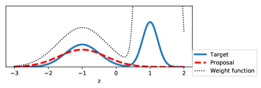
(a) Target density, proposal, and weight function.

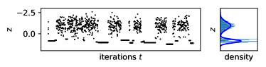
(b) A realization from the ISIR kernel.

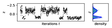
(c) A realization from the DISIR kernel.

Figure 1: Qualitative comparison of ISIR and DISIR targetting a simple target distribution (a), and the realized chains by sampling from ISIR (b) and DISIR (c) transition kernels. Due to the poor proposal choice, the weight function significantly varies across the space $z$. ISIR has a low acceptance probability, especially in high-weight states. In contrast, DISIR is able to propose and accept local moves around high-weight regions and explores the target better.

Input: Current state of the chain, $(z_{1:K},\ell)$

Output: Next state of the chain

1 Sample $\ell_{\textrm{aux}}\sim\textrm{Cat}(\frac{1}{K},\ldots,\frac{1}{K})$

2 Set $z^{\star}_{\ell_{\textrm{aux}}}=z_{\ell}$

3 Sample $z_{k}^{\star}\sim q_{\phi}(z\,|\,x)$ for $k\in\{1,\ldots,K\}\backslash\{\ell_{\textrm{aux}}\}$

4 Sample $\ell^{\star}\sim\textrm{Cat}(p_{1},\ldots,p_{K})$ with $p_{k}\propto w_{\theta,\phi}(z_{k}^{\star})$

5 Return $(z_{1:K}^{\star},\ell^{\star})$

Algorithm 1 ISIR kernel, $\mathcal{K}_{\textrm{ISIR}}(\cdot,\cdot\,|\,z_{1:K},\ell)$

For moderately high-dimensional $z$, ISIR can be inefficient. Indeed, if the importance weights become dominated by the weight of a single sample, then the corresponding Markov chain will typically get “stuck” for a large number of iterations. We illustrate this in Figure 1, which shows a one-dimensional illustrative comparison. In this toy experiment, we can observe that the ISIR chains gets stuck when the state $z^{(t)}$ corresponds to a high-weight region.

To mitigate this problem, here we develop DISIR, an extension of ISIR that uses dependent importance samples. Intuitively, this scheme proposes dependent samples $z_{1:\ell_{\textrm{aux}}-1}^{\star},z_{\ell_{\textrm{aux}}+1:K}^{\star}$ that are close to the current sample $z_{\ell_{\textrm{aux}}}^{\star}=z_{\ell}$ with high probability, in the spirit of Shestopaloff and Neal [2018]. This modification increases the probability that the chain transitions to one of the new proposed values. As a result, in practice, the gradient estimators based on DISIR have smaller variance than the ones based on ISIR.

To make samples dependent, we use the reparameterization property (see Assumption 2) and introduce dependencies among the auxiliary variables $\xi_{1:K}$; this induces dependencies among the samples in the original latent space $z_{1:K}$. That is, rather than sampling $K-1$ importance samples ($\xi^{\star}_{1:\ell_{\textrm{aux}}-1},\xi^{\star}_{\ell_{\textrm{aux}}+1:K}$) independently of $\xi^{\star}_{\ell_{\textrm{aux}}}$ (see Algorithm 1 of Algorithm 1), we use two auxiliary Markov chains, each with transition kernel $p_{\beta}(\xi^{\star}\,|\,\xi)$. Specifically, given $\xi^{\star}_{\ell_{\textrm{aux}}}$, we sample $\xi_{k}^{\star}\sim p_{\beta}(\cdot\,|\,\xi_{k-1}^{\star})$ for $k>\ell_{\textrm{aux}}$ and $\xi_{k}^{\star}\sim p_{\beta}(\cdot\,|\,\xi_{k+1}^{\star})$ for $k<\ell_{\textrm{aux}}$. The kernel $p_{\beta}(\xi^{\star}\,|\,\xi)$ must have invariant density $q(\xi)$, so that marginally $\xi_{k}^{\star}\sim q(\xi)$ for all $k$ if $\xi^{\star}_{\ell_{\textrm{aux}}}\sim q(\xi)$. This construction with two Markov chains ensures the validity of the scheme (see Section C.2 for details).

Under Assumption 2, we select a simple autoregressive normal kernel for $p_{\beta}(\xi^{\star}\,|\,\xi)$, i.e., we set

$$p_{\beta}(\xi^{\star}\,|\,\xi)=\mathcal{N}(\xi^{\star};\beta\xi,(1-\beta^{2})I).$$ (9)

Equivalently, $\xi^{\star}=\beta\xi+\sqrt{1-\beta^{2}}\xi^{\textrm{new}}$, where $\xi^{\textrm{new}}\sim\mathcal{N}(\xi;0,I)$. The parameter $\beta$ controls the strength of the correlation; we discuss its effect below.

Using the kernel in Eq. 9, we develop DISIR, which is described in Algorithm 2. DISIR replaces Algorithm 1 of Algorithm 1 with an application of the auxiliary kernel $p_{\beta}(\xi^{\star}\,|\,\xi)$ (see Algorithms 2 and 2 of Algorithm 2).

We refer to the coefficient $\beta\in[0,1)$ as the correlation strength. When $\beta=0$, we have $\xi_{k}^{\star}=\xi_{k}^{\textrm{new}}\overset{\textrm{iid}}{\sim}q(\xi)$ and this approach is simply a reparameterized version of ISIR, which favours exploration of new regions of the space. When $\beta$ approaches $1$, all the proposed values $\xi_{k}^{\star}$ become closer to the current state $\xi_{\ell}$ (which may correspond to the sample whose importance weight currently dominates). This dependency among the samples $\xi_{1:K}^{\star}$ induces dependencies among $z_{1:K}^{\star}$, resulting in more uniform importance weights. Thus, we say that this approach favours exploitation.

As given in Algorithm 2, DISIR is an MCMC scheme that targets the augmented density provided below.

Proposition 1 (Invariant distribution of DISIR).

Let Assumptions 1 and 2 hold. For any $K\geq 2$ and any $\beta\in[0,1)$, the DISIR transition kernel $\mathcal{K}_{\textrm{DISIR}}$ admits

$$p_{\theta,\phi}^{\text{\emph{DISIR}}}(\xi_{1:K},\ell\,|\,x) =\frac{1}{K}\frac{w_{\theta,\phi}(g_{\phi}(\xi_{\ell},x))q(\xi_{\ell})}{p_{\theta}(x)}$$ (10)

$$\times\prod_{k=1}^{\ell-1}p_{\beta}(\xi_{k}\,|\,\xi_{k+1})\prod_{k=\ell+1}^{K}p_{\beta}(\xi_{k}\,|\,\xi_{k-1})$$

as invariant distribution and is ergodic.

The proofs of all propositions and lemmas are provided in Appendix C.

Input: Current state of the chain $(\xi_{1:K},\ell)$ and correlation strength $\beta$

Output: New state of the chain

1 Sample $\ell_{\textrm{aux}}\sim\textrm{Cat}(\frac{1}{K},\ldots,\frac{1}{K})$

2

3Set $\xi_{\ell_{\textrm{aux}}}^{\star}=\xi_{\ell}$

4

5Sample $\xi_{k}^{\textrm{new}}\sim q(\xi)$ for $k\in\{1,\ldots,K\}\backslash\{\ell_{\textrm{aux}}\}$

6

7Set $\xi_{k}^{\star}=\beta\xi_{k-1}^{\star}+\sqrt{1-\beta^{2}}\xi_{k}^{\textrm{new}}$ for $k=\ell_{\textrm{aux}}+1,\ldots,K$

8

9Set $\xi_{k}^{\star}=\beta\xi_{k+1}^{\star}+\sqrt{1-\beta^{2}}\xi_{k}^{\textrm{new}}$ for $k=\ell_{\textrm{aux}}-1,\ldots,1$

10

11Set $z_{k}^{\star}=g_{\phi}(\xi_{k}^{\star},x)$ for $k=1,\ldots,K$

12

13Sample $\ell^{\star}\sim\textrm{Cat}(p_{1},\ldots,p_{K})$ with $p_{k}\propto w_{\theta,\phi}(z_{k}^{\star})$

14

15Return $(\xi_{1:K}^{\star},\ell^{\star})$

Algorithm 2 DISIR kernel, $\mathcal{K}_{\textrm{DISIR}}(\cdot,\cdot\,|\,\xi_{1:K},\ell)$

This target distribution has two desired properties. First, when the correlation strength $\beta\in[0,1)$, the $\ell$-th sample $z_{\ell}$ is distributed according to the posterior $p_{\theta}(z\,|\,x)$. That is, DISIR defines a Markov chain that targets Eq. 10, and $(z^{(t)}_{\ell^{(t)}})_{t\geq 0}$ is a Markov chain that converges to $p_{\theta}(z\,|\,x)$. Second, when $\beta=0$, DISIR becomes identical to a reparameterized version of ISIR. That is, it simulates a Markov chain $(\xi_{1:K}^{(t)},\ell^{(t)})_{t\geq 0}$ such that, setting each $z_{k}^{(t)}=g_{\phi}(\xi_{k}^{(t)},x)$, the Markov chain $(z_{1:K}^{(t)},\ell^{(t)})_{t\geq 0}$ obeys a law that is identical to the one simulated by ISIR. This is formalized below.

Lemma 1 (Distribution of DISIR samples).

Let Assumptions 1 and 2 hold. For any $\beta\in[0,1)$, we have $z_{\ell}=g_{\phi}(\xi_{\ell},x)\sim p_{\theta}(z\,|\,x)$ under $p_{\theta,\phi}^{\text{\emph{DISIR}}}(\xi_{1:K},\ell\,|\,x)$. Moreover, for $\beta=0$, if $(\xi_{1:K},\ell)\sim p_{\theta,\phi}^{\text{\emph{DISIR}}}(\xi_{1:K},\ell\,|\,x)$, then we have $(z_{1:K},\ell)\sim p_{\theta,\phi}(z_{1:K},\ell\,|\,x)$, where each $z_{k}=g_{\phi}(\xi_{k},x)$.

In practice, we interleave DISIR steps for which $\beta>0$ with steps for which $\beta=0$. Specifically, we define a composed kernel that consists of the consecutive application of two steps of Algorithm 2. The first step has $\beta=0$ and favours exploration; the second step has $\beta>0$ and favours exploitation. It is possible to interleave the two kernels since both can be reinterpreted as MCMC kernels targeting $p_{\theta}(z\,|\,x)$. We denote the composed kernel as $\mathcal{K}_{\textrm{ISIR-DISIR}}$.

Choice of the correlation strength.  For the second step of the composed kernel, we wish to use a value $\beta$ close to $1$ to achieve exploitation, but not too close because then we will effectively have one importance sample repeated $K$ times. We set $\beta$ following a heuristic that is based on the effective sample size (ESS), defined as $\textrm{ESS}=(\sum_{k=1}^{K}(\widetilde{w}_{\theta,\phi}^{(k)})^{2})^{-1}$. As $\beta$ becomes closer to $1$, the ESS becomes closer to $K$. We set the target ESS to $0.3K$, and we update $\beta$ after each step of the kernel, so that the ESS becomes closer to the target value. In particular, we apply the update rule $\beta\leftarrow\beta-0.01(\textrm{ESS}-0.3K)$. We also constrain the resulting $\beta\in[10^{-6},1-10^{-6}]$ to avoid numerical issues.

Since we only modify $\beta$ between iterations of the algorithm (and not while running the algorithm), the invariance of the Markov kernel w.r.t. to the target still holds. This also implies that the estimators that we derive in Section 4 are unbiased despite the adaptation of $\beta$.

3.3 DISIR Estimates of Expectations

The DISIR samples $(z^{(t)}_{\ell^{(t)}})_{t\geq 0}$ are distributed asymptotically as $p_{\theta}(z\,|\,x)$ and, in the limit of infinite samples, we can estimate expectations under $p_{\theta}(z\,|\,x)$, as $\tfrac{1}{T+1}\sum_{t=0}^{T}h(z^{(t)}_{\ell^{(t)}})\rightarrow\mathbb{E}_{p_{\theta}(z\,|\,x)}[h(z)]$ almost surely.

However, it may seem wasteful to generate $K-1$ proposals at each iteration of Algorithm 2 and then use only the $\ell$-th importance sample to estimate an expectation. The proposition below shows that it is possible to use all the $K$ importance samples: we can estimate an expectation $\mathbb{E}_{p_{\theta}(z\,|\,x)}[h(z)]$ with a weighted average of the importance samples.

Proposition 2 (The $K$ importance samples can be used for estimating expectations).

For any function $h:\mathcal{Z}\rightarrow\mathbb{R}$ such that $\mathbb{E}_{p_{\theta}(z\,|\,x)}[|h(z)|]<\infty$, we have the identity

$$\mathbb{E}_{p_{\theta}(z\,|\,x)}[h(z)]=\mathbb{E}_{p^{\text{\emph{DISIR}}}_{\theta,\phi}(\xi_{1:K},\ell\,|\,x)}\!\!\left[\sum_{k=1}^{K}\widetilde{w}_{\theta,\phi}^{(k)}h(z_{k})\right]\!,$$ (11)

where $z_{k}=g_{\phi}(\xi_{k},x)$ and the normalized importance weights are $\widetilde{w}_{\theta,\phi}^{(k)}\propto w_{\theta,\phi}(z_{k})$ with $\sum_{k=1}^{K}\widetilde{w}_{\theta,\phi}^{(k)}=1$. Setting $h(z)=\nabla_{\theta}\log p_{\theta}(x,z)$, and given that the DISIR kernel is ergodic, it follows from Eq. 2 that

$$\tfrac{1}{T+1}\sum_{t=0}^{T}\left[\sum_{k=1}^{K}\widetilde{w}_{\theta,\phi}^{(k,t)}\nabla_{\theta}\log p_{\theta}(x,z_{k}^{(t)})\right]\rightarrow\nabla_{\theta}\mathcal{L}$$ (12)

almost surely as $T\rightarrow\infty$ for any $K\geq 2$, where $z_{k}^{(t)}=g_{\phi}(\xi^{(t)}_{k},x)$ and $\widetilde{w}_{\theta,\phi}^{(k,t)}\propto w_{\theta,\phi}(z_{k}^{(t)})$.

3.4 Choice of the Proposal

Both ISIR and DISIR require a proposal distribution to sample the states $z_{k}^{\star}$, for which we use $q_{\phi}(z\,|\,x)$ (DISIR additionally requires the proposal to be reparameterizable). Here we discuss how to set the parameters $\phi$ of the proposal.

Like for IWAE, in our case $q_{\phi}(z\,|\,x)$ is a proposal distribution rather than a variational posterior. We fit $\phi$ via stochastic optimization of the IWAE bound in Eq. 4. To estimate the gradient w.r.t. $\phi$, we use the doubly reparameterized estimator [Tucker et al., 2019], which addresses some issues of the estimator of Burda et al. [2016] for large values of $K$ [Rainforth et al., 2019].

Alternatively, we could fit the encoder using the forward Kullback-Leibler (KL) divergence. This would imply to maximize $\mathbb{E}_{p_{\theta}(z\,|\,x)}\left[\log q_{\phi}(z\,|\,x)\right]$ w.r.t. $\phi$, for which we can apply the unbiased estimators of Section 4 to estimate the expectation w.r.t. $p_{\theta}(z\,|\,x)$. We leave this for future work.

4 UNBIASED GRADIENT ESTIMATION WITH MCMC COUPLINGS

4.1 Unbiased Estimation with Couplings

In this section, we review how to obtain an unbiased gradient estimator using two coupled Markov chains. We use the notation $u\in\mathcal{U}$ to refer to a generic random variable, keeping in mind that we will later set $u=[\xi_{1:K},\ell]$, i.e., the latent variables in the augmented space.

Consider the estimation of the expectation

$$H:=\mathbb{E}_{\pi(u)}\left[h(u)\right],$$ (13)

for some distribution $\pi(u)$ and function $h(u)$. As discussed in Section 2, a direct approximation $\hat{\pi}(u)$ of $\pi(u)$ via MCMC leads to a biased estimator.

We can obtain an unbiased estimator based on two coupled MCMC chains, each with invariant distribution $\pi(\cdot)$ [Glynn and Rhee, 2014, Jacob et al., 2020b]. The two chains have the same marginals at any time instant $t$, but they evolve according to a joint transition kernel $\mathcal{K}_{\textrm{C}}$. Let $\mathcal{K}(\cdot\,|\,u)$ be the marginal transition kernel of each chain, and let $\mathcal{K}_{\textrm{C}}(\cdot,\cdot\,|\,u,\bar{u})$ be a joint kernel that takes the state of both chains (denoted $u$ and $\bar{u}$) and produces the new state of both chains.

We next review the unbiased estimator of Vanetti and Doucet [2020] which reduces the variance of the estimator of Jacob et al. [2020b]. The main idea is to consider a lag $L\geq 1$ and jointly sample the states of both chains $(u^{(t)},\bar{u}^{(t-L)})$ conditioned on their previous states, i.e., $(u^{(t-1)},\bar{u}^{(t-L-1)})$. We then use (a finite number of) the samples from each chain to obtain the unbiased estimator (Appendix A shows how to derive it). Practically, we initialize the first Markov chain from some (arbitrary) initial distribution $\pi_{0}(\cdot)$, i.e., $u^{(0)}\sim\pi_{0}(u)$. We then sample this Markov chain using the marginal kernel $\mathcal{K}$, i.e., $u^{(t)}\sim\mathcal{K}(u\,|\,u^{(t-1)})$ for $t=1,\ldots,L$. After $L$ steps, we draw the initial state of the second Markov chain $\bar{u}^{(0)}$ (potentially conditionally upon $u^{(L-1)},u^{(L)}$), such that marginally $\bar{u}^{(0)}\sim\pi_{0}(u)$. Afterwards, for $t>L$, we draw both states jointly as $(u^{(t)},\bar{u}^{(t-L)})\sim\mathcal{K}_{\textrm{C}}(u,\bar{u}\,|\,u^{(t-1)},\bar{u}^{(t-L-1)})$.

The joint kernel $\mathcal{K}_{\textrm{C}}$ is chosen such that, after some time, both chains produce the same exact realizations of the random variables, i.e., $u^{(t)}=\bar{u}^{(t-L)}$ for $t\geq\tau$. Here, $\tau$ is the meeting time, defined as the first time instant in which both chains meet, $\tau=\inf\{t\geq L:u^{(t)}=\bar{u}^{(t-L)}\}$ (it could be infinite, but we design the joint kernel so that $\tau$ is a random variable of finite expected value).

Based on this coupling procedure, the unbiased estimator of Eq. 13 by Vanetti and Doucet [2020] is (see Appendix A)

$$\hat{H}\!=\!\frac{1}{L}\!\left(\sum_{t=t_{0}}^{t_{0}+L-1}\!\!\!\!\!h(u^{(t)})\!+\!\!\!\!\sum_{t=t_{0}+L}^{\tau-1}\!\!\!\!\left(\!h(u^{(t)})\!-\!h(\bar{u}^{(t-L)})\!\right)\!\!\right)\!\!,$$ (14)

where $t_{0}$ is a constant that plays the role of the burn-in period, although it is not a burn-in period in the usual sense, since we do not require the Markov chains to converge. Indeed, the estimator in Eq. 14 requires us to run the coupled Markov chains until they meet each other. Given that we design the joint kernel such that the meeting time $\tau$ is finite, this implies that we obtain the unbiased estimator in finite time.

We can also think of this unbiased coupling procedure as providing an empirical approximation $\hat{\pi}(\cdot)$ of $\pi(\cdot)$,

$$\hat{\pi}(u)\!=\!\frac{1}{L}\!\left(\sum_{t=t_{0}}^{t_{0}+L-1}\!\!\!\!\!\delta_{u^{(t)}}\!(u)\!+\!\!\!\!\sum_{t=t_{0}+L}^{\tau-1}\!\!\!\!\!\left(\delta_{u^{(t)}}\!(u)\!-\!\delta_{\bar{u}^{(t-L)}}(u)\right)\!\!\right)\!\!.$$ (15)

We next provide sufficient conditions that ensure that the estimator in Eq. 14 can be computed in expected finite time and has finite variance. These conditions are similar as for the original estimator of [Jacob et al., 2020b, Middleton et al., 2020] but the proof is slightly different.

Proposition 3 (The unbiased estimator can be computed in finite time and has finite variance).

Assume the following conditions hold:

1. (Convergence of the Markov chain.) Each of the two chains marginally starts from a distribution $\pi_{0}$, evolves according to a transition kernel $\mathcal{K}$ and is such that $\mathbb{E}\left[h(u^{(t)})\right]\rightarrow\mathbb{E}_{\pi(u)}\left[h(u)\right]$ as $t\rightarrow\infty$.

2. (Finite high-order moment.) There exist $\eta>0$ and $D<\infty$ such that $\mathbb{E}\left[\left|h(u^{(t)})\right|^{2+\eta}\right]\leq D$   $\forall t\geq 0$.

3. (Distribution of the meeting time.) There exists an almost surely finite meeting time $\tau=\inf\{t\geq L:u^{(t)}=\bar{u}^{(t-L)}\}$ such that $\mathbb{P}(\tau>t)\leq Ct^{-\kappa}$ for some $C<\infty$ and $\kappa>2(2\eta^{-1}+1),$ where $\eta$ appears in Condition (b).

4. (The chains stay together after meeting.) We have $u^{(t)}=\bar{u}^{(t-L)}$ for all $t\geq\tau$.

Then, Eq. 14 is an unbiased estimator of $\mathbb{E}_{\pi(u)}[h(u)]$ that can be computed in finite expected time and has finite variance.

Conditions (a) and (d) can be satisfied by careful design of the joint kernel $\mathcal{K}_{\textrm{C}}$. Condition (b) is a mild integrability condition. Condition (c) can be satisfied if the marginal kernel $\mathcal{K}$ is (only) polynomially ergodic and some additional mild irreducibility and aperiodicity conditions on the joint kernel $\mathcal{K}_{\textrm{C}}$ hold [Middleton et al., 2020].

4.2 Coupling DISIR

Here we describe the main algorithm of this paper: an estimator based on two coupled Markov chains, each evolving according to the DISIR transition kernel from Section 3.2. That is, we build a joint kernel $\mathcal{K}_{\textrm{C}}$ for unbiased gradient estimation. We denote the joint kernel as $\mathcal{K}_{\textrm{C-DISIR}}((\cdot,\cdot),(\cdot,\cdot)\,|\,(\xi_{1:K},\ell),(\bar{\xi}_{1:K},\bar{\ell}))$. It inputs the current state of both Markov chains, $(\xi_{1:K},\ell)$ and $(\bar{\xi}_{1:K},\bar{\ell})$, and returns their new states.

The coupled DISIR kernel (C-DISIR) is given in Algorithm 3. It resembles the DISIR kernel of Algorithm 2, and in fact, as required, it behaves as $\mathcal{K}_{\textrm{DISIR}}(\cdot,\cdot\,|\,\xi_{1:K},\ell)$ marginally if we ignore one of the two Markov chains. Thus, Algorithm 3 guarantees that the marginal stationary distribution of each chain is $p^{\textrm{DISIR}}_{\theta,\phi}(\xi_{1:K},\ell\,|\,x)$ (Eq. 10).

Input: Current state of both chains, $(\xi_{1:K},\ell)$ and $(\bar{\xi}_{1:K},\bar{\ell})$, and correlation strength $\beta$

Output: New state of both chains

1 Sample $\ell_{\textrm{aux}}\sim\textrm{Cat}(\frac{1}{K},\ldots,\frac{1}{K})$

2 Set $\xi_{\ell_{\textrm{aux}}}^{\star}=\xi_{\ell}$ and $\bar{\xi}_{\ell_{\textrm{aux}}}^{\star}=\bar{\xi}_{\bar{\ell}}$

3 Sample $\xi_{k}^{\textrm{new}}\sim q(\xi)$ for $k\in\{1,\ldots,K\}\backslash\{\ell_{\textrm{aux}}\}$

4 Set $\xi_{k}^{\star}=\beta\xi_{k-1}^{\star}+\sqrt{1-\beta^{2}}\xi_{k}^{\textrm{new}}$ and $\bar{\xi}_{k}^{\star}=\beta\bar{\xi}_{k-1}^{\star}+\sqrt{1-\beta^{2}}\xi_{k}^{\textrm{new}}$ for $k=\ell_{\textrm{aux}}+1,\ldots,K$

5 Set $\xi_{k}^{\star}=\beta\xi_{k+1}^{\star}+\sqrt{1-\beta^{2}}\xi_{k}^{\textrm{new}}$ and $\bar{\xi}_{k}^{\star}=\beta\bar{\xi}_{k+1}^{\star}+\sqrt{1-\beta^{2}}\xi_{k}^{\textrm{new}}$ for $k=\ell_{\textrm{aux}}-1,\ldots,1$

6 Set $z_{k}^{\star}=g_{\phi}(\xi_{k}^{\star},x)$ and $\bar{z}_{k}^{\star}=g_{\phi}(\bar{\xi}_{k}^{\star},x)$ for $k=1,\ldots,K$

7 Sample $\ell^{\star},\bar{\ell}^{\star}\sim\mathcal{K}_{\textrm{C-Cat}}(\ell,\bar{\ell}\,|\,(w_{\theta,\phi}(z_{1}^{\star}),\ldots,w_{\theta,\phi}(z_{K}^{\star})),$ $(w_{\theta,\phi}(\bar{z}_{1}^{\star}),\ldots,w_{\theta,\phi}(\bar{z}_{K}^{\star})))$ from the maximal coupling kernel (Algorithm 5 in Appendix B)

Return $((\xi_{1:K}^{\star},\ell^{\star}),(\bar{\xi}_{1:K}^{\star},\bar{\ell}^{\star}))$

Algorithm 3 C-DISIR kernel for two coupled chains, $\mathcal{K}_{\textrm{C-DISIR}}((\cdot,\cdot),(\cdot,\cdot)\,|\,(\xi_{1:K},\ell),(\bar{\xi}_{1:K},\bar{\ell}))$

The indicators $(\ell^{\star},\bar{\ell}^{\star})$ are sampled jointly from a kernel $\mathcal{K}_{\textrm{C-Cat}}$ (Algorithm 3 of Algorithm 3), which is given in Appendix B. This corresponds to the maximal coupling kernel for two categorical distributions [Lindvall, 2002].

When the correlation strength $\beta=0$, i.e., when DISIR is equivalent to ISIR, coupling may occur; that is, Algorithm 3 may return the same state for both chains. To see this, note that when $\beta=0$, Algorithm 3 shares the same values of the noise values generating the importance samples for both chains, i.e., $\xi_{k}^{\star}=\bar{\xi}^{\star}_{k}$ for $k\neq\ell_{\textrm{aux}}$, while the $\ell_{\textrm{aux}}$-th importance sample is set to the current state of each chain, i.e., $\xi_{\ell_{\textrm{aux}}}^{\star}=\xi_{\ell}$ and $\bar{\xi}_{\ell_{\textrm{aux}}}^{\star}=\bar{\xi}_{\bar{\ell}}$. Thus, if the indicators sampled in Algorithm 3 take the same value (i.e., $\ell^{\star}=\bar{\ell}^{\star}$) and this value is different from $\ell_{\textrm{aux}}$, then both chains meet. After meeting, for any future iteration of the joint kernel, the states of both chains are guaranteed to be identical to each other. On the contrary, when the correlation strength $\beta\neq 0$, coupling cannot occur. However, for any $\beta\in[0,1)$, Algorithm 3 guarantees that the chains remain equal to each other once they have previously met.

We use a composed kernel that consists of the consecutive application of two steps of Algorithm 3. The first step has $\beta=0$; in this step the chains may meet each other. The second step has $\beta>0$, which favours exploitation. As discussed in Section 3.2, it is valid to combine these two kernels. We denote this composed joint kernel as $\mathcal{K}_{\textrm{C-ISIR-DISIR}}$.

Input: The constant $t_{0}$ and the lag $L$

Output: An unbiased estimator of $\nabla_{\theta}\mathcal{L}$

1 Initialize $\xi_{k}\sim q(\xi)$ and $\bar{\xi}_{k}\sim q(\xi)$ for $k=1,\ldots,K$

2 Initialize $\ell\sim\textrm{Cat}(\frac{1}{K},\ldots,\frac{1}{K})$ and $\bar{\ell}\sim\textrm{Cat}(\frac{1}{K},\ldots,\frac{1}{K})$

3 for $t=1,\ldots,L$ do

4       Sample $(\xi_{1:K}^{(t)},\ell^{(t)})\sim\mathcal{K}_{\textrm{ISIR-DISIR}}(\cdot,\cdot\,|\,\xi_{1:K}^{(t-1)},\ell^{(t-1)})$ (two steps of Algorithm 2, with $\beta=0$ then $\beta>0$)

5      

6 end for

7Set the iteration $t=L$

8 while $t<t_{0}+L-1$ or the two chains have not met do

9       Sample $((\xi_{1:K}^{(t+1)},\ell^{(t+1)}),(\bar{\xi}_{1:K}^{(t-L+1)},\bar{\ell}^{(t-L+1)}))\sim\mathcal{K}_{\textrm{C-ISIR-DISIR}}((\cdot,\cdot),(\cdot,\cdot)\,|\,(\xi_{1:K}^{(t)},\ell^{(t)}),(\bar{\xi}_{1:K}^{(t-L)},\bar{\ell}^{(t-L)}))$ (two steps of Algorithm 3, with $\beta=0$ then $\beta>0$)

10       Increase $t\leftarrow t+1$

11      

12 end while

13Return the estimator from Eq. 14 using the function $h(\xi_{1:K},\ell):=\sum_{k=1}^{K}\widetilde{w}_{\theta,\phi}^{(k)}\nabla_{\theta}\log p_{\theta}(x,z_{k})$

Algorithm 4 Unbiased estimation with C-ISIR-DISIR

Unbiased gradient estimation with C-ISIR-DISIR.  Algorithm 4 describes the procedure that provides an unbiased estimator of $\nabla_{\theta}\mathcal{L}$. It samples two Markov chains, $(\xi_{1:K}^{(t)},\ell^{(t)})$ and $(\bar{\xi}_{1:K}^{(t)},\bar{\ell}^{(t)})$, by inducing a coupling between the state of the first chain at time $t$ and the state of the second chain at time $t-L$, where $L\geq 1$ is the lag. After both chains meet, it returns the unbiased gradient estimator using Eq. 14 for the function $h(\xi_{1:K},\ell):=\sum_{k=1}^{K}\widetilde{w}_{\theta,\phi}^{(k)}\nabla_{\theta}\log p_{\theta}(x,z_{k})$ (applying Proposition 2), where $z_{k}=g_{\phi}(\xi_{k},x)$ and the normalized importance weights are $\widetilde{w}_{\theta,\phi}^{(k)}\propto w_{\theta,\phi}(z_{k})$. Algorithm 4 provides a practical unbiased estimator, as we show next.

Proposition 4.

Let Assumptions 1, 2 and 3 hold and condition (b) of Proposition 3 be satisfied. For any $K\geq 2$, Algorithm 4 returns an unbiased estimator of $\nabla_{\theta}\mathcal{L}$ of finite variance that can be computed in finite expected time. Additionally, $\mathbb{E}[\tau]$ can be upper bounded by a quantity decreasing with $K$.

5 RELATED WORK

Our estimator builds on previous work discussed in the former sections. We now review other related works.

ISIR, as well as other particle MCMC algorithms, has been previously used for smoothing in state-space models [Andrieu et al., 2010] and for (biased) estimation of $\nabla_{\theta}\mathcal{L}$ [Naesseth et al., 2020]. Coupled variants of these algorithms have also been previously developed for unbiased smoothing [Jacob et al., 2020a, Middleton et al., 2019]. Indeed, Algorithm 3 for $\beta=0$ has been used by Jacob et al. [2020a] (without reparameterization). However, we found experimentally that the unbiased estimators based on coupled ISIR suffer from high variance for moderately high dimensions, making them impractical for VAEs. The estimators based on coupled DISIR with $\beta\approx 1$ address this issue.

An unbiased estimator based on a coupled Gibbs sampler has also been presented for restricted Boltzmann machines [Qiu et al., 2019], but this method is not applicable for VAEs. An alternative unbiased gradient estimator for VAEs, based on Russian roulette ideas, was developed by Luo et al. [2020]. However, this estimator suffers from high variance (potentially infinite), and requires additional variance reduction methods such as gradient clipping, which defeats the purpose of unbiased gradient estimation. In our experiments, we use RMSProp and no gradient clipping is needed.

Dieng and Paisley [2019] maximize the marginal log-likelihood of the data using an expectation maximization scheme that gives a consistent (but not unbiased) estimator.

Finally, note that the coupling estimators approximate the gradient w.r.t. $\theta$, and are orthogonal to the methods that improve the expressiveness of the encoder $q_{\phi}(z\,|\,x)$, such as semi-implicit methods [Yin and Zhou, 2018, Titsias and Ruiz, 2019] or normalizing flows [Rezende and Mohamed, 2015, Kingma et al., 2016, Papamakarios et al., 2017, Tomczak and Welling, 2016, 2017, Dinh et al., 2017], to name a few. These methods could be used together with the coupling estimators to obtain a more flexible proposal distribution, which could improve the mixing of the Markov chains.

6 EXPERIMENTS

In Section 6.1, we study the bias and variance of different estimators in an experiment where we have access to the exact gradient $\nabla_{\theta}\mathcal{L}$. In Section 6.2, we study the predictive performance of VAEs trained with coupled DISIR and show that models fitted with unbiased estimators outperform those fitted via ELBO or IWAE maximization. We implement all the estimators in JAX [Babuschkin et al., 2020].

6.1 Probabilistic principal component analysis

We first consider probabilistic principal component analysis (PPCA), as for this model we have access to the exact gradient $\nabla_{\theta}\mathcal{L}$. The model is $p_{\theta}(x,z)=\mathcal{N}(z;0,I)\mathcal{N}(x;\theta_{0}+\theta_{1}^{\top}z,0.1I)$, where $z\in\mathbb{R}^{100}$. We randomly set the model parameters $\theta$ and fit a variational distribution $q_{\phi}(z\,|\,x)$ by maximizing the IWAE bound w.r.t. $\phi$ with $K=100$ importance samples on binarized MNIST [Salakhutdinov and Murray, 2008]. The distribution $q_{\phi}(z\,|\,x)$ is a fully factorized Gaussian whose parameters depend linearly on $x$.

We obtain the exact gradient, $\nabla_{\theta}\mathcal{L}=\sum_{n=1}^{N}\nabla_{\theta}\log p_{\theta}(x_{n})$, for a batch of $N=100$ datapoints, and we compare it against four gradient estimators. Two estimators are the gradients of the ELBO and IWAE bounds ($\hat{\nabla}_{\theta}\mathcal{L}_{\text{ELBO}}$ and $\hat{\nabla}_{\theta}\mathcal{L}_{\text{IWAE}}$). The third one is the unbiased estimator obtained with coupled ISIR, i.e., a variant of Algorithm 4 where we replace the $\mathcal{K}_{\textrm{C-ISIR-DISIR}}$ kernel with $\mathcal{K}_{\textrm{C-ISIR}}$ (which is equivalent to $\mathcal{K}_{\textrm{C-DISIR}}$ with correlation strength $\beta=0$). The fourth estimator is based on Algorithm 4. For all the estimators, we use the same (fixed) distribution $q_{\phi}(z\,|\,x)$. For the coupling estimators, we set $t_{0}=1$ and lag $L=10$.

We obtain $50{,}000$ samples from each estimator, and compute the (signed) error $\hat{\nabla}_{\theta}\mathcal{L}-\nabla_{\theta}\mathcal{L}$ for each sample. We show in Figure 2 the boxplot representation of the error for a randomly chosen component of the gradient w.r.t. the intercept term. (In Section D.1, we show a randomly chosen weight term in Figure 5, and the average over components in Figure 6.) As expected, the estimators of the ELBO and IWAE gradients are biased. The boxplots for C-ISIR and C-ISIR-DISIR are consistent with the unbiasedness of the estimators, and the one based on C-ISIR-DISIR has smaller variance. This property is key for fitting more complex models such as VAEs.

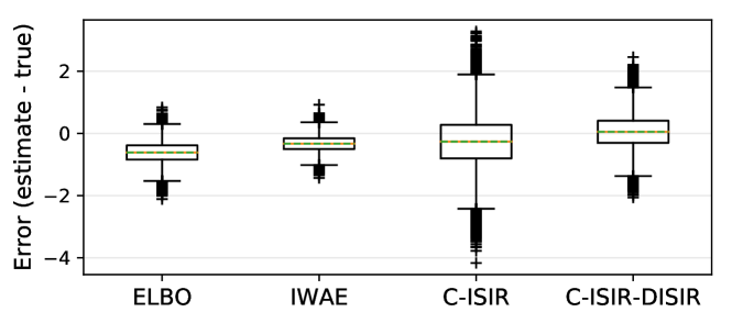
Figure 2: Boxplot representation of the error of different estimators for the gradient w.r.t. one of the intercepts of the PPCA model. The estimators based on variational bounds (ELBO and IWAE) are biased. Among the two unbiased estimators based on couplings, the one based on Algorithm 4 (C-ISIR-DISIR) exhibits lower variance.

6.2 Variational auto-encoder

Now we apply the coupling estimators to fit VAEs and compare the predictive performance to the maximization of the ELBO and IWAE objectives. (We also implemented the method of Luo et al. [2020], but we found it led to unstable optimization despite using gradient clipping.) We provide further details on the experimental setup in Section D.2.

Binarized MNIST.  We first fit a VAE on the statically binarized MNIST dataset. We use $K=10$ importance samples and explore the dimensionality $D=\{20,100,300\}$ of $z\in\mathbb{R}^{D}$. We use RMSProp [Tieleman and Hinton, 2012] in the stochastic optimization procedure. For the coupling estimators, we set $t_{0}=1$ step and the lag $L=10$.

Following Wu et al. [2017], we estimate the predictive log-likelihood using annealed importance sampling (AIS) [Neal, 2001]. Specifically, we use $16$ independent AIS chains, with $10{,}000$ intermediate annealing distributions, and a transition operator consisting of one Hamiltonian Monte Carlo (HMC) trajectory with $10$ leapfrog steps and adaptive acceptance rate tuned to $0.65$. For CIFAR-10, we use $4$ AIS chains with $7{,}500$ intermediate distributions and $5$ HMC leapfrog steps. As this procedure is computationally intensive, we only evaluate the train log-likelihood on the current data batch, but we evaluate the log-likelihood on the entire test set at the end of the optimization.

Figure 3(a) shows the evolution of the train log-likelihood; the error bars correspond to the standard deviation of $10$ independent runs. (Figure 7 in Section D.3 shows similar plots for varying $D$.) Table 2(a) shows the test log-likelihood after $300$ epochs. The VAE models fitted with the unbiased estimator of Algorithm 4 have better predictive performance.

The $\mathcal{K}_{\textrm{C-ISIR-DISIR}}$ kernel in Algorithm 4 is key for obtaining this improved performance. As a comparison, replacing it with $\mathcal{K}_{\textrm{C-ISIR}}$ leads to a test log-likelihood value of $-90.70\pm 0.08$ for $D=20$, i.e., it is worse than using the standard ELBO (and the gap with the ELBO gets larger for increasing dimensionality $D$). Moreover, $\mathcal{K}_{\textrm{C-ISIR-DISIR}}$ alleviates the computational complexity of $\mathcal{K}_{\textrm{C-ISIR}}$, as measured by the number of MCMC iterations it requires. Figure 4 compares the histograms of the meeting time $\tau$ for both kernels; C-ISIR-DISIR requires significantly fewer iterations. (Figure 8 in Section D.4 shows that the histograms behave similarly across different values of $D$.)

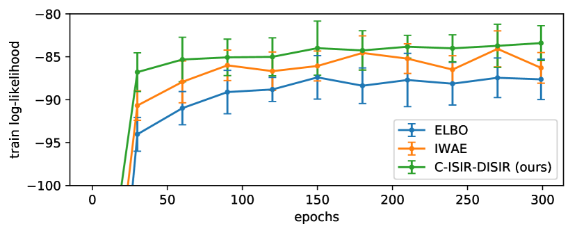
(a) Results on binarized MNIST for $D=100$. The unbiased estimator from Algorithm 4 provides better performance.

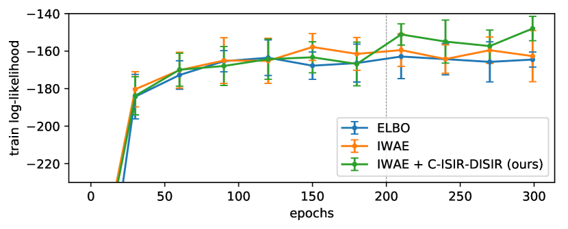
(b) Results on fashion-MNIST. After switching from the IWAE to the unbiased estimator at epoch $200$, the performance improves.

Figure 3: Train log-likelihood for a VAE.

Table 1: Test log-likelihood for the VAE. The unbiased estimators obtained via the coupled ISIR-DISIR kernel produce models with better predictive performance.

	dimensionality of $z$
	$20$	$100$	$300$
ELBO	$-90.05\pm 0.21$	$-89.96\pm 0.14$	$-90.63\pm 0.12$
IWAE	$-88.06\pm 0.08$	$-88.07\pm 0.06$	$-89.05\pm 0.08$
C-ISIR-DISIR	$\mathbf{-87.29\pm 0.08}$	$\mathbf{-86.75\pm 0.10}$	$\mathbf{-88.10\pm 0.08}$

(a) Binarized MNIST.

	Fashion-MNIST	CIFAR-10
ELBO	$-173.36\pm 0.40$	$-152.06\pm 0.30$
IWAE	$-170.50\pm 0.30$	$-149.72\pm 0.39$
IWAE + C-ISIR-DISIR	$\mathbf{-168.19\pm 0.32}$	$\mathbf{-148.40\pm 0.27}$

(b) Fashion-MNIST and CIFAR-10.

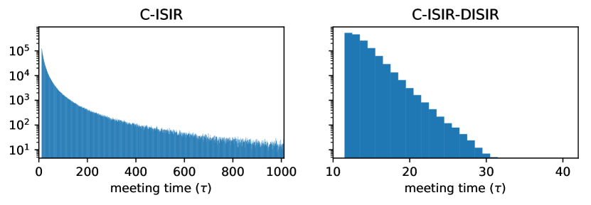
Figure 4: Histogram of the meeting time for a VAE fitted on binarized MNIST with $D=300$. The histogram corresponding to C-ISIR has significantly heavier tails, which results in higher computational complexity of the overall estimator. Moreover, C-ISIR occasionally ($1\%$) reaches the maximum allowed number of MCMC iterations (hard-coded at around $1{,}000$), which induces a small bias in the estimator. C-ISIR-DISIR does not suffer from this issue.

The improved performance over IWAE comes at the expense of computational complexity. The cost of Algorithm 4 is roughly $10$ times the cost of computing $\hat{\nabla}_{\theta}\mathcal{L}_{\text{IWAE}}$.

Fashion-MNIST and CIFAR-10.  The estimator based on Algorithm 4 leads to improved models but it is also computationally more expensive. We now study the effect of switching to Algorithm 4 after fitting a VAE using the IWAE objective. That is, we first fit the VAE using the IWAE objective for $200$ epochs, and then refine the result with the unbiased estimator based on $\mathcal{K}_{\textrm{C-ISIR-DISIR}}$. We use two datasets, fashion-MNIST [Xiao et al., 2017] and CIFAR-10 [Krizhevsky, 2009], and set $D=100$.

Figure 3(b) shows the train log-likelihood during optimization for fashion-MNIST. After switching from the IWAE objective to the unbiased estimator of Algorithm 4, it improves. Additionally, Table 2(b) shows the test log-likelihood on both fashion-MNIST and CIFAR-10 after $300$ epochs. We can conclude that switching to an unbiased gradient estimator boosts the predictive performance of the VAE.

7 DISCUSSION

We have developed a practical algorithm to obtain unbiased estimators of the gradient of the log-likelihood for intractable models, and we have shown empirically that VAEs fitted with unbiased estimators exhibit better predictive performance. Compared to ELBO or IWAE gradients, the main limitation of this approach is its higher computational cost and the fact that the running time is random. While one could obtain more accurate estimators simply by increasing the number of samples of the IWAE bound, this would significantly increase the memory requirement, making it unpractical for datasets like CIFAR-10, and it would also remain biased for any (finite) number of samples.

The topic of coupling estimators is currently an active research field. We expect future work will improve the practical applicability of such estimators using methods like, e.g., control variates [Craiu and Meng, 2020].

Appendix A DERIVATION OF THE COUPLING ESTIMATOR

Consider the expectation in Eq. 13. One choice to estimate the expectation is to build an MCMC kernel $\mathcal{K}(\cdot\,|\,u)$ that has $\pi(u)$ as its stationary distribution, run the Markov chain for some number of iterations $T$ to obtain samples $u^{(0)},u^{(1)},\ldots,u^{(T)}$, and then approximate the expectation as $\mathbb{E}_{\pi(u)}\left[h(u)\right]\approx\frac{1}{T-t_{0}+1}\sum_{t=t_{0}}^{T}h(u^{(t)})$, where the initial $t_{0}$ samples are thrown away as they are part of the burn-in period. However, this estimator is biased when the number of iterations $T$ is finite.Instead, MCMC couplings provide an unbiased estimator in finite time [Glynn and Rhee, 2014, Jacob et al., 2020b]. Coupling estimators use two MCMC chains, each with invariant distribution $\pi(\cdot)$, which evolve according to a marginal transition kernel $\mathcal{K}(\cdot\,|\,u)$ and a joint transition kernel $\mathcal{K}_{\textrm{C}}(\cdot,\cdot\,|\,u,\bar{u})$. In our paper, we rely on a slight variation over the approach of Jacob et al. [2020b] proposed by Vanetti and Doucet [2020], which provides a construction also used by Biswas et al. [2019].

Consider an integer $L\geq 1$. We draw the first Markov chain as $u^{(0)}\sim\pi_{0}(u)$ and $u^{(t)}\sim\mathcal{K}(u\,|\,u^{(t-1)})$ for $t=1,\ldots,L$. We then draw $\bar{u}^{(0)}$ (potentially conditionally upon $u^{(L-1)},u^{(L)}$) such that marginally $\bar{u}^{(0)}\sim\pi_{0}(z)$. For $t>L$, we draw both states jointly as $u^{(t)},\bar{u}^{(t-L)}\sim\mathcal{K}_{\textrm{C}}(u,\bar{u}\,|\,u^{(t-1)},\bar{u}^{(t-L-1)})$. The meeting time is defined as $\tau=\inf\{t\geq L:u^{(t)}=\bar{u}^{(t-L)}\}$.

We now provide an informal derivation of the estimator. First, we write the expectation of interest as

$$\mathbb{E}_{\pi(u)}\left[h(u)\right]=\lim_{N\rightarrow\infty}\frac{1}{L}\sum_{t=N-L+1}^{N}\mathbb{E}[h(u^{(t)})]$$

$$=\lim_{N\rightarrow\infty}\frac{1}{L}\Big{\{}\sum_{t=t_{0}}^{t_{0}+L-1}\mathbb{E}[h(u^{(t)})]+\sum_{t=t_{0}+L}^{N}\mathbb{E}[h(u^{(t)})]$$

$$-\sum_{t=t_{0}}^{N-L}\mathbb{E}[h(u^{(t)})]\Big{\}}.$$ (16)

Since $N\rightarrow\infty$, then the term within the limit can be equivalently rewritten as

$$\frac{1}{L}\sum_{t=N-L+1}^{N}\mathbb{E}[h(u^{(t)})]=\frac{1}{L}\Big{\{}\sum_{t=t_{0}}^{t_{0}+L-1}\mathbb{E}[h(u^{(t)})]$$

$$+\sum_{t=t_{0}+L}^{N}\mathbb{E}[h(u^{(t)})]-\sum_{t=t_{0}+L}^{N}\mathbb{E}[h(u^{(t-L)})]\Big{\}}.$$ (17)

Taking into account that $u^{(t)}$ and $\bar{u}^{(t)}$ have the same marginal distribution, then we can replace $u^{(t-L)}$ with $\bar{u}^{(t-L)}$,

$$\frac{1}{L}\sum_{t=N-L+1}^{N}\mathbb{E}[h(u^{(t)})]=\frac{1}{L}\Big{\{}\sum_{t=t_{0}}^{t_{0}+L-1}\mathbb{E}[h(u^{(t)})]$$

$$+\sum_{t=t_{0}+L}^{N}\mathbb{E}[h(u^{(t)})]-\sum_{t=t_{0}+L}^{N}\mathbb{E}[h(\bar{u}^{(t-L)})]\Big{\}}.$$ (18)

We now combine the two sums in the right,

$$\frac{1}{L}\sum_{t=N-L+1}^{N}\mathbb{E}[h(u^{(t)})]=\frac{1}{L}\Big{\{}\sum_{t=t_{0}}^{t_{0}+L-1}\mathbb{E}[h(u^{(t)})]$$

$$+\sum_{t=t_{0}+L}^{N}\mathbb{E}[h(u^{(t)})-h(\bar{u}^{(t-L)})]\Big{\}}.$$ (19)

We now apply the fact that the two chains meet after some time $\tau$, i.e., $u^{(t)}=\bar{u}^{(t-L)}$ for $t\geq\tau$. This gives

$$\frac{1}{L}\sum_{t=N-L+1}^{N}\mathbb{E}[h(u^{(t)})]=\frac{1}{L}\Big{\{}\sum_{t=t_{0}}^{t_{0}+L-1}\mathbb{E}[h(u^{(t)})]$$

$$+\sum_{t=t_{0}+L}^{N\wedge(\tau-1)}\mathbb{E}[h(u^{(t)})-h(\bar{u}^{(t-L)})]\Big{\}}.$$ (20)

When we consider the limit $N\rightarrow\infty$, the sum in the r.h.s. no longer depends on $N$; instead, it only contains (at most) $\tau-t_{0}-L$ terms,

$$\mathbb{E}_{\pi(u)}\left[h(u)\right]=\lim_{N\rightarrow\infty}\frac{1}{L}\sum_{t=N-L+1}^{N}\mathbb{E}[h(u^{(t)})]$$ (21)

$$=\frac{1}{L}\Big{\{}\!\!\!\sum_{t=t_{0}}^{t_{0}+L-1}\!\!\!\!\mathbb{E}[h(u^{(t)})]+\!\!\sum_{t=t_{0}+L}^{\tau-1}\!\!\!\mathbb{E}[h(u^{(t)})-h(\bar{u}^{(t-L)})]\Big{\}}.$$

From this expression, we can obtain the unbiased estimator of $\mathbb{E}_{\pi(u)}\left[h(u)\right]$ as given in Eq. 14.

Appendix B MAXIMAL COUPLING KERNEL FOR CATEGORICAL DISTRIBUTIONS

Here we describe the maximal coupling kernel for two categorical distributions [Lindvall, 2002], which is used by the coupled DISIR procedure from Section 4.2 (more specifically, in Algorithm 3 of Algorithm 3).

The kernel $\mathcal{K}_{\textrm{C-Cat}}$ is summarized in Algorithm 5. It takes two (possibly unnormalized) probability vectors, $(w_{1},\ldots,w_{K})$ and $(v_{1},\ldots,v_{K})$, and returns a realization of two coupled categorical random variables $(\ell,\bar{\ell})$. Algorithm 5 is a maximal coupling scheme, in the sense that it achieves the theoretically maximum probability that $\ell=\bar{\ell}$.

Appendix C PROOFS OF PROPOSITIONS AND LEMMAS

C.1 Proposition 5 and its Proof

The results in this section were derived by Andrieu et al. [2010, Theorem 4] and Andrieu et al. [2018, Theorem 1], but we include them here for completeness.

Proposition 5 (ISIR is invariant w.r.t. the posterior).

Under Assumption 1, for any $K\geq 2$, the ISIR transition kernel $\mathcal{K}_{\text{\emph{ISIR}}}$ is invariant w.r.t. $p_{\theta,\phi}(z_{1:K},\ell\,|\,x)$ and the corresponding Markov chain is ergodic. Additionally, if Assumption 3 is satisfied, then for any initial value $(z_{1:K}^{(0)},\ell^{(0)})$, the total variation distance w.r.t. the target is upper bounded by

$$\left|\left|\mathcal{K}_{\text{\emph{ISIR}}}^{T}(\cdot,\cdot\,|\,z_{1:K}^{(0)},\ell^{(0)})-p_{\theta,\phi}(\cdot,\cdot\,|\,x)\right|\right|_{\textrm{TV}} \leq\rho_{K}^{T},$$ (22)

where $\rho_{K}:=1-\frac{K-1}{2w_{\theta,\phi}^{\textrm{max}}/p_{\theta}(x)+K-2}<1$, and the notation $\mathcal{K}_{\text{\emph{ISIR}}}^{T}(\cdot,\cdot\,|\,z_{1:K}^{(0)},\ell^{(0)})$ indicates the distribution of the state of the chain after $T$ steps of the kernel initialized at $(z_{1:K}^{(0)},\ell^{(0)})$.

We now prove Proposition 5. Under Assumption 1, the extended target distribution

$$p_{\theta,\phi}(z_{1:K},\ell\,|\,x)=\frac{1}{K}\;p_{\theta}(z_{\ell}\,|\,x)\prod_{k=1,k\neq\ell}^{K}q_{\phi}(z_{k}\,|\,x)$$ (23)

is well-defined. The transition kernel of ISIR is defined by Algorithm 1 and given by

$$\mathcal{K}_{\textrm{ISIR}}(z_{1:K}^{\star},\ell^{\star}\,|\,z_{1:K},\ell)=\sum_{\ell_{\textrm{aux}}=1}^{K}\frac{1}{K}\delta_{z_{\ell}}(z^{\star}_{\ell_{\textrm{aux}}})$$

$$\times\left(\prod_{k=1,k\neq\ell_{\textrm{aux}}}^{K}q(z^{\star}_{k}\,|\,x)\right)\frac{w_{\theta,\phi}(z^{\star}_{\ell^{\star}})}{\sum_{k=1}^{K}w_{\theta,\phi}(z^{\star}_{k})}.$$ (24)

To prove invariance, the marginalization $\sum_{\ell=1}^{K}\int p_{\theta,\phi}(z_{1:K},\ell\,|\,x)\mathcal{K}_{\textrm{ISIR}}(z_{1:K}^{\star},\ell^{\star}\,|\,z_{1:K},\ell)\textrm{d}z_{1:K}$ should be equal to $p_{\theta,\phi}(z^{\star}_{1:K},\ell^{\star}\,|\,x)$. Indeed,

$$\sum_{\ell=1}^{K}\int p_{\theta,\phi}(z_{1:K},\ell\,|\,x)\mathcal{K}_{\textrm{ISIR}}(z_{1:K}^{\star},\ell^{\star}\,|\,z_{1:K},\ell)\textrm{d}z_{1:K}$$

$$=\sum_{\ell_{\textrm{aux}}=1}^{K}p_{\theta,\phi}(z^{\star}_{1:K},\ell_{\textrm{aux}}\,|\,x)p_{\theta,\phi}(\ell^{\star}\,|\,z^{\star}_{1:K},x)$$

$$=p_{\theta,\phi}(z^{\star}_{1:K},\ell^{\star}\,|\,x).$$ (25)

Here, we have first integrated out the latent variables $z_{1:K}$ except the $\ell$-th one. Then, we have integrated out $z_{\ell}$ applying the properties of the Dirac delta function; this makes the resulting expression independent of $\ell$ and therefore we can easily get rid of the sum over $\ell$. Next, we have recognized the term $p_{\theta,\phi}(z_{1:K}^{\star},\ell_{\textrm{aux}}\,|\,x)$ (from Eq. 23), and we have applied that $p_{\theta,\phi}(\ell^{\star}\,|\,z^{\star}_{1:K},x)$ is a categorical distribution with probability proportional to $w_{\theta,\phi}(z^{\star}_{\ell^{\star}})$. Finally, we have marginalized out $\ell_{\textrm{aux}}$, leading to the final expression.

Input: Two unnormalized probability vectors $(w_{1},\ldots,w_{K})$ and $(v_{1},\ldots,v_{K})$

Output: A sample $\ell,\bar{\ell}$ from the maximal coupling kernel

1 Normalize the input vectors, obtaining $\widetilde{w}_{k}\propto w_{k}$ and $\widetilde{v}_{k}\propto v_{k}$ for $k=1,\ldots,K$

2 Compute the total variation $\gamma=\frac{1}{2}\sum_{k=1}^{K}|\widetilde{w}_{k}-\widetilde{v}_{k}|$

3 Sample $u\sim\textrm{Uniform}(0,1)$

4 if $u\leq 1-\gamma$ then coupling occurs

5       Sample $\ell\sim\textrm{Cat}(p_{1},\ldots,p_{K})$ with $p_{k}\propto\min(\widetilde{w}_{k},\widetilde{v}_{k})$

6       Return $(\ell,\ell)$

7      

8else coupling does not occur

9       Sample $\ell\sim\textrm{Cat}(p_{1},\ldots,p_{K})$ with $p_{k}\propto\max(\widetilde{w}_{k}-\widetilde{v}_{k},0)$

10       Sample $\bar{\ell}\sim\textrm{Cat}(p_{1},\ldots,p_{K})$ with $p_{k}\propto\max(\widetilde{v}_{k}-\widetilde{w}_{k},0)$

11       Return $(\ell,\bar{\ell})$

12      

13 end if

Algorithm 5 Maximal coupling kernel for categoricals, $\mathcal{K}_{\textrm{C-Cat}}(\cdot,\cdot\,|\,(w_{1},\ldots,w_{K}),(v_{1},\ldots,v_{K}))$

This transition kernel is $\phi$-irreducible and aperiodic under Assumption 1; therefore, the Markov chain is ergodic [Tierney, 1994].

When simulating a Markov chain $(z^{(t)}_{1:K},\ell^{(t)})_{t\geq 0}$ according to $\mathcal{K}_{\textrm{ISIR}}$, the $\ell^{(t)}$-th latent variable, i.e., $(z^{(t)}:=z^{(t)}_{\ell^{(t)}})_{t\geq 0}$, is also a Markov chain with the transition kernel originally described by Andrieu et al. [2010], which we denote $\mathcal{K}_{\textrm{ISIR,orig}}$. We can obtain this kernel from Section C.1 by setting $z_{\ell}=z$, $z^{\star}_{\ell^{\star}}=z^{\star}$, and marginalizing out the variables $\ell^{\star}$ and $z_{1:K}^{\star}$. This gives

$$\mathcal{K}_{\textrm{ISIR,orig}}(z^{\star}\,|\,z)=\frac{1}{K}\sum_{\ell_{\textrm{aux}}=1}^{K}\sum_{\ell^{\star}=1}^{K}\int\delta_{z}(z_{\ell_{\textrm{aux}}}^{\star})$$ (26)

$$\;\;\;\times\!\!\left(\!\prod_{k\neq\ell_{\textrm{aux}}}\!\!q_{\phi}(z^{\star}_{k}\,|\,x)\!\!\right)\!\frac{w_{\theta,\phi}(z^{\star}_{\ell^{\star}})}{\sum_{k=1}^{K}w_{\theta,\phi}(z^{\star}_{k})}\delta_{z^{\star}_{\ell^{\star}}}(z^{\star})\textrm{d}z^{\star}_{1:K}$$

$$=\sum_{\ell^{\star}=1}^{K}\int\delta_{z}(z^{\star}_{1})\left(\prod_{k=2}^{K}q_{\phi}(z^{\star}_{k}\,|\,x)\right)$$

$$\;\;\;\times\frac{w_{\theta,\phi}(z^{\star}_{\ell^{\star}})}{\sum_{k=1}^{K}w_{\theta,\phi}(z^{\star}_{k})}\delta_{z^{\star}_{\ell^{\star}}}(z^{\star})\textrm{d}z^{\star}_{1:K},$$

where we have used the symmetry of the kernel w.r.t. $\ell_{\textrm{aux}}$ and have arbitrarily considered the term with $\ell_{\textrm{aux}}=1$.

We next prove the bound on the total variation distance. Given that each term is non-negative, we can lower bound $\mathcal{K}_{\textrm{ISIR,orig}}(z^{\star}\,|\,z)$ by getting rid of the term corresponding to $\ell^{\star}=1$ from the summation. This gives

$$\mathcal{K}_{\textrm{ISIR,orig}}(z^{\star}\,|\,z)\geq\sum_{\ell^{\star}=2}^{K}\int\delta_{z}(z^{\star}_{1})\left(\prod_{k=2}^{K}q_{\phi}(z^{\star}_{k}\,|\,x)\right)$$ (27)

$$\times\frac{w_{\theta,\phi}(z^{\star}_{\ell^{\star}})}{\sum_{k=1}^{K}w_{\theta,\phi}(z^{\star}_{k})}\delta_{z^{\star}_{\ell^{\star}}}(z^{\star})\textrm{d}z^{\star}_{1:K}.$$

Using the definition of the importance weights, $w_{\theta,\phi}(z)=p_{\theta}(x,z)/q_{\phi}(z\,|\,x)=p_{\theta}(x)p_{\theta}(z\,|\,x)/q_{\phi}(z\,|\,x)$, this yields

$$\mathcal{K}_{\textrm{ISIR,orig}}(z^{\star}\,|\,z)\geq\sum_{\ell^{\star}=2}^{K}\int\delta_{z}(z^{\star}_{1})\left(\prod_{k=2,k\neq\ell^{\star}}^{K}q_{\phi}(z^{\star}_{k}\,|\,x)\right)$$

$$\times\frac{p_{\theta}(x)p_{\theta}(z^{\star}_{\ell^{\star}}\,|\,x)}{\sum_{k=1}^{K}w_{\theta,\phi}(z^{\star}_{k})}\delta_{z^{\star}_{\ell^{\star}}}(z^{\star})\textrm{d}z^{\star}_{1:K}.$$ (28)

By Assumption 3, we have $w_{\theta,\phi}(z^{\star}_{1})+w_{\theta,\phi}(z^{\star}_{2})\leq 2w_{\theta,\phi}^{\textrm{max}}$, and we can further lower bound $\mathcal{K}_{\textrm{ISIR,orig}}$ as

$$\mathcal{K}_{\textrm{ISIR,orig}}(z^{\star}\,|\,z)\geq\sum_{\ell^{\star}=2}^{K}\int\delta_{z}(z^{\star}_{1})\left(\prod_{k=2,k\neq\ell^{\star}}^{K}q_{\phi}(z^{\star}_{k}\,|\,x)\right)$$

$$\times\frac{p_{\theta}(x)p_{\theta}(z^{\star}_{\ell^{\star}}\,|\,x)}{2w_{\theta,\phi}^{\textrm{max}}+\sum_{k=3}^{K}w_{\theta,\phi}(z^{\star}_{k})}\delta_{z^{\star}_{\ell^{\star}}}(z^{\star})\textrm{d}z^{\star}_{1:K}.$$ (29)

Next, by using the symmetry of the integrand w.r.t. $\ell^{\star}$, it follows that

$$\mathcal{K}_{\textrm{ISIR,orig}}(z^{\star}\,|\,z)\geq\mathbb{E}\left[\frac{(K-1)p_{\theta}(x)p_{\theta}(z^{\star}\,|\,x)}{2w_{\theta,\phi}^{\textrm{max}}+\sum_{k=3}^{K}w_{\theta,\phi}(z^{\star}_{k})}\right],$$ (30)

where the expectation is w.r.t. $z^{\star}_{k}\sim q_{\phi}(\cdot\,|\,x)$ for $k=3,...,K$. We finally apply Jensen’s inequality, $\mathbb{E}_{q}\left[f(\cdot)\right]\geq f(\mathbb{E}_{q}\left[\cdot\right]$) for the convex function $f(x)=1/x$, obtaining

$$\mathcal{K}_{\textrm{ISIR,orig}}(z^{\star}\,|\,z)\geq\frac{(K-1)p_{\theta}(x)p_{\theta}(z^{\star}\,|\,x)}{\mathbb{E}\left[2w_{\theta,\phi}^{\textrm{max}}+\sum_{k=3}^{K}w_{\theta,\phi}(z^{\star}_{k})\right]}$$

$$=\frac{(K-1)p_{\theta}(x)}{2w_{\theta,\phi}^{\textrm{max}}+(K-2)p_{\theta}(x)}p_{\theta}(z^{\star}\,|\,x).$$ (31)

This kernel thus satisfies a minorization condition and thus

$$\left|\left|\mathcal{K}_{\textrm{ISIR,orig}}^{T}(\cdot\,|\,z^{(0)})-p_{\theta}(\cdot\,|\,x)\right|\right|_{\textrm{TV}}\leq\rho_{K}^{T},$$ (32)

where $\rho_{K}:=1-\frac{K-1}{2w_{\theta,\phi}^{\textrm{max}}/p_{\theta}(x)+K-2}$.

The bound in Eq. 22 follows directly, since $z^{(t)}:=z^{(t)}_{\ell^{(t)}}$ and, under the transition kernel $\mathcal{K}_{\textrm{ISIR}}$, the remaining variables are sampled from the full conditional distribution of the extended target from Eq. 23, so we have for any $T\geq 0$,

$$\left|\left|\mathcal{K}_{\textrm{ISIR,orig}}^{T}(\cdot\,|\,z^{(0)})-p_{\theta}(\cdot\,|\,x)\right|\right|_{\textrm{TV}}$$ (33)

$$=\left|\left|\mathcal{K}_{\textrm{ISIR}}^{T}(\cdot,\cdot\,|\,z_{1:K}^{(0)},\ell^{(0)})-p_{\theta,\phi}(\cdot,\cdot\,|\,x)\right|\right|_{\textrm{TV}}.$$

C.2 Proof of Proposition 1

We now prove here that the DISIR kernel admits $p^{\textrm{DISIR}}_{\theta,\phi}(\xi_{1:K},\ell\,|\,x)$ defined in Eq. 10 as invariant distribution. The transition kernel $\mathcal{K}_{\textrm{DISIR}}(\cdot,\cdot\,|\,\xi_{1:K},\ell)$ is defined through Algorithm 2 and can be written as

$$\mathcal{K}_{\textrm{DISIR}}(\xi_{1:K}^{\star},\ell^{\star}\,|\,\xi_{1:K},\ell)=\sum_{\ell_{\textrm{aux}}=1}^{K}\frac{1}{K}\delta_{\xi_{\ell}}(\xi^{\star}_{\ell_{\textrm{aux}}})$$ (34)

$$\times\!\prod_{k=1}^{\ell_{\textrm{aux}}-1}\!\!p_{\beta}(\xi^{\star}_{k}\,|\,\xi^{\star}_{k+1})\!\!\!\prod_{k=\ell_{\textrm{aux}}+1}^{K}\!\!\!p_{\beta}(\xi^{\star}_{k}\,|\,\xi^{\star}_{k-1})\frac{w_{\theta,\phi}(z^{\star}_{\ell^{\star}})}{\sum_{k=1}^{K}w_{\theta,\phi}(z^{\star}_{k})},$$

for $z^{\star}_{k}=g_{\phi}(\xi^{\star}_{k},x)$.

For the kernel to be invariant, the marginalization $\sum_{\ell=1}^{K}\int p^{\textrm{DISIR}}_{\theta,\phi}(\xi_{1:K},\ell\,|\,x)\mathcal{K}_{\textrm{DISIR}}(\xi_{1:K}^{\star},\ell^{\star}\,|\,\xi_{1:K},\ell)\textrm{d}\xi_{1:K}$ should be equal to $p^{\textrm{DISIR}}_{\theta,\phi}(\xi_{1:K}^{\star},\ell^{\star}\,|\,x)$. We obtain this marginalization below. We first define

$$p^{\textrm{DISIR}}_{\theta,\phi}(\xi\,|\,x):=\frac{w_{\theta,\phi}(g_{\phi}(\xi,x))q(\xi)}{p_{\theta}(x)}.$$ (35)

(Eq. 35 gives the marginal distribution of $\xi_{\ell}$ obtained after integrating out the rest of latent variables from Eq. 10.) Similarly to the proof in Section C.1, we first integrate out the variables $\xi_{1:K}$ except the $\ell$-th one, and then we marginalize out $\xi_{\ell}$ taking into account the integration property of the Dirac delta function; this allows us to get rid of the sum over $\ell$. Specifically, we have

$$\sum_{\ell=1}^{K}\int p^{\textrm{DISIR}}_{\theta,\phi}(\xi_{1:K},\ell\,|\,x)\mathcal{K}_{\textrm{DISIR}}(\xi_{1:K}^{\star},\ell^{\star}\,|\,\xi_{1:K},\ell)\textrm{d}\xi_{1:K}$$

$$=\sum_{\ell=1}^{K}\sum_{\ell_{\textrm{aux}}=1}^{K}\frac{1}{K}\int\frac{p_{\theta,\phi}^{\textrm{DISIR}}(\xi_{\ell}\,|\,x)}{K}\delta_{\xi_{\ell}}(\xi^{\star}_{\ell_{\textrm{aux}}})$$

$$\;\;\;\times\!\!\!\prod_{k=1}^{\ell_{\textrm{aux}}-1}\!\!p_{\beta}(\xi^{\star}_{k}\,|\,\xi^{\star}_{k+1})\!\!\!\!\prod_{k=\ell_{\textrm{aux}}+1}^{K}\!\!\!\!\!p_{\beta}(\xi^{\star}_{k}\,|\,\xi^{\star}_{k-1})\frac{w_{\theta,\phi}(z^{\star}_{\ell^{\star}})}{\sum_{k=1}^{K}w_{\theta,\phi}(z^{\star}_{k})}\textrm{d}\xi_{\ell}$$

$$=\sum_{\ell_{\textrm{aux}}=1}^{K}p^{\textrm{DISIR}}_{\theta,\phi}(\xi^{\star}_{1:K},\ell_{\textrm{aux}}\,|\,x)\frac{w_{\theta,\phi}(z^{\star}_{\ell^{\star}})}{\sum_{k=1}^{K}w_{\theta,\phi}(z^{\star}_{k})}$$

$$=\sum_{\ell_{\textrm{aux}}=1}^{K}p^{\textrm{DISIR}}_{\theta,\phi}(\xi^{\star}_{1:K},\ell_{\textrm{aux}}\,|\,x)p_{\theta,\phi}(\ell^{\star}\,|\,x,\xi_{1:K})$$

$$=p^{\textrm{DISIR}}_{\theta,\phi}(\xi^{\star}_{1:K},\ell^{\star}\,|\,x).$$ (36)

Here, we have additionally recognized the term $p^{\textrm{DISIR}}_{\theta,\phi}(\xi^{\star}_{1:K},\ell_{\textrm{aux}}\,|\,x)$ (see Eq. 10). For the second-to-last step, we have applied the fact that the conditional distribution of $\ell$ under Eq. 10, $p^{\textrm{DISIR}}_{\theta,\phi}(\ell\,|\,x,\xi_{1:K})$, is a categorical with probability proportional to $w_{\theta,\phi}(g_{\phi}(\xi_{\ell},x))$ (this posterior is analogous to the ISIR case). To establish this result, we note that

$$p^{\textrm{DISIR}}_{\theta,\phi}(\ell\,|\,x,\xi_{1:K})\propto w_{\theta,\phi}(g_{\phi}(\xi_{\ell},x))q(\xi_{\ell})$$ (37)

$$\times\prod_{k=1}^{\ell-1}p_{\beta}(\xi_{k}\,|\,\xi_{k+1})\prod_{k=\ell+1}^{K}p_{\beta}(\xi_{k}\,|\,\xi_{k-1}).$$

Since $p_{\beta}$ is reversible with respect to $q$, it follows that

$$q(\xi_{\ell})\prod_{k=1}^{\ell-1}p_{\beta}(\xi_{k}\,|\,\xi_{k+1})\prod_{k=\ell+1}^{K}p_{\beta}(\xi_{k}\,|\,\xi_{k-1})$$

$$=q(\xi_{1})\prod_{k=2}^{K}p_{\beta}(\xi_{k}\,|\,\xi_{k-1}),$$ (38)

so this product is independent of $\ell$ and we have

$$p^{\textrm{DISIR}}_{\theta,\phi}(\ell\,|\,x,\xi_{1:K})\propto w_{\theta,\phi}(g_{\phi}(\xi_{\ell},x)).$$ (39)

This establishes the proof of invariance. The DISIR kernel is ergodic for the same reasons as ISIR.

C.3 Proof of Proposition 1

We prove here Lemma 1. From the DISIR invariant distribution in Eq. 10, it follows that the marginal distribution of $\xi_{\ell}$ is given by $p_{\theta,\phi}^{\textrm{DISIR}}(\xi_{\ell}\,|\,x)$ (Eq. 35).

We need to show that for $\xi\sim p_{\theta,\phi}^{\textrm{DISIR}}(\xi\,|\,x)$, then $z:=g_{\phi}(\xi,x)\sim p_{\theta}(z\,|\,x)$. For any test function $f(\cdot)$,

$$\mathbb{E}_{p^{\textrm{DISIR}}_{\theta,\phi}(\xi\,|\,x)}\left[f(g_{\phi}(\xi,x))\right]$$ (40)

$$=\int f(g_{\phi}(\xi,x))\frac{w_{\theta,\phi}(g_{\phi}(\xi,x))q(\xi)}{p_{\theta}(x)}\textrm{d}\xi$$

$$=\int f(g_{\phi}(\xi,x))\frac{p_{\theta}(x,g_{\phi}(\xi,x))}{q_{\phi}(g_{\phi}(\xi,x)\,|\,x)}\frac{q(\xi)}{p_{\theta}(x)}\textrm{d}\xi.$$

Under Assumption 2, we know that if $\xi\sim q(\xi)$ then $z=g_{\phi}(\xi,x)\sim q_{\phi}(z\,|\,x)$. Thus, by using the change of variables $z=g_{\phi}(\xi,x)$, we have

$$\mathbb{E}_{p^{\textrm{DISIR}}_{\theta,\phi}(\xi\,|\,x)}\left[f(g_{\phi}(\xi,x))\right]=\int f(z)\frac{p_{\theta}(x,z)}{q_{\phi}(z\,|\,x)}\frac{q_{\phi}(z\,|\,x)}{p_{\theta}(x)}\textrm{d}z$$

$$=\mathbb{E}_{p_{\theta}(z\,|\,x)}\left[f(z)\right].$$ (41)

This completes the proof of the first part of Lemma 1.

The second part says that, for $\beta=0$, the variables $(z_{1:K},\ell)$ are distributed according to the augmented posterior. In this case, the variables $\xi_{k}$ for $k\neq\ell$ are independent and identically distributed according to $q(\xi)$. Thus, if $(\xi_{1:K},\ell)\sim p^{\textrm{DISIR}}_{\theta,\phi}(\xi_{1:K},\ell\,|\,x)$ then, for $z_{k}=g_{\phi}(\xi_{k},\ell)$, we have $(z_{1:K},\ell)\sim p_{\theta,\phi}(z_{1:K},\ell\,|\,x)$.

C.4 Proof of Proposition 2

We establish here the identity in Eq 10. This is a generalization of Theorem 6 in Andrieu et al. [2010]. From the result in Lemma 1 and the definition of $p^{\textrm{DISIR}}_{\theta,\phi}(\xi_{1:K},\ell\,|\,x)$ (Eq. 10), it follows that

$$\int h(z)p_{\theta}(z\,|\,x)\textrm{d}z$$ (42)

$$=\sum_{\ell=1}^{K}\int h(g_{\phi}(\xi_{\ell},x))p^{\textrm{DISIR}}_{\theta,\phi}(\xi_{1:K},\ell\,|\,x)\textrm{d}\xi_{1:K}$$

$$=\!\!\int\!\!\Big{[}\!\sum_{\ell=1}^{K}h(g_{\phi}(\xi_{\ell},x))p^{\textrm{DISIR}}_{\theta,\phi}(\ell\,|\,x,\xi_{1:K})\!\Big{]}p^{\textrm{DISIR}}_{\theta,\phi}(\xi_{1:K}\,|\,x)\textrm{d}\xi_{1:K}$$

$$=\!\!\int\Big{[}\sum_{\ell=1}^{K}\widetilde{w}_{\theta,\phi}^{(\ell)}h(g_{\phi}(\xi_{\ell},x))\Big{]}p^{\textrm{DISIR}}_{\theta,\phi}(\xi_{1:K}\,|\,x)\textrm{d}\xi_{1:K},$$

where $\widetilde{w}_{\theta,\phi}^{(\ell)}\propto w_{\theta,\phi}(g_{\phi}(\xi_{\ell},x))$ are the normalized importance weights. The last equality follows from Eq. 39 used in the proof of Section C.2. The result thus follows.

C.5 Proof of Proposition 3

The following shows that the conditions established by Middleton et al. [2020] to establish the fact that the estimator of Jacob et al. [2020b] can be computed in finite expected time and admit a finite variance are also applicable to the estimator of Eq. 14. The proof follows the approach of Jacob et al. [2020b, Proposition 3.1] and Middleton et al. [2020, Theorem 1] but some details differ.

Here, we use the notation $\mu(h):=\int h(u)\mu(u)\textrm{d}u$ for any test function $h(u)$ and probability density $\mu(u)$. Our goal is to estimate $H:=\pi(h)$. Firstly, by condition (c), we have $\mathbb{E}\left[\tau\right]<\infty$, so the estimator $\hat{H}:=\hat{\pi}(h)$ from Eq. 14 can be computed in finite expected time.

Now let us denote by $L_{2}$ the complete space of random variables with finite second moment. We consider the sequence of random variables $(\hat{\pi}_{N}(h))_{N\geq k+L}$ defined by

$$\hat{\pi}_{N}(h) =\frac{1}{L}\left(\sum_{t=k}^{k+L-1}h(u^{(t)})+\!\!\!\sum_{t=k+L}^{N}h(u^{(t)})-h(\bar{u}^{(t-L)})\!\!\right)$$

$$=\frac{1}{L}\sum_{t=k}^{N}\Delta_{t},$$ (43)

where $\Delta_{t}:=h(u^{(t)})-h(\bar{u}^{(t-L)})$ for $t\geq k+L$ and $\Delta_{t}:=h(u^{(t)})$ for $k\leq t<k+L$. We next show that this sequence is a Cauchy sequence in $L_{2}$ converging to $\hat{\pi}(h)$.

As $\mathbb{E}\left[\tau\right]<\infty$, we have $\mathbb{P}(\tau<\infty)=1$ and $u^{(t)}=\bar{u}^{(t-L)}$ for $t\geq\tau$ under condition (d). Thus, it follows that $\hat{\pi}_{N}(h)\rightarrow\hat{\pi}(h)$ almost surely. For positive integers $N,N^{\prime}$ such that $k+L\leq N<N^{\prime}$, we have

$$\mathbb{E}\left[\left(\hat{\pi}_{N}(h)-\hat{\pi}_{N^{\prime}}(h)\right)^{2}\right]=\frac{1}{L^{2}}\sum_{s=N+1}^{N^{\prime}}\sum_{t=N+1}^{N^{\prime}}\mathbb{E}\left[\Delta_{s}\Delta_{t}\right]$$

$$\leq\frac{1}{L^{2}}\sum_{s=N+1}^{N^{\prime}}\sum_{t=N+1}^{N^{\prime}}\mathbb{E}\left[\Delta_{s}^{2}\right]^{1/2}\mathbb{E}\left[\Delta_{t}^{2}\right]^{1/2}$$

$$=\frac{1}{L^{2}}\left(\sum_{t=N+1}^{N^{\prime}}\mathbb{E}\left[\Delta_{t}^{2}\right]^{1/2}\right)^{2}.$$ (44)

Since $\mathbb{E}\left[\Delta_{t}^{2}\right]=\mathbb{E}\left[\Delta_{t}^{2}\mathbb{I}_{\tau>t}\right]$, where $\mathbb{I}$ is the indicator function, by Holder’s inequality we have

$$\mathbb{E}\left[\Delta_{t}^{2}\right] \leq\mathbb{E}\left[\left|\Delta_{t}\right|^{2+\eta}\right]^{\frac{1}{1+\frac{\eta}{2}}}\mathbb{E}\left[\mathbb{I}_{\tau>t}\right]^{\frac{\eta}{2+\eta}}$$

$$\leq D{}^{\frac{1}{1+\frac{\eta}{2}}}\mathbb{P}(\tau>t){}^{\frac{\eta}{2+\eta}},$$ (45)

where $\mathbb{E}\left[\left|\Delta_{t}\right|^{2+\eta}\right]<D$ for all $t$ as $\mathbb{E}\left[|h(u^{(t)})|^{2+\eta}\right]<D$ by condition (b). Consequently, we have

$$\mathbb{E}\left[\left(\hat{\pi}_{N}(h)-\hat{\pi}_{N^{\prime}}(h)\right)^{2}\right]$$ (46)

$$\leq\frac{1}{L^{2}}\left(\sum_{t=N+1}^{N^{\prime}}\left(D^{\frac{1}{1+\frac{\eta}{2}}}\mathbb{P}(\tau>t){}^{\frac{\eta}{2+\eta}}\right)^{\frac{1}{2}}\right)^{2}$$

$$=\frac{1}{L^{2}}D^{\frac{1}{1+\frac{\eta}{2}}}\left(\sum_{t=N+1}^{N^{\prime}}\mathbb{P}(\tau>t){}^{\frac{1}{2}\frac{\eta}{2+\eta}}\right)^{2}.$$

Defining $\lambda:=\frac{1}{2}\frac{\eta}{2+\eta}$, it follows from condition (c) that $\mathbb{P}(\tau>t)\leq Ct^{-\kappa}$ for $\kappa>1/\lambda$, which yields

$$\sum_{t=N+1}^{\infty}\mathbb{P}(\tau>t)^{\lambda} \leq C\sum_{t=N+1}^{\infty}\frac{1}{t^{\lambda\kappa}}<\infty.$$ (47)

Thus, we have $\lim_{N\rightarrow\infty}\sum_{t=N+1}^{\infty}\mathbb{P}(\tau>t)^{\lambda}=0$. Hence, we have proved $\hat{\pi}_{N}(h)$ is a Cauchy sequence in $L_{2}$, and has finite first and second moments, so $\hat{\pi}(h)$ has finite variance. As Cauchy sequences are bounded, the dominated convergence theorem shows that

$$\mathbb{E}\left[\hat{\pi}(h)\right]=\mathbb{E}\left[\lim_{N\rightarrow\infty}\hat{\pi}_{N}(h)\right]=\lim_{N\rightarrow\infty}\mathbb{E}\left[\hat{\pi}_{N}(h)\right],$$ (48)

and, under condition (a), we have

$$\lim_{N\rightarrow\infty}\mathbb{E}\left[\hat{\pi}_{N}(h)\right]=\lim_{N\rightarrow\infty}\frac{1}{L}\sum_{t=N-L+1}^{N}\mathbb{E}\left[h(u^{(t)})\right]=\pi(h).$$ (49)

C.6 Proof of Proposition 4

To prove Proposition 4, we need to check that the conditions (a) to (d) of Proposition 3 are satisfied for the coupled ISIR-DISIR kernel from Algorithm 3. Condition (a) is satisfied as the ISIR kernel is $\phi$-irreducible and aperiodic [see, e.g., Tierney, 1994]. Condition (b) is satisfied by assumption. Condition (d) is also satisfied by design of Algorithm 3—once the chains are coupled, they remain equal to each other forever. We next check that condition (c) is also satisfied.

We recall that the transition kernel we couple is a composition of the ISIR kernel followed by the DISIR kernel. Here we show that, at each iteration, the coupled ISIR kernel couples with a probability that is lower bounded by a quantity strictly positive independent of the current states of the two chains. This ensures that the distribution of the meeting time $\tau$ has tails decreasing geometrically fast.

As discussed in Section 4.2, the coupled ISIR kernel from Algorithm 3 couples when (i) both indicators sampled in Algorithm 3 are equal, i.e., $\ell^{\star}=\bar{\ell}^{\star}$, and (ii) these indicators are different from $\ell_{\textrm{aux}}$. Event (i) is driven by the joint kernel $\mathcal{K}_{\textrm{C-Cat}}$, whose probability of coupling is $1-\gamma$, where $\gamma$ is defined in Algorithm 5. The probability of event (ii) is equal to the probability that the sampled indicators are different from $\ell_{\textrm{aux}}$, which we assume equal to 1 (without loss of generality).

When we use Algorithm 5 to couple the ISIR chains, we have $w_{k}=w_{\theta,\phi}(z^{\star}_{k})$ and $v_{k}=w_{\theta,\phi}(\bar{z}^{\star}_{k})$ (see Algorithm 3 of Algorithm 3). Thus, the unnormalized weights $(w_{k})_{k=1,\ldots,K}$ and $(v_{k})_{k=1,\ldots,K}$ before coupling differ at most by a single entry, which we assumed above to be the first entry, i.e., $w_{1}\neq v_{1}$ and $w_{k}=v_{k}$ for $k=2,\ldots,K$. The normalized probabilities are thus

$$\widetilde{w}_{k}=\frac{w_{k}}{w_{1}+S},\quad\widetilde{v}_{k}=\frac{v_{k}}{v_{1}+S},$$ (50)

where

$$S=\sum_{k=2}^{K}v_{k}=\sum_{k=2}^{K}w_{k}.$$ (51)

Therefore, the probability of coupling of ISIR is

$$P_{\textrm{meet}}\geq\mathbb{E}\left[(1-\gamma)\frac{\sum_{k=2}^{K}\min(\widetilde{w}_{k},\widetilde{v}_{k})}{\sum_{k=1}^{K}\min(\widetilde{w}_{k},\widetilde{v}_{k})}\right],$$ (52)

where the expectation is w.r.t. to the joint distribution of the two chains at time $t$. Using the identity $|a-b|=a+b-2\min(a,b)$, the term $1-\gamma$ can be simplified as

$$1-\gamma=1-\frac{1}{2}\sum_{k=1}^{K}|\widetilde{w}_{k}-\widetilde{v}_{k}|=\sum_{k=1}^{K}\min(\widetilde{w}_{k},\widetilde{v}_{k}).$$ (53)

Thus, we have

$$P_{\textrm{meet}}\geq\mathbb{E}\left[\sum_{k=2}^{K}\min(\widetilde{w}_{k},\widetilde{v}_{k})\right].$$ (54)

By Assumption 3, we have $w_{1}+S\leq Kw_{\theta,\phi}^{\textrm{max}}$ (and similarly for $v_{1}+S$); thus we can further lower bound the probability of coupling,

$$P_{\textrm{meet}} \geq\mathbb{E}\left[\sum_{k=2}^{K}\min\left(\frac{w_{k}}{w_{1}+S},\frac{v_{k}}{v_{1}+S}\right)\right]$$ (55)

$$\geq\mathbb{E}\left[\frac{1}{Kw_{\theta,\phi}^{\textrm{max}}}\sum_{k=2}^{K}w_{k}\right]=\frac{p_{\theta}(x)}{w_{\theta,\phi}^{\textrm{max}}}-\frac{p_{\theta}(x)}{Kw_{\theta,\phi}^{\textrm{max}}}.$$

We have used above that $S=\sum_{k=2}^{K}w_{k}$ only depends on the $K-1$ proposals common to the two chains at any iteration and so $\mathbb{E}\left[S\right]=\sum_{k=2}^{K}\mathbb{E}\left[w_{k}\right]$, where $\mathbb{E}\left[w_{k}\right]=\mathbb{E}_{q_{\phi}}\left[w_{\theta,\phi}(z^{\star}_{k})\right]=p_{\theta}(x)$. Contrary to Jacob et al. [2020a], the lower bound we obtain on $P_{\text{meet}}$ is (as expected) increasing with $K$ instead of decreasing. From this lower bound, we can also deduce directly an upper bound on $\mathbb{E}[\tau]$:

$$\mathbb{E}[\tau]\leq(L-1)+\frac{1}{P_{\textrm{meet}}}$$ (56)

where $1/P_{\textrm{meet}}$ is the expectation of a geometric random variable of success probability $P_{\textrm{meet}}$. By plugging the lower bound on the r.h.s. of (55) in (56), we obtain a decreasing upper bound on $\mathbb{E}[\tau]$ converging to $L-1+\frac{w_{\theta,\phi}^{\textrm{max}}}{p_{\theta}(x)}$ as $K\rightarrow\infty$.

Appendix D ADDITIONAL EXPERIMENTAL DETAILS

D.1 Gradients of the PPCA Model

Figure 5 shows the errors when estimating the gradient w.r.t. a randomly chosen weight term of the PPCA model; it looks qualitatively similar to Figure 2.

Figure 6 shows the relative error in absolute value, averaged across all the components of the gradient. C-ISIR-DISIR exhibits the smaller error.

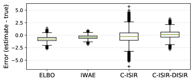
Figure 5: Boxplot representation of the error of different estimators for the gradient w.r.t. one of the weights of the PPCA model.

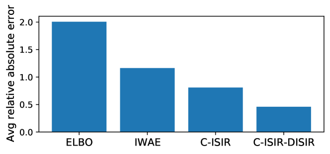
Figure 6: Relative error (in absolute value) for the PPCA model, averaged over all components of the gradient.

D.2 Experimental Setup for the VAE

Binarized MNIST.  For binarized MNIST, the model is $p_{\theta}(x,z)=\mathcal{N}(z;0,I)p_{\theta}(x\,|\,z)$, where $p_{\theta}(x\,|\,z)$ is a product of Bernoulli distributions whose parameters are obtained as the output of a neural network with $2$ hidden layers of $200$ hidden units each and ReLU activations (the third layer is the output layer and has sigmoid activations). We set the distribution $q_{\phi}(z\,|\,x)$ as a fully factorized Gaussian, and the encoder network has an analogous architecture (in this case, the output layer implements a linear transformation for the variational means and a softplus transformation for the standard deviations). The RMSProp learning rate is $5\times 10^{-4}$ and the batchsize is $100$.

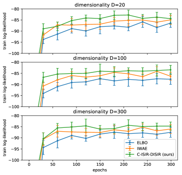
Figure 7: Train log-likelihood on a VAE fitted on binarized MNIST. The estimator from Algorithm 4 provides better performance for multiple values of the dimensionality $D$.

Fashion-MNIST and CIFAR-10.  We define the likelihood $p_{\theta}(z\,|\,x)$ using a mixture of $10$ discretized logistic distributions [Salimans et al., 2017].

For fashion-MNIST, we use the same encoder and decoder architecture as for binarized MNIST described above (except for the output layer of the decoder, which implements a linear transformation for the location parameters, a softplus transformation for the scale parameters, and a softmax transformation for the mixture weights).

For CIFAR-10, we use convolutional networks instead. The decoder consists of a fully connected layer with hidden size $16\times 16\times 1$ and ReLu activations, followed by three convolutional layers with $200$, $50$, and $30$ channels (the filter size is $4\times 4$ with stride of $2$) and ReLu activations (except for the last layer). The encoder network has three convolutional layers with $64$, $128$, and $512$ channels, followed by a fully connected hidden layer with output size $128$ and by the output layer, which is the same as for fashion-MNIST.

The RMSProp learning rate is $10^{-4}$, and the batchsize is $100$ for fashion-MNIST and $50$ for CIFAR-10.

D.3 Train Log-Likelihood on Binarized MNIST

Figure 7 shows (an estimate of) the evolution of the train log-likelihood for the VAE fitted on binarized MNIST for different values of the dimensionality $D$.

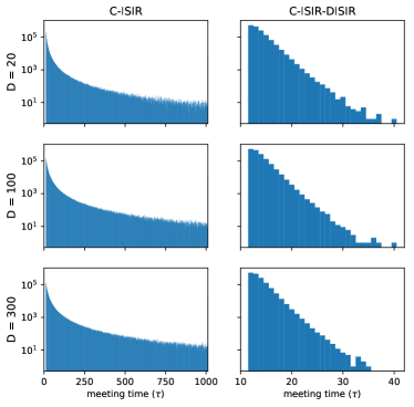
Figure 8: Histograms of the meeting time for a VAE fitted on binarized MNIST. The histograms corresponding to C-ISIR have significantly heavier tails, which results in higher computational complexity of the overall estimator.

D.4 Histograms of the Meeting Time

Figure 8 shows the histograms of the meeting time for the experiment on binarized MNIST from Section 6.2. The meeting time behaves similarly across different values of the dimensionality $D$, although the histogram gets heavier-tailed for C-ISIR when $D$ increases.