Deep Distributional Time Series Models and the Probabilistic Forecasting of Intraday Electricity Prices

Nadja Klein is Assistant Professor of Applied Statistics and Emmy Noether Research Group Leader in Statistics and Data Science at Humboldt-Universität zu Berlin; Michael Stanley Smith is Professor of Management (Econometrics) at Melbourne Business School, University of Melbourne; David J. Nott is Associate Professor of Statistics and Applied Probability at National University of Singapore. Correspondence should be directed to Prof. Dr. Nadja Klein at Humboldt Universität zu Berlin, Unter den Linden 6, 10099 Berlin. Email: nadja.klein@hu-berlin.de.

Acknowledgments: Nadja Klein was supported by the Deutsche Forschungsgemeinschaft (DFG, German research foundation) through the Emmy Noether grant KL 3037/1-1. David Nott is affiliated with the Operations Research and Analytics Research cluster at the National University of Singapore. The authors thank Sonnia Fuenteseca for research assistance in constructing the demand forecast data used in Section 6, and Patrick McDermott and Chris Wikle for sharing their code.

Recurrent neural networks (RNNs) with rich feature vectors of past values can provide accurate point forecasts for series that exhibit complex serial dependence. We propose two approaches to constructing deep time series probabilistic models based on a variant of RNN called an echo state network (ESN). The first is where the output layer of the ESN has stochastic disturbances and a shrinkage prior for additional regularization. The second approach employs the implicit copula of an ESN with Gaussian disturbances, which is a deep copula process on the feature space. Combining this copula with a non-parametrically estimated marginal distribution produces a deep distributional time series model. The resulting probabilistic forecasts are deep functions of the feature vector and also marginally calibrated. In both approaches, Bayesian Markov chain Monte Carlo methods are used to estimate the models and compute forecasts. The proposed models are suitable for the complex task of forecasting intraday electricity prices. Using data from the Australian National Electricity Market, we show that our deep time series models provide accurate short term probabilistic price forecasts, with the copula model dominating. Moreover, the models provide a flexible framework for incorporating probabilistic forecasts of electricity demand as additional features, which increases upper tail forecast accuracy from the copula model significantly.

Keywords: Copula, density forecasts, echo state network, electricity price forecasting, marginal calibration, Markov chain Monte Carlo, recurrent neural network.

1 Introduction

Deep models with rich feature vectors are often very effective in problems which require accurate forecasts (Goodfellow et al., 2016). These include financial applications, such as predicting equity risk premiums and returns (Feng et al., 2018, Gu et al., 2020b, a) and bond returns (Bianchi et al., 2020). Another financial application where deep models have high potential is the forecasting of intraday electricity prices. Electricity prices exhibit a strong and complex nonlinear serial dependence, quite unlike security prices, and accounting for this is key to obtaining accurate forecasts (Nowotarski and Weron, 2018, Manner et al., 2019). Shallow neural networks (NNs) (Amjady, 2006, Mandal et al., 2007), and more recently deep neural networks (DNNs) (Lago et al., 2018, Ugurlu et al., 2018), have been shown to capture these nonlinearities well and produce accurate point forecasts. However, it is the accurate forecasting of the entire distribution of prices—variously called probabilistic, density or distributional forecasting—that is important for both market operators and participants. Yet, to date, probabilistic forecasts of electricity prices using DNNs are rare. In this paper, we propose a number of time series probabilistic forecasting models that exploit and extend state-of-the-art deep models, and apply them to data from the Australian market.

Day-ahead wholesale electricity markets operate throughout the world, including in the U.S. and Europe. In these markets, generators and distributors bid for sale and purchase of electricity at an intraday resolution in an auction one day prior to transmission. The auction clearing price is widely called the electricity spot price; see Kirschen and Strbac (2018) for an introduction to such markets. Accurate price forecasts at an intraday resolution, one or more days ahead, are central to both the efficient operation of the market and profitability of participants. Particularly important are probabilistic forecasts of price, not just the mean, variance or other moments. This is because overall profitability of market participants is strongly affected by prices in the tails, which are very heavy in most wholesale markets.

Recurrent neural networks (RNNs) are DNNs tailored to capture temporal behavior, and are suitable for forecasting nonlinear time series (Goodfellow et al., 2016, Ch.10). However, RNNs typically have a very large number of hidden weights and are difficult to train and tune. Therefore, we use a variant of RNNs called echo state networks (ESNs) (Jaeger, 2007, Lukoševičius and Jaeger, 2009), that are flexible and employ a form of regularization that makes them scalable to long series and computationally stable. We build statistical time series models based on ESNs using two approaches. The first extends that of Chatzis and Demiris (2011) and McDermott and Wikle (2017, 2019), who use ESNs within statistical models, with the output layer coefficients of the hidden state vector estimated using Bayesian methods. In our work we include a shrinkage prior for these coefficients to provide additional regularization, along with three different additive error distributions for the output layer: Gaussian, skew-normal and skew-$t$.

Our second approach is the main methodological contribution of the paper. It uses the implicit copula of the time series vector from a Gaussian probabilistic ESN of the type described above. By an “implicit copula” we mean the copula that is implicit in a multivariate distribution and that is obtained by inverting the usual expression of Sklar’s theorem as in Nelsen (2006, Sec. 3.1). This implicit copula is both a deep function of the feature vector, and also a “copula process” with the same dimension as the time series vector. We combine our proposed copula with a non-parametrically estimated marginal distribution for electricity prices, producing a time series model that captures the complex serial dependence in the series. An accurate estimate of the marginal distribution ensures “marginal calibration”, which is where the long run average of the predictive distributions of the time series variable matches its observed margin (Gneiting et al., 2007, Gneiting and Katzfuss, 2014). Importantly, the entire predictive distribution from the copula model is a deep function of the feature vector. We note that our copula model extends the deep distributional regression methodology of Klein et al. (2020) to deep distributional time series and ESNs.

In both our deep time series models the feature vector includes a rich array of past series values and possibly other variables. To regularize these, ESNs use sparse and randomly assigned fixed weights for the hidden layers of the DNN. For each of $K$ random configurations of weights, Markov chain Monte Carlo (MCMC) is used to estimate the statistical model and compute Bayesian predictive distributions. The probabilistic forecasts are then ensembles of these predictive distributions over the $K$ configurations of weights. We show in our empirical work that this ensemble provides for accurate uncertainty quantification.

We use our deep time series models to forecast intraday electricity prices in the Australian National Electricity Market (NEM). The NEM is one of the earliest established wholesale markets (in 1998), comprises approximately 1% of all Australian economic output, provides publicly available data, and has a design that is typical of other day-ahead markets. It has five regional price series for which forecasting has been much studied; see Ignatieva and Trück (2016), Smith and Shively (2018), Manner et al. (2019) and Han et al. (2020) for overviews. Using a feature vector with lagged prices from all five regions, we compute predictions at the half-hourly resolution for a 24 hour horizon over an eight month validation period during 2019. Serinaldi (2011), Gianfreda and Bunn (2018) and Narajewski and Ziel (2020) show the ‘generalized additive models for location, scale and shape’ (GAMLSS) methodology of Rigby and Stasinopoulos (2005) applied to time series allows for the accurate modeling and forecasting of electricity prices, and we employ this as a benchmark. Using contemporary metrics, the probabilistic ESN with skew-$t$ errors produces more accurate point and probabilistic forecasts than ESNs with either Gaussian or skew-normal errors, and also the GAMLSS benchmark. However, the deep copula model produces substantially more accurate probabilistic forecasts, including in both tails, and its forecasts have superior coverage. Thus, marginal calibration also improves calibration of the (conditional) predictive distributions.

Participants in the NEM are provided with probabilistic forecasts of electricity demand by the system operator. Recent studies (Ziel and Steinert, 2016, Shah and Lisi, 2020) suggest that using accurate demand forecasts may further improve time series forecasts of the distribution of price. An advantage of deep models is that additional predictors are easily included in a flexible fashion as extra elements in the feature vector. We do so here using three quantiles of the 24 hour ahead demand forecasts, and find this increases forecast accuracy of the upper tail of the price distribution, but only when using the deep copula model. Accurate forecasting of the upper tail of electricity prices impacts the profitability of participants substantially (Christensen et al., 2012).

The paper is organized as follows. Sec. 2 provides an overview of electricity markets and price forecasting, with a focus on the NEM. Sec. 3 outlines ESNs, their probabilistic extension using additive disturbances, and Bayesian methods for their estimation and prediction. Sec. 4 outlines the implicit copula process and the proposed deep distributional time series model. Sec. 5 compares the deep time series and benchmark model forecasts, Sec. 6 considers the inclusion of demand forecast data, and Sec. 7 concludes. The Web Appendix (“WA” hereafter) provides key algorithms, computational details and additional empirical results.

2 Electricity Markets, Price Forecasting and Data

2.1 Wholesale markets

Wholesale electricity markets include the European Power Exchange, mutiple regional markets in the U.S. (such as the PJM interconnection and the Southwest Power Pool), and national markets in many countries including Australia, Chile and Turkey. While the designs of these markets differ, they are largely “day-ahead” markets where generators and distributors place bids for the sale and purchase of electricity at an intraday resolution up to one day prior to transmission (or “dispatch”). The market is cleared at a wholesale spot price that reflects the marginal cost of supply at each intraday period. Prices also vary at different geographic reference nodes, creating multiple related price series. Markets are overseen by system operators, which match generation with short-term demand forecasts, impose constraints to ensure system stability (i.e. avoid load-shedding or blackouts), and enforce any price caps; see Kirschen and Strbac (2018) for an overview of wholesale markets.

Central to the operation of day-ahead markets is the intraday electricity spot price. For market participants accurate short-term forecasts of the price are key to profitability. Because electricity is a flow commodity with a high cost of storage, arbitrage opportunities are limited. This fact, along with the complexities of transmission and that short-run demand is inelastic with respect to price, means that prices exhibit unique stylized characteristics; see Knittel and Roberts (2005), Karakatsani and Bunn (2008), Panagiotelis and Smith (2008) and Weron (2014) for summaries of these. From a time series perspective, this includes strong and complex nonlinear serial dependence, while from a distributional perspective prices have very heavy tails, skew and often multiple modes that correspond to different regimes (Janczura and Weron, 2010) and economic equilibria (Smith and Shively, 2018) .

2.2 Electricity price forecasting

Many methods have been used for short-term forecasting of electricity spot prices; see Weron (2014) and Nowotarski and Weron (2018) for recent overviews of point and probabilistic forecasting methods, respectively. In the machine learning literature, while shallow neural networks (NNs) have long been popular for forecasting electricity prices, DNNs have the potential to produce more accurate forecasts. For example, Lago et al. (2018) and Ugurlu et al. (2018) both found that RNN models provide more accurate point forecasts than a range of benchmark models. However, most previous usages of shallow and deep NNs have focused on point forecasts of prices, and only in a few cases also quantify predictive uncertainty using bootstrap or other Monte Carlo methods (Rafiei et al., 2016).

In contrast, a number of other methods have been used to construct probabilistic forecasts (Misiorek et al., 2006, Panagiotelis and Smith, 2008, Huurman et al., 2012, Bunn et al., 2016). One particularly promising avenue is to extend distributional regression methods to time series forecasting. For example, Gianfreda and Bunn (2018) and Narajewski and Ziel (2020) do so for German electricity prices using exogenous covariates, and Serinaldi (2011) does so for Californian and Italian electricity prices using historical prices and other variables. These papers report more accurate probabilistic forecasts. In Sec. 4 we develop a copula-based model that exploits the accuracy exhibited by deep models within a distributional time series forecasting setting, thereby combining the advantages of both approaches.

Copulas have become increasingly popular in time series models of electricity prices because they can capture complex dependence, while also allowing for highly flexible margins. Smith et al. (2012), Ignatieva and Trück (2016), Manner et al. (2016), Pircalabu and Benth (2017) and Manner et al. (2019) use low-dimensional copulas to capture cross-sectional dependence between regional prices, price spikes and other energy series in interconnected power systems, while Smith and Shively (2018) use high-dimensional copulas to capture both serial and cross-sectional dependence jointly for multiple regional prices. However, these studies all employ copulas that are very different to the copula process proposed here.

2.3 Australian electricity prices

Electricity generation in the NEM is an important component of economic activity, with 19.4bn Australian dollars of turnover during the 2018-2019 financial year (Australian Energy Regulator, 2019). Operations in the NEM are managed by the Australian Electricity Market Operator (AEMO), and since April 2006 it has had five regions which correspond to the power systems in the states of New South Wales (NSW), Queensland (QLD), Victoria (VIC), South Australia (SA) and Tasmania (TAS). Separate prices are set at a central location (or “node”) in each region, although they are dependent because the state-based power systems are interconnected by high voltage direct current lines.

Participating utilities place bids for the purchase (by distributors) and sale (by generators) of electricity at five minute intervals up to one day prior to dispatch. The trading price is the average clearing price for this auction over six consecutive five minute periods, so that it is observed at a half-hourly resolution. Re-bidding of prices is allowed before dispatch, although not the amount of energy. Price forecasting in the NEM has been studied extensively, with contributions by Higgs (2009), Panagiotelis and Smith (2008), Nowotarski et al. (2013), Ignatieva and Trück (2016), Rafiei et al. (2016), Smith and Shively (2018), Apergis et al. (2019) and Manner et al. (2019) among others. Intraday forecasts over a horizon of 24 hours are used by market participants to develop effective strategies for bidding, re-bidding and managing risk. In our study, we employ the half-hourly trading prices (measured in Australian dollars per MW/h) observed during 2019 in the five regions of the NEM. Prices can be negative for short periods (when it is more cost-effective to sell into the market at a loss, rather than ramp down generation temporarily) although the floor price is -$1,000. There is also a maximum price that is adjusted annually on 1 July, which was $14,500 prior to 1 July 2019 and $14,700 afterwards.

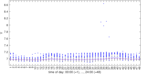
Figure 1: Boxplots of the logarithm of electricity prices in the NSW region by hour.

Fig. A in the WA plots prices in NSW during four weeks corresponding to the four seasons, illustrating the strong heterogeneity based on the time of day, day of the week and season. Table B in the WA provides a summary of the prices in each region. These have extreme positive skew, so that we follow most previous studies and work with the logarithm of price $Y=\log(\mbox{Price}+1001)$. The addition of 1001 accounts for the minimum price, at which $Y=0$. It is straightforward to construct density forecasts of the nominal price from those of $Y$ using the Jacobian of the transformation. Fig. B in the WA plots histograms of the five price series, along with (bounded) kernel density estimates (KDEs), showing that even the distribution of $Y$ is both asymmetric and heavy-tailed for each series. Figure 1 gives boxplots of $Y$ for NSW (which is the region with the most energy demand), broken down by hour of the day. It shows that the entire distribution varies substantially over the day. Equivalent plots for the day of the week, and month of the year, (see the WA) also reveal similar heterogeneity in the distribution of prices.

3 Deep Time Series

RNNs represent complex temporal relationships between variables by allowing cycles and sequences in their hidden layers. However, RNNs are typically computationally expensive to estimate and can be numerically unstable for long series (Pascanu et al., 2013), both of which are issues here. One way to address this is to employ a variant called an Echo State Network (ESN) that decreases the number of weights that need to be trained (Jaeger, 2007). The key idea of ESNs is to only adapt the output layer in training, while keeping the weights of recurrent and input connections fixed yet randomly assigned. Such an approach is called a ‘reservoir computing’ method (Lukoševičius and Jaeger, 2009), because it establishes a multiple linkage hidden reservoir which can be of much higher dimension than the input, providing a lot of flexibility at a lower computational cost. However, classical ESNs and many of its extensions rarely consider uncertainty quantification, and in this section we outline probabilistic ESNs that do so. The approach is extended in Sec. 4 to allow for marginal calibration of the data distribution using a deep copula construction.

3.1 Gaussian probabilistic ESN

3.1.1 Specification

We first specify the ensemble ESN proposed for spatio-temporal data by McDermott and Wikle (2017). For series with highly nonlinear dependence, these authors demonstrate that allowing the response equation to depend on the hidden states quadratically in an ESN can increase predictive accuracy, which we also find for the electricity price series examined here. Let $\{Y_{t}\}$ be a stochastic process, then the ESN with Gaussian disturbances $\varepsilon_{t}\sim\mathcal{N}(0,\sigma^{2})$ takes the following form for $t\geq 1$:

Response Equation: $$Y_{t} =\beta_{0}+\text{\boldmath$h$}_{t}^{\prime}\text{\boldmath$\beta$}_{1}+(\text{\boldmath$h$}_{t}^{\prime})^{\circ 2}\text{\boldmath$\beta$}_{2}+\varepsilon_{t}\,,$$ (1)

Hidden State Equation: $$\text{\boldmath$h$}_{t} =(1-\kappa)\text{\boldmath$h$}_{t-1}+\kappa\tilde{\text{\boldmath$h$}}_{t}$$

$$\tilde{\text{\boldmath$h$}}_{t} =g_{h}\left(\frac{\delta}{\lambda_{V}}V\text{\boldmath$h$}_{t-1}+U\text{\boldmath$x$}_{t}\right)\,.$$

Here, $\text{\boldmath$x$}_{t}$ is an $n_{x}$-dimensional feature vector that includes unity for an intercept term, $\text{\boldmath$h$}_{t}$ is a $n_{h}$-dimensional hidden state vector, ‘$\circ 2$’ denotes the element-wise square of a matrix, $V,U$ are $(n_{h}\times n_{h})$ and $(n_{h}\times n_{x})$ matrices of hidden layer weights, and $g_{h}$ is an activation function, set here to $g_{h}(x)=\tanh(x)$. The parameter $0<\kappa\leq 1$ and is known as the “leaking rate”. Similar to McDermott and Wikle (2017) we set $\kappa=1$ after having checked that predictive performance is not improved by setting $\kappa<1$, so that $\tilde{\text{\boldmath$h$}}_{t}=\text{\boldmath$h$}_{t}$. The feature vector $\text{\boldmath$x$}_{t}$ contains past values of both the response and other series, which we specify in Sec. 5. The response $Y_{t}$ is a nonlinear function not only of $\text{\boldmath$x$}_{t}$, but also of all previous values $\text{\boldmath$x$}_{1},\ldots,\text{\boldmath$x$}_{t-1}$, so the stochastic process is not Markov.

The constant $\lambda_{V}$ is the largest eigenvalue of $V$, and $0<\delta<1$ a scaling parameter, so that $(\delta/\lambda_{V})V$ has spectral radius less than one. A spectral radius greater than one can result in unstable behavior in the latent states (Lukoševičius and Jaeger, 2009). We follow McDermott and Wikle (2017) and set $\delta=0.35$ and $n_{h}=120$, although we found the forecasting results to be insensitive to variations in these settings.

The elements of the matrices $V=\{v_{il}\},U=\{u_{ij}\}$ are assumed to be random, and distributed independently from mixtures of a uniform distribution and a point mass at zero. If $\mathcal{U}(a,b)$ denotes a uniform distribution over domain $(a,b)$, $\mathcal{B}(\pi)$ denotes a beta distribution with mean $\pi$, and $\delta_{0}$ is the Dirac function at zero, then the elements

$$v_{il} = \gamma_{il}^{v}\mathcal{U}(-a_{v},a_{v})+(1-\gamma_{il}^{v})\delta_{0}\,,\;\;\gamma_{il}^{v}\sim\mathcal{B}(\pi_{v})\,,$$

$$u_{ij} = \gamma_{ij}^{u}\;\mathcal{U}(-a_{u},a_{u})+(1-\gamma_{ij}^{u})\delta_{0}\,,\;\;\gamma_{ij}^{u}\sim\mathcal{B}(\pi_{u})\,.$$ (2)

We follow McDermott and Wikle (2017) and set $a_{v}=a_{u}=\pi_{v}=\pi_{u}=0.1$ after having checked the predictive performance under several alternative settings.

Consider $T$ time series observations $\text{\boldmath$Y$}=(Y_{1},\ldots,Y_{T})^{\prime}$ of the stochastic process with corresponding $(T\times n_{x})$ matrix of feature values $X=[\text{\boldmath$x$}_{1}|\cdots|\text{\boldmath$x$}_{T}]^{\prime}$. Denote $\text{\boldmath$\xi$}=\{V,U,\kappa,\delta\}$, $H_{\xi}(X)=[\text{\boldmath$h$}_{1}|\cdots|\text{\boldmath$h$}_{T}]^{\prime}$ as the $(T\times n_{h})$ matrix of hidden state values, $B_{\xi}(X)=[\text{\boldmath$\iota$},H_{\xi}(X)|H_{\xi}(X)^{\circ 2}]$, $\iota$ as a vector ones, and $\text{\boldmath$\beta$}=(\beta_{0},\text{\boldmath$\beta$}_{1}^{\prime},\text{\boldmath$\beta$}_{2}^{\prime})^{\prime}$. Then (LABEL:eq:ESN) can be written as the linear model

$$\bm{Y}=B_{\xi}(X)\text{\boldmath$\beta$}+\text{\boldmath$\varepsilon$}\,,\;\;\mbox{ }\text{\boldmath$\varepsilon$}=(\varepsilon_{1},\ldots,\varepsilon_{T})^{\prime}\sim\mathcal{N}(\mathbf{0},\sigma^{2}I).$$ (3)

Given $\xi$, $X$ and $\text{\boldmath$h$}_{0}=\bm{0}$, the hidden state matrix $H_{\xi}(X)$ is known without error as the hidden state vectors can be computed recursively. Only $\beta$ and $\sigma^{2}$ (which we refer to as model parameters) require estimation, for which we use their Bayesian posterior distribution. Differing from McDermott and Wikle (2017), we regularize $\beta$ by adopting the shrinkage prior

$$\text{\boldmath$\beta$}|\tau^{2}\sim\mathcal{N}(\mathbf{0},P(\tau^{2})^{-1})\,,\;\sigma^{2}\sim\mathcal{IG}(a,b)\,,$$ (4)

where $\mathcal{IG}$ denotes an Inverse Gamma distribution. We found a ridge prior with $P(\tau^{2})=\tau^{2}I$, and hyper-prior $\tau^{2}\sim\mathcal{IG}(\tilde{a},\tilde{b})$ with $a=b=\tilde{a}=\tilde{b}=0.001$ to work well. The posterior of the model parameters $\text{\boldmath$\vartheta$}=(\text{\boldmath$\beta$},\sigma^{2},\tau^{2})$ of this regularized linear model can be computed using the standard MCMC sampler at Algorithm 1 in Part A of the WA.

3.1.2 Probabilistic forecasts

Most implementations of ESNs only draw a single set of weights from (2). Here, we follow McDermott and Wikle (2017, 2019) and simulate $K=100$ matrices $\{V^{k},U^{k}\,;k=1,\ldots,K\}$ from (2). An ensemble is then used to integrate over $U,V$ when constructing the probabilistic forecasts. If $\text{\boldmath$\xi$}^{k}=\{V^{k},U^{k},\kappa,\delta\}$, then the density forecast of $Y_{T+h}$ at time $T$ for each point $h=1,\ldots,h_{1}$ in the forecast horizon is the ensemble

$$f_{T+h|T}(y_{T+h})\equiv\frac{1}{K}\sum_{k=1}^{K}p^{k}(y_{T+h}|X,\text{\boldmath$y$})\,,$$ (5)

where the subscript notation indicates $f_{T+h|T}$ is conditional on the filtration at time $T$.

The density $p^{k}$ in (5) is the Bayesian posterior predictive density computed for configuration $\text{\boldmath$\xi$}^{k}$ as follows. Let $X_{(t)}\equiv[\text{\boldmath$x$}_{1}|\cdots|\text{\boldmath$x$}_{t}]^{\prime}$, then

$$p^{k}(y_{T+h}|X,\text{\boldmath$y$}) = \int\int p(y_{T+h}|X_{(T+h)},\text{\boldmath$\vartheta$})p(\text{\boldmath$x$}_{T+2},\ldots,\text{\boldmath$x$}_{T+h}|\text{\boldmath$\vartheta$},X,\text{\boldmath$y$})$$ (6)

$$\;\;\;\;\;\;\;\;p(\text{\boldmath$\vartheta$}|X,\text{\boldmath$y$})\mathrm{d}\text{\boldmath$x$}_{T+2}\cdots\mathrm{d}\text{\boldmath$x$}_{T+h}\,\mathrm{d}\text{\boldmath$\vartheta$}\,,$$

which is an integral over any unobserved feature values and the model parameter posterior. From (LABEL:eq:ESN), the first term in the integrand is the density of a $\mathcal{N}(\text{\boldmath$h$}_{T+h}^{\prime}\text{\boldmath$\beta$}_{1}+(\text{\boldmath$h$}_{T+h}^{\prime})^{\circ 2}\text{\boldmath$\beta$}_{2},\sigma^{2})$ distribution, where $\text{\boldmath$h$}_{T+h}$ is computed through the recursion of the hidden state equation (therefore $\text{\boldmath$h$}_{T+h}$ is a deep function of $\text{\boldmath$x$}_{1},\ldots,\text{\boldmath$x$}_{T+h}$). The outer integral in $\vartheta$ can be evaluated by averaging over draws from the posterior $p(\text{\boldmath$\vartheta$}|X,\text{\boldmath$y$})$ obtained from running the MCMC sampler. However, plugging in the posterior mean $E(\text{\boldmath$\vartheta$}|X,\text{\boldmath$y$})$ computed from the Monte Carlo sample is much faster, yet can be almost as accurate, so we follow this approach.

In our empirical work $\text{\boldmath$x$}_{t}$ contains past values of both the focal price and the other four regional prices, so that $\text{\boldmath$x$}_{1},\ldots,\text{\boldmath$x$}_{T+1}$ are observed at or before time $T$. However, some elements of $\text{\boldmath$x$}_{T+2},\ldots,\text{\boldmath$x$}_{T+h}$ are unobserved, and the integrals over these feature vectors in (6) are with respect to their unobserved elements only. The integrals are computed in a Monte Carlo manner by simulating all five series values sequentially from their predictive distributions. Algorithm 2 in Part B of the WA simulates from the ensemble density (5) for all five regional price series and over each time point in the forecast horizon.

3.2 Skew $t$ probabilistic ESN

Adopting Gaussian disturbances to the output layer at (LABEL:eq:ESN) is inconsistent with the strong asymmetry in the empirical distribution of (the logarithm of) prices. Thus, we also consider the skew-$t$ distribution of Azzalini and Capitanio (2003) with location zero for the disturbances, with density $p(\varepsilon_{t};\omega^{2},\alpha,\nu)=\frac{2}{\omega}t_{\nu}\left(\frac{\varepsilon_{t}}{\omega}\right)T_{\nu+1}\left(\frac{\alpha\varepsilon_{t}}{\omega}\sqrt{\frac{\nu+1}{\nu+x_{\varepsilon_{t}}^{2}}}\right)$, where $t_{\nu}$ and $T_{\nu}$ are the student $t$ density and distribution functions. The parameters $\omega^{2},\alpha,\nu$ are scale, skew and degrees of freedom parameters, respectively, and we write $\varepsilon_{t}\sim\mathcal{ST}(0,\omega^{2},\alpha,\nu)$. When $\nu>30$ the density is effectively that of a skew-normal distribution, whereas when $\alpha=0$ it is that of a $t$ distribution. We fix values of $\nu$, and use the prior at (4) for $\beta$, so that the model parameters are $\{\text{\boldmath$\beta$},\tau^{2},\omega^{2},\alpha\}$.

Bayesian estimation of the model parameters uses a conditionally Gaussian representation of the skew-$t$. This introduces latent variables $\zeta_{t},w_{t}$, and expresses $\varepsilon_{t}$ conditional on these values as $\varepsilon_{t}=\psi\zeta_{t}+\epsilon_{t}$, where

$$\epsilon_{t}|w_{t}\sim\mathcal{N}(0,\sigma^{2}/w_{t})\,,\,w_{t}\sim\mathcal{G}\left(\frac{\nu}{2},\frac{\nu}{2}\right)\,,\,\zeta_{t}|w_{t}\sim\mathcal{TN}_{[0,\infty)}\left(0,1/w_{t}\right)\,,$$

$\mathcal{G}$ denotes a Gamma distribution, $\mathcal{TN}_{[0,\infty)}$ is a Gaussian truncated to $[0,\infty)$, and $\{\alpha,\omega\}$ are re-parameterized as $\{\psi,\sigma\}$ with $\psi=\alpha\sigma$ and $\sigma^{2}=\omega^{2}-\psi^{2}$. Integrating out $\zeta_{t},w_{t}$ recovers the skew-$t$ distribution $\varepsilon_{t}\sim\mathcal{ST}(0,\omega^{2},\alpha,\nu)$. Following Frühwirth-Schnatter and Pyne (2010), the hyperpriors are $\psi\sim\mathcal{N}(0,D_{0})$, $\sigma^{2}\sim\mathcal{IG}(c_{0},C_{0})$ and $\tau^{2}\sim\mathcal{IG}(b_{0},B_{0})$, with constants $D_{0}=1$, $c_{0}=2.5$, $b_{0}=1$, $B_{0}=0.005$, $C_{0}=0.5s_{y}^{2}$ and $s_{y}^{2}$ denoting the sample variance of the response $Y_{t}$.

Given $\xi$, the re-parameterized model parameters $\text{\boldmath$\vartheta$}=\{\text{\boldmath$\beta$},\tau^{2},\psi,\sigma^{2}\}$ are estimated using their Bayesian posterior computed by an MCMC sampler that generates $\text{\boldmath$\zeta$}=(\zeta_{1},\ldots,\zeta_{T})^{\prime}$ and $\bm{w}=(w_{1},\ldots,w_{T})^{\prime}$, similar to those proposed by Panagiotelis and Smith (2008) and Frühwirth-Schnatter and Pyne (2010). As with the Gaussian probabilistic ESN, prediction is based on Monte Carlo draws from the ensemble density at (5) produced using a minor adjustment of Algorithm 2. Details are given in Part B of the WA.

4 Deep Distributional Time Series

While the deep time series models in Sec. 3 provide probabilistic forecasts they have two drawbacks: (i) the feature vector only affects the mean of the response equation at (LABEL:eq:ESN), and (ii) the density forecasts are not calibrated in any manner. In this section, a copula model is outlined that is a deep distributional time series model in which the feature vector affects the entire predictive distribution and the probabilistic forecasts are marginally calibrated.

4.1 Marginal calibration

Gneiting et al. (2007) discuss different forms of calibration of density forecasts, including predictive marginal calibration, which is defined as follows. For $t=T+1,\ldots,\infty$, assume a future observation of $Y_{t}$ has true distribution $H_{t|T}(y)$ and forecast distribution $F_{t|T}(y)$, where the subscript indicates that both distributions are conditional on the filtration at time $T$. Then, if $\bar{H}(y)\equiv\lim_{h_{1}\rightarrow\infty}\left\{\frac{1}{h_{1}}\sum_{h=1}^{h_{1}}H_{T+h|T}(y)\right\}$ and $\bar{F}(y)\equiv\lim_{h_{1}\rightarrow\infty}\left\{\frac{1}{h_{1}}\sum_{h=1}^{h_{1}}F_{T+h|T}(y)\right\}$, the forecast distributions are called marginally calibrated if and only if $\bar{F}(y)=\bar{H}(y)$.

Gneiting et al. (2007) highlight that because $H_{t|T}$ is unknown for $t>T$, marginal calibration can be assessed in practice by comparing the empirical distribution function over the forecast horizon to the average of the corresponding distributional forecasts. In a study with a moving window (such as ours) and forecast origins $T=T_{\mbox{\tiny start}},\ldots,T_{\mbox{\tiny finish}}$, there are a total of $N=T_{\mbox{\tiny finish}}-T_{\mbox{\tiny start}}+1$ sets of forecasts. Averaging over these and the forecast horizon of length $h_{1}$, gives

$$\hat{H}(y)=\frac{1}{Nh_{1}}\sum_{T=T_{\mbox{\tiny start}}}^{T_{\mbox{\tiny finish}}}\sum_{t=T+1}^{T+h_{1}}\mathcal{I}(y_{t}\leq y)\,,\mbox{ and }\hat{F}(y)=\frac{1}{Nh_{1}}\sum_{T=T_{\mbox{\tiny start}}}^{T_{\mbox{\tiny finish}}}\sum_{t=T+1}^{T+h_{1}}F_{t|T}(y)\,,$$ (7)

where $\mathcal{I}(X)$ is an indicator function equal to one if $X$ is true, and zero otherwise. The closer $\hat{F}$ is to $\hat{H}$, the greater evidence for predictive marginal calibration.

4.2 Copula model

We adopt a copula model for the joint distribution of $\bm{Y}_{(t)}=(Y_{1},\ldots,Y_{t})^{\prime}$, conditional on $X_{(t)}=[\text{\boldmath$x$}_{1}|\cdots|\text{\boldmath$x$}_{t}]^{\prime}$ and weight configuration $\xi$, with the density decomposition

$$p(\text{\boldmath$y$}_{(t)}|X_{(t)},\text{\boldmath$\xi$})=c_{\mbox{\tiny ESN}}(F_{Y}(y_{1}),\ldots,F_{Y}(y_{t})|X_{(t)},\text{\boldmath$\xi$})\prod_{s=1}^{t}p_{Y}(y_{s})\,,\;\mbox{ for }t\geq 2\,,$$ (8)

where $\text{\boldmath$y$}_{(t)}=(y_{1},\ldots,y_{t})^{\prime}$ and $\text{\boldmath$u$}_{(t)}=(u_{1},\dots,u_{t})^{\prime}$. The deep copula process has $t$-dimensional density $c_{\mbox{\tiny ESN}}(\text{\boldmath$u$}_{(t)}|X_{(t)},\text{\boldmath$\xi$})$ specified below in Sec. 4.3. The density $p_{Y}$ and corresponding distribution function $F_{Y}$ in (8) are time invariant, and are estimated non-parametrically from the training data. This ensures in-sample marginal calibration, which will extend to predictive calibration whenever the series is stationary.

We stress that even though in (8) the distribution $Y_{t}|\text{\boldmath$x$}_{t}$ is assumed marginally invariant with respect to $\text{\boldmath$x$}_{t}$, the distribution $\bm{Y}_{(t)}|X_{(t)}$ is still related to the matrix of feature vector values $X_{(t)}$ though the joint distribution. A consequence is that for $t>T$ the predictive density of $Y_{t}$ can be heavily dependent on the feature vector $\text{\boldmath$x$}_{t}$, as outlined in Sec. 4.5.

4.3 Specification of the deep copula process

At (8) we employ an (implicit) copula process with density $c_{\mbox{\tiny ESN}}$ constructed from the joint distribution of a second stochastic process $\{\tilde{Z}_{s}\}$ that follows the Gaussian probabilistic ESN at (LABEL:eq:ESN) with $\beta$ integrated out under the prior (4). We call $\tilde{Z}_{s}$ a “pseudo-response” because it is not observed directly, but is introduced only for specification of its implicit copula. The $t$ observations $\tilde{\bm{Z}}_{(t)}=(\tilde{Z}_{1},\ldots,\tilde{Z}_{t})^{\prime}$, are conditionally distributed

$$\tilde{\bm{Z}}_{(t)}|X_{(t)},\sigma^{2},\tau^{2},\text{\boldmath$\xi$}\sim\mathcal{N}\left(\tilde{\text{\boldmath$z$}}_{(t)};\bm{0},\sigma^{2}\left(I+\frac{1}{\tau^{2}}B_{\text{\boldmath$\xi$}}(X_{(t)})B_{\text{\boldmath$\xi$}}(X_{(t)})^{\prime}\right)\right)\,,$$ (9)

with $\tilde{\text{\boldmath$z$}}_{(t)}=(\tilde{z}_{1},\ldots,\tilde{z}_{t})^{\prime}$ and the matrix $B_{\xi}(X_{(t)})$ is specified at (3), but without an intercept term (i.e. the first column of ones) because level is unidentified in a copula.

The implicit copula of a Gaussian distribution is called a Gaussian copula, and is constructed for (9) by standardizing the distribution. Let $\bm{Z}_{(t)}=(Z_{1},\ldots,Z_{t})^{\prime}=\sigma^{-1}S\tilde{\bm{Z}}_{(t)}$, where $S=\mbox{diag}(\psi_{1},\ldots,\psi_{t})$ is a diagonal scaling matrix with elements $\psi_{s}=(1+\text{\boldmath$b$}_{s}^{\prime}\text{\boldmath$b$}_{s}/\tau^{2})^{-1/2}$, and $\text{\boldmath$b$}_{s}$ is the $s$-th row of $B_{\xi}(X_{(t)})$. Then $\bm{Z}_{(t)}|X_{(t)},\sigma^{2},\tau^{2},\text{\boldmath$\xi$}\sim\mathcal{N}(\bm{0},R)$ where

$$R=S\left(I+\frac{1}{\tau^{2}}B_{\xi}(X_{(t)})B_{\xi}(X_{(t)})^{\prime}\right)S\,,$$

has ones on the leading diagonal, and is a function of $(X_{(t)},\text{\boldmath$\xi$},\tau^{2})$. Then the copula has density $c_{\mbox{\tiny ESN}}(\text{\boldmath$u$}_{(t)}|X_{(t)},\text{\boldmath$\xi$},\tau^{2})=\frac{\phi(\text{\boldmath$z$}_{(t)};\bm{0},R)}{\prod_{s=1}^{t}\phi_{1}(z_{s})}\,,$ where $z_{t}=\Phi_{1}^{-1}(u_{t})$, $\text{\boldmath$z$}_{(t)}=(z_{1},\ldots,z_{t})^{\prime}$, $\phi_{1}$ is the standard normal density, and $\phi(\cdot\,;\bm{0},R)$ is the density of a $\mathcal{N}(\bm{0},R)$ distribution. Notice that $\sigma^{2}$ does not feature in $c_{\mbox{\tiny ESN}}$, which is because implicit copulas are scale free.

Because $c_{\mbox{\tiny ESN}}$ is conditional on $X_{(t)}$, this is a Gaussian copula process on the feature space (Wilson and Ghahramani, 2010). Because the copula captures the dependence structure in $\{Z_{t}\}$, $\bm{x}_{t}$ contains past values of this process (rather than $\{Y_{t}\}$), and the equivalent processes for the other four regional electricity prices. These can be computed easily as $Z_{t}=\Phi^{-1}(F_{Y}(Y_{t}))$. We write the copula density $c_{\mbox{\tiny ESN}}$ also as a function of the unknown parameter $\tau^{2}$ and employ it in the copula model at (8).

4.4 Estimation

Given a configuration $\xi$, the only unknown copula parameter is $\tau^{2}$, for which we adopt the Weibull prior of Klein and Kneib (2016) with scale parameter $b_{\tau^{2}}=2.5$. Direct estimation using the likelihood at (8) is difficult because evaluation of $c_{\mbox{\tiny ESN}}(\text{\boldmath$u$}|X,\text{\boldmath$\xi$},\tau^{2})$ requires inversion of the matrix $R$, which is computationally infeasible for all but small sample sizes. This problem is solved by expressing the likelihood conditional on $\beta$ as follows. For a sample of size $T$, denote the observations as $\text{\boldmath$y$}\equiv\text{\boldmath$y$}_{(T)}$ and feature matrix as $X\equiv X_{(T)}$. Then the conditional likelihood is obtained by a change of variables from $\bm{y}$ to $\bm{z}=(z_{1},\ldots,z_{T})^{\prime}$, with elements $z_{t}=\Phi_{1}^{-1}(F_{Y}(y_{t}))$, so that

$$p(\text{\boldmath$y$}|X,\text{\boldmath$\beta$},\text{\boldmath$\xi$},\tau^{2})=p(\text{\boldmath$z$}|X,\text{\boldmath$\beta$},\text{\boldmath$\xi$},\tau^{2})\prod_{t=1}^{T}\frac{p_{Y}(y_{t})}{\phi_{1}(z_{t})}\\ =\phi\left(\text{\boldmath$z$};\bm{0},SB_{\text{\boldmath$\xi$}}(X)\text{\boldmath$\beta$},S^{2}\right)\prod_{t=1}^{T}\frac{p_{Y}(y_{t})}{\phi_{1}(z_{t})}\,,$$

which can be evaluated in $O(T)$ operations because $S$ is diagonal. Part C of the WA provides an MCMC sampler to generate draws from the augmented posterior of $(\text{\boldmath$\beta$},\tau^{2})$, so that $\beta$ is integrated out in a Monte Carlo manner and direct computation of $R$ is avoided.

4.5 Probabilistic forecasts

As with the probabilistic ESNs in Sec. 3, an ensemble is used to integrate over the distribution of $U,V$, so that the density forecast of $Y_{T+h}$ is again given by (5). The ensemble components $p^{k}$ (i.e. the Bayesian posterior predictive densities at (6)) are derived from the copula model where $\text{\boldmath$\vartheta$}=\{\text{\boldmath$\beta$},\tau^{2}\}$. To do so, the first term in the integrand of (6) is obtained by a change of variables from $y_{T+h}$ to $z_{T+h}=\Phi_{1}^{-1}(F_{Y}(y_{T+h}))$, so that

$$p(y_{T+h}|X_{(T+h)},\text{\boldmath$\vartheta$})=p(z_{T+h}|X_{(T+h)},\text{\boldmath$\beta$},\tau^{2})\frac{p_{Y}(y_{T+h})}{\phi_{1}(z_{T+h})}$$ (10)

$$= \frac{1}{\psi_{T+h}}\phi_{1}\left(\frac{\Phi_{1}^{-1}(F_{Y}(y_{T+h}))-\mu_{T+h}}{\psi_{T+h}}\right)\frac{p_{Y}(y_{T+h})}{\phi_{1}\left(\Phi_{1}^{-1}\left(F_{Y}(y_{T+h})\right)\right)}\,,$$

where $\mu_{T+h}=\frac{1}{\psi_{T+h}}\text{\boldmath$b$}_{T+h}\text{\boldmath$\beta$}$, $\psi_{T+h}=(1+\frac{1}{\tau^{2}}\text{\boldmath$b$}_{T+h}\text{\boldmath$b$}_{T+h}^{\prime})^{-1/2}$ and $\text{\boldmath$b$}_{T+h}=(\text{\boldmath$h$}_{T+h}^{\prime},(\text{\boldmath$h$}_{T+h}^{2})^{\prime})$ is a row vector. Notice that the entire density at (10) is a nonlinear function of the feature vector $\text{\boldmath$x$}_{T+h}$ via $\text{\boldmath$b$}_{T+h}$, so that $Y_{T+h}$ is not marginally invariant of $\text{\boldmath$x$}_{T+h}$ in the predictive distribution. As in Sec. 3.1.2, the posterior mean $E(\text{\boldmath$\vartheta$}|\text{\boldmath$y$})$ is computed from the Monte Carlo sample and plugged in for $\text{\boldmath$\beta$},\tau^{2}$ in (10). Because $\text{\boldmath$x$}_{t}$ comprises past values of $\{Z_{t}\}$ for both the focal price, and the other four regional prices, the integrals over $\text{\boldmath$x$}_{T+2},\ldots,\text{\boldmath$x$}_{T+h}$ in (6) are computed by simulating values for $Z_{T+t}$ sequentially for all five regions. Algorithm 4 in Part C of the WA generates iterates from the ensemble density for the copula model.

5 Forecasting Comparison

We illustrate the accuracy of our deep model forecasts using half-hourly price data observed during 2019 in all five regions. Competing models were fit using a moving window of three months training data, starting with the period 1 February–30 April. (We start at February, rather than January, because the input vector $\bm{x}_{t}$ defined below includes lagged values of the series.) This window was advanced monthly until the period 1 September–30 November, resulting in eight fits per model. Forecasts were constructed for a eight month evaluation period from 1 May to 31 December; a total of 245 days. The origin $T$ was advanced every half hour, and probabilistic forecasts constructed for a horizon of 24 hours (i.e. $h_{1}=48$ half-hours). When constructing forecasts during each month, the model parameter estimates obtained from the three preceding months training data were used. The reason each model was only refit eight times (rather than for every one of 11,760 half-hourly forecast origins) was to reduce the computational burden of the study. A forecast horizon up to 24 hours is necessary for the bidding and re-bidding process in the NEM.

5.1 Probabilistic forecasting models

The following four deep time series models were applied to each of the five price series:

• RNN: The Gaussian probabilistic ESN outlined in Sec. 3.1.

• RNNST: The skew-$t$ probabilistic ESN outlined in Sec. 3.2 with $\nu=7$.

• RNNSN: A skew-normal probabilistic ESN, approximated using RNNST with $\nu=30$.

• RNNC: The copula model outlined in Sec. 4 that uses the deep copula constructed from a Gaussian probabilistic ESN, along with bounded KDE margins.

For the RNN, RNNST and RNNSN, the feature vector contains the $n_{x}=271$ elements

$$\text{\boldmath$x$}_{t}=(1,\underbrace{\bm{Y}_{\mbox{\tiny{ALL}},t-1},\bm{Y}_{\mbox{\tiny{ALL}},t-2},\ldots,\bm{Y}_{\mbox{\tiny{ALL}},t-48}}_{\text{prices in previous 24 hours}},\underbrace{\bm{Y}_{\mbox{\tiny{ALL}},t-96},\bm{Y}_{\mbox{\tiny{ALL}},t-144},\ldots,\bm{Y}_{\mbox{\tiny{ALL}},t-336}}_{\text{prices at same hour 2 to 7 days previously}})^{\prime}\,,$$

where $\bm{Y}_{\mbox{\tiny{ALL}},t}=(Y_{\mbox{\tiny{NSW}},t},Y_{\mbox{\tiny{QLD}},t},Y_{\mbox{\tiny{SA}},t},Y_{\mbox{\tiny{TAS}},t},Y_{\mbox{\tiny{VIC}},t})$ is the vector of all five regional prices at hour $t$ and the first entry is the intercept. For RNNC, the $\text{\boldmath$x$}_{t}$ contains values of the transformed series $Z_{t}=\Phi_{1}^{-1}(F_{Y}(Y_{t}))$ for each of the five regions at the same lagged time points as above. The choice of inputs is motivated by previous studies (Panagiotelis and Smith, 2008, Higgs, 2009) that identify strong dependence in Australian electricity prices with those in the previous 24 hours, and at the same time during the previous seven days. Price dependence is induced by serial dependence in both supply-side factors and in electricity consumption (Smith, 2000). Complex cross-sectional serial dependence in price is also well-documented (Panagiotelis and Smith, 2008, Higgs, 2009, Ignatieva and Trück, 2016, Han et al., 2020) and is caused by inter-regional trade in electricity between the five regions.

While the deep time series models above are trained separately for each price series, the inclusion of lagged prices from all regions as elements of $\text{\boldmath$x$}_{t}$ forms five-dimensional multivariate deep times series models. From each model multi-step ahead forecast densities for the five regional prices are constructed jointly via simulation using Algorithms 2 and 5 outlined in the WA. At each forecast origin, $2000$ Monte Carlo draws from (5) are obtained for each half hour $h=1,\dots,48$ and region $r=1,\ldots,5$.

The density $p_{Y}$ was estimated for each series using the bounded KDE implemented in MATLAB function ‘ksdensity’, with bounds set equal to the admissible prices during the forecast period. These were a floor price of -$1000 ($Y_{T+h}\geq 0$), and a maximum price of $14,500 prior to 1 July ($Y_{t+h}\leq 9.582$) and $14,700 on or after that date ($Y_{t+h}\leq 9.596$). These densities are given in Fig. B in the WA. This ensures that the predictive densities from the copula model at (6) are constrained to the same range, which is important for the accurate forecasting of prices near the bounds. In contrast, density forecasts from the other models are unconstrained, and can have substantial mass outside the bounds. Thus, we simply truncate their predictive densities to the admissible price region and normalize.

In addition to our four proposed deep time series models, following  Serinaldi (2011) and Gianfreda and Bunn (2018) we also employ GAMLSS as a benchmark. In this framework the response $Y_{t}$ has a specified parametric distribution, where the parameters are modeled as flexible functions of covariates. We used the R package ‘gamlss’, but found the software unstable when the ESN output layer terms were used as covariates, and also for many of the candidate distributions supported by the package. However, the four parameter Johnson’s SU distribution with $\text{\boldmath$x$}_{t}$ as linear covariates worked well, and we include forecasts from this model. Serinaldi (2011) also found the JSU distribution to work well for electricity prices, which are a challenging series with which to calibrate models due to the frequent price spikes. Details on our GAMLSS implementation and experiments are given in Part D of the WA.

5.2 Measuring forecast accuracy

For point forecasts, the mean absolute error (MAE) and root mean square error (RMSE) are used to measure accuracy. For a univariate probabilistic forecast distribution $F$ there are a growing number of measures of accuracy, many of which are listed by Nowotarski and Weron (2018), and we compute the following four. The first is the quantile score function $\mbox{QS}_{\alpha}(F^{-1}(\alpha),y)=2({\cal I}(y<F^{-1}(\alpha))-\alpha)(\alpha-y)$, where ${\cal I}(A)=1$ if $A$ is true, and zero otherwise. This is also called the “pinball loss” (Raiffa and Schleifer, 1961, Gneiting, 2011). While the entire quantile score function is of interest, we also consider its value at $\alpha=0.05$ and $\alpha=0.95$ as measures of lower and upper tail accuracy, respectively. The second measure is the continuous ranked probability score (CRPS) (Gneiting et al., 2007) defined as $\mbox{CRPS}(F,y)=\int_{0}^{1}\mbox{QS}_{\alpha}(F^{-1}(\alpha),y)d\alpha$ for observed value $y$, where the integral is computed numerically. It is a proper scoring rule which measures overall probabilistic forecast accuracy.

The third measure is a loss function proposed by Fissler et al. (2016) that is based on the “value-at-risk” and “expected shortfall”, which are popular measures of financial tail risk for low values (i.e. financial losses). To measure tail risk associated with high values (which is the primary source of price risk in electricity markets) we employ the restatement of the loss function for the upper tail given by Nolde et al. (2017). For $Y\sim F$ and $\alpha$ close to 1, let $\mbox{EL}(\alpha)\equiv E(Y|Y\geq F^{-1}(\alpha))$ be the “expected longrise” (analogous to the expected shortfall measure of lower tail risk). Then from (Nolde et al., 2017, Prop. 3), the loss function is

$$S_{\alpha}(F,\mbox{EL},y)={\cal I}(y\geq F^{-1}(\alpha))\left(-G_{1}(F^{-1}(\alpha))+G_{1}(y)-G_{2}(\mbox{EL}(\alpha))(F^{-1}(\alpha)-y)\right)$$ (11)

$$+(1-\alpha)\left(G_{1}(F^{-1}(\alpha))-G_{2}(\mbox{EL}(\alpha))(\mbox{EL}(\alpha)-F^{-1}(\alpha))+G_{3}(\mbox{EL}(\alpha))\right)\,,$$

where $G_{1}(x)=x$ and $G_{2}(x)=G_{3}(x)=\exp(x)$. We compute this score for $\alpha=0.975$, and lower values indicate more accurate upper tail forecasts of the price distribution. The fourth and last measure is the empirical coverage of the predictive distributions at the 95% level.

For each of the first three metrics, we report the weighted average of their values over the evaluation period and over regions, with weights equal to the proportion of total electricity consumption in each region. We call these “system-weighted” average metric values, and they reflect the differing importance of price forecasting accuracy across regions in the NEM. For the fourth metric, the coverage is with respect to the price distributions in all five states.

5.3 Empirical results

5.3.1 Predictive distributions

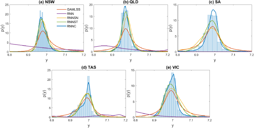
Figure 2: Out-of-sample predictive marginal calibration

Fig. 2 presents histograms of the out-of-sample observations of $Y$ for each region during the evaluation period. Also plotted are the average predictive densities $\hat{F}$ for the five forecasting methods, allowing a visual comparison of out-of-sample marginal calibration. The copula model (RNNC) produces forecasts that are most accurately calibrated, followed by RNNSN and RNNST. However, GAMLSS and RNN both exhibit poor predictive marginal calibration. The exceptionally wide intervals for RNN are caused by extremely inaccurate density forecasts at horizons close to 24 hours ahead as characterized further below.

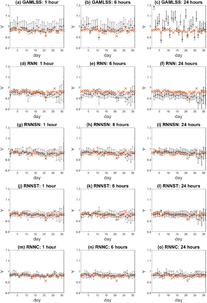
Figure 3: Prediction intervals for NSW prices at 12:00 during July 2019

To visualize the predictive densities, Fig. 3 plots the 95% prediction intervals for forecasts made during the month of July 2019. Results from the five methods for forecasts 1, 6 and 24 hours ahead are given in separate panels. RNN forecasts are negatively biased, and for some days lack “sharpness” (Gneiting et al., 2007). The latter is because a high variance is necessary to capture the price spikes in the training sample using a distribution with symmetric thin tails for the errors at (LABEL:eq:ESN). In contrast, skew-normal disturbances (RNNSN) can produce a heavier upper tail through right skew, but at the expense of overly sharp densities. De-coupling of the level of asymmetry from the kurtosis through skew-$t$ disturbances (RNNST) allows for asymmetric predictive densities with heavy tails. RNN, RNNSN and RNNST all have probabilistic forecasts that are nearly homoscedastic, because they are ensembles of homoscedastic Bayesian predictive densities. In contrast RNNC allows for a much heavier upper tail for electricity prices and heteroscedasticity; the latter is because it is a distributional model. Last, the performance of the benchmark GAMLSS model (which is also a distributional model) declines substantially over the forecast horizon.

5.3.2 Forecast accuracy

To assess forecast accuracy we compute the metrics outlined in Sec. 5.2 for each of the five methods. Table 1 reports out-of-sample point forecast accuracy, and the asymmetric deep time series models RNNSN, RNNST and RNNC are more accurate than RNN and GAMLSS in terms of MAE at all horizons, but not by the RMSE metric at short horizons. At horizons of 12 or more hours, RNNC produces the most accurate point forecasts. However, the main objective is accurate probabilistic forecasting, and Table 2 reports out-of-sample metrics for this. RNN is the poorest method by all measures, which is unsurprising given the asymmetry and heavy tails in even logarithmic prices. GAMLSS is also very poor overall. RNNST is more accurate than RNNSN, demonstrating that allowing for heavy tails increases accuracy over-and-above allowing for asymmetry. However, it is the deep copula model RNNC that provides clearly superior forecasts at all points in the forecast horizon, both in terms of the entire density (as measured using CRPS) and the upper and lower tails (as measured by the quantile scores and upper tail loss function).

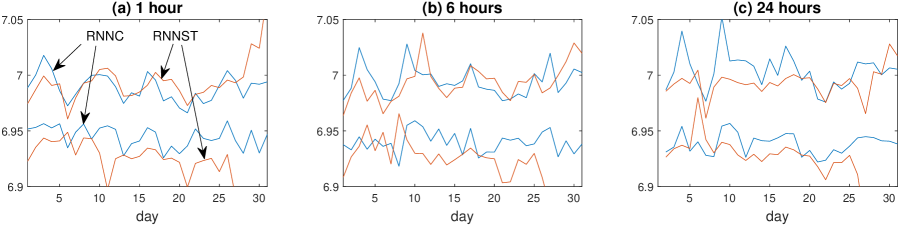
Figure 4: Tail risk for NSW prices at 12:00 during July 2019

Fig. F in the WA plots the full quantile score functions (pinball loss). The poor calibration of the RNN and GAMLSS probabilistic forecasts is clear, as is the superiority of the asymmetric deep time series models (in particular RNNC). To compare the probabilistic forecasts for the two most accurate models (RNNC and RNNST) Fig. 4 plots the expected shortfall ($E(Y|Y<F^{-1}(\alpha))$ for $\alpha=0.025$) and expected longrise ($E(Y|Y>F^{-1}(\alpha))$ for $\alpha=0.975$) at 12:00 during July 2019 for both models. The RNNC produces predictive forecasts that exhibit substantial heteroscedasticity and are sharper (i.e. lower spread between the longrise and shortfall) than the RNNST. These differences in the two deep time series models are because RNNC is a distributional time series model, whereas RNNST is not. Finally, Table 3 reports the coverage of the predictive distributions at the 95% level, and there is a substantial difference between the methods, with the predictive distributions from RNNC exhibiting superior coverage at all horizons.

6 Incorporating Probabilistic Forecasts of Demand

We now show how to extend the deep time series models to include demand forecasts as additional information in a flexible fashion, allowing for greater price forecast accuracy.

6.1 Role of demand forecasts

Demand for electricity is almost perfectly inelastic to price in the short term because individual users face fixed tariffs. As demand varies over time, the spot price traces out the average supply curve. This explains the occurrence of price “spikes” because electricity supply curves are typically kinked, and for short periods of time demand can exceed the location of this kink; see Geman and Roncoroni (2006), Clements et al. (2015), Smith and Shively (2018) and Ziel and Steinert (2016). An implication is that including accurate demand forecasts in a price forecasting model may increase its accuracy, particularly for the upper tail.

However, incorporating demand forecasts into most existing time series models for price is difficult for two reasons. First, multiple aspects of probabilistic demand forecasts beyond the point forecast are likely to increase the accuracy of probabilistic price forecasts. Second, demand forecasts are likely to be related to future prices in a highly nonlinear fashion, particularly when combined with past price values. However, both difficulties can be addressed by incorporating multiple summaries of the demand forecast distribution as additional elements of the feature vector of a deep time series model.

6.2 NSW demand forecasts

Methods for accurate short term probabilistic forecasting of demand are well established, with examples for NSW demand provided by Smith (2000) and Cottet and Smith (2003). AEMO makes demand forecasts publicly available, which are updated every half hour by an automated system. The forecasts are of the 10th, 50th (i.e. median) and 90th percentiles of demand at a half-hourly resolution over a horizon of one week. We employ demand forecasts for NSW that are exactly 24 hours ahead, to forecast NSW prices 24 hours ahead. Thus, only demand forecasts truly available at the forecast origin $T$ were used. We label the three percentile forecasts of NSW demand as $\mbox{D}10,\mbox{D}50$ and $\mbox{D}90$. Fig. D in the Web App. plots actual demand against $\mbox{D}50$ during 2019, showing the high degree of point forecast accuracy. However, empirical coverage during 2019 suggests some minor miscalibration, with 12.1%, 62.5% and 95.6% of demand observations falling below $\mbox{D}10,\mbox{D}50$ and $\mbox{D}90$, respectively.

6.3 NSW price forecasting study

The forecasting study was extended, where the NSW demand forecasts were included in the feature vectors of our two best performing deep time series models, RNNST and RNNC, for forecasting NSW price. For RNNST

$$\text{\boldmath$x$}_{t}=(1,Y_{\mbox{\tiny{NSW}},t-1},Y_{\mbox{\tiny{NSW}},t-2},\ldots,Y_{\mbox{\tiny{NSW}},t-48},Y_{\mbox{\tiny{NSW}},t-96},Y_{\mbox{\tiny{NSW}},t-144},\ldots,Y_{\mbox{\tiny{NSW}},t-336},\mbox{D}10_{t},\mbox{D}50_{t},\mbox{D}90_{t})^{\prime}\,,$$

so that $n_{x}=58$. The feature vector for RNNC contained the equivalent lagged values of the transformed series $Z_{\mbox{\tiny{NSW}},t}=\Phi_{1}^{-1}(F_{Y}(Y_{\mbox{\tiny{NSW}},t}))$, and the three demand forecasts. For comparison, the two models without the demand forecasts (so $n_{x}=55$) are also used.

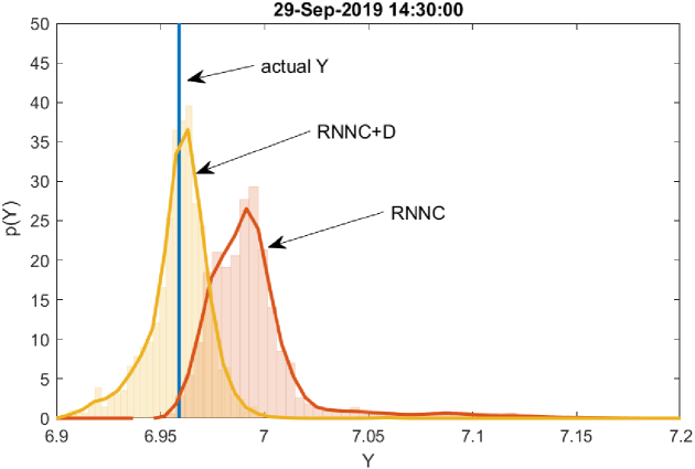
Figure 5: Density forecast of NSW price with and without demand forecast information

Table 4 reports the average value of the forecast metrics over the evaluation period. Including the demand forecasts as features decreases the accuracy of the point forecasts and the CRPS metric for both models. However, upper tail forecast accuracy increased significantly for the RNNC. This is important in this application because short periods of very high prices often dominate the profitability of participants in the NEM. To illustrate, Figure 5 plots the density forecast where the inclusion of the demand forecast information greatly increased accuracy (other examples are given in Fig. G of the WA).

Finally, we also experimented with employing the ESN at (LABEL:eq:ESN) without the quadratic term in the output layer, but found that this did decrease forecast accuracy significantly. Moreover, including ridge priors with different values of $\tau^{2}$ for the linear and quadratic terms in the output layer had little effect on forecast accuracy; see Part F of the WA for further details.

7 Conclusion

This paper makes contributions to both the time series and energy economics literatures. We propose new deep time series models that exploit the reservoir computing techniques found in ESNs for high frequency time series. Recasting a quadratic ESN as a statistical time series model, with a shrinkage prior for regularization of the output layer weights, allows for uncertainty quantification and probabilistic forecasting. Our first approach is to allow for different error distributions for the output layer, extending the Bayesian methodology of McDermott and Wikle (2017, 2019). However, our main methodological contribution is the proposal of a new deep distributional time series model. This is obtained by constructing the implicit copula of a Gaussian probabilistic ESN, and extends the deep distributional regression method of Klein et al. (2020) to time series. This copula is a deep process on the feature space, allowing for highly adaptive nonlinear serial dependence, and generalizing existing echo state Gaussian processes (Chatzis and Demiris, 2011). When combined with a nonparametric estimate of $p_{Y}$, it allows for marginal calibration. The entire density forecast is a function of the feature vector through (10), unlike with the other deep time series models. Our empirical work also suggests that accurate in-sample marginal calibration also results in more accurate calibration of both the out-of-sample marginal and predictive distributions.

While the distribution of intraday electricity prices have a sizable predictable component, these time series are complex (Ignatieva and Trück, 2016, Manner et al., 2019). Key to their accurate modeling and forecasting is to capture jointly three features: nonlinear serial dependence, high levels of asymmetry and kurtosis, and strong time-variation in the distribution. All our proposed deep time series models account for the first feature, while allowing for skew-normal or skew-$t$ disturbances also accounts for the second. However, only the deep copula model allows for all three, producing the most accurate probabilistic forecasts. Recent models (Ziel and Steinert, 2016, Shah and Lisi, 2020) suggest that including demand forecasts may further increase probabilistic forecasting accuracy. We find this to be the case for the upper tail of the 24 hour ahead NSW electricity prices when including demand forecasts as features in the deep copula model.

Last, we highlight two areas for future work. First, estimation of our deep time series models using variational methods, rather than MCMC, has the potential to speed up computations. Second, there are other applications of our deep time series models. One example is macroeconomic forecasting, where large regularized time-varying parameter models are popular (Bitto and Frühwirth-Schnatter, 2019, Carriero et al., 2019, Huber et al., 2020). The deep time series models provide a flexible alternative, as they can incorporate feature vectors of many economic variables regularized through the reservoir structure of the ESN, plus Bayesian shrinkage of the output layer coefficients. Moreover, the copula model can produce time-varying and asymmetric probabilistic forecasts, which is a feature of this problem.

Table 1: Point forecast accuracy of models during the evaluation period

	Hours Ahead in the Forecast Horizon
Model	0.5 hour	1 hour	2 hours	3 hours	6 hours	12 hours	24 hours
	MAE
GAMLSS	0.0226∗∗∗	0.0314∗∗∗	0.0408∗∗∗	0.0468∗∗∗	0.0591∗∗∗	0.0692∗∗∗	0.0766∗∗∗
RNN	0.0249∗∗∗	0.0319∗∗∗	0.0411∗∗∗	0.0494∗∗∗	0.0600∗∗∗	0.0722∗∗∗	0.0800∗∗∗
RNNSN	0.0221∗∗∗	0.0219∗	0.0239	0.0252	0.0262	0.0268∗∗	0.0278∗∗∗
RNNST	0.0189	0.0210	0.0231	0.0242	0.0250	0.0255∗∗∗	0.0257∗∗∗
RNNC	0.0169	0.0194	0.0224	0.0238	0.0252	0.0244	0.0239
	RMSE
GAMLSS	0.0340${}^{\mbox{\tiny{+}}}$	0.0461${}^{\mbox{\tiny{++}}}$	0.0610${}^{\mbox{\tiny{+++}}}$	0.0623${}^{\mbox{\tiny{+++}}}$	0.0644${}^{\mbox{\tiny{+++}}}$	0.0653	0.0661
RNN	0.0537	0.0616${}^{\mbox{\tiny{**}}}$	0.0712	0.0797	0.0935	3.7173∗∗∗	16.5496∗∗∗
RNNSN	0.0538	0.0572	0.0603	0.0615	0.0623	0.0629	0.0638
RNNST	0.0528${}^{\mbox{\tiny{+}}}$	0.0571	0.0603	0.0612	0.0623	0.0630	0.0635
RNNC	0.0538	0.0573	0.0613	0.0638	0.0657	0.0632	0.0629

Both the system-weighted mean absolute error (MAE) and root mean squared error (RMSE) are reported. Results are given for the four deep time series models, plus GAMLSS. Results of a two-sided Diebold-Mariano test of the equality of the mean error of the RNNC with each of the other models are reported. Rejection of the null hypothesis of equal means at the 10%, 5% and 1% levels are denoted by “*”, “**” and “***” if favorable to the RNNC model, or by “+”, “++” and “+++” if unfavorable.

Table 2: Probabilistic forecast accuracy during the evaluation period.

	Hours Ahead in the Forecast Horizon
Model	0.5 hour	1 hour	2 hours	3 hours	6 hours	12 hours	24 hours
	CRPS
GAMLSS	0.0180∗∗∗	0.0252∗∗∗	0.0335∗∗∗	0.0392∗∗∗	0.0508∗∗∗	0.0601∗∗∗	0.0652∗∗∗
RNN	0.0203∗∗∗	0.0235∗∗∗	0.0299∗∗∗	0.0364∗∗∗	0.0449∗∗∗	0.0574∗∗∗	0.4061∗∗∗
RNNSN	0.0174∗∗∗	0.0177∗∗	0.0191	0.0201	0.0207	0.0212∗∗	0.0219∗∗∗
RNNST	0.0157∗∗∗	0.0172∗∗∗	0.0187∗∗∗	0.0195	0.0201	0.0206∗∗∗	0.0208∗∗∗
RNNC	0.0135	0.0154	0.0177	0.0189	0.0199	0.0193	0.0187
	Joint Upper Tail Loss at $\alpha=0.975$
GAMLSS	31.6394∗	32.4717∗∗∗	33.2367∗∗∗	33.9396∗∗∗	35.9352∗∗∗	40.0541∗∗∗	39.7960∗∗∗
RNN	30.8568	31.5025	33.3171	35.5605	39.2732∗∗	41.9374∗∗∗	33.4037∗∗∗
RNNSN	32.1052∗∗	31.2797	31.6342	31.6492	31.7099	31.5852∗∗∗	31.3780∗∗∗
RNNST	31.3493∗	31.4414	31.6911	32.0056∗	31.8607	32.2372∗∗∗	31.8694∗∗∗
RNNC	30.1002	30.6244	31.0090	31.0934	31.1121	30.6238	29.7661
	Quantile Score at $\alpha=0.95$
GAMLSS	0.0056∗∗∗	0.0069∗∗∗	0.0082∗∗∗	0.0093∗∗∗	0.0124∗∗∗	0.0190∗∗∗	0.0198∗∗∗
RNN	0.0050	0.0057	0.0078∗∗∗	0.0107∗∗∗	0.0155∗∗∗	0.0201∗∗∗	1.0808∗∗∗
RNNSN	0.0056	0.0050	0.0054	0.0055	0.0057	0.0058∗	0.0060∗∗∗
RNNST	0.0048	0.0050	0.0054	0.0057∗∗	0.0057∗	0.0062∗∗∗	0.0063∗∗∗
RNNC	0.0036	0.0043	0.0048	0.0050	0.0052	0.0050	0.0046
	Quantile Score at $\alpha=0.05$
GAMLSS	0.0049∗∗∗	0.0080∗∗∗	0.0129∗∗∗	0.0167∗∗∗	0.0242∗∗∗	0.0260∗∗∗	0.0298∗∗∗
RNN	0.0047	0.0053	0.0057∗∗∗	0.0061	0.0069∗∗∗	0.0096∗∗∗	0.5602∗∗∗
RNNSN	0.0046∗∗	0.0055	0.0056	0.0062	0.0061	0.0064	0.0065
RNNST	0.0048∗∗∗	0.0055∗	0.0059∗∗	0.0061	0.0064	0.0063	0.0066
RNNC	0.0039	0.0046	0.0053	0.0058	0.0061	0.0059	0.0057

System-weighted metrics are reported for the four deep time series models, plus GAMLSS, at different points in time during a 24 hour forecast horizon. Lower values suggest greater accuracy. Results of a two-sided Diebold-Mariano test of the equality of the mean error of the RNNC with each of the other models are reported. Rejection of the null hypothesis of equal means at the 10%, 5% and 1% levels are denoted by “*”, “**” and “***” if favorable to the RNNC model, or by “+”, “++” and “+++” if unfavorable.

Table 3: Coverage of 95% prediction intervals during the evaluation period.

	Hours Ahead in the Forecast Horizon
Model	0.5 hour	1 hour	2 hours	3 hours	6 hours	12 hours	24 hours
GAMLSS	0.9078	0.8148	0.7278	0.6928	0.6476	0.5838	0.5208
RNN	0.8715	0.8609	0.7906	0.7173	0.6336	0.5698	0.6124
RNNSN	0.8496	0.8386	0.8354	0.8187	0.8123	0.7998	0.7759
RNNST	0.8550	0.8424	0.8353	0.8216	0.8171	0.7955	0.7667
RNNC	0.9279	0.9012	0.8791	0.8741	0.8620	0.8594	0.8706

Results are reported for the four deep time series models, plus GAMLSS, at different points in time in the 24 hour forecast horizon. Values closer to 0.95 indicate improved calibration of the probabilistic forecasts.

Table 4: NSW price forecast accuracy when including demand forecast information.

Model	MAE	RMSE	CRPS		JS	QS95	QS05	C95
	Point and Density Accuracy				Tail Accuracy
RNNC+D	0.0192	0.0314	0.0146		30.6902	0.0045	0.0025	82.6%
RNNC	0.0188${}^{\mbox{\tiny{+++}}}$	0.0311${}^{\mbox{\tiny{+++}}}$	0.0144${}^{\mbox{\tiny{+++}}}$		31.0350∗∗	0.0048∗∗∗	0.0023	84.5%
RNNST	0.0250∗∗∗	0.0401	0.0221∗∗∗		39.4411∗∗∗	0.0121∗∗∗	0.0049∗∗∗	46.2 %
RNNST+D	0.0256∗∗∗	0.0395	0.0222∗∗∗		39.6431∗∗∗	0.0123∗∗∗	0.0046∗∗∗	53.9%

Accuracy of 24 hour ahead NSW (logarithmic) price forecasts during the evaluation period. Models that include 24 hour ahead demand forecast information as features are labelled as “+D”. The metrics are described in the text, and include the joint score (JS) at $\alpha=0.975$, quantile score (QS) at $\alpha=0.95,0.05$, and the empirical coverage of the 95% prediction intervals (C95). Results of a two-sided Diebold-Mariano test of the equality of the mean error of the RNNC+D with the other methods are reported. Rejection of the null hypothesis of equal means at the 10%, 5% and 1% levels are denoted by “*”, “**” and “***” if favorable to the RNNC+D model, or by “+”, “++” and “+++” if unfavorable.

Boxplots are of $Y=\log(\mbox{PRICE}+1001)$ for each hour of the day during the period 1 January 2019 to 31 December 2019.

Histograms are of the out-of-sample observations of $Y$ during the evaluation period (1 May - 31 December 2019). The average predictive density for each method is given for the four deep time series models, plus the GAMLSS benchmark. The deep time series copula model (RNNC) produces average densities close to the bounded KDEs fit to the in-sample data found in Fig. B of the WA by construction. The panels correspond to forecast prices in (a) NSW, (b) QLD, (c) SA, (d) TAS and (e) VIC.

Panels correspond to forecasts from the five methods made 1, 6 and 24 hours ahead. In each panel, 95% prediction intervals are denoted by a vertical bar, with the predictive mean given by a grey cross. The true values are denoted with a red cross. Results are presented on the logarithmic scale for clarity.

Panels (a)-(c) correspond to forecasts made 1, 6 and 24 hours ahead for the RNNC (in blue) and RNNST (in red). In each panel, both the the expected longrise $E(Y|Y>Q(\alpha))$ at $\alpha=0.975$ and the expected shortfall $E(Y|Y<Q(\alpha))$ at $\alpha=0.025$ are plotted. Results are presented on the logarithmic scale for clarity.

Density forecast of NSW electricity price for 29-Sep-2019 at 14:30, where the inclusion of demand forecast information greatly improved accuracy (as measured by CRPS). The density forecast without demand forecast information is labelled as “RNNC”, and with as “RNNC+D”. The actual price is marked with a blue vertical line.

References

- Amjady (2006) Amjady, N. (2006). Day-ahead price forecasting of electricity markets by a new fuzzy neural network. IEEE Transactions on Power Systems, 21(2):887–896.
- Apergis et al. (2019) Apergis, N., Gozgor, G., Lau, C. K. M., and Wang, S. (2019). Decoding the Australian electricity market: New evidence from three-regime hidden semi-Markov model. Energy Economics, 78:129–142.
- Australian Energy Regulator (2019) Australian Energy Regulator (2019). State of the energy market report: data update.
- Azzalini and Capitanio (2003) Azzalini, A. and Capitanio, A. (2003). Distributions generated by perturbation of symmetry with emphasis on a multivariate skew t-distribution. Journal of the Royal Statistical Society: Series B, 65(2):367–389.
- Bianchi et al. (2020) Bianchi, D., Büchner, M., and Tamoni, A. (2020). Bond risk premiums with machine learning. The Review of Financial Studies, Forthcoming.
- Bitto and Frühwirth-Schnatter (2019) Bitto, A. and Frühwirth-Schnatter, S. (2019). Achieving shrinkage in a time-varying parameter model framework. Journal of Econometrics, 210(1):75–97.
- Bunn et al. (2016) Bunn, D., Andresen, A., Chen, D., and Westgaard, S. (2016). Analysis and forecasting of electricty price risks with quantile factor models. The Energy Journal, 37(1).
- Carriero et al. (2019) Carriero, A., Clark, T. E., and Marcellino, M. (2019). Large Bayesian vector autoregressions with stochastic volatility and non-conjugate priors. Journal of Econometrics, 212(1):137–154.
- Chatzis and Demiris (2011) Chatzis, S. P. and Demiris, Y. (2011). Echo state Gaussian process. IEEE Transactions on Neural Networks, 22(9):1435–1445.
- Christensen et al. (2012) Christensen, T. M., Hurn, A. S., and Lindsay, K. A. (2012). Forecasting spikes in electricity prices. International Journal of Forecasting, 28(2):400–411.
- Clements et al. (2015) Clements, A., Herrera, R., and Hurn, A. (2015). Modelling interregional links in electricity price spikes. Energy Economics, 51:383–393.
- Cottet and Smith (2003) Cottet, R. and Smith, M. (2003). Bayesian modeling and forecasting of intraday electricity load. Journal of the American Statistical Association, 98(464):839–849.
- Feng et al. (2018) Feng, G., He, J., and Polson, N. G. (2018). Deep learning for predicting asset returns. arXiv preprint arxiv:1804.09314.
- Fissler et al. (2016) Fissler, T., Ziegel, J. F., et al. (2016). Higher order elicitability and Osband’s principle. The Annals of Statistics, 44(4):1680–1707.
- Frühwirth-Schnatter and Pyne (2010) Frühwirth-Schnatter, S. and Pyne, S. (2010). Bayesian inference for finite mixtures of univariate and multivariate skew-normal and skew-t distributions. Biostatistics, 11(2):317–336.
- Geman and Roncoroni (2006) Geman, H. and Roncoroni, A. (2006). Understanding the fine structure of electricity prices. The Journal of Business, 79(3):1225–1261.
- Gianfreda and Bunn (2018) Gianfreda, A. and Bunn, D. (2018). A stochastic latent moment model for electricity price formation. Operations Research, 66(5):1189–1203.
- Gneiting (2011) Gneiting, T. (2011). Quantiles as optimal point forecasts. International Journal of forecasting, 27(2):197–207.
- Gneiting et al. (2007) Gneiting, T., Balabdaoui, F., and Raftery, A. E. (2007). Probabilistic forecasts, calibration and sharpness. Journal of the Royal Statistical Society Series B, 69(2):243–268.
- Gneiting and Katzfuss (2014) Gneiting, T. and Katzfuss, M. (2014). Probabilistic forecasting. Annual Review of Statistics and Its Application, 1:125–151.
- Goodfellow et al. (2016) Goodfellow, I., Bengio, Y., and Courville, A. (2016). Deep Learning. MIT Press. http://www.deeplearningbook.org.
- Gu et al. (2020a) Gu, S., Kelly, B., and Xiu, D. (2020a). Autoencoder asset pricing models. Journal of Econometrics, Forthcoming.
- Gu et al. (2020b) Gu, S., Kelly, B., and Xiu, D. (2020b). Empirical asset pricing via machine learning. The Review of Financial Studies, Forthcoming.
- Han et al. (2020) Han, L., Kordzakhia, N., and Trück, S. (2020). Volatility spillovers in Australian electricity markets. Energy Economics, page Forthcoming.
- Higgs (2009) Higgs, H. (2009). Modelling price and volatility inter-relationships in the Australian wholesale spot electricity markets. Energy Economics, 31(5):748–756.
- Huber et al. (2020) Huber, F., Koop, G., and Onorante, L. (2020). Inducing sparsity and shrinkage in time-varying parameter models. Journal of Business and Economic Statistics, pages 1–15.
- Huurman et al. (2012) Huurman, C., Ravazzolo, F., and Zhou, C. (2012). The power of weather. Computational Statistics & Data Analysis, 56(11):3793–3807.
- Ignatieva and Trück (2016) Ignatieva, K. and Trück, S. (2016). Modeling spot price dependence in Australian electricity markets with applications to risk management. Computers & Operations Research, 66:415–433.
- Jaeger (2007) Jaeger, H. (2007). Echo state network. Scholarpedia, 2(9):2330.
- Janczura and Weron (2010) Janczura, J. and Weron, R. (2010). An empirical comparison of alternate regime-switching models for electricity spot prices. Energy economics, 32(5):1059–1073.
- Karakatsani and Bunn (2008) Karakatsani, N. V. and Bunn, D. W. (2008). Intra-day and regime-switching dynamics in electricity price formation. Energy Economics, 30(4):1776–1797.
- Kirschen and Strbac (2018) Kirschen, D. S. and Strbac, G. (2018). Fundamentals of Power System Economics. John Wiley & Sons.
- Klein and Kneib (2016) Klein, N. and Kneib, T. (2016). Scale-dependent priors for variance parameters in structured additive distributional regression. Bayesian Analysis, 11(4):1071–1106.
- Klein et al. (2020) Klein, N., Nott, D. J., and Smith, M. S. (2020). Marginally calibrated deep distributional regression. Journal of Computational and Graphical Statistics, Forthcoming.
- Knittel and Roberts (2005) Knittel, C. R. and Roberts, M. R. (2005). An empirical examination of restructured electricity prices. Energy Economics, 27(5):791–817.
- Lago et al. (2018) Lago, J., De Ridder, F., and De Schutter, B. (2018). Forecasting spot electricity prices: Deep learning approaches and empirical comparison of traditional algorithms. Applied Energy, 221:386–405.
- Lukoševičius and Jaeger (2009) Lukoševičius, M. and Jaeger, H. (2009). Reservoir computing approaches to recurrent neural network training. Computer Science Review, 3(3):127–149.
- Mandal et al. (2007) Mandal, P., Senjyu, T., Urasaki, N., Funabashi, T., and Srivastava, A. K. (2007). A novel approach to forecast electricity price for PJM using neural network and similar days method. IEEE Transactions on Power Systems, 22(4):2058–2065.
- Manner et al. (2019) Manner, H., Fard, F. A., Pourkhanali, A., and Tafakori, L. (2019). Forecasting the joint distribution of Australian electricity prices using dynamic vine copulae. Energy Economics, 78:143–164.
- Manner et al. (2016) Manner, H., Türk, D., and Eichler, M. (2016). Modeling and forecasting multivariate electricity price spikes. Energy Economics, 60:255–265.
- McDermott and Wikle (2017) McDermott, P. L. and Wikle, C. K. (2017). An ensemble quadratic echo state network for non-linear spatio-temporal forecasting. Stat, 6(1):315–330.
- McDermott and Wikle (2019) McDermott, P. L. and Wikle, C. K. (2019). Deep echo state networks with uncertainty quantification for spatio-temporal forecasting. Environmetrics, 30(3):e2553.
- Misiorek et al. (2006) Misiorek, A., Trueck, S., and Weron, R. (2006). Point and interval forecasting of spot electricity prices: Linear vs. non-linear time series models. Studies in Nonlinear Dynamics & Econometrics, 10(3).
- Narajewski and Ziel (2020) Narajewski, M. and Ziel, F. (2020). Ensemble forecasting for intraday electricity prices: Simulating trajectories. Applied Energy, Forthcoming.
- Nelsen (2006) Nelsen, R. B. (2006). An Introduction to Copulas. Springer-Verlag, New York, Secaucus, NJ, USA.
- Nolde et al. (2017) Nolde, N., Ziegel, J. F., et al. (2017). Elicitability and backtesting: Perspectives for banking regulation. The Annals of Applied Statistics, 11(4):1833–1874.
- Nowotarski et al. (2013) Nowotarski, J., Tomczyk, J., and Weron, R. (2013). Robust estimation and forecasting of the long-term seasonal component of electricity spot prices. Energy Economics, 39:13–27.
- Nowotarski and Weron (2018) Nowotarski, J. and Weron, R. (2018). Recent advances in electricity price forecasting: A review of probabilistic forecasting. Renewable and Sustainable Energy Reviews, 81:1548–1568.
- Panagiotelis and Smith (2008) Panagiotelis, A. and Smith, M. (2008). Bayesian density forecasting of intraday electricity prices using multivariate skew t distributions. International Journal of Forecasting, 24(4):710–727.
- Pascanu et al. (2013) Pascanu, R., Mikolov, T., and Bengio, Y. (2013). On the difficulty of training recurrent neural networks. In Proceedings of the 30th International Conference on International Conference on Machine Learning - Volume 28, ICML’13, pages III–1310–III–1318.
- Pircalabu and Benth (2017) Pircalabu, A. and Benth, F. E. (2017). A regime-switching copula approach to modeling day-ahead prices in coupled electricity markets. Energy Economics, 68:283–302.
- Rafiei et al. (2016) Rafiei, M., Niknam, T., and Khooban, M.-H. (2016). Probabilistic forecasting of hourly electricity price by generalization of elm for usage in improved wavelet neural network. IEEE Transactions on Industrial Informatics, 13(1):71–79.
- Raiffa and Schleifer (1961) Raiffa, H. and Schleifer, R. (1961). Applied statistical decision theory. Division of Research, Graduate School of Business Administration, Harvard University.
- Rigby and Stasinopoulos (2005) Rigby, R. A. and Stasinopoulos, D. M. (2005). Generalized additive models for location, scale and shape. Journal of the Royal Statistical Society Series C, 54(3):507–554.
- Serinaldi (2011) Serinaldi, F. (2011). Distributional modeling and short-term forecasting of electricity prices by generalized additive models for location, scale and shape. Energy Economics, 33(6):1216–1226.
- Shah and Lisi (2020) Shah, I. and Lisi, F. (2020). Forecasting of electricity price through a functional prediction of sale and purchase curves. Journal of Forecasting, 39(2):242–259.
- Smith (2000) Smith, M. (2000). Modeling and short-term forecasting of New South Wales electricity system load. Journal of Business & Economic Statistics, 18(4):465–478.
- Smith et al. (2012) Smith, M. S., Gan, Q., and Kohn, R. J. (2012). Modelling dependence using skew t copulas: Bayesian inference and applications. Journal of Applied Econometrics, 27(3):500–522.
- Smith and Shively (2018) Smith, M. S. and Shively, T. S. (2018). Econometric modeling of regional electricity spot prices in the Australian market. Energy Economics, 74:886–903.
- Ugurlu et al. (2018) Ugurlu, U., Oksuz, I., and Tas, O. (2018). Electricity price forecasting using recurrent neural networks. Energies, 11(5):1255.
- Weron (2014) Weron, R. (2014). Electricity price forecasting: A review of the state-of-the-art with a look into the future. International Journal of Forecasting, 30(4):1030–1081.
- Wilson and Ghahramani (2010) Wilson, A. G. and Ghahramani, Z. (2010). Copula processes. In Advances in Neural Information Processing Systems, pages 2460–2468.
- Ziel and Steinert (2016) Ziel, F. and Steinert, R. (2016). Electricity price forecasting using sale and purchase curves: The X-Model. Energy Economics, 59:435–454.