Projection Efficient Subgradient Method and Optimal Nonsmooth Frank-Wolfe Method

Abstract

We consider the classical setting of optimizing a nonsmooth Lipschitz continuous convex function over a convex constraint set, when having access to a (stochastic) first-order oracle (FO) for the function and a projection oracle (PO) for the constraint set. It is well known that to achieve $\varepsilon$-suboptimality in high-dimensions, $\Theta(\varepsilon^{-2})$ FO calls are necessary [64]. This is achieved by the projected subgradient method (PGD) [11]. However, PGD also entails ${\mathcal{O}}(\varepsilon^{-2})$ PO calls, which may be computationally costlier than FO calls (e.g. nuclear norm constraints). Improving this PO calls complexity of PGD is largely unexplored, despite the fundamental nature of this problem and extensive literature. We present first such improvement. This only requires a mild assumption that the objective function, when extended to a slightly larger neighborhood of the constraint set, still remains Lipschitz and accessible via FO. In particular, we introduce MOPES method, which carefully combines Moreau-Yosida smoothing and accelerated first-order schemes. This is guaranteed to find a feasible $\varepsilon$-suboptimal solution using only ${\mathcal{O}}(\varepsilon^{-1})$ PO calls and optimal ${\mathcal{O}}(\varepsilon^{-2})$ FO calls. Further, instead of a PO if we only have a linear minimization oracle (LMO, à la Frank-Wolfe) to access the constraint set, an extension of our method, MOLES, finds a feasible $\varepsilon$-suboptimal solution using ${\mathcal{O}}(\varepsilon^{-2})$ LMO calls and FO calls—both match known lower bounds [54], resolving a question left open since [84]. Our experiments confirm that these methods achieve significant speedups over the state-of-the-art, for a problem with costly PO and LMO calls.

1 Introduction

In this paper, we consider the nonsmooth convex optimization (NSCO) problem with the First-order Oracle (FO) and the Projection Oracle (PO) defined as:

$$\text{NSCO}:\min_{x}\ f(x),\ \text{s.t.}\ x\in\mathcal{X}\ ,\ \ \text{FO}(x)\in\partial f(x),\ \text{and }\text{PO}(x)=\mathcal{P}_{\mathcal{X}}(x)=\mathop{\mathrm{argmin}}_{y\in\mathcal{X}}\|y-x\|_{2}^{2},$$ (1)

where $f:\mathbb{R}^{d}\rightarrow\mathbb{R}$ is a convex Lipschitz-continuous function, and $\mathcal{X}\subseteq\mathbb{R}^{d}$ is a convex constraint. When queried at a point $x$, FO returns a subgradient of $f$ at $x$ and PO returns the projection of $x$ onto $\mathcal{X}$. NSCO is a fundamental problem with a long history and several important applications including support vector machines (SVM) [12], robust learning [44], and utility maximization in finance [82].

Finding an $\varepsilon$-suboptimal solution for this problem requires $\Omega(\varepsilon^{-2})$ FO calls in the worst case, when the dimension $d$ is large [64]. This lower bound is tightly matched by the projected subgradient method (PGD). Unfortunately, PGD also uses one PO call after every FO call, resulting in a PO calls complexity (PO-CC)—the number of times PO needs to be invoked—of ${\Theta}(\varepsilon^{-2})$. This can be a major bottleneck in solving several practical problems like collaborative filtering [79], where the cost of a PO is often higher than the cost of an FO call. This begs the natural question, which surprisingly is largely unexplored in the general nonsmooth optimization setting: Can we design an algorithm whose PO calls complexity is significantly better than the optimal FO calls complexity $O(\varepsilon^{-2})$?

	Randomized Smoothing	State-of-the-art	Our results	Lower
	dimension dependent	dimension-free	(Theorems 1 and2)	bound
SFO	${\mathcal{O}}((G^{2}+\sigma^{2})/\varepsilon^{2})$ [27]	${\mathcal{O}}((G^{2}+\sigma^{2})/\varepsilon^{2})$ [65]	$\boldsymbol{{\mathcal{O}}((G^{2}+\sigma^{2})/\varepsilon^{2})}$	$\Omega((G^{2}+\sigma^{2})/\varepsilon^{2})$ [64]
PO	${\mathcal{O}}(d^{1/4}G/\varepsilon)$ [27]	${\mathcal{O}}(G^{2}/\varepsilon^{2})^{\star}$ [65]	$\boldsymbol{{\mathcal{O}}(G/\varepsilon)}$	Open problem
SFO	${\mathcal{O}}(\sqrt{d}\,(G^{2}+\sigma^{2})^{2}/\varepsilon^{4})$ [54]	${\mathcal{O}}((G^{2}+\sigma^{2})/\varepsilon^{2})^{\dagger}$	$\boldsymbol{{\mathcal{O}}((G^{2}+\sigma^{2})/\varepsilon^{2})}$	$\Omega((G^{2}+\sigma^{2})/\varepsilon^{2})$ [64]
LMO	${\mathcal{O}}(\sqrt{d}\,G^{2}/\varepsilon^{2})$ [54]	${\mathcal{O}}((G^{2}+\sigma^{2})^{2}/\varepsilon^{4})^{\dagger}$	$\boldsymbol{{\mathcal{O}}(G^{2}/\varepsilon^{2})}$	$\Omega(G^{2}/\varepsilon^{2})$ [54]

Table 1: Comparison of SFO (3), PO (1) & LMO (2) calls complexities of our methods and state-of-the-art algorithms, and corresponding lower-bounds for finding an approximate minimizer of a $d$-dimensional NSCO problem (1). We assume that $f$ is convex and $G$-Lipschitz continuous, and is accessed through a stochastic subgradient oracle with a variance of $\sigma^{2}$. ^⋆requires using a minibatch of appropriate size, ^†approximates projections of PGD with FW method (FW-PGD, see Appendix B.2).

In this work, we answer the above question in the affirmative. Our first key contribution is MOreau Projection Efficient Subgradient method (MOPES), that obtains an $\varepsilon$-suboptimal solution using only ${\mathcal{O}}(\varepsilon^{-1})$ PO calls, while still ensuring that the FO calls complexity (FO-CC)—the number of times FO needs to be invoked—is optimal, i.e., ${\mathcal{O}}(\varepsilon^{-2})$. This requires a mild assumption that the function $f$ extends to a slightly larger neighborhood of the constraint set $\mathcal{X}$. Concretely, we assume that $f$ is Lipschitz continuous in this neighborhood and FO can be queried at points in this neighborhood. To the best of our knowledge, our result is the first improvement over the ${\mathcal{O}}({\varepsilon^{-2}})$ PO calls of PGD for minimizing a general nonsmooth Lipschitz continuous convex function.

We achieve this by carefully combining Moreau-Yosida regularization with accelerated first-order methods [62, 81]. As accelerated methods cannot be directly applied to a nonsmooth $f$, we can instead apply them to minimize its Moreau envelope, which is smooth (as long as $f$ is Lipschitz continuous). Although this idea has been explored, for example, in [25, 9], PO-CC has remained ${\mathcal{O}}({\varepsilon^{-2}})$, unless a much stronger and unrealistic oracle is assumed [9] with a direct access to the gradient of Moreau envelope. The key idea in breaking this barrier is to separate out the dependence on FO calls of $f$ from PO calls to $\mathcal{X}$ by: ($a$) using Moreau-Yosida regularization to split the original problem into a composite problem, where one component consists of an unconstrained optimization of the function $f$ and the other consists of a simple constrained optimization over the set $\mathcal{X}$; and ($b$) applying the gradient sliding algorithm [55] on this joint problem to ensure the above mentioned bounds for both FO and PO calls. We note that our results are limited to the Euclidean norm, since our results crucially depend on smoothness of the Moreau envelope and its regularizer, which is not known for Moreau envelopes based on general Bregman divergences [7].

In some high-dimensional problems, even a single call to the PO can be computationally prohibitive. A popular alternative, pioneered by Frank and Wolfe [28], is to replace PO by a more efficient Linear Minimization Oracle (LMO), which returns a minimizer of any linear functional $\left\langle g,\cdot\right\rangle$ over the set $\mathcal{X}$.

$$\text{LMO}\left(g\right)\in\mathop{\mathrm{argmin}}_{s\in\mathcal{X}}\left\langle g,s\right\rangle$$ (2)

Linear minimization is much faster than projection in several practical ML applications such as a nuclear norm ball constrained problems [15], video-narration alignment [1], structured SVM [51], and multiple sequence alignment and motif discovery [89]. LMO based methods have an important additional benefit of producing solutions that preserve desired structures such as sparsity and low rank. For smooth $f$, there is a long history of conditional gradient (Frank-Wolfe) methods that use ${\mathcal{O}}(\varepsilon^{-1})$ LMO calls and ${\mathcal{O}}(\varepsilon^{-1})$ FO calls to achieve $\varepsilon$-suboptimality, which achieve optimal LMO-CC [45]. For nonsmooth functions, starting from the work of [84], several approaches have been proposed, some under more assumptions. The best known upper bound on LMO calls is ${\mathcal{O}}(\sqrt{d}\varepsilon^{-2})$ which is achieved at the expense of significantly larger ${\mathcal{O}}(\varepsilon^{-4})$ FO calls. Details of these are in Section 1.1.

Our second key contribution is the algorithm MOLES, which obtains an $\varepsilon$-suboptimal solution using the optimal ${\mathcal{O}}({\varepsilon^{-2}})$ LMO and FO calls, without any additional dimension dependence. We achieve this result by extending MOPES to work with approximate projections and using the classical Frank-Wolfe (FW) method [28] to implement these approximate projections using LMO calls.

Finally, both of our methods extend naturally to the Stochastic First-order Oracle (SFO) setting, where we have access only to stochastic versions of the function’s subgradients. Stochastic versions of MOPES and MOLES still achieve the the same PO/LMO calls complexities as deterministic counterparts, while the SFO calls complexity (SFO-CC) is ${\mathcal{O}}\left((1+\sigma^{2})\epsilon^{-2}\right)$, where $\sigma^{2}$ is the variance in SFO. This again matches information theoretic lower bounds [64].

Contributions: We summarize our contributions below and in Table 1. We assume that the function $f$ extends to a slightly larger neighborhood of the constraint set $\mathcal{X}$ i.e., $f$ continues to be Lipschitz continuous and (S)FO can be queried in this neighborhood.

• We introduce MOPES and show that it is guaranteed to find an $\varepsilon$-suboptimal solution for any constrained nonsmooth convex optimization problem using ${\mathcal{O}}({\varepsilon^{-1}})$ PO calls and optimal ${\mathcal{O}}({\varepsilon^{-2}})$ SFO calls. To the best of our knowledge, for the general problem, this achieves the first improvement over ${\mathcal{O}}({\varepsilon^{-2}})$ PO-CC and SFO-CC of stochastic projected subgradient method (PGD).

• For LMO setting, we extend our method to design MOLES, that achieves the optimal SFO-CC and LMO-CC of ${\mathcal{O}}({\varepsilon^{-2}})$, and improves over the best known LMO-CC by $\sqrt{d}$.

• We also empirically evaluate MOPES and MOLES on the popular nuclear norm constrained Matrix SVM problem [85], where they achieve significant speedups over their corresponding baselines.

• Our main technical novelty is the use Moreau-Yosida regularization to separate out the constraint (PO/LMO) and function (SFO) accesses into two parts of a composite optimization problem. This enables a better control of how many times each of these oracles are accessed. This idea might be of independent interest, whenever a trade-off between PO-CC/LMO-CC and SFO-CC is desirable.

1.1 Related Work

Nonsmooth convex optimization: Nonsmooth convex optimization has been the focal point of several research works for past few decades. [64] provided information theoretic lower bound of FO calls $O(\varepsilon^{-2})$ to obtain $\varepsilon$-suboptimal solution, for the general problem. This bound is matched by the PGD method introduced independently by [34] and [59], which also implies a PO-CC of $O(\varepsilon^{-2})$. Recently, several faster PGD style methods [50, 78, 87, 48] have been proposed that exploit more structure in the given optimization function, e.g., when the function is a sum of a smooth and a nonsmooth function for which a proximal operator is available [8]. But, to the best of our knowledge, such works do not explicitly address PO-CC and are mainly concerned about optimizing FO-CC. Thus, for the worst case nonsmooth functions, these methods still suffer from $O(\varepsilon^{-2})$ PO-CC.

Smoothed surrogates: Smoothing of the nonsmooth function is another common approach in solving them [62, 66]. In particular, randomized smoothing [27, 9] techniques have been successful in bringing down FO-CC w.r.t. $\varepsilon$ but such improvements come at the cost of dimension factors. For example, [27, Corollary 2.4] provides a randomized smoothing method that has $O(d^{1/4}/\varepsilon)$ PO-CC and $O(\varepsilon^{-2})$ FO-CC. Our MOPES method guarantees significantly better PO-CC than PGD that is still independent of dimension.

One or $\log({1}/{\epsilon})$ projection methods: Starting with the work of [61], several recent works [91, 17, 88] have proposed methods that require only one or $\log({1}/{\epsilon})$ projections, under a variety of conditions on the optimization function like smoothness and strong convexity. However, these methods require that the constraint set can be written as $c(x)\leq 0$ and they require access to $\nabla c(x)$—the gradient of $c$–in each iteration. Hence, for the general nonsmooth functions, they will require at least $O(\varepsilon^{-2})$ accesses to gradients of the set’s functional form. On the other hand, our method is required to access the set at only $O(\varepsilon^{-1})$ points. Furthermore, for several practical problems, the computational complexities of computing $\nabla c(x)$ and projecting are similar. For example, when $c(x)=\|x\|_{\rm nuc}-r$ where $\|\cdot\|_{\rm nuc}$ denotes the nuclear norm (see Section 4), then both gradient of $c(x)$ as well as PO requires computation of a full-SVD of $x$.

Frank-Wolfe methods: FW or conditional gradient method [28, 59] for smooth convex optimization, which uses LMO, has found renewed interest in machine learning [92, 45] due to the efficiency of computing LMO over PO [33], and its ability to ensure atomic structure and provide coreset guarantees [22]. Over the last decade, several variants of FW method and their analyses have been proposed [54, 29, 3, 31, 58, 68, 14], and FW has been extended to stochastic nonconvex [49, 39, 75, 76, 5, 37] and online [38, 30, 52, 18, 86, 40] settings. However these methods provide dimension-free LMO-CC and SFO-CC only for smooth functions, and further it is known that FW fails to converge if subgradients are used instead of gradients [68].

Nonsmooth Frank-Wolfe methods: [84] posed an interesting question in the domain of nonsmooth optimization with LMO: can LMO-CC be reduced from the ${\mathcal{O}}(\varepsilon^{-4})$ bound (achieved by PGD with PO implemented via LMO: FW-PGD, see Appendix B.2) without increasing FO-CC significantly. On the lower bound side, [54] showed that ${\mathcal{O}}(\varepsilon^{-2})$ LMO calls are necessary. On algorithmic side, several randomized smoothing approaches combined with Frank-Wolfe methods were proposed, and can reduce LMO-CC to ${\mathcal{O}}(d^{1/2}\varepsilon^{-2})$. But, they come at the expense of increased ${\mathcal{O}}(d^{1/2}\varepsilon^{-4})$ FO calls [54, improving Theorem 5]. If we allow stronger oracles or additional structure in the problem, the complexity can be significantly improved. Assuming a stronger than LMO oracle introduced in [84], [73] shows that ${\mathcal{O}}(1/\varepsilon^{2})$ LMO-CC and FO-CC are achievable for a special class of problems with low curvatures. Another popular setting is when the nonsmooth problem admits a smooth convex-concave saddle point reformulation [35, 23, 72, 36, 41, 42, 32, 60]. Among these the best complexity is achieved by semi-proximal mirror-prox [41] which uses ${\mathcal{O}}(\varepsilon^{-2})$ LMO and ${\mathcal{O}}(\varepsilon^{-1})$ FO calls. However, for the general nonsmooth convex optimization problem with LMO, the problem posed by [84] remained open, and is resolved by our MOLES method that achieves the optimal ${\mathcal{O}}(\varepsilon^{-2})$ LMO-CC and FO-CC.

2 Preliminaries and Notations

We consider Nonsmooth Convex Optimization with FO and PO (1) or LMO (2) accesses. Let $\mathcal{X}\subset{\mathbb{R}^{d}}$ be a closed convex set of diameter $D_{\mathcal{X}}\mathrel{\mathop{:}}=\max_{x_{1},x_{1}\in\mathcal{X}}\|x_{1}-x_{2}\|$, where $\|\cdot\|$ is the Euclidean norm which corresponds to the inner product $\left\langle\cdot,\cdot\right\rangle$. Let $\mathcal{X}$ be enclosed in a closed convex set $\mathcal{X}^{\prime}\subseteq{\mathbb{R}^{d}}$ to which it is easy to project, i.e. $\mathcal{X}\subset\mathcal{X}^{\prime}$. For simplicity, let $\mathcal{X}^{\prime}$ be a Euclidean ball of radius $R\leq D_{\mathcal{X}}$ around origin. We can satisfy $R=D_{\mathcal{X}}$ by re-centering ${\mathbb{R}^{d}}$ around any feasible point of $\mathcal{X}$. We assume $f:\mathcal{X}^{\prime}\to\mathbb{R}$ to be a proper, lower semi-continuous (l.s.c.), convex Lipschitz function.We use $\partial f(x)$ to denote sub-differential of $f$ at $x$, and if $f$ is differentiable we use $\nabla f(x)$ to denote its gradient at $x$. We assume a first-order oracle (FO) can provide access to some subgradient at any point in $\mathcal{X}^{\prime}$, i.e. $\text{FO}\left(x\right)\in\partial f(x)$.

Definition 1.

A function $f:\mathcal{X}^{\prime}\to\mathbb{R}$ is $G$-Lipschitz if and only if, $\left|{f(y)-f(x)}\right|\leq G\,\|y-x\|$ for all $x,y\in\mathcal{X}^{\prime}$. For a convex $f$, this is equivalent to: $\max_{x\in\mathcal{X}^{\prime}}\max_{g\in\partial f(x)}\|g\|\leq G$.

Definition 2.

A function $f:\mathcal{X}^{\prime}\to\mathbb{R}$ is $\mu$-strongly convex if and only if, $\frac{\mu}{2}\|y-x\|^{2}+\left\langle g,y-x\right\rangle+f(x)\leq f(y)$, for all $x,y\in\mathcal{X}^{\prime}$ and $g\in\partial f(x)$. Similarly, a differentiable function $f:\mathcal{X}^{\prime}\to\mathbb{R}$ is said to be $L$-smooth if and only if, $f(y)\leq f(x)+\left\langle\nabla f(x),y-x\right\rangle+\frac{L}{2}\|y-x\|^{2}$ for all $x,y\in\mathcal{X}^{\prime}$.

In addition to FO, we also consider problems with stochastic FO (SFO) access, which computes stochastic subgradient of a point $x$ with variance $\sigma^{2}$, as defined below:

$$SFO(x):=\widehat{g},\ \text{where}\ \mathbb{E}[\widehat{g}\,|\,x]=g\text{ for some }g\in\partial f(x),\ \text{and}\ \mathbb{E}[\|\widehat{g}-g\|^{2}\,|\,x]\leq\sigma^{2}.$$ (3)

Moreau Envelope: The key idea behind our method is to use “smoothed” version of the function via its Moreau envelope [63, 90] defined below.

Definition 3.

For a proper l.s.c. convex function $f:{\mathcal{X}^{\prime}}\to\mathbb{R}\cup\{\infty\}$ defined on a closed convex set $\mathcal{X}^{\prime}$ and $\lambda>0$, its Moreau-(Yosida) envelope function, $f_{\lambda}:\mathcal{X}^{\prime}\to\mathbb{R}$, is given by

$$f_{\lambda}(x)\;\;=\;\;\min_{x^{\prime}\in\mathcal{X}^{\prime}}f(x^{\prime})+\frac{1}{2\lambda}\|x-x^{\prime}\|^{2},\;\;\text{ for all $x\in\mathcal{X}^{\prime}$}\;.$$ (4)

Furthermore, the prox operator is defined: ${\rm prox}_{\lambda f}(x)\mathrel{\mathop{:}}=\mathop{\mathrm{argmin}}_{x^{\prime}\in\mathcal{X}^{\prime}}f(x^{\prime})+\frac{1}{2\lambda}\|x-x^{\prime}\|^{2}$.

When $f$ is clear from context, we will use $\hat{x}_{\lambda}(x)$ to denote ${\rm prox}_{\lambda f}(x)$. Note that this definition of Moreau envelope is not standard as $x^{\prime}$ is constrained to $\mathcal{X}^{\prime}\subseteq{\mathbb{R}^{d}}$. However, the following lemma (whose proof is in Appendix C.3) shows that this Moreau envelope and the prox operator still satisfies most useful properties of the standard definition.

Lemma 1.

For a closed convex set $\mathcal{X}^{\prime}$, a convex proper l.s.c. function $f:\mathcal{X}^{\prime}\to\mathbb{R}\cup\{\infty\}$ and $\lambda>0$, the following hold for any $x\in\mathcal{X}^{\prime}$.
(a) $\hat{x}_{\lambda}(x)$ is unique and $f(\hat{x}_{\lambda}(x))\leq f_{\lambda}(x)\leq f(x)$,
(b) $f_{\lambda}$ is convex, differentiable, $1/\lambda$-smooth and $\nabla f_{\lambda}(x)=(1/\lambda)(x-\hat{x}_{\lambda}(x))$, and,
(c) if $f$ is $G$-Lipschitz continuous, then, $\|\hat{x}_{\lambda}(x)-x\|\leq G\lambda$, and $f(x)\leq f_{\lambda}(x)+G^{2}\lambda/2$.

This lemma implies that, to find an $\varepsilon$-approximate minima of a nonsmooth $f$, one can instead minimize $f_{\lambda}$ and achieve a faster convergence by exploiting its smoothness. Concretely, if $f$ is $G$-Lipschitz and $\lambda=O(\varepsilon/G^{2})$, and Lemma 1(c) ensures that solving $f_{\lambda}$ up to $O(\varepsilon)$ accuracy guarantees $O(\varepsilon)$ accuracy in the original minimization of $f$ (Lemma 2). This insight allows us to design a simple method that can reduce PO-CC but at the cost of a higher FO-CC. Next section starts with this result as a warm-up and then presents our method, which ensures reduced PO-CC with optimal FO-CC.

3 Main Results

We present our main results in this section. We first present the main ideas in Section 3.1 and then the results for PO and LMO settings in Sections 3.2 and 3.3 respectively.

3.1 Main Ideas

We are interested in the NSCO problem (1). As discussed in the previous section, instead of optimizing $f(x)$ over $\mathcal{X}$, we can instead optimize the Moreau envelope function $f_{\lambda}(x)$ with $\lambda=O(\epsilon)$ to get $\epsilon$-suboptimality. Since by Lemma 1, $f_{\lambda}(\cdot)$ is a $1/\lambda$-smooth convex function, a straightforward approach is to iteratively optimize $f_{\lambda}(x)$ using Nesterov’s accelerated gradient descent (AGD) [69] method. But to get gradients of $f_{\lambda}(x)$, we will need to solve the inner problem (4) approximately.

A key insight is that since the inner problem does not involve the constraint set $\mathcal{X}$, PO calls are not required in inner steps for estimating $\nabla f_{\lambda}(x)$. So the total number of PO calls required is equal to the total number of outer steps in minimizing $f_{\lambda}(x)$, which for Nesterov’s AGD is ${\mathcal{O}}({1/\sqrt{\lambda\varepsilon}})={\mathcal{O}}({\varepsilon^{-1}})$. We see that this already improves over the ${\mathcal{O}}({\varepsilon^{-2}})$ projections of PGD. However, since $\nabla f_{\lambda}(x)$ needs to be estimated to a good accuracy, the total number of FO calls, including in the inner loop, turns out to be ${\mathcal{O}}({\varepsilon^{-3}})$, which is worse than the optimal ${\mathcal{O}}({\varepsilon^{-2}})$ FO calls of PGD.

Similarly, when we have access to LMO for $\mathcal{X}$, we could optimize $f_{\lambda}$ using FW [28, 45], with total number of outer steps $={\mathcal{O}}({{1}/{\lambda\varepsilon}})={\mathcal{O}}({\varepsilon^{-2}})$, and hence the total number of LMO calls is ${\mathcal{O}}({\varepsilon^{-2}})$. However, this again leads to suboptimal ${\mathcal{O}}({\varepsilon^{-4}})$ FO calls. We can improve the FO-CC to ${\mathcal{O}}({\varepsilon^{-3}})$ by using the conditional gradient sliding algorithm [56] instead of FW method, but this is still worse than the optimal ${\mathcal{O}}({\varepsilon^{-2}})$ FO calls.

In order to achieve optimal number of FO calls, we directly optimize the Moreau envelope through the following joint optimization.

$$\min_{x\in\mathcal{X},x^{\prime}\in\mathcal{X}^{\prime}}\;[\Psi_{\lambda}(x,x^{\prime})\mathrel{\mathop{:}}=f(x^{\prime})+\psi_{\lambda}(x,x^{\prime})]\;\;\mbox{ where }\;\;\psi_{\lambda}(x,x^{\prime})\mathrel{\mathop{:}}=\frac{1}{2\lambda}\|x^{\prime}-x\|^{2},$$ (5)

where the function $\Psi_{\lambda}:\mathcal{X}^{\prime}\times\mathcal{X}^{\prime}\to\mathbb{R}$ is convex in the joint variable $(x,x^{\prime})$. The main advantage of this new form is that, this is a composite optimization problem with a nonsmooth part (corresponding to $f(x^{\prime})$) and a $2/\lambda$-smooth part (corresponding to $({1}/{2\lambda})\|{x^{\prime}-x}\|^{2}$) with the constrained variable $x\in\mathcal{X}$ only appearing in the smooth part. Now, by the following lemma, an approximate minimizer of $\Psi_{\lambda}$, is also an approximate minimizer of the Moreau envelope $f_{\lambda}$, and further if $\lambda=\varepsilon/G^{2}$, it is also an approximate minimizer of the original function $f$. A proof is provided in Appendix C.1.

Lemma 2.

Under the same assumptions as in Lemma 1, let $\mathcal{X}\subseteq\mathcal{X}^{\prime}$ be a convex subset and $\Psi_{\lambda}$ be defined as in (5). Then, $(i)$ $\min_{x\in\mathcal{X}}\min_{x\in\mathcal{X}^{\prime}}\Psi_{\lambda}(x,x^{\prime})=\min_{x\in\mathcal{X}}f_{\lambda}(x)\leq\min_{x\in\mathcal{X}}f(x)$ , and $(ii)$ for any random vectors $(x_{\varepsilon},x_{\varepsilon}^{\prime})\in\mathcal{X}\times\mathcal{X}^{\prime}$, $\mathbb{E}[f(x_{\varepsilon})]-G^{2}\lambda/2\leq\mathbb{E}[f_{\lambda}(x_{\varepsilon})]\leq\mathbb{E}[\Psi_{\lambda}(x_{\varepsilon},x_{\varepsilon}^{\prime})]$.

Our algorithm essentially solves (5) using Gradient Sliding [55] and Conditional Gradient Sliding [56] frameworks, which are optimal for minimizing composite problems of the form (5) for the PO and LMO settings respectively. The resulting algorithm for PO setting, called MOPES is given in Algorithm 1. The algorithm for LMO setting, called MOLES is presented in Algorithm 2. The only difference between MOPES and MOLES is that MOLES uses FW to compute approximate projections while MOPES uses exact projections. Finally, our algorithms extend straightforwardly to the case of stochastic subgradients through a stochastic first order oracle (SFO) and the resulting bounds depend on the variance of SFO in addition to the Lipschitz constant of $f(\cdot)$.

Input: $f$, $\mathcal{X}$, $\mathcal{X}^{\prime}$, $G$, $D_{\mathcal{X}}$, $x_{0}$, $K$, $\tilde{D}$, $c^{\prime}$, $\lambda$,

0.1

0.2 Set ${x}_{0}^{\prime}={z}_{0}^{\prime}={x}_{0}={z}_{0}=x_{0}$

0.3 for $k=1,\ldots,K$ do

0.4       Set $\beta_{k}=\frac{4}{\lambda k}\;,\;\gamma_{k}=\frac{2}{k+1}\,,\text{ and }T_{k}=\Big{\lceil}{\frac{(4G^{2}+\sigma^{2})\lambda^{2}Kk^{2}}{2\tilde{D}}}\Big{\rceil}$

0.5      

0.6      Set $({y}_{k},{y}_{k}^{\prime})=\left(1-\gamma_{k}\right)\cdot({x}_{k-1},{x}_{k-1}^{\prime})+\gamma_{k}\cdot({z}_{k-1},{z}_{k-1}^{\prime})$

0.7      

      Set ${z}_{k}=\mathcal{P}_{\mathcal{X}}\big{(}{z}_{k-1}-\frac{1}{\beta_{k}}\cdot\nabla_{y_{k}}\Psi_{\lambda}(y_{k},y_{k}^{\prime})\big{)}$ (1)

        // Note $\nabla_{y_{k}}\Psi_{\lambda}(y_{k},y_{k}^{\prime})=\frac{y_{k}-y_{k}^{\prime}}{\lambda}$

0.8      

      Set $\left({z}_{k}^{\prime},{\widetilde{z}}_{k}^{\prime}\right)=\text{{{Prox-Slide}}}\big{(}\nabla_{y_{k}^{\prime}}\psi_{\lambda}(y_{k},y_{k}^{\prime}),{z}_{k-1}^{\prime},\beta_{k},T_{k}\big{)}$

        // $\nabla_{y_{k}^{\prime}}\psi_{\lambda}(y_{k},y_{k}^{\prime})=\frac{{y}_{k}^{\prime}-{y}_{k}}{\lambda}$

0.9      

0.10      Set $({x}_{k},{x}_{k}^{\prime})=\left(1-\gamma_{k}\right)\cdot({x}_{k-1},{x}_{k-1}^{\prime})+\gamma_{k}\cdot({z}_{k},{\widetilde{z}}_{k}^{\prime})$

Output: $({x}_{K},{x}^{\prime}_{K})$

0.11

0.12 Prox-Slide($g$, $u_{0}$, $\beta$, $T$) // Approx. resolve ${{\rm prox}}_{f/\beta}\big{(}u^{\prime}_{0}-g/\beta\big{)}$[55] :

0.13       Set $\widetilde{u}_{0}=u_{0}$

0.14       for $t=1,\ldots,{T}$ do

0.15             Set $\theta_{t}=\frac{2(t+1)}{t(t+3)}$, $\ \ \widehat{g}_{t-1}=\text{SFO}\left(u_{t-1}\right)$ (3)

             Set $\widehat{u}_{t}=u_{t-1}-\frac{1}{(1+t/2)\beta}\cdot(\widehat{g}_{t-1}+\beta(u_{t-1}-(u_{0}-g/\beta)))$

              // subgradient method step for $\phi(u)\mathrel{\mathop{:}}=f(u)+\frac{\beta}{2}\|u-\big{(}u_{0}-\frac{g}{\beta}\big{)}\|^{2}$

             Set $u_{t}=\widehat{u}_{t}\cdot\min\left(1,R/\|{u_{t}}\|\right)$

              // projection of $\widehat{u}_{t}$ onto $\mathcal{X}^{\prime}$: $\mathcal{P}_{\mathcal{X}}^{\prime}(\mathbf{u}_{t})$

0.16             Set $\widetilde{u}_{t}=\big{(}1-\theta_{t}\big{)}\cdot\widetilde{u}_{t-1}+\theta_{t}\cdot u_{t}$

0.17            

0.18      return $(u_{T},\widetilde{u}_{T})$

0.19      

Algorithm 1 MOPES: MOreau Projection Efficient Subgradient method

3.2 MOreau Projection Efficient Subgradient (MOPES) method

A pseudocode of our algorithm MOPES is presented in Algorithm 1. At a high level, MOPES is an inexact Accelerated Proximal Gradient method (APGD) [67, 8] scheme which tries to implement Nesterov’s AGD algorithm on $\Psi_{\lambda}(x,x^{\prime})$. Now, standard AGD updates for solving $\min_{x\in\mathcal{X},x^{\prime}}\Psi_{\lambda}(x,x^{\prime})$, if $\Psi_{\lambda}$ were smooth are:

$${\begin{aligned} \beta_{k}&\leftarrow{4}/{\lambda k}\;,\;\gamma_{k}\leftarrow{2}/{(k+1)}\\ ({y}_{k},{y}_{k}^{\prime})&\leftarrow\left(1-\gamma_{k}\right)({x}_{k-1},{x}_{k-1}^{\prime})+\gamma_{k}({z}_{k-1},{z}_{k-1}^{\prime})\\ {z}_{k}&\leftarrow\mathcal{P}_{\mathcal{X}}\left({z}_{k-1}-\nabla_{{y}_{k}}\Psi_{\lambda}({{y}_{k}},{y}_{k}^{\prime})/\beta_{k}\right),\ \ {z}_{k}^{\prime}\leftarrow{z}_{k-1}^{\prime}-\nabla_{{y}_{k}^{\prime}}\Psi_{\lambda}({{y}_{k}},{y}_{k}^{\prime})/\beta_{k},\\ ({x}_{k},{x}_{k}^{\prime})&\leftarrow\left(1-\gamma_{k}\right)({x}_{k-1},{x}_{k-1}^{\prime})+\gamma_{k}({z}_{k},{z}_{k}^{\prime}).\end{aligned}}$$ (6)

MOPES essentially implements the above updates, but as $\Psi_{\lambda}$ is nonsmooth in $x^{\prime}$, we use  prox steps for the $x^{\prime}$ variable instead of the GD steps. The prox  step—${\rm prox}_{f/\beta_{k}}\big{(}{z}_{k-1}^{\prime}-\nabla_{{y}_{k}^{\prime}}\psi_{\lambda}({{y}_{k}},{y}_{k}^{\prime})/\beta_{k}\big{)}$—is implemented via Prox-Slide procedure (see  Algorithm 1), which is the standard subgradient method applied to a strongly convex function $\phi$ (see Algorithm 1). Now, Prox-Slide procedure outputs two points $({z}_{k}^{\prime},{\widetilde{z}}_{k}^{\prime})$ which are the final and average iterates, respectively, of the subgradient method, This achieves optimal FO-CC by exploiting strong convexity of $\phi$. If we were to use only the average of the iterates, the FO-CC would increase by a factor of ${\mathcal{O}}(\varepsilon^{-1})$ (see the failed attempt in Appendix A.1).

Note that MOPES needs only a PO call & no FO call in Algorithm 1, and only a FO/SFO call in Algorithm 1. Therefore, we bound below, the total number of PO calls $K$ and the number of FO/SFO calls $K\cdot T$.

Theorem 1.

Let $f:\mathcal{X}^{\prime}\to\mathbb{R}$ be a $G$-Lipschitz continuous proper l.s.c. convex function equipped with a SFO with variance $\sigma^{2}$, and $\mathcal{X}\subseteq\mathcal{X}^{\prime}=B(0,R)$ be some convex subset equipped with a projection oracle $\mathcal{P}_{\mathcal{X}}$ and contained inside the Euclidean ball of radius $R$ around origin. If we run MOPES (Algorithm 1) with inputs $\lambda=\varepsilon/{G^{2}}$, $\tilde{D}=c\|x_{0}-x^{*}\|^{2}$ and $K=\lceil{2\sqrt{(10+8c)}G\|x_{0}-x^{*}\|}/{\varepsilon}\rceil$ for any absolute constant $c>0$ and $x^{*}\in\mathop{\mathrm{argmin}}_{x\in\mathcal{X}}f(x)$, then, using ${\mathcal{O}}({\frac{G\|x_{0}-x^{*}\|}{\varepsilon}})$ PO calls and ${\mathcal{O}}(\frac{(G^{2}+\sigma^{2})\|x_{0}-x^{*}\|^{2}}{\varepsilon^{2}})$ FO calls, it outputs $x_{K}$ satisfying $f\left({x}_{K}\right)-\min_{x\in\mathcal{X}}f(x)\;\leq\;\;\varepsilon$.

Remarks: Note that FO-CC is same as that of PGD (up to constants) while PO-CC is significantly better. A natural open question is if PO-CC can be further reduced. Also, MOPES requires querying of SFO/FO at $u_{t-1}$ which is not necessarily in $\mathcal{X}$ but is always in $\mathcal{X}^{\prime}$ (Algorithm 1). Recall from Section 2 that $\mathcal{X}^{\prime}$ is a Euclidean ball of radius $R\leq D_{\mathcal{X}}$ around origin. Being able to query SFO/FO in $\mathcal{X}^{\prime}$ seems like a mildly stricter requirement than the standard requirement of querying on $\mathcal{X}$ only, but for most practical problems this seems feasible. Even if $f$ is unknown outside of $\mathcal{X}$, theoretically we could work with its convex extension to the entire space, which remains $G$ Lipschitz (see Section 6). Also, notice that the guarantee only depends on the diameter $D_{\mathcal{X}}$ of the constraint set $\mathcal{X}$ and not the radius $R$ of the enclosing set $\mathcal{X}^{\prime}$. This is so because the first-order method only depends on the distance from initial point $(x_{0},x_{0}^{\prime})$ to the desired solution $(x^{*},x^{*})$, which is ${\mathcal{O}}(\|x_{0}-x^{*}\|)={\mathcal{O}}(D_{\mathcal{X}})$, as $x_{0}^{\prime}=x_{0}$. Finally, for simplicity of exposition, we provide desired suboptimality $\epsilon$ as an input to MOPES–in practice, we can remove this assumption by using standard doubling trick [80, Algorithm 6].

See Appendix C.2.1 for a detailed proof of Theorem1. Here we provide a short proof sketch for the theorem to showcase the main analysis techniques used by the full proof. At a high level, our proof uses a potential function [6] for analyzing APGD, combines it with Proposition 1 which provides a fast convergence guarantee on Prox-Slide iterates, and then applies standard APGD proof techniques [81] to obtain the final result.

Proof sketch.

In this sketch we only consider the deterministic FO. Consider the following potential (Lyapunov) function, which is a slight modification of the standard AGD potential [6], for any $x\in\mathcal{X}$.

$$\Phi_{k}\mathrel{\mathop{:}}=k(k+1)(\Psi_{\lambda}({x}_{k},{x}_{k}^{\prime})-\Psi_{\lambda}(x,x))+({4}/{\lambda})(\|{z}_{k}-x\|^{2}+\tau_{k+1}\|{z}_{k}^{\prime}-x\|^{2})$$ (7)

where $\tau_{k}\mathrel{\mathop{:}}={(T_{k}+1)(T_{k}+2)}/{T_{k}(T_{k}+3)}$. We will prove that this potential satisfies the descent rule: $\Phi_{k}\leq\Phi_{k-1}+k\eta_{k}^{\prime}$, for some error $\eta_{k}^{\prime}$. Using the fact that $\Psi_{\lambda}$ is a sum of two convex functions: $2/\lambda$-smooth quadratic $\psi_{\lambda}$ and $G$-Lipschitz $f$, and standard analysis techniques for AGD we can get

$$k (k+1)\Psi_{\lambda}({x}_{k},{x}_{k}^{\prime})\leq\;k(k-1)\Psi_{\lambda}({x}_{k-1},{x}_{k-1}^{\prime})+2k\psi_{\lambda}(x,x)+$$

$$2k[\left\langle\nabla_{k,x},{z}_{k}\right\rangle+({\beta_{k}}/{2})\|{z}_{k}-{z}_{k-1}\|^{2}]+2k[\phi_{k}({\widetilde{z}}_{k}^{\prime})-\phi_{k}(x)+({\beta_{k}}/{2})\|x-{z}_{k-1}^{\prime}\|^{2}]$$ (8)

where we use the short-hands $\nabla_{k}\mathrel{\mathop{:}}=\nabla\psi_{\lambda}({y}_{k},{y}_{k}^{\prime})$ and $\phi_{k}(x^{\prime})\mathrel{\mathop{:}}=f\left(x^{\prime}\right)+\left\langle\nabla_{k,x^{\prime}},x^{\prime}\right\rangle+({\beta_{k}}/{2})\|x^{\prime}-{z}_{k-1}^{\prime}\|^{2}$. Next, using definition of projection ${z}_{k}$, we bound the third term in the RHS of (8) as

$$2k[\left\langle\nabla_{k,x},x-{z}_{k}\right\rangle+({\beta_{k}}/{2})\left\|{z}_{k}-{z}_{k-1}\right\|^{2}] \leq 2k({\beta_{k}}/{2})[\left\|{z}_{k-1}-{x}\right\|^{2}-\left\|{z}_{k}-{x}\right\|^{2}]\,.$$ (9)

The fourth term in the RHS of (8) corresponds to the $\varepsilon$-approximate resolution of the ${\rm prox}_{f/\beta_{k}}$ operator through the Prox-Slide procedure (Algorithm 1), whose output satisfies the following guarantee.

Proposition 1 (informal version of Proposition 2).

Output of Prox-Slide satisfies

$$\phi_{k}({\widetilde{z}}_{k}^{\prime})-\phi_{k}(x)+\frac{\beta_{k}}{2}\|{z}_{k}^{\prime}-x\|^{2}\leq\frac{\beta_{k}}{2}(\tau_{k}-1)[\|{z}_{k-1}^{\prime}-x\|^{2}-\|{z}_{k}^{\prime}-x\|^{2}]+\frac{16\,G^{2}}{\beta_{k}T_{k}}.$$

The above lemma guarantees the optimal $O(1/T_{k})$ convergence rate for the strongly convex minimization problem: $\min_{{z}^{\prime}\in\mathcal{X}^{\prime}}\phi_{k}({z}^{\prime})$, corresponding to the proximal operator. By combining the inequalities (8) and (9) and the proposition we get: $\Phi_{k}\leq\Phi_{k-1}+k{\mathcal{O}}(G^{2}/\beta_{k}T_{k})$. Now, using Lemma 2, and setting $x=x^{*}$, $\lambda=\frac{\varepsilon}{G^{2}}$, $\beta_{k}=\frac{4}{\lambda k}$, $T_{k}={\mathcal{O}}(k)$ and $K=\Theta(\frac{G\|x_{0}-x^{*}\|}{\varepsilon})$ we get

$$f(x_{K})-f(x^{*}) \leq\Psi_{\lambda}({x}_{K},{x}_{K}^{\prime})-\Psi_{\lambda}(x^{*},x^{*})+G^{2}\frac{\lambda}{2}$$

$$\leq\frac{8\|x_{0}-x^{*}\|^{2}}{\lambda K(K+1)}+\frac{\sum_{k=1}^{K}k\,{16G^{2}}/{\beta_{k}T_{k}}}{\lambda K(K+1)}+G^{2}\frac{\lambda}{2}={\mathcal{O}}(\varepsilon)$$

Therefore, the total number of PO calls made is $K={\mathcal{O}}(G\|x_{0}-x^{*}\|/\varepsilon)$ and the total number of FO calls made is $\sum_{k=1}^{K}T_{k}={\mathcal{O}}(K^{2})={\mathcal{O}}(G^{2}\|x_{0}-x^{*}\|^{2}/\varepsilon^{2})$. ∎

3.3 MOreau Linear minimization oracle Efficient Subgradient (MOLES) method

Use the same steps as MOPES (Algorithm 1), but replace Algorithm 1 with:

0.5 Set $z_{k}=\textnormal{{FW-Based-Projection}}(z_{k-1}-\frac{1}{\beta_{k}}\cdot\nabla_{y_{k}}\Psi_{\lambda}(y_{k},y_{k}^{\prime}),\,z_{k-1},\,\big{\lceil}\frac{7KD_{\mathcal{X}}^{2}}{c^{\prime}\tilde{D}}\big{\rceil})$

0.16 FW-Based-Projection($z$, $u_{0}$, $\hat{T}$) :

      // $\hat{T}$ steps of standard Frank-Wolfe for $\min_{u\in\mathcal{X}}\|{u-z}\|^{2}$

0.17       for $t=1,\ldots,\hat{T}$ do

0.18             Set $s_{t}=\text{LMO}\left(u_{t-1}-z\right)$

0.19            Set $u_{t}=((t-1)\cdot u_{t-1}+2\cdot s_{t})/(t+1)$

0.20      return $u_{\hat{T}}$

0.21      

Algorithm 2 MOLES: MOreau Linear minimization oracle Efficient Subgradient method

We now present our results for the LMO setting. A pseudocode of our algorithm, MOLES, is presented in Algorithm 2. MOLES does exactly the same steps as in MOPES (Algorithm 1), except that the projection in Algorithm 1 of MOPES is estimated using the LMO and Frank-Wolfe algorithm. At the outer-step $k$, the output ${z}_{k}$ of FW-Based-Projection, which uses $\hat{T}={\mathcal{O}}(1/\varepsilon)$ LMO calls to approximately project, satisfies the following bound on the projection problem’s Wolfe dual gap [45]:

$$\max_{s\in\mathcal{X}}\;\beta_{k}\left\langle z_{k}-\big{(}z_{k-1}-({1}/{\beta_{k}})\cdot\nabla_{{y}_{k}}\Psi_{\lambda}(y_{k},y_{k}^{\prime})\big{)},{z}_{k}-s\right\rangle\leq{4c^{\prime}\tilde{D}}/{\lambda Kk}\,$$ (10)

In practice we can use the above condition as a stopping criterion for FW-Based-Projection. The following theorem, a proof of which is in Appendix C.2.2, provides the convergence guarantee.

Theorem 2.

Let $f:\mathcal{X}^{\prime}\to\mathbb{R}$ be a $G$-Lipschitz continuous proper l.s.c. convex function equipped with an SFO with variance $\sigma^{2}$, and $\mathcal{X}\subseteq\mathcal{X}^{\prime}=B(0,R)$ be some convex subset of diameter $D_{\mathcal{X}}$ equipped with an LMO and contained inside the Euclidean ball of radius around origin. If we run MOLES (Algorithm 2) with inputs $\lambda=\varepsilon/{G^{2}}$, $\tilde{D}=cD_{\mathcal{X}}$, $K=\lceil{2\sqrt{10+8c(1+c^{\prime})}G\|x_{0}-x^{*}\|}/{\varepsilon}\rceil$, for some absolute constants $c$,$c^{\prime}>0$ and $x^{*}\in\mathop{\mathrm{argmin}}_{x\in\mathcal{X}}f(x)$, then, using ${\mathcal{O}}({\frac{G^{2}D_{\mathcal{X}}^{2}}{\varepsilon^{2}}})$ LMO calls and ${\mathcal{O}}(\frac{(G^{2}+\sigma^{2})D_{\mathcal{X}}^{2}}{\varepsilon^{2}})$ FO calls it outputs $x_{K}$ satisfying $f\left({x}_{K}\right)-\min_{x\in\mathcal{X}}f(x)\;\leq\;\;\varepsilon$.

Remarks: Thus our algorithm obtains the optimal ${\mathcal{O}}(\varepsilon^{-2})$ dimension independent FO-CC and LMO-CC for general nonsmooth functions [54]. Similar to MOPES, here also, we require FO/SFO of $f$ to be well-defined in $\mathcal{X}^{\prime}$. If $f$ is a maximum of smooth convex functions, then we can get similar PO-CC by applying min-max saddle point approaches [41]. But even for such functions, it is non-trivial to extend saddle point approaches to stochastic FO, which is important in practice. In contrast, our result matches the optimal FO-CC (on all key parameters) of unconstrained stochastic-PGD method.

4 Applications

We first explain the gain of MOPES in practical applications. One of the main applications of our method is Empirical Risk Minimization (ERM) with nonsmooth loss functions. For a nonsmooth loss $f_{i}$ for the $i$th training example in a set of $n$ examples, the general form of ERM is:

$$\min_{x\in\mathcal{X}\subseteq\mathbb{R}^{d}}\frac{1}{n}\sum_{i=1}^{n}f_{i}(x)\;\text{ For example, }\quad\min_{{X\in\mathbb{R}^{m\times p};\|{X}\|_{\rm nuc}\leq r}}\frac{1}{n}\sum_{i=1}^{n}\max(0,1-b_{i}\langle X,A_{i}\rangle)\;,$$ (11)

which is known as the low rank SVM [85, 83, 74] as the nuclear norm constraint induces low rank solutions. As the cost of a single PO call involves a full SVD on a potentially full rank $X$, MOPES significantly improves over the competing baseline as we showcase in Fig. 2. There are numerous examples of ERMs with costly POs to a nuclear norm ball (e.g. max-margin collaborative filtering [79]), to an $\ell_{1}$ norm ball (e.g. sparse SVM [13, 93, 4]), and to a large number of linear constraints (e.g. robust classification [10]). One notable example is SVM with hard constraints on a subset of the training data, so that some predictions are constrained to be always accurate [70] (See Appendix E.2).

In all these examples, PO calls can be more costly than FO calls, making MOPES attractive. In comparison, popular accelerated proximal point methods, such as FISTA [8], cannot handle general nonsmooth losses. The standard projected subgradient methods suffer from ${\mathcal{O}}(\varepsilon^{-2})$ PO-CC. Mirror descent [64] may give better $d$ dependence, but it too requires $O(\varepsilon^{-2})$ (proximal) operations.

Now, several nonsmooth loss functions have a special structure where they can be written as a smooth minimax problem. Such (stochastic) problems can be solved using ${\mathcal{O}}_{\varepsilon}(\varepsilon^{-1})$ (S)FO and PO calls [66]. However, the resulting complexity scales up with the dimension $d$ or the number of samples $n$. Thus the PO-CC of the minimax formulations becomes inefficient (even with variance reduction [71, 16]), whenever $n$ or $d$ gets large. In the deterministic setting, each step of the optimization problem requires gradient of the entire empirical risk function, so for problems with large $n$ and small $\varepsilon$, total time complexity can be significantly higher than MOPES. See Appendix E.1 for exact complexities.

Further, beyond ERM, nice minimax representations might not always exist. For example, in reinforcement learning/optimal control setting, $f$ could be an (already trained) input-convex neural network [2, 19] approximating the Q-function over a continuous constrained action space [20].

For several of the above examples, LMO might be preferred if it is significantly more efficient than a PO call e.g., for high-dimensional low rank SVM, a LMO call only requires computing top singular vector, as opposed to full SVD required by a PO. Further, LMO-based methods have an additional benefit of preserving the desired structure of the solution, such as sparse and low rank structures [22]. This makes MOLES particularly attractive, for example, in differentially private collaborative filtering [46], where structured updates lead to improved privacy guarantees. In Appendix E, we present the details of some these examples, and give analytical comparisons to competing methods.

5 Empirical Results

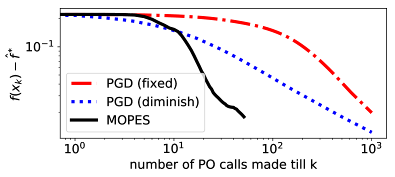
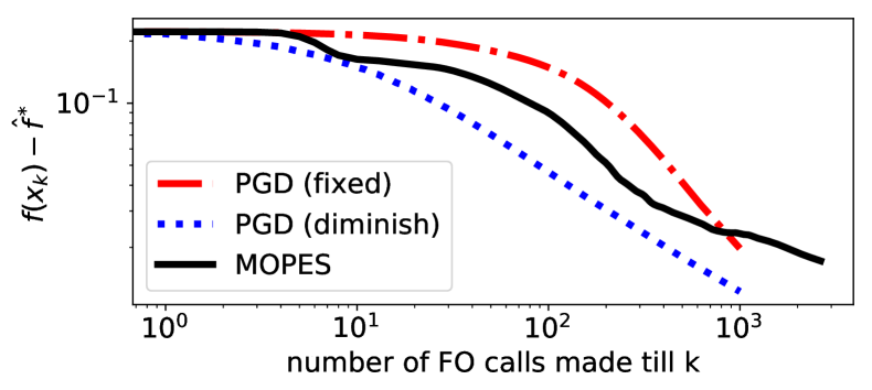
Figure 1: MOPES uses significantly fewer PO calls and comparable number of FO calls than PGD

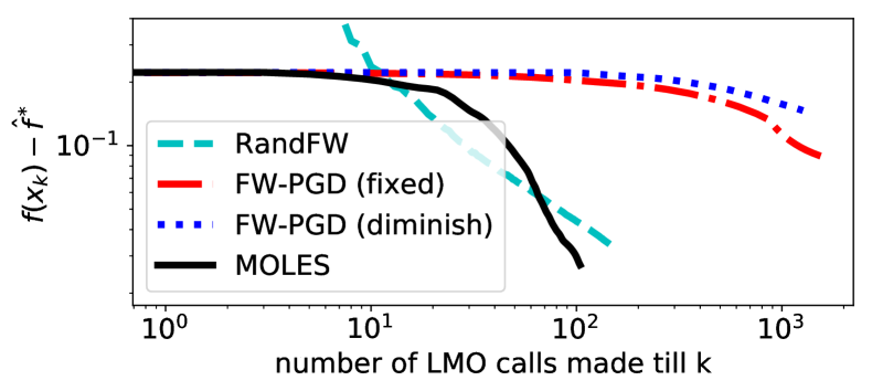
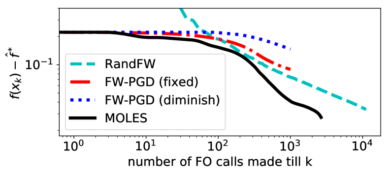
Figure 2: MOLES uses fewer LMO calls and similar number of FO calls than FW-PGD and RandFW

We experimentally evaluate MOPES (Algorithm 1) and MOLES (Algorithm 2) methods on a low rank SVM problem [85] of the form (11) on a subset of the Imagewoof 2.0 dataset [43]. The training data contains $n=400$ samples $\{(A_{i},y_{i})\}_{i=1}^{n}$ where $A_{i}$ is a $224\times 224$ grayscale image labeled using $y_{i}\in\{0,1\}$. Note that the effective dimension is $d=50176$. We use $r=0.1$ as nuclear norm ball radius of $\mathcal{X}$. First, we compare the PO and FO efficiencies of MOPES with those of PGD with a fixed and PGD with a diminishing stepsize. In Figure 2 we plot the mean (over 10 runs) sub-optimality gap: $f(x_{k})-\hat{f}^{*}$, of the iterates against the number of PO (top) and FO (bottom) calls, respectively, used to obtain that iterate. Next, we compare the LMO and FO efficiencies of MOLES with those of FW-PGD (see Algorithm 3 in Appendix B.2) and Randomized Frank-Wolfe (RandFW) [54, Theorem 5] methods with a fixed and diminishing stepsizes. In Figure 2 we plot the mean (over 10 runs) sub-optimality gap: $f(x_{k})-\hat{f}^{*}$, of the iterates against the number of LMO (top) and FO (bottom) calls, respectively, used to obtain that iterate. In both these plots, while MOPES/MOLES and baselines have comparable FO-CC, MOPES/MOLES is significantly more efficient in the number of PO/LMO calls, matching our Theorems 1 and 2. As the nuclear norm ball has a non-trivial projection/LMO, PO-CC/LMO-CC will dominate the total run-time as $m$ becomes larger for $X\in{\mathbb{R}}^{m\times m}$. Note that matrix mirror descent [47] would also require $O(\varepsilon^{-2})$ SVD based proximal operations. We provide additional experimental details in Appendix D.

6 Conclusion

We study a canonical problem in optimization: minimizing a nonsmooth Lipschitz continuous convex function over a convex constraint set. We assume that the function is accessed with a first-order oracle (FO) and the set is accessed with either a projection oracle (PO) or a linear minimization oracle (LMO). In this general setting, we address the fundamental question of reducing the number of accesses to the function and the set. When using projections, we introduce MOPES, and show that it finds an $\varepsilon$-suboptimal solution with ${\mathcal{O}}(\varepsilon^{-2})$ FO calls and ${\mathcal{O}}(\varepsilon^{-1})$ PO calls. This is optimal in the number of FO calls and significantly improves over competing methods in the number of PO calls (see Table 1). When using linear minimizations, we introduce MOLES, and show that it finds an $\varepsilon$-suboptimal solution with ${\mathcal{O}}(\varepsilon^{-2})$ FO and LMO calls. This is optimal in both the number of PO and the number of LMO calls. This resolves a question left open since [84] on designing the optimal Frank-Wolfe type algorithm for nonsmooth functions.

The two properties we need of the superset $\mathcal{X}^{\prime}\supseteq\mathcal{X}$ are that (a) it is easy to project onto $\mathcal{X}^{\prime}$ and (b) $f$ is $G$-Lipschitz on $\mathcal{X}^{\prime}$. In our paper, we choose $\mathcal{X}^{\prime}$ to be a Euclidean ball (which is easy to project to) but any other choice of $\mathcal{X}^{\prime}$ which satisfies the above properties works just as well. For example, if $f$ is Lipschitz everywhere, we can set $\mathcal{X}^{\prime}={\mathbb{R}^{d}}$ and ignore the explicit projection to $\mathcal{X}^{\prime}$ in algorithm 1 of Algorithm 1. However, even if $f$ is $G$-Lipschitz inside the constraint $\mathcal{X}$, $f$ could (i) have unbounded Lipschitz constant, or (ii) be undefined just outside of $\mathcal{X}$. Thus an $\mathcal{X}^{\prime}$ satisfying our requirements may not exist. In our experiments, we do not explicitly project onto $\mathcal{X}^{\prime}$ (algorithm 1) but still observed that $\|x_{k}-x_{k}^{\prime}\|={\mathcal{O}}(G\lambda)={\mathcal{O}}(\varepsilon)$ and small, which implies that the iterates $x_{k}^{\prime}$ are close to $\mathcal{X}$. This hints that we may only need Lipschitzness over a much smaller set, say $\mathcal{X}+B(0,{\mathcal{O}}(G\lambda))$, but we do not have a proof for this conjecture. Theoretically, we can work around the issue (ii) above by minimizing the convex extension $f_{\mathcal{X}}:\mathbb{R}^{d}\rightarrow\mathbb{R}$ of the function $f$ from the set $\mathcal{X}$, defined as $f_{\mathcal{X}}(x^{\prime})\mathrel{\mathop{:}}=\max_{x\in\mathcal{X}}\max_{g\in\partial f(x)}f(x)+\left\langle g,x^{\prime}-x\right\rangle$. The extension $f_{\mathcal{X}}$ has the same value as $f$ inside $\mathcal{X}$ and is $G$-Lipschitz everywhere. Therefore the minimization problems $\min_{x\in\mathcal{X}}f(x)$ and $\min_{x\in\mathcal{X}}f_{\mathcal{X}}(x^{\prime})$ are equivalent. However, it is not clear if we can estimate/approximate the gradients of $f_{\mathcal{X}}$ efficiently. We did not find any relevant prior work and leave this question for future work.

Another possible direction of future work is developing $\varepsilon$-horizon oblivious algorithms, where we need not fix $K$ and $\varepsilon$ a priori. In our experiments, we observed that varying $\lambda$ according to $\lambda_{k}=O(\frac{D_{\mathcal{X}}}{Gk})$ and $\beta_{k}=\frac{4}{\lambda_{k}k}$ works just as well as fixing it. However, obtaining any guarantee for this scheme seems challenging and again seems to require the bound $\|x_{k}-x_{k}^{\prime}\|={\mathcal{O}}(G\lambda_{k})$.

Broader Impact

As this is foundational research that is theoretical in nature, it is hard to predict any foreseeable societal consequence.

Appendix

Appendix A Supplementary results

A.1 Intuition behind the design of MOPES and a failed attempt

In this section we study the main ideas behind the design of MOPES method through a failed attempt. Only for the section, for simplicity, we assume that $\mathcal{X}^{\prime}$ is the whole vector space, and $f$ is $G$ Lipschitz in $\mathcal{X}^{\prime}$. Recall that we want to solve the problem (5),

$$\min_{x\in\mathcal{X},x^{\prime}\in\mathcal{X}^{\prime}}[\Psi_{\lambda}(x,x^{\prime})=\psi_{\lambda}(x,x^{\prime})+f(x^{\prime})]\,.$$ (12)

Notice that this is a composite objective which is a sum of a $2/\lambda$-smooth function $\psi_{\lambda}$ and a nonsmooth function $f$. This implies that, if we have access to the proximal operator (recall Definition 3) for $f$

$${\rm prox}_{f/t}(z)\mathrel{\mathop{:}}=\arg\min_{x\in\mathcal{X}^{\prime}}f(x)+\frac{t}{2}\|x-z\|^{2}\,,$$ (13)

then theoretically we can solve this problem using accelerated proximal gradient algorithm (APGD) [8, 67, 81], which has the following update rule

$$\begin{aligned} \beta_{k}&\leftarrow{4}/{\lambda k}\;,\;\gamma_{k}\leftarrow{2}/{(k+1)}\\ ({y}_{k},{y}_{k}^{\prime})&\leftarrow\left(1-\gamma_{k}\right)({x}_{k-1},{x}_{k-1}^{\prime})+\gamma_{k}({z}_{k-1},{z}_{k-1}^{\prime})\\ {z}_{k}&\leftarrow\mathcal{P}_{\mathcal{X}}\left({z}_{k-1}-\nabla_{x}\psi_{\lambda}({{y}_{k}},{y}_{k}^{\prime})/\beta_{k}\right)\\ {z}_{k}^{\prime}&\leftarrow{\rm prox}_{f/\beta_{k}}\left({z}_{k-1}^{\prime}-\nabla_{x^{\prime}}\psi_{\lambda}({{y}_{k}},{y}_{k}^{\prime})/\beta_{k}\right)\\ ({x}_{k},{x}_{k}^{\prime})&\leftarrow\left(1-\gamma_{k}\right)({x}_{k-1},{x}_{k-1}^{\prime})+\gamma_{k}({z}_{k},{z}_{k}^{\prime})\end{aligned}\,,$$ (APGD)

for some stepsize $1/\beta_{k}$ and iterate weight $\gamma_{k}$.

Notice that this update rule is different from the standard accelerated schemes, because the latter either first update the primal variables $(x,x^{\prime})$ and then extrapolate the dual variables $(z,z^{\prime})$ [65] or simultaneously update them both [69, 57], whereas (APGD), which is fashioned along the lines of [81], first updates $(z,z^{\prime})$ using proximal step and then extrapolates these to update $(x,x^{\prime})$. Advantage of [81] over the standard rule are three fold; former only needs one proximal step per variable (as opposed to two in [69, 57]) per iteration (which makes it practically faster), or keeps the dual and middle iterates $z_{k}$, $y_{k}$ feasible (as opposed to [65, (2.2.17)]), and can easily handle stochastic FO and constraints [53]. Another reason for the choice, which will be evident later on, is that, our update rule can simultaneously provide the optimal complexity for the smooth $\psi_{\lambda}$ and nonsmooth $f$ parts of the composite function, $\Psi_{\lambda}$ (5) [55].

With the right choice of $\beta_{k}$, $\gamma_{k}$, (APGD) can find an $\varepsilon$-approximate solution to the problem (5), $({x}_{K},{x}_{K}^{\prime})$, in ${\cal O}({\sqrt{2/\lambda\varepsilon}})$ steps. Now if we choose $\lambda={\cal O}({\varepsilon})$, we can show that ${x}_{K}$ is also an ${\cal O}({\varepsilon})$ solution of our original nonsmooth constrained problem (1). This is formalized in the Lemma 2. Thus applying (APGD) on (5) with $\lambda=\varepsilon/G^{2}$ gives us an $\varepsilon$ solution to the original problem (1) using only $K={\cal O}({G/\varepsilon})$ projections, which is a significant improvement over the ${\cal O}({G^{2}/\varepsilon^{2}})$ PO calls used by the standard subgradient method.

For a general $G$-Lipschitz convex function $f$, we cannot solve ${\rm prox}_{f/\beta_{k}}$ exactly, and hence we resort to some approximate solution. We emphasize here that it is not immediately evident that we can implement an inexact ${\rm prox}$ operator, and still maintain that the total number of FO calls used by this inexact APGD method match the optimal lowerbound ${\cal O}({G^{2}/\varepsilon^{2}})$ [64, 65]. Perhaps surprisingly, this is achieved using the Gradient Sliding method [55], which proposes a specific form of an inexact APGD. Note that the constrained variable $x\in\mathcal{X}$ is not an input to the nonsmooth part $f$ of $\Psi_{\lambda}$, which means that approximately resolving the ${\rm prox}$ operator ${\rm prox}_{f/t}$ does not require any projection.

As an intermediate algorithm we first present (IAPGD), which is derived from (APGD) but replaces the proximal update of ${z}_{k}^{\prime}$ with an inexact resolution for prox operator ${\rm prox}_{f/\beta_{k}}$ up to an approximation error of $\delta$. Notice that $\delta=0$, implies that $z_{k}$ is an exact resolution of the operation ${\rm prox}_{f/\beta_{k}}(\hat{z}_{k}^{\prime})$. The specific choice of the approximation error is important, as other notions of approximation error of the proximal operator in the context of APGD (such as those in [77]) do not explicitly control the distance $\|x^{\prime}-{z}_{k}^{\prime}\|^{2}$ which is crucial for our guarantee. Although with $\delta=\varepsilon$, (IAPGD) would require ${\mathcal{O}}(1/\varepsilon^{3})$ FO calls, we provide the details of its analysis, in the next theorem, as it showcases some of the ideas behind the design of our our main algorithm (Algorithm 4).

$$\begin{aligned} &\text{Use the update rule of \eqref{eq:apgd_update}, but replace ${\rm prox}$ step by the following:}\\ &\text{find ${z}_{k}^{\prime}$ satisfying the following for all $x^{\prime}\in\mathcal{X}^{\prime}$}\\ &\frac{\beta_{k}}{2}\|x^{\prime}-{z}_{k}^{\prime}\|^{2}+f({z}_{k}^{\prime})+\frac{\beta_{k}}{2}\|{z}_{k}^{\prime}-\hat{z}_{k}^{\prime}\|^{2}\;\leq\;f({x}^{\prime})+\frac{\beta_{k}}{2}\|{x}^{\prime}-\hat{z}_{k}^{\prime}\|^{2}+\delta\;,\\ &\text{ where }\hat{z}_{k}^{\prime}=({z}_{k-1}^{\prime}-\nabla_{x^{\prime}}\psi_{\lambda}({{y}_{k}},{y}_{k}^{\prime})/\beta_{k})\end{aligned}$$ (IAPGD)

Theorem 3.

Let $f:\mathcal{X}^{\prime}\to\mathbb{R}$ be a $G$-Lipschitz continuous convex function and $\mathcal{X}\subseteq\mathcal{X}^{\prime}$ be any convex set with a diameter $D_{\mathcal{X}}$ and projection oracle $\mathcal{P}_{\mathcal{X}}$. If we choose $\lambda=\varepsilon/G^{2}$ and $\delta=\varepsilon$, then after $K={\mathcal{O}}({GD_{\mathcal{X}}/\varepsilon})$ iterations of the IAPGD update rule, initialized with $y_{0}^{\prime}=y_{0}=x_{0}^{\prime}=x_{0}$, finds ${x}_{K}\in\mathcal{X}$ satisfying $f({x}_{K})-\min_{x\in\mathcal{X}}f(x)\leq{\varepsilon}$. Further, ${\mathcal{O}}({G^{2}D_{\mathcal{X}}^{2}/\varepsilon^{2}})$ iterations of a standard subgradient method ensures the condition in (IAPGD). In total, this algorithm requires ${\mathcal{O}}({G^{3}D_{\mathcal{X}}^{3}/\varepsilon^{3}})$ FO calls and ${\mathcal{O}}(GD_{\mathcal{X}}/\varepsilon)$ PO calls.

Remarks: Even though IAPGD only achieves a FO-CC of ${\mathcal{O}}(1/\varepsilon^{3})$, the main take away from this result should be that with this right choice for approximate resolvent of the proxoperator ${\rm prox}_{f/\beta_{k}}$ (IAPGD), we can achieve ${\mathcal{O}}(1/\varepsilon)$ PO-CC. This is exploited by our MOPES method (Algorithm 1) which uses a more efficient Prox-Slide procedure [55] to approximately resolve the prox operator, so as to obtain a PO-CC of ${\mathcal{O}}(1/\varepsilon)$ while still maintaining the optimal FO-CC o ${\mathcal{O}}(1/\varepsilon^{2})$.

Proof of Theorem 3.

Now consider the following potential (Lyapunov) function from [6] for arbitrary $x\in\mathcal{X}$ and $x^{\prime}\in\mathcal{X}^{\prime}$:

$$\Phi_{k}\mathrel{\mathop{:}}=k(k+1)(\Psi_{\lambda}({x}_{k},{x}_{k}^{\prime})-\Psi_{\lambda}(x,x^{\prime}))+({4}/{\lambda})\|({z}_{k},{z}_{k}^{\prime})-(x,x^{\prime})\|^{2}$$ (14)

We will prove that this potential satisfy the following approximate descent condition $\Phi_{k}\leq\Phi_{k-1}+k\varepsilon$ as follows. Notice that by $2/\lambda$-smoothness and convexity of $\psi_{\lambda}$

$$\psi_{\lambda}({x}_{k},{x}_{k}^{\prime})\leq\; \psi_{\lambda}({y}_{k},{y}_{k}^{\prime})+\left\langle\nabla_{k},({x}_{k},{x}_{k}^{\prime})-({y}_{k},{y}_{k}^{\prime})\right\rangle+\frac{1}{\lambda}\|({x}_{k},{x}_{k}^{\prime})-({y}_{k},{y}_{k}^{\prime})\|^{2}$$

$$\leq\; (1-\gamma_{k})\psi_{\lambda}({x}_{k-1},{x}_{k-1}^{\prime})+$$

$$\gamma_{k}[\psi_{\lambda}({y}_{k},{y}_{k}^{\prime})+\left\langle\nabla_{k},({z}_{k},{z}_{k}^{\prime})-({y}_{k},{y}_{k}^{\prime})\right\rangle+\frac{\gamma_{k}}{\lambda}\|({z}_{k},{z}_{k}^{\prime})-({z}_{k-1},{z}_{k-1}^{\prime})\|^{2}]$$ (15)

where we use the shorthand $\nabla_{k}\mathrel{\mathop{:}}=[\nabla_{k,x}^{T}\nabla_{k,x^{\prime}}^{T}]^{T}\mathrel{\mathop{:}}=[\nabla_{x}\psi_{\lambda}({y}_{k},{y}_{k}^{\prime})^{T}\;\nabla_{x^{\prime}}\psi_{\lambda}({y}_{k},{y}_{k}^{\prime})^{T}]^{T}$. Now combining this with $f({x}_{k}^{\prime})\leq(1-\gamma_{k})f({x}_{k-1}^{\prime})+\gamma_{k}f({z}_{k}^{\prime})$ (convexity) and $\gamma_{k}/\lambda\leq\beta_{k}/2$ we get that

$$k(k+1)\Psi_{\lambda}({x}_{k},{x}_{k}^{\prime})$$

$$\leq\; k(k-1)\Psi_{\lambda}({x}_{k-1},{x}_{k-1}^{\prime})+2k\psi_{\lambda}({y}_{k},{y}_{k}^{\prime})+2k[\left\langle\nabla_{k,x},{z}_{k}-{y}_{k}\right\rangle+\frac{\beta_{k}}{2}\|{z}_{k}-{z}_{k-1}\|^{2}]$$

$$2k[f({z}_{k}^{\prime})+\left\langle\nabla_{k,x^{\prime}},{z}_{k}^{\prime}-{y}_{k}^{\prime}\right\rangle+\frac{\beta_{k}}{2}\|{z}_{k}^{\prime}-{z}_{k-1}^{\prime}\|^{2}]$$

$$\leq\; k(k-1)\Psi_{\lambda}({x}_{k-1},{x}_{k-1}^{\prime})+2k\psi_{\lambda}({y}_{k},{y}_{k}^{\prime})+$$

$$2k[\left\langle\nabla_{k,x},x-{y}_{k}\right\rangle+\frac{\beta_{k}}{2}(\|{z}_{k-1}-x\|^{2}-\|{z}_{k}-x\|^{2})]$$

$$2k[f(x^{\prime})+\left\langle\nabla_{k,x^{\prime}},x^{\prime}-{y}_{k}^{\prime}\right\rangle+\frac{\beta_{k}}{2}(\|{z}_{k-1}^{\prime}-x^{\prime}\|^{2}-\|{z}_{k}^{\prime}-x^{\prime}\|^{2})+\varepsilon]$$

$$\leq\; k(k-1)\Psi_{\lambda}({x}_{k-1},{x}_{k-1}^{\prime})+2k\Psi_{\lambda}(x,x^{\prime})+$$

$$(4/\lambda)(\|({z}_{k-1},{z}_{k-1}^{\prime})-(x,x^{\prime})\|^{2}-\|({z}_{k},{z}_{k}^{\prime})-(x,x^{\prime})\|^{2})+k\varepsilon\,,$$ (16)

where the second inequality uses the definition of projection and the $\varepsilon$-approximate resolution of the proximal operator (IAPGD), and the last inequality again uses convexity of $\psi_{\lambda}$. This proves that $\Phi_{k}\leq\Phi_{k-1}+k\varepsilon$, which directly implies that

$$\Psi_{\lambda}({x}_{K},{x}_{K}^{\prime})-\Psi_{\lambda}(x,x^{\prime})\leq\frac{4(\|x_{0}-x\|^{2}+\|x_{0}-x^{\prime}\|^{2})}{\lambda K(K+1)}+\frac{1}{K(K+1)}\sum_{k=1}^{K}k\varepsilon$$ (17)

Setting $x^{\prime}=x$, choosing $\lambda=\varepsilon/G^{2}$ and $K={\mathcal{O}}({GD_{\mathcal{X}}/\varepsilon})$ gives us $\Psi_{\lambda}({x}_{k},{x}_{k}^{\prime})-f(x)\leq\varepsilon/2$. Then by Lemma 2 we get that $f({x}_{k})-\min_{x\in\mathcal{X}}f(x)\leq\varepsilon$. For each inner problem the standard (unconstrained) proximal subgradient method applied on $\min_{x^{\prime}\in\mathcal{X}^{\prime}}f(x^{\prime})+(\beta_{k}/2)\|x^{\prime}-({z}_{k-1}^{\prime}-\nabla_{k,x^{\prime}}/\beta_{k})\|^{2}$, initialized with $x_{0}$ (for ease of argument), can achieve this error using ${\mathcal{O}}({G^{2}\|x_{0}-\widehat{x}_{\lambda}(x)\|^{2}/\varepsilon^{2}})={\mathcal{O}}({G^{2}D_{\mathcal{X}}^{2}/\varepsilon^{2}})$ FO calls (Lemma 3, in Appendix B.1). Thus the algorithm uses totally ${\mathcal{O}}({GD_{\mathcal{X}}/\varepsilon})$ projections and ${\mathcal{O}}({G^{3}D_{\mathcal{X}}^{3}/\varepsilon^{3}})$ subgradients. ∎

Appendix B Supporting results

B.1 Proximal Subgradient method

Lemma 3 (proximal subgradient descent).

Consider the regularized optimization problem

$$\min_{u}[f_{\beta,x}(u)\mathrel{\mathop{:}}=f(u)+(\beta/2)\|u-x\|^{2}]$$ (18)

and the proximal subgradient method’s update rule

$$u_{t+1} =\mathop{\mathrm{argmin}}_{u}[F_{t}(u)\mathrel{\mathop{:}}=\left\langle g_{t},u-x\right\rangle+(1/{2\eta})\|u-u_{t}\|^{2}+\beta/2\|u-x\|^{2}]$$

$$=u_{t}-(\eta/(1+\eta\beta))(g_{t}+\beta(u_{t}-x))$$ (19)

where $g_{t}\in\partial f(u_{t})$ and $\eta$ is the effective stepsize. Now, if $\eta=2\,G^{2}\|u_{0}-u\|/\sqrt{T}$ and $\widetilde{u}_{T}=\frac{1}{T}\sum_{t=0}^{T-1}u_{t+1}$, then for any $u$

$$\frac{\beta}{2}\|\widetilde{u}_{T}-u\|^{2}+f_{\beta,x}(\widetilde{u}_{T})-f_{\beta,x}(u) \leq\frac{2\,G\,\|u_{0}-u\|}{\sqrt{T}}$$ (20)

Proof.

Let $u$ be an arbitrary feasible point. By convexity and $G$-Lipschitzness of $f$,

$$f(u_{t+1})-f(u) =f(u_{t+1})-f(u_{t})+f(u_{t})-f(u)$$

$$\leq\left\langle g_{t+1},u_{t+1}-u_{t}\right\rangle+\left\langle g_{t},u_{t}-u\right\rangle$$

$$=\left\langle g_{t},u_{t+1}-u_{t}\right\rangle+\left\langle g_{t+1}-g_{t},u_{t+1}-u_{t}\right\rangle+\left\langle g_{t},u_{t}-u\right\rangle$$

$$\leq\left\langle g_{t},u_{t+1}-u\right\rangle+2G\,\|u_{t+1}-u_{t}\|\,,$$ (21)

As $u_{t+1}$ is the minimizer of a $(\beta+1/\eta)$-strong convexity update objective $F_{t}$ and since, we get that

$$\big{(}\frac{\beta}{2}+\frac{1}{2\eta}\big{)}\|u_{t+1}-u\|^{2}+F_{t}(u_{t+1}) \leq F_{t}(u)$$ (22)

Now summing up (21), sand (22) we get

$$\frac{\beta}{2}\|u_{t+1}-u\|^{2}+f_{\beta,x}(u_{t+1})-f_{\beta,x}(u) \leq\frac{1}{2\eta}(\|u_{t}-u\|^{2}-\|u_{t+1}-u\|^{2})+$$

$$\;\;\;2G\,\|u_{t+1}-u_{t}\|-\frac{1}{2\eta}\|u_{t+1}-u_{t}\|^{2}$$

$$\leq\frac{1}{2\eta}(\|u_{t}-u\|^{2}-\|u_{t+1}-u\|^{2})+{2\,G^{2}\eta}$$

$$\implies\frac{1}{T}\sum_{t=0}^{T-1}\frac{\beta}{2}\|u_{t+1}-u\|^{2}+f_{\beta,x}(u_{t+1})-f_{\beta,x}(u) \leq\frac{1}{2\eta T}(\|u_{0}-u\|^{2}-\|u_{T}-u\|^{2})+{2\,G^{2}\eta}$$

$$\frac{\beta}{2}\|\widetilde{u}_{T}-u\|^{2}+f_{\beta,x}(\widetilde{u}_{T})-f_{\beta,x}(u) \leq$$ (23)

where the second inequality follows from $ax-x^{2}/2b\leq a^{2}b/2$, the third inequality is obtained by summing over $t=0,\ldots,T-1$, and the third inequality uses Jensen’s inequality. Choosing $T=2\,G\,\|u_{0}-u\|/\sqrt{T}$, we get the desired result

$$\frac{\beta}{2}\|\widetilde{u}_{T}-u\|^{2}+f_{\beta,x}(\widetilde{u}_{T})-f_{\beta,x}(u) \leq\frac{2\,G\,\|u_{0}-u\|}{\sqrt{T}}$$ (24)

∎

B.2 Frank-Wolfe projected subgradient method FW-PGD (Algorithm 3)

Here we provide the details of the Frank-Wolfe based projected subgradient method (Algorithm 3) used in the experiments. The main idea is to use some competitive LMO based method to approximate the projection step in the standard projected subgradient method. The following theorem gives some guarantees for the output of the Algorithm 3.

Input: $f$, $\mathcal{X}$, $G$, $D_{\mathcal{X}}$, $x_{0}$, $K$,

0.1

0.2 for $k=0,\ldots,K-1$ do

0.3       Set $\widehat{g}_{k}=\text{SFO}\left(x_{k}\right)$

0.4       Using any competitive LMO based algorithm (e.g. Frank-Wolfe method [28] or ${\rm CndG}$ procedure [56, Algo. 1]), approximately solve the projection problem

$$x_{k+1}\approx\mathop{\mathrm{argmin}}_{x\in\mathcal{X}}\left\langle\widehat{g}_{k},x\right\rangle+\frac{1}{2\alpha_{k}}\|x-x_{k}\|^{2}=\mathop{\mathrm{argmin}}_{x\in\mathcal{X}}\frac{1}{2\alpha_{k}}\|x-(x_{k}-\alpha_{k}\cdot\widehat{g}_{k})\|^{2}\,,$$ (25)

ensuring that the Wolfe duality gap [45] of the above problem at $u_{\Pi}$ satisfies

$$x\max_{s\in\mathcal{X}}\left\langle\widehat{g}_{k}+1/\alpha_{k}\left(x_{k+1}-{x_{k}}\right),{x}_{k+1}-s\right\rangle\leq\eta_{k}\,$$ (26)

Output: $\bar{x}_{K}=\frac{\sum_{k=0}^{K-1}\alpha_{k}x_{k}}{\sum_{k=0}^{K-1}\alpha_{k}}$

Algorithm 3 Frank-Wolfe projected subgradient method using LMO

Theorem 4.

Let $f:\mathcal{X}^{\prime}\to\mathbb{R}$ be a $G$-Lipschitz continuous proper l.s.c. convex function, and $\mathcal{X}\subseteq\mathcal{X}^{\prime}$ be some closed convex subset of $\mathbb{R}^{d}$ with diameter $D_{\mathcal{X}}$. Then after $K$ iterations, the Algorithm 3 projection tolerance $\eta_{k}=(G^{2}+\sigma^{2})\alpha_{k}$, stepsize $\alpha_{k}=\frac{D_{\mathcal{X}}}{2\sqrt{G^{2}+\sigma^{2}}\sqrt{K}}$ and outputs $\bar{x}_{K}\in\mathcal{X}$ satisfying

$$\mathbb{E}[f\left(\bar{x}_{K}\right)]-f(x^{*})\leq \frac{2\sqrt{G^{2}+\sigma^{2}}D_{\mathcal{X}}}{\sqrt{K}}$$ (27)

Further, the algorithm uses $K$ SFO calls and $O(K^{2})$ LMO calls.

Proof.

Using the Wolfe duality gap guarantee we get that for any $x\in\mathcal{X}$

$$\left\langle\widehat{g}_{k}+\frac{1}{\alpha_{k}}\left(x_{k+1}-{x_{k}}\right),{x}_{k+1}-x\right\rangle\leq\eta_{k}\,.$$ (28)

By rearranging the terms above we get that

$$\left\langle\widehat{g}_{k},{x}_{k}-x\right\rangle \leq\frac{1}{2\alpha_{k}}(\|x_{k}-x\|^{2}-\|x_{k+1}-x\|^{2})-\frac{1}{2\alpha_{k}}\|x_{k+1}-x_{k}\|^{2}+\left\langle\widehat{g}_{k},{x}_{k}-x_{k+1}\right\rangle+\eta_{k}$$

$$\leq\frac{1}{2\alpha_{k}}(\|x_{k}-x\|^{2}-\|x_{k+1}-x\|^{2})-\frac{1}{2\alpha_{k}}\|x_{k+1}-x_{k}\|^{2}+\|\widehat{g}_{k}\|\|{x}_{k}-x_{k+1}\|+\eta_{k}$$

$$\leq\frac{1}{2\alpha_{k}}(\|x_{k}-x\|^{2}-\|x_{k+1}-x\|^{2})+\frac{\alpha_{k}}{2}\|\widehat{g}_{k}\|^{2}+\eta_{k}\,,$$ (29)

where the last inequality uses the fact that $-(a/2)z^{2}+bz\leq b^{2}/2a$ for all $a,b,z\in\mathbb{R}$. Next, multiplying by $\alpha_{k}$ and summing the above inequality over $k=0,\ldots,K-1$ and dividing by $\sum_{{k^{\prime}}=0}^{K-1}\alpha_{k^{\prime}}$ we get

$$\sum_{k=0}^{K-1}\alpha_{k}\left\langle\widehat{g}_{k},{x}_{k}-x\right\rangle \leq\frac{1}{2}(\|x_{0}-x\|^{2}-\|x_{K}-x\|^{2})+\sum_{k=0}^{K-1}{\alpha_{k}^{2}}(\frac{\|\widehat{g}_{k}\|^{2}}{2}+\frac{\eta_{k}}{\alpha_{k}})\,,$$ (30)

Now taking expectation w.r.t. all the stochasticity in $\{\widehat{g}_{k}\}_{k=0}^{K-1}$ on both sides and using, the towering conditional expectation property $\mathbb{E}[a]=\mathbb{E}[\mathbb{E}[a\,|\,x_{k}]]$, and $\mathbb{E}[\widehat{g}_{k}\,|\,x_{k}]=g_{k}\in\partial f(x_{k})$ and $\mathbb{E}[\|\widehat{g}_{k}\|^{2}\,|\,x_{k}]\leq 2(G^{2}+\sigma^{2})$ we get

$$\sum_{k=0}^{K-1}\alpha_{k}\mathbb{E}[\left\langle g_{k},{x}_{k}-x\right\rangle] \leq\frac{1}{2}\|x_{0}-x\|^{2}+\sum_{k=0}^{K-1}{\alpha_{k}^{2}}((G^{2}+\sigma^{2})+\frac{\eta_{k}}{\alpha_{k}})\,,$$ (31)

Next diving by $\sum_{{k^{\prime}}=0}^{K-1}\alpha_{k^{\prime}}$, using convex affine lower bound of $f$ at $x_{k}$ and Jensen’s inequality we get

$$\sum_{k=0}^{K-1}\frac{\alpha_{k}}{\sum_{k^{\prime}=0}^{K-1}\alpha_{k^{\prime}}}\mathbb{E}[f({x}_{k})-f(x)] \leq\frac{\frac{1}{2}\|x_{0}-x\|^{2}+\sum_{k=0}^{K-1}\alpha_{k}^{2}((G^{2}+\sigma^{2})+\frac{\eta_{k}}{\alpha_{k}})}{\sum_{{k^{\prime}}=0}^{K-1}\alpha_{k^{\prime}}}$$

$$\mathbb{E}\bigg{[}f\bigg{(}\sum_{k=0}^{K-1}\frac{\alpha_{k}\cdot{x}_{k}}{\sum_{{k^{\prime}}=0}^{K-1}\alpha_{k^{\prime}}}\bigg{)}\bigg{]}-f(x) \leq$$ (32)

Next if we choose $\eta_{k}=\alpha_{k}(G^{2}+\sigma^{2})$, and set $x=x^{*}\in\mathop{\mathrm{argmin}}_{x^{\prime}\in\mathcal{X}}f(x^{\prime})$ and $\alpha_{k}=\frac{D_{\mathcal{X}}}{2\sqrt{G^{2}+\sigma^{2}}\sqrt{K}}$ we get

$$\mathbb{E}\bigg{[}f\bigg{(}\sum_{k=0}^{K-1}\frac{\alpha_{k}\cdot{x}_{k}}{\sum_{{k^{\prime}}=0}^{K-1}\alpha_{k^{\prime}}}\bigg{)}\bigg{]}-f(x^{*}) \leq\frac{\frac{1}{2}D_{\mathcal{X}}^{2}+\sum_{k=0}^{K-1}\alpha_{k}^{2}\cdot 2(G^{2}+\sigma^{2})}{\sum_{{k^{\prime}}=0}^{K-1}\alpha_{k^{\prime}}}$$

$$=\frac{2\sqrt{G^{2}+\sigma^{2}}D_{\mathcal{X}}}{\sqrt{K}}$$ (33)

Clearly the algorithm uses $K$ SFO calls. At step $k$ when approximating the projection using an LMO based method, after using $\hat{T}_{k}=\lceil\frac{7D_{\mathcal{X}}^{2}}{\alpha_{k}^{2}(G^{2}+\sigma^{2})}\rceil$ LMO calls in the Approx-Proj procedure, the Wolfe duality gap (38) is at most $\lceil\frac{6(1/\alpha_{k})D_{\mathcal{X}}^{2}}{\hat{T}_{k}}\rceil\leq\alpha_{k}(G^{2}+\sigma^{2})$ if we use CndG procedure [56, Theorem 2.2(c)] or $\lceil\frac{7(1/\alpha_{k})D_{\mathcal{X}}^{2}}{\hat{T}_{k}}\rceil\leq\alpha_{k}(G^{2}+\sigma^{2})$ if we use the standard Frank-Wolfe algorithm [45, Theorem 2]. Therefore the total number of linear minimization oracle calls made by the algorithm is

$$\sum_{k=0}^{K-1}\hat{T}_{k}=\sum_{k=0}^{K-1}\frac{7D_{\mathcal{X}}^{2}}{\alpha_{k}^{2}(G^{2}+\sigma^{2})}+K=28K^{2}+K=O(K^{2})$$ (34)

where we use the given choice for $\alpha_{k}=\frac{D_{\mathcal{X}}}{2\sqrt{G^{2}+\sigma^{2}}\sqrt{K}}$. ∎

Appendix C Proofs of the main results

C.1 Proof of Lemma 2

Proof.

First we prove part $(i)$. By definitions of $\Psi_{\lambda}$ (5) and $f_{\lambda}$ (Definition 3), we have $\min_{x\in\mathcal{X}}\min_{x\in\mathcal{X}^{\prime}}\Psi_{\lambda}(x,x^{\prime})=\min_{x\in\mathcal{X}}f_{\lambda}(x)$. By Lemma 1(a), we also can show that $\min_{x\in\mathcal{X}}f_{\lambda}(x)\leq\min_{x\in\mathcal{X}}f(x)$.

For part $(ii)$, first we show the following.

$$\mathbb{E}f_{\lambda}(x_{\varepsilon})=\mathbb{E}\Psi_{\lambda}(x_{\varepsilon},\widehat{x}_{\lambda}(x_{\varepsilon}))=\mathbb{E}\min_{x^{\prime}(x_{\varepsilon})}\Psi_{\lambda}(x_{\varepsilon},x^{\prime}(x_{\varepsilon})) \leq\mathbb{E}_{\bar{x}_{K}}\Psi_{\lambda}(x_{\varepsilon},\mathbb{E}_{x_{\varepsilon}^{\prime}|x_{\varepsilon}}x_{\varepsilon}^{\prime})$$

$$\leq\mathbb{E}_{x_{\varepsilon}}\mathbb{E}_{x_{\varepsilon}^{\prime}|x_{\varepsilon}}\Psi_{\lambda}(x_{\varepsilon},x_{\varepsilon}^{\prime})$$

$$=\mathbb{E}\Psi_{\lambda}(x_{\varepsilon},x_{\varepsilon}^{\prime})$$ (35)

Finally, combining the above inequality with Lemma 1(c) we get the desired result

$$\mathbb{E}f(x_{\varepsilon}) \leq\mathbb{E}f_{\lambda}(x_{\varepsilon})+G^{2}\lambda/2\leq\mathbb{E}\Psi_{\lambda}(x_{\varepsilon},x_{\varepsilon}^{\prime})+G^{2}\lambda/2$$ (36)

∎

C.2 Analysis of MOPES (Algorithm 1) and MOLES (Algorithm 2) method

Instead of separately analyzing MOPES and MOLES, we first analyze a more general algorithm, Algorithm 4, which has the following guarantee.

Input: $f$, $\mathcal{X}$, $\mathcal{X}^{\prime}$, $G$, $D_{\mathcal{X}}$, $R$, $x_{0}$, $K$, $\tilde{D}$, $\lambda$, $\{\eta_{k}\in\mathbb{R}_{+}\}_{k\in[K]}$

0.1

0.2 Set ${x}_{0}^{\prime}={z}_{0}^{\prime}={x}_{0}={z}_{0}=x_{0}$

0.3 for $k=1,\ldots,K$ do

0.4       Set $\lambda_{k}=\lambda$, $\beta_{k}=\frac{4}{\lambda_{k}k}\;,\;\gamma_{k}=\frac{2}{k+1}\,,\text{ and }T_{k}=\Big{\lceil}{\frac{(4G^{2}+\sigma^{2})\lambda^{2}Kk^{2}}{2\tilde{D}}}\Big{\rceil}$

0.5      

0.6      Set $({y}_{k},{y}_{k}^{\prime})=\left(1-\gamma_{k}\right)\cdot({x}_{k-1},{x}_{k-1}^{\prime})+\gamma_{k}\cdot({z}_{k-1},{z}_{k-1}^{\prime})$

0.7      

      Set ${z}_{k}=\textnormal{{Approx-Proj}}\left(\nabla_{y_{k}}\Psi_{\lambda}(y_{k},y_{k}^{\prime}),{z}_{k-1},\beta_{k},\eta_{k}\right)$ // Note $\nabla_{y_{k}}\Psi_{\lambda}(y_{k},y_{k}^{\prime})=\frac{y_{k}-y_{k}^{\prime}}{\lambda}$

0.8      

      Set $\left({z}_{k}^{\prime},{\widetilde{z}}_{k}^{\prime}\right)=\text{{{Prox-Slide}}}\big{(}\nabla_{y_{k}^{\prime}}\psi_{\lambda}(y_{k},y_{k}^{\prime}),{z}_{k-1}^{\prime},\beta_{k},T_{k}\big{)}$

        // $\nabla_{y_{k}^{\prime}}\psi_{\lambda}(y_{k},y_{k}^{\prime})=\frac{{y}_{k}^{\prime}-{y}_{k}}{\lambda}$

0.9      

0.10      Set $({x}_{k},{x}_{k}^{\prime})=\left(1-\gamma_{k}\right)\cdot({x}_{k-1},{x}_{k-1}^{\prime})+\gamma_{k}\cdot({z}_{k},{\widetilde{z}}_{k}^{\prime})$

0.11      

Output: $({x}_{K},{x}^{\prime}_{K})$

0.12

0.13 Approx-Proj($g$, $u_{0}$, $\beta$, $\eta$) // Approx. resolve $\mathcal{P}_{\mathcal{X}}\big{(}u_{0}-g/\beta\big{)}$[56] :

0.14       Either using exact PO, $\mathcal{P}_{\mathcal{X}}$ (1) , or using any competitive LMO based algorithm (e.g. Frank-Wolfe method [28] or ${\rm CndG}$ procedure [56, Algo. 1]), approximately solve the projection problem

$$u_{\Pi}\approx\mathop{\mathrm{argmin}}_{u\in\mathcal{X}}\left\langle g,u\right\rangle+\frac{\beta}{2}\|u-u_{0}\|^{2}=\mathop{\mathrm{argmin}}_{u\in\mathcal{X}}\frac{\beta}{2}\|u-(u_{0}-g/\beta)\|^{2}\,,$$ (37)

ensuring that the Wolfe duality gap [45] of the above problem at $u_{\Pi}$ satisfies

$$\max_{s\in\mathcal{X}}\left\langle g+\beta\left(u_{\Pi}-{u_{0}}\right),{u}_{\Pi}-s\right\rangle\leq\eta_{k}\,$$ (38)

return $u_{\Pi}$

0.15

0.16 Prox-Slide($g$, $u_{0}$, $\beta$, $T$) // Approx. resolve ${{\rm prox}}_{f/\beta}\big{(}u_{0}-g/\beta\big{)}$[55] :

0.17       Set $\widetilde{u}_{0}=u_{0}$

0.18       for $t=1,\ldots,{T}$ do

0.19             Set $\theta_{t}=\frac{2(t+1)}{t(t+3)}$, $\ \ \widehat{g}_{t-1}=\text{SFO}\left(u_{t-1}\right)$ (3)

             Set $\widehat{u}_{t}=u_{t-1}-\frac{1}{(1+t/2)\beta}\cdot(\widehat{g}_{t-1}+\beta(u_{t-1}-(u_{0}-g/\beta)))$

              // subgradient method step for $\phi(u)\mathrel{\mathop{:}}=f(u)+\frac{\beta}{2}\|u-\big{(}u_{0}-\frac{g}{\beta}\big{)}\|^{2}$

             Set $u_{t}=\widehat{u}_{t}\cdot\min\left(1,R/\|{u_{t}}\|\right)$

              // projection of $\widehat{u}_{t}$ onto $\mathcal{X}^{\prime}$: $\mathcal{P}_{\mathcal{X}}^{\prime}(\mathbf{u}_{t})$

0.20             Set $\widetilde{u}_{t}=\big{(}1-\theta_{t}\big{)}\cdot\widetilde{u}_{t-1}+\theta_{t}\cdot u_{t}$

0.21            

0.22      return $(u_{T},\widetilde{u}_{T})$

0.23      

Algorithm 4 Moreau subgradient method for nonsmooth convex optimization using PO or LMO

Theorem 5.

Let $f:\mathcal{X}^{\prime}\to\mathbb{R}$ be a $G$-Lipschitz continuous proper l.s.c. convex function, and $\mathcal{X}\subseteq\mathcal{X}^{\prime}=B(0,R)$ be some convex subset contained inside the Euclidean ball of radius $R$ around origin. Then after $K$ iterations, the Algorithm 4 outputs ${x}_{K}\in\mathcal{X}$ satisfying

$$\mathbb{E}[f\left({x}_{K}\right)]-f(x^{*})\leq \frac{10\|x_{0}-x^{*}\|^{2}+8\tilde{D}}{\lambda K(K+1)}+\frac{\sum_{k=1}^{K}2k\,\eta_{k}}{K(K+1)}+G^{2}\frac{\lambda}{2}$$ (39)

for any choice of $\lambda>0$, $\tilde{D}>0$, and tolerance $\{\eta_{k}\}_{k\in[K]}$ (38).

Remarks: Before providing a proof for the above result we discuss some its implications. MOPES makes $K$ PO calls, one per outer step, and $\sum_{k=1}^{K}T_{k}={\mathcal{O}}(\lambda^{2}K^{4})$ SFO calls, one per inner step. The above analysis shows that we need to choose $\lambda=\varepsilon/G^{2}$, which is expected from Lemma 1. Since PO returns exact projections, the second term is zero with $\eta_{k}=0$. The target accuracy of $\varepsilon$ is achieved by tuning the first term, where we need to choose $K=\Theta(1/\sqrt{\lambda\varepsilon})$. Put together, this gives the desired ${\mathcal{O}}(\varepsilon^{-1})$ PO-CC and ${\mathcal{O}}(\varepsilon^{-2})$ SFO-CC for MOPES. A complete proof is provided in Section C.2.1.

When we have inexact projections in MOLES, we need $\eta_{k}=\Theta(1/k)$ to ensure that the second term is ${\mathcal{O}}(\varepsilon)$. At (outer) iteration $k$, this uses $\hat{T}=\Omega(K)$ iterations of Frank-Wolfe algorithm in FW-Based-Projection of Algorithm 2. MOLES makes $\sum_{k=1}^{K}{\mathcal{O}}(K)={\mathcal{O}}(K^{2})$ LMO calls, resulting in ${\mathcal{O}}(\varepsilon^{-2})$ LMO-CC as $K={\mathcal{O}}(1/\sqrt{\lambda\varepsilon})={\mathcal{O}}(1/\varepsilon)$. A complete proof is in Section C.2.2.

Proof of Theorem 5.

Now consider the following potential (Lyapunov) function:

$$\Phi_{k}\mathrel{\mathop{:}}=k(k+1)(\Psi_{\lambda}({x}_{k},{x}_{k}^{\prime})-\Psi_{\lambda}(x,x^{\prime}))+\frac{4}{\lambda}(\|{z}_{k}-x\|^{2}+\frac{(T_{k+1}+1)(T_{k+1}+2)}{T_{k+1}(T_{k+1}+3)}\|{z}_{k}^{\prime}-x^{\prime}\|^{2})$$ (40)

This is a slightly modified version of the following potential function for the standard AGD setting with a $2/\lambda$-smooth function $\Psi_{\lambda}$ [6]: $k(k+1)(\Psi_{\lambda}({x}_{k},{x}_{k}^{\prime})-\Psi_{\lambda}(x,x^{\prime}))+\frac{4}{\lambda}(\|{z}_{k}-x\|^{2}+\|{z}_{k}^{\prime}-x^{\prime}\|^{2})$. Notice that the modification factor

$$\frac{(T_{k+1}+1)(T_{k+1}+2)}{T_{k+1}(T_{k+1}+3)}\leq\frac{3}{2}={\mathcal{O}}(1)$$ (41)

is upper-bounded by a constant when $1\leq T_{k}$. Below we prove that this potential satisfies the approximate descent guarantee: $\Phi_{k}\leq\Phi_{k-1}+k\eta_{k}+k\eta_{k}^{\prime}$, for some error $\eta_{k}^{\prime}$. First, notice that by $2/\lambda$-smoothness and convexity of $\psi_{\lambda}$

$$\psi_{\lambda}({x}_{k},{x}_{k}^{\prime})\leq\; \psi_{\lambda}({y}_{k},{y}_{k}^{\prime})+\left\langle\nabla_{k},({x}_{k},{x}_{k}^{\prime})-({y}_{k},{y}_{k}^{\prime})\right\rangle+\frac{1}{\lambda}\|({x}_{k},{x}_{k}^{\prime})-({y}_{k},{y}_{k}^{\prime})\|^{2}$$

$$\overset{}{=}\; (1-\gamma_{k})[\psi_{\lambda}({y}_{k},{y}_{k}^{\prime})+\left\langle\nabla_{k},({x}_{k-1},{x}_{k-1}^{\prime})-({y}_{k},{y}_{k}^{\prime})\right\rangle]$$

$$\gamma_{k}[\psi_{\lambda}({y}_{k},{y}_{k}^{\prime})+\left\langle\nabla_{k},({z}_{k},{\widetilde{z}}_{k}^{\prime})-({y}_{k},{y}_{k}^{\prime})\right\rangle+\frac{\gamma_{k}}{\lambda}\|({z}_{k},{\widetilde{z}}_{k}^{\prime})-({z}_{k-1},{z}_{k-1}^{\prime})\|^{2}]$$

$$\leq\; (1-\gamma_{k})\psi_{\lambda}({x}_{k-1},{x}_{k-1}^{\prime})+$$

$$\gamma_{k}[\psi_{\lambda}({y}_{k},{y}_{k}^{\prime})+\left\langle\nabla_{k},({z}_{k},{\widetilde{z}}_{k}^{\prime})-({y}_{k},{y}_{k}^{\prime})\right\rangle+\frac{\gamma_{k}}{\lambda}\|({z}_{k},{\widetilde{z}}_{k}^{\prime})-({z}_{k-1},{z}_{k-1}^{\prime})\|^{2}]$$ (42)

where we use the shorthand $\nabla_{k}\mathrel{\mathop{:}}=[\nabla_{k,x}^{T}\nabla_{k,x^{\prime}}^{T}]^{T}\mathrel{\mathop{:}}=[\nabla_{x}\psi_{\lambda}({y}_{k},{y}_{k}^{\prime})^{T}\;\nabla_{x^{\prime}}\psi_{\lambda}({y}_{k},{y}_{k}^{\prime})^{T}]^{T}$, and second inequality used Algorithms 4 and 4. Now combining this with $f({x}_{k}^{\prime})\leq(1-\gamma_{k})f({x}_{k-1}^{\prime})+\gamma_{k}f({\widetilde{z}}_{k}^{\prime})$ (using convexity of $f$ and Algorithm 4) and $\gamma_{k}/\lambda=2/(\lambda(k+1))\leq{2}/{(\lambda\,k)}=\beta_{k}/2$ (using Algorithm 4), and multiplying it with $k(k+1)$ we get that

$$k(k+1)\Psi_{\lambda}({x}_{k},{x}_{k}^{\prime})$$

$$\leq\; k(k-1)\Psi_{\lambda}({x}_{k-1},{x}_{k-1}^{\prime})+2k\psi_{\lambda}({y}_{k},{y}_{k}^{\prime})+2k[\left\langle\nabla_{k,x},{z}_{k}-{y}_{k}\right\rangle+\frac{\beta_{k}}{2}\|{z}_{k}-{z}_{k-1}\|^{2}]$$

$$2k[f({\widetilde{z}}_{k}^{\prime})+\left\langle\nabla_{k,x^{\prime}},{\widetilde{z}}_{k}^{\prime}-{y}_{k}^{\prime}\right\rangle+\frac{\beta_{k}}{2}\|{\widetilde{z}}_{k}^{\prime}-{z}_{k-1}^{\prime}\|^{2}]$$

$$=\; k(k-1)\Psi_{\lambda}({x}_{k-1},{x}_{k-1}^{\prime})+2k\psi_{\lambda}({y}_{k},{y}_{k}^{\prime})+2k[\left\langle\nabla_{k,x},{z}_{k}-{y}_{k}\right\rangle+\frac{\beta_{k}}{2}\|{z}_{k}-{z}_{k-1}\|^{2}]$$

$$2k[\phi_{k}({\widetilde{z}}_{k}^{\prime})-\phi_{k}(x^{\prime})+\frac{\beta_{k}}{2}\|x^{\prime}-{z}_{k-1}^{\prime}\|^{2}+f(x^{\prime})+\left\langle\nabla_{k,x^{\prime}},x^{\prime}-{y}_{k}^{\prime}\right\rangle]$$ (43)

where for brevity we use the notation

$$\phi_{k}(x^{\prime})\mathrel{\mathop{:}}=f\left(x^{\prime}\right)+\left\langle\nabla_{k,x^{\prime}},x^{\prime}\right\rangle+\frac{\beta_{k}}{2}\left\|x^{\prime}-{z}_{k-1}^{\prime}\right\|^{2}\,.$$ (44)

Now using the approximate optimality of ${z}_{k}$ through the bound on the Wolfe dual gap (38) we get,

$$\frac{\beta_{k}}{2}\left\|{z}_{k}-{z}_{k-1}\right\|^{2} =\frac{\beta_{k}}{2}\left\|{z}_{k-1}-{x}\right\|^{2}+\beta_{k}\left\langle{z}_{k}-{z}_{k-1},{z}_{k}-x\right\rangle-\frac{\beta_{k}}{2}\left\|{z}_{k}-{x}\right\|^{2}$$

$$\leq\frac{\beta_{k}}{2}\left\|{z}_{k-1}-{x}\right\|^{2}+\left\langle\nabla_{k,x},x-{z}_{k}\right\rangle+\eta_{k}-\frac{\beta_{k}}{2}\left\|{z}_{k}-{x}\right\|^{2}\,.$$ (45)

When ${z}_{k}$ is the exact projection (as in Algorithm 1) then the above inequality is satisfied with above $\eta_{k}=0$. Otherwise, with the LMO oracle we will later set $\eta_{k}={\mathcal{O}}(\varepsilon)$. Next we state the following lemma which provides a guarantee for the Prox-Slide procedure [55]. Here for rigorousness, we denote the iterates of the Prox-Slide procedure (Algorithm 4) called at the outer step $k$, with $\{u_{k,t}\}_{t}$. Similarly at the outer step $k$, we denote the stochastic subgradients used by the Prox-Slide procedure and the corresponding subgradient with $\{\widehat{g}_{k,t}\}_{t}$ and $\{g_{k,t}\}_{t}$, i.e. $g_{k,t}\mathrel{\mathop{:}}=\mathbb{E}[\widehat{g}_{k,t}|u_{k,t}]\in\partial f(u_{k,t})$ for all $k$ and $t$. A proof for this lemma is provided in Section C.2.3.

Proposition 2 ([55, Similar to Proposition 1]).

Let $\phi_{k}$ (44) be the minimization objective solved by Prox-Slide procedure at step $k$ of Algorithm 4. Then $({z}_{k}^{\prime},{\widetilde{z}}_{k}^{\prime})$ obtained after $T_{k}$ iterations of the procedure satisfy the following for any $x^{\prime}\in\mathcal{X}^{\prime}$,

$$\phi_{k}({\widetilde{z}}_{k}^{\prime})-\phi_{k}(x^{\prime}) \leq\frac{2}{T_{k}(T_{k}+3)}\frac{\beta_{k}}{2}\|{z}_{k-1}^{\prime}-x^{\prime}\|^{2}-\frac{(T_{k}+1)(T_{k}+2)}{T_{k}(T_{k}+3)}\frac{\beta_{k}}{2}\|{z}_{k}^{\prime}-x^{\prime}\|^{2}+$$

$$\;\;\;\;\;\frac{4\,\sum_{t=0}^{T_{k}-1}(2G+\|\delta_{k,t}\|)^{2}}{\beta_{k}T_{k}(T_{k}+3)}+\sum_{t=0}^{T_{k}-1}\frac{2(t+2)}{T_{k}(T_{k}+3)}\left\langle\delta_{k,t},x^{\prime}-u_{k,t}\right\rangle$$ (46)

where $\delta_{k,t}\mathrel{\mathop{:}}=\widehat{g}_{k,t}-g_{k,t}$ and $u_{k,t}$ are private inner variable of the Prox-Slide procedure.

Aside: Note that Prox-Slide procedure essentially applies $T_{k}$ steps of the proximal standard subgradient method to the $\phi_{k}$ (44), which is a composite function of a $G$-Lipschitz function $f$ and prox-friendly $\beta_{k}$-strongly convex quadratic. Finally the procedure outputs the average of its iterate ${\widetilde{z}}_{k}^{\prime}$ and its last iterate ${z}_{k}^{\prime}$. In the end we will set $T_{k}=\Theta(1/\varepsilon)$ and $K=\Theta(1/\varepsilon)$ so that total number of subgradients used by the algorithm be $\sum_{k=1}^{K}T_{k}={\mathcal{O}}(1/\varepsilon^{2})$.

Now substituting (45) and Proposition 2 into (43) we get

$$k(k+1)\Psi_{\lambda}({x}_{k},{x}_{k}^{\prime})\leq\; k(k-1)\Psi_{\lambda}({x}_{k-1},{x}_{k-1}^{\prime})+2k\psi_{\lambda}({y}_{k},{y}_{k}^{\prime})+$$

$$2k[\left\langle\nabla_{k,x},x-{y}_{k}\right\rangle+\frac{\beta_{k}}{2}(\|{z}_{k-1}-x\|^{2}-\|{z}_{k}-x\|^{2})+\eta_{k}]$$

$$2k[f(x^{\prime})+\left\langle\nabla_{k,x^{\prime}},x^{\prime}-{y}_{k}^{\prime}\right\rangle]+$$

$$2k[\frac{(T_{k}+1)(T_{k}+2)}{T_{k}(T_{k}+3)}\frac{\beta_{k}}{2}\|{z}_{k-1}^{\prime}-x^{\prime}\|^{2}-\frac{(T_{k}+1)(T_{k}+2)}{T_{k}(T_{k}+3)}\frac{\beta_{k}}{2}\|{z}_{k}^{\prime}-u\|^{2}+\eta_{k}^{\prime}]$$

$$\leq\; k(k-1)\Psi_{\lambda}({x}_{k-1},{x}_{k-1}^{\prime})+2k\Psi_{\lambda}(x,x^{\prime})+2k(\eta_{k}+\eta_{k}^{\prime})$$

$$\frac{4}{\lambda}(\|{z}_{k-1}-x\|^{2}-\|{z}_{k}-x\|^{2})$$

$$\frac{4}{\lambda}(\frac{(T_{k}+1)(T_{k}+2)}{T_{k}(T_{k}+3)}\|{z}_{k-1}^{\prime}-x^{\prime}\|^{2}-\frac{(T_{k+1}+1)(T_{k+1}+2)}{T_{k+1}(T_{k+1}+3)}\|{z}_{k}^{\prime}-x^{\prime}\|^{2})\,,$$ (47)

where we use the shorthand

$$\eta_{k}^{\prime}\mathrel{\mathop{:}}=\frac{4\,\sum_{t=0}^{T_{k}-1}(2G+\|\delta_{k,t}\|)^{2}}{\beta_{k}T_{k}(T_{k}+3)}+\sum_{t=0}^{T_{k}-1}\frac{2(t+2)}{T_{k}(T_{k}+3)}\left\langle\delta_{k,t},x^{\prime}-u_{k,t}\right\rangle\,,$$ (48)

and the last inequality uses convexity of $\psi_{\lambda}$ and $\Psi_{\lambda}=f+\psi_{\lambda}$, definition of $\beta_{k}$ (Algorithm 4), and the fact that

$$T_{k}\leq T_{k+1}\quad\text{(\lx@cref{creftypecap~refnum}{algo_line:envelope-subgrad-param-set})}\quad\text{, and }\quad\frac{(T_{k+1}+1)(T_{k+1}+2)}{T_{k+1}(T_{k+1}+3)}\leq\frac{(T_{k}+1)(T_{k}+2)}{T_{k}(T_{k}+3)}$$ (49)

This proves the approximate descent guarantee: $\Phi_{k}\leq\Phi_{k-1}+k(\eta_{k}+\eta_{k}^{\prime})$, which along with the facts: $1\leq T_{1}$ and ${z}_{0}={z}_{0}^{\prime}=x_{0}$ gives

$$\Psi_{\lambda}({x}_{K},{x}_{K}^{\prime})-\Psi_{\lambda}(x,x^{\prime})\leq \frac{4(\|x_{0}-x\|^{2}+(3/2)\|x_{0}-x^{\prime}\|^{2})}{\lambda K(K+1)}+\frac{\sum_{k=1}^{K}2k(\eta_{k}+\eta_{k}^{\prime})}{K(K+1)}$$ (50)

Now we take expectation, with respect to randomness in all the stochastic subgradients $((\widehat{g}_{k,i})_{i=1}^{T_{k}})_{k=1}^{K}$ used in the algorithm, on both sides of (50). Then the expectation of the error from the Prox-Slide procedure can be bounded as follows

$$\sum_{k=1}^{K}2k\mathbb{E}[\eta_{k}^{\prime}] =\sum_{k=1}^{K}2k\mathbb{E}[\frac{4\,\sum_{t=0}^{T_{k}-1}(2G+\|\delta_{k,t}\|)^{2}}{\beta_{k}T_{k}(T_{k}+3)}+\sum_{t=0}^{T_{k}-1}\frac{2(t+2)}{T_{k}(T_{k}+3)}\left\langle\delta_{k,t},u-u_{t}\right\rangle]$$

$$\leq\sum_{k=1}^{K}2k\frac{8\,(4G^{2}+\sigma^{2})}{(\frac{4}{\lambda k})(\frac{(4G^{2}+\sigma^{2})\lambda^{2}Kk^{2}}{2\tilde{D}})}+0$$

$$=\frac{8\tilde{D}}{\lambda}$$ (51)

where we use (48), linearity of expectation, $(a+b)^{2}\leq 2(a^{2}+b^{2})$, variance of stochastic gradient $\mathbb{E}[\|\delta_{k,t}\|^{2}|u_{k,t}]=\mathbb{E}[\|\widehat{g}_{k,t}-g_{k,t}\|^{2}|u_{k,t}]\leq\sigma^{2}$ (3), the value of $T_{k}$ from Algorithm 4, and the fact that expectation of the second term becomes zero, since $\mathbb{E}[\widehat{g}_{k,i-1}\,|\,u_{k,i-1}]=g_{k,i-1}$, which in turn implies

$$\mathbb{E}[\left\langle\delta_{k,t},x^{\prime}-u_{k,t}\right\rangle] =\mathbb{E}\big{[}\,\mathbb{E}[\left\langle\widehat{g}_{k,t}-g_{k,t},x^{\prime}-u_{k,t}\right\rangle\,|\,u_{k,t}]\,\big{]}s=\mathbb{E}[\left\langle 0,x^{\prime}-u_{k,i-1}\right\rangle]=0\;.$$ (52)

Aside: Note that, in the final guarantee, when we set $\lambda=\varepsilon/G^{2}$ and $K={\mathcal{O}}(1/\varepsilon)$, we are setting $T_{k}=\Theta(\varepsilon\,k^{2})={\mathcal{O}}(1/\varepsilon)$ and $1/\beta_{k}=\Theta(1/\varepsilon\,k)={\mathcal{O}}(1)$, so that the error from the Prox-Slide procedure is small enough. For example, at $k=K$, $\mathbb{E}[\eta_{K}]={\mathcal{O}}((G^{2}+\sigma^{2})/\beta_{K}T_{K})={\mathcal{O}}(\varepsilon)$.

Now taking expectation on both sides of (50) and using linearity of expectation and (51) we get that

$$\mathbb{E}[\Psi_{\lambda}\left({x}_{K},{x}_{K}^{\prime}\right)]-\Psi_{\lambda}(x,x^{\prime})\leq \frac{4(\|x_{0}-x\|^{2}+(3/2)\|x_{0}-x^{\prime}\|^{2}+2\tilde{D})}{\lambda K(K+1)}+\frac{\sum_{k=1}^{K}2k\,\eta_{k}}{K(K+1)}$$ (53)

Next setting $x^{\prime}=x=x^{*}\in\mathcal{X}\subseteq\mathcal{X}^{\prime}$ and using Lemma 2 and (5) we get that

$$\mathbb{E}[f\left({x}_{K}\right)]-f(x^{*})\leq\frac{10\|x_{0}-x^{*}\|^{2}+8\tilde{D}}{\lambda K(K+1)}+\frac{\sum_{k=1}^{K}2k\,\eta_{k}}{K(K+1)}+G^{2}\frac{\lambda}{2}$$ (54)

Aside: Note that, in the final guarantee, when we set $\lambda=\varepsilon/G^{2}$, the third term, which is the error from the Moreau smoothing becomes $\varepsilon/2$. Additionally, when $K={\mathcal{O}}(1/\varepsilon)$, first term above is ${\mathcal{O}}(\varepsilon)$. Further, when we set $T_{k}=\Theta(\varepsilon\,k^{2})={\mathcal{O}}(1/\varepsilon)$, we get $1/\beta_{k}={\mathcal{O}}(1/\varepsilon\,k)$ and $\mathbb{E}[\eta_{k}]={\mathcal{O}}(1/k)$ so that the second term is also ${\mathcal{O}}(\varepsilon)$. ∎

Next using the above result we derive the guarantees for MOPES (Algorithm 1) and MOLES (Algorithm 2) as corollaries of Theorem 5.

C.2.1 Proof of Theorem 1

Proof.

Notice that exact projection on Algorithm 1 of Algorithm 1 is equivalent to choosing $\eta_{k}=0$ in Algorithm 4. Then setting, $\eta_{k}=0$, and $\lambda=\varepsilon/G^{2}$ in Theorem 5 we get

$$\mathbb{E}[f\left({x}_{K}\right)]-f(x^{*})\leq\frac{G^{2}(10\|x_{0}-x^{*}\|^{2}+8\tilde{D})}{\varepsilon K(K+1)}+0+\frac{\varepsilon}{2}$$ (55)

Now, by using the given choices: $\tilde{D}=c\|x_{0}-x^{*}\|^{2}$ and $K=\lceil\frac{2\sqrt{10+8c}\,G\|x_{0}-x^{*}\|}{\varepsilon}\rceil$, we get

$$\mathbb{E}[f\left({x}_{K}\right)]-f(x^{*}) \leq\varepsilon$$ (56)

Then the number of PO calls made by the algorithm is $K={\mathcal{O}}({\frac{G\|x_{0}-x^{*}\|}{\varepsilon}})$ and the total number of SFO calls made subgradients made is

$$\sum_{k=1}^{K}T_{k}\leq\sum_{k=1}^{K}\left(\frac{(4G^{2}+\sigma^{2})\lambda^{2}Kk^{2}}{2\tilde{D}}+1\right) =\frac{(4G^{2}+\sigma^{2})\varepsilon^{2}K^{2}(K+1)(2K+1)}{12cG^{4}\|x_{0}-x^{*}_{\lambda}\|^{2}}+K$$

$$={\mathcal{O}}\left(\frac{(G^{2}+\sigma^{2})\|x_{0}-x^{*}\|^{2}}{\varepsilon^{2}}\right)\,,$$ (57)

where we used Algorithm 1 and the given choices for $\lambda$, $K$, and $\tilde{D}$. ∎

C.2.2 Proof of Theorem 2

Proof.

Notice that at step $k$ of Algorithm 2 choosing $\hat{T}=\lceil\frac{7KD_{\mathcal{X}}^{2}}{c^{\prime}\tilde{D}}\rceil={\mathcal{O}}(\frac{1}{\varepsilon})$ is equivalent to choosing $\eta_{k}=\frac{4c^{\prime}\tilde{D}}{\lambda Kk}$ in Algorithm 4 (see below). Therefore by setting, $\eta_{k}=\frac{4c^{\prime}\tilde{D}}{\lambda Kk}={\mathcal{O}}(\frac{1}{k})$, and $\lambda=\varepsilon/G^{2}$ in Theorem 5 we get

$$\mathbb{E}[f\left({x}_{K}\right)]-f(x^{*})\leq \frac{G^{2}(10\|x_{0}-x^{*}\|^{2}+8\tilde{D}+8c^{\prime}\tilde{D})}{\varepsilon K(K+1)}+\frac{\varepsilon}{2}$$ (58)

Now, by using the given choices: $\tilde{D}=c\|x_{0}-x^{*}\|^{2}$ and $K=\lceil\frac{2\sqrt{10+8c(1+c^{\prime})}G\|x_{0}-x^{*}\|}{\varepsilon}\rceil$, in the (58) we get

$$\mathbb{E}[f\left({x}_{K}\right)]-f(x^{*}) \leq\varepsilon$$ (59)

Then using the similar arguments as in proof of Theorem 2, we can show that $K={\mathcal{O}}({\frac{G\|x_{0}-x^{*}\|}{\varepsilon}})$ and the total number of SFO calls made is $\sum_{k=1}^{K}T_{k}={\mathcal{O}}({\frac{(G^{2}+\sigma^{2})\|x_{0}-x^{*}\|^{2}}{\varepsilon^{2}}})$.

Finally we calculate the total number of LMO calls made. At outer step $k$ of Algorithm 2, after using $\hat{T}=\lceil\frac{7KD_{\mathcal{X}}^{2}}{c^{\prime}\tilde{D}}\rceil$ LMO calls in the Approx-Proj procedure, the Wolfe duality gap (38) is at most $\lceil\frac{6\beta_{k}D_{\mathcal{X}}^{2}}{\hat{T}}\rceil\leq\frac{4c^{\prime}\tilde{D}}{\lambda Kk}=\eta_{k}$ if we use CndG procedure [56, Theorem 2.2(c)] or $\lceil\frac{7\beta_{k}D_{\mathcal{X}}^{2}}{\hat{T}}\rceil\leq\frac{4c^{\prime}\tilde{D}}{\lambda Kk}=\eta_{k}$ if we use the standard Frank-Wolfe algorithm [45, Theorem 2]. Therefore the total number of linear minimization oracle calls made by the algorithm is

$$K\hat{T}=\frac{7K^{2}D_{\mathcal{X}}^{2}}{cc^{\prime}\|x_{0}-x^{*}\|^{2}}+K={\mathcal{O}}\Big{(}\frac{G^{2}D_{\mathcal{X}}^{2}}{\varepsilon^{2}}\Big{)}\,,$$ (60)

where we used Algorithm 1 and the given choices for $K$ and $\tilde{D}$. ∎

C.2.3 Proof of Proposition 2: Analysis of Prox-Slide (Algorithm 4) procedure

Proof.

We analyze the Prox-Slide procedure for a fixed $k$, therefore we drop $k$ from $\phi_{k}$, $u_{k,t}$, $\widehat{g}_{k,t}$, and $\delta_{k,t}$, which are denoted here with $\phi$, $u_{t}$, $\widehat{g}_{t}$, and $\delta_{t}$. Prox-Slide has the following update steps.

$$\theta_{t} =\frac{2(t+1)}{t(t+3)}\,,\;\;\widehat{g}_{t-1}=\text{SFO}\left(u_{t-1}\right)$$ (61)

$$\widehat{u}_{t} =u_{t-1}-\frac{1}{(1+t/2)\beta}\cdot(\widehat{g}_{t-1}+\beta(u_{t-1}-(u^{\prime}-g/\beta)))$$ (62)

$$u_{t} =\widehat{u}_{t}\cdot\min(1,2R/\|\widehat{u}_{t}\|)$$ (63)

$$\widetilde{u}_{t} =\left(1-\theta_{t}\right)\widetilde{u}_{t-1}+\theta_{t}u_{t}$$ (64)

By convexity and $G$-Lipschitzness of $f$ in $\mathcal{X}^{\prime}$, for any $u\in\mathcal{X}^{\prime}$, we get

$$f(u_{t+1})-f(u) =f(u_{t+1})-f(u_{t})+f(u_{t})-f(u)$$

$$\leq\left\langle g_{t+1},u_{t+1}-u_{t}\right\rangle+\left\langle g_{t},u_{t}-u\right\rangle$$

$$=\left\langle\widehat{g}_{t},u_{t+1}-u_{t}\right\rangle+\left\langle g_{t+1}-g_{t}-\delta_{t},u_{t+1}-u_{t}\right\rangle+\left\langle\widehat{g}_{t},u_{t}-u\right\rangle-\left\langle\delta_{t},u_{t}-u\right\rangle$$

$$\leq\left\langle\widehat{g}_{t},u_{t+1}-u\right\rangle+(2G+\|\delta_{t}\|)\,\|u_{t+1}-u_{t}\|+\left\langle\delta_{t},u-u_{t}\right\rangle\,,$$ (65)

where we used the fact that $\delta_{t}=\widehat{g}_{t}-g_{t}$. Notice that $u_{t}=\widehat{u}_{t}\cdot\min(1,2R/\|\widehat{u}_{t}\|)$ is the projection of $\widehat{u}_{t}$ onto $\mathcal{X}^{\prime}=B(0,2R)$. Therefore, using Algorithm 4, we can re-write Prox-Slide update as

$$u_{t+1} =\mathop{\mathrm{argmin}}_{u\in\mathcal{X}^{\prime}}\frac{(t+3)\beta}{4}\;\|u-\widehat{u_{t}}\|^{2}$$

$$=\mathop{\mathrm{argmin}}_{u\in\mathcal{X}^{\prime}}\frac{(t+3)\beta}{4}\;\Big{\|}u-\Big{(}u_{t-1}-\frac{1}{(1+((t+1)/2)\beta}\cdot(\widehat{g}_{t-1}+\beta(u_{t-1}-(u_{0}-g/\beta)))\Big{)}\Big{\|}^{2}$$

$$=\mathop{\mathrm{argmin}}_{u\in\mathcal{X}^{\prime}}\Big{[}F_{t}(u)\mathrel{\mathop{:}}=\left\langle g,u\right\rangle+\left\langle\widehat{g}_{t},u\right\rangle+\frac{(t+1)\beta}{4}\|u-u_{t}\|^{2}+\frac{\beta}{2}\|u-u_{0}\|^{2}\Big{]}$$ (66)

By $\beta(t+3)/2$-strong convexity of the quadratic update objective $F_{t}(u)$ and the optimality of $u_{t+1}\in\mathop{\mathrm{argmin}}_{u\in\mathcal{X}^{\prime}}F_{t}(u)$, we get that for any $u\in\mathcal{X}^{\prime}$

$$\frac{\beta(t+3)}{4}\|u_{t+1}-u\|^{2}+F_{t}(u_{t+1}) \leq F_{t}(u)$$ (67)

We want to provide a lower bound on $\phi(u)$ 44 which is defined as follows, when using the private notation of the Prox-Slide procedure by setting $u=x^{\prime}$, $u^{\prime}=z_{k-1}$, $g=\nabla_{k,x^{\prime}}$, $\beta=\beta_{k}$.

$$\phi(u)\mathrel{\mathop{:}}=f\left(u\right)+\left\langle g,u\right\rangle+\frac{\beta}{2}\left\|u-u_{0}\right\|^{2}\,.$$ (68)

Now adding together (65) and (67) and using the definitions of $F_{t}$ and $\phi$ we get

$$\phi(u_{t+1})-\phi(u) \leq\frac{\beta}{2}(\frac{t+1}{2}\|u_{t}-u\|^{2}-\frac{t+3}{2}\|u_{t+1}-u\|^{2})+$$

$$\;\;\;\;\;(2G+\|\delta_{t}\|)\,\|u_{t+1}-u_{t}\|-\frac{\beta\,(t+1)}{4}\|u_{t+1}-u_{t}\|^{2}+\left\langle\delta_{t},u-u_{t}\right\rangle$$

$$\leq\frac{\beta}{2}(\frac{t+1}{2}\|u_{t}-u\|^{2}-\frac{t+3}{2}\|u_{t+1}-u\|^{2})+\frac{(2G+\|\delta_{t}\|)^{2}}{\beta\,(t+1)}+\left\langle\delta_{t},u-u_{t}\right\rangle$$ (69)

where the second inequality follows from $ax-bx^{2}/2\leq a^{2}/2b$. Now multiplying the above inequality is by $2(t+2)/T(T+3)$ and then summing over $t=\{0,\ldots,T-1\}$, we get

$$\sum_{t=0}^{T-1}\frac{2(t+2)}{T(T+3)}(\phi(u_{t+1})-\phi(u)) \leq\frac{\beta}{2}\frac{2}{T(T+3)}(\|u_{0}-u\|^{2}-\frac{(T+1)(T+2)}{2}\|u_{T}-u\|^{2})+$$

$$\;\;\;\;\;\frac{2}{T(T+3)}\frac{2\,\sum_{t=0}^{T-1}(2G+\|\delta_{t}\|)^{2}}{\beta}+\sum_{t=0}^{T-1}\frac{2(t+2)}{T(T+3)}\left\langle\delta_{t},u-u_{t}\right\rangle$$

$$\phi(\widetilde{u}_{T})-\phi(u) \leq$$ (70)

where the last inequality uses Jensen’s inequality and $\widetilde{u}_{T}=\sum_{t=1}^{T}\frac{2(t+1)}{T(T+3)}u_{t}$, last of which follows from Algorithms 4 and 4 as follows

$$\widetilde{u}_{T} =(1-\theta_{T})\widetilde{u}_{T-1}+\theta_{T}u_{T}$$

$$=\frac{(T-1)(T+2)}{T(T+3)}((1-\theta_{T-1})\widetilde{u}_{T-2}+\theta_{T-1}u_{T-1})+\frac{2(T+1)}{T(T+3)}u_{T}$$

$$=\frac{(T-2)(T+1)}{T(T+3)}\widetilde{u}_{T-2}+\frac{2(T)}{T(T+3)}u_{T-1}+\frac{2(T+1)}{T(T+3)}u_{T}$$

$$\;\;\vdots$$

$$=\sum_{t=1}^{T}\frac{2(t+1)}{T(T+3)}u_{t}$$ (71)

Finally we get the desired result by setting $\phi=\phi_{k}$, $\beta=\beta_{k}$, $T=T_{k}$, $u_{0}={\widetilde{z}}_{k-1}^{\prime}$, $u=x^{\prime}$, $u_{t}=u_{k,t}$, $\widetilde{u}_{T}={\widetilde{z}}_{k}^{\prime}$, and ${u}_{T}={z}_{k}$ we get the desired inequality

$$\phi_{k}({\widetilde{z}}_{k}^{\prime})-\phi_{k}(x^{\prime}) \leq\frac{2}{T_{k}(T_{k}+3)}\frac{\beta_{k}}{2}\|{z}_{k-1}^{\prime}-x^{\prime}\|^{2}-\frac{(T_{k}+1)(T_{k}+2)}{T_{k}(T_{k}+3)}\frac{\beta_{k}}{2}\|{z}_{k}^{\prime}-x^{\prime}\|^{2}+$$

$$\;\;\;\;\;\frac{4\,\sum_{t=0}^{T_{k}-1}(2G+\|\delta_{k,t}\|)^{2}}{\beta_{k}T_{k}(T_{k}+3)}+\sum_{t=0}^{T_{k}-1}\frac{2(t+2)}{T_{k}(T_{k}+3)}\left\langle\delta_{k,t},x^{\prime}-u_{k,t}\right\rangle$$ (72)

∎

C.3 Proof of Lemma 1

We re-write $f_{\lambda}(x)$ as minimum value of a $\frac{1}{\lambda}$-strong convex function $\phi_{\lambda,x}$ as follows

$$f_{\lambda}(x)=\min_{x^{\prime}\in\mathcal{X}^{\prime}}\bigg{[}\phi_{\lambda,x}(x^{\prime})\mathrel{\mathop{:}}=f(x^{\prime})+\frac{1}{2\lambda}\|x-x^{\prime}\|^{2}\bigg{]}\,.$$ (73)

Note that $\phi_{\lambda,x}(\cdot)$ is a $(1/\lambda)$-strongly convex function as $f$ is convex and $(1/\lambda)\|\cdot-x\|^{2}$ is strongly convex, and $f_{\lambda}(x)=\min_{x^{\prime}\in\mathcal{X}^{\prime}}\phi_{\lambda,x}(x^{\prime})$.
(a) The existence and uniqueness of $\hat{x}_{\lambda}(x)\in\mathcal{X}^{\prime}$ follows from the strong convexity of $\phi_{\lambda,x}(\cdot)$ and the fact that $f$ is a proper convex function. Then $f(\hat{x}_{\lambda}(x))\leq\phi_{\lambda,x}(\hat{x}_{\lambda}(x))=\min_{x^{\prime}\in\mathcal{X}^{\prime}}\phi_{\lambda,x}(x^{\prime})=f_{\lambda}(x)\leq\phi_{\lambda,x}(x)=f(x)$.
(b) Let $g_{x}\mathrel{\mathop{:}}={(x-\hat{x}_{\lambda}(x))}/\lambda$ for any $x\in{\mathbb{R}^{d}}$. By $(1/\lambda)$-strong convexity of $\phi_{\lambda,x}(x^{\prime})$ and $\hat{x}_{\lambda}(x)=\mathop{\mathrm{argmin}}_{x^{\prime}\in\mathcal{X}^{\prime}}\phi_{\lambda,x}(x^{\prime})$, we have, for any $x^{\prime}\in\mathcal{X}^{\prime}$, that

$$\phi_{\lambda,x}(x^{\prime}) \geq\phi_{\lambda,x}(\hat{x}_{\lambda}(x))+\|{x^{\prime}-\hat{x}_{\lambda}(x)}\|^{2}/2\lambda$$

$$\iff f(x^{\prime})+\|{x^{\prime}-x}\|^{2}/2\lambda \geq f(\hat{x}_{\lambda}(x))+\|{x^{\prime}-\hat{x}_{\lambda}(x)}\|^{2}/2\lambda+\|{x^{\prime}-\hat{x}_{\lambda}(x)}\|^{2}/2\lambda$$

$$\iff f(x^{\prime}) \geq f(\hat{x}_{\lambda}(x))+\left\langle g_{x},x^{\prime}-\hat{x}_{\lambda}(x)\right\rangle$$ (74)

Using this, for any $x,y\in\mathbb{R}^{d}$ we get

$$f_{\lambda}(y)-f_{\lambda}(x) =f(\hat{x}_{\lambda}(y))-f(\hat{x}_{\lambda}(x))+(\|\hat{x}_{\lambda}(y)-y\|^{2}-\|\hat{x}_{\lambda}(x)-x\|^{2})/{2\lambda}$$

$$\geq\left\langle g_{x},\hat{x}_{\lambda}(y)-\hat{x}_{\lambda}(x)\right\rangle+{\lambda/2}(\|g_{y}\|^{2}-\|g_{x}\|^{2})=\left\langle g_{x},y-x\right\rangle+\lambda/2\|g_{x}-g_{y}\|^{2}$$ (75)

By instantiating the above for $y\leftarrow x$, $x\leftarrow y$, we also get $f_{\lambda}(y)-f_{\lambda}(x)\leq\left\langle g_{y},y-x\right\rangle-\lambda/2\|g_{x}-g_{y}\|^{2}$. Combining these two inequalities

$$0\leq\lambda/2\|g_{y}-g_{x}\|^{2}\leq f_{\lambda}(y)-f_{\lambda}(x)-\left\langle g_{x},y-x\right\rangle \leq-\lambda/2\|g_{y}-g_{x}\|^{2}+\left\langle g_{y}-g_{x},y-x\right\rangle$$

$$\leq-\lambda/2\|g_{y}-g_{x}\|^{2}+\|g_{y}-g_{x}\|\|y-x\|$$

$$\leq\|y-x\|^{2}/2\lambda$$ (76)

This implies that $\lim_{y\to x}(f_{\lambda}(y)-f_{\lambda}(x)-\left\langle g_{x},y-x\right\rangle)/\|y-x\|=0$. Thus $f_{\lambda}$ is Frechet differentiable with gradient $\nabla f_{\lambda}(x)=g_{x}=(x-\hat{x}_{\lambda}(x))/\lambda$. The above inequality also implies $f_{\lambda}$ is convex and $1/\lambda$-smooth.
(c) Let $x\in\mathcal{X}^{\prime}$. Using $1/\lambda$-strong convexity of $\phi_{\lambda,x}$ and $\hat{x}_{\lambda}(x)\in\mathop{\mathrm{argmin}}_{x^{\prime}\in\mathcal{X}^{\prime}}\phi_{\lambda,x}(x^{\prime})$, and $G$-Lipschitzness of $f$ in $\mathcal{X}^{\prime}$, we get

$$\|x-\hat{x}_{\lambda}(x)\|^{2}/2\lambda\leq\phi_{\lambda,x}(x)-\phi_{\lambda,x}(\hat{x}_{\lambda}(x)) =f(x)-f_{\lambda}(x)$$

$$=f(x)-f(\hat{x}_{\lambda}(x))-\|x-\hat{x}_{\lambda}(x)\|^{2}/2\lambda$$

$$\leq G\|\hat{x}_{\lambda}(x)-x\|-\|x-\hat{x}_{\lambda}(x)\|^{2}/2\lambda\leq G^{2}\lambda/2\;.\qed$$

Appendix D Additional details for the experiments in Section 5

For all the experiments we randomly and uniformly sample a point $x_{0}$ from the surface of the nuclear norm ball of radius $r$. For all the figures where we plot the estimated sub-optimality gap: $f(x_{k})-\hat{f}^{*}$, where $\hat{f}^{*}$ is the estimated minimum function value calculated by running the PGD method for a large number of iterations. We plot the mean (standard error is negligible) of the sub-optimality gap over 10 runs using 10 different initial points $x_{0}$’s (same 10 initial points for all algorithms).

For experiments in Figures 2 and 2, we use a subset of the Imagewoof 2.0 dataset [43], which in itself is a subset of the Imagenet dataset [24]. The training data, contains $n=400$ samples $\{(A_{i},y_{i})\}_{i=1}^{n}$ where $A_{i}$ is a $224\times 224$ grayscale image of one of the two types of dogs (classes n$02087394$ and n$02115641$ in Imagenet dataset) labeled using $y_{i}\in\{0,1\}$. Note that the effective dimension is $d=224\times 224=50176$). These grayscale images are generated from the raw $8$-bit RGB Imagewoof images using the Pillow python image-processing library [21], by $(i)$ resizing to $256\times 256$ pixels: resize(256,256), $(ii)$ cropping to the central $224\times 224$ pixels: crop(16,16,240,240), $(iii)$ converting to the grayscale: convert(mode=‘L’), and $(iv)$ normalizing by $255.0$ so that the pixel values lie in range $[0,1]$. For incorporating bias scalar into the SVM model we also zero-pad the training images with an additional column and row of zeros to the right and the bottom of the image array $A_{i}$. We use $r=0.1$ as nuclear norm ball radius of $\mathcal{X}$, thus $D_{\mathcal{X}}=0.2$. We have access to a deterministic FO.

In Figure 2, we use a Lipschitz constant of $G=50$. For MOPES we set $c=40$ and $\varepsilon=5.0$, and for PGD we use two stepsize schemes: ($i$) fixed stepsize $D_{\mathcal{X}}/(G\sqrt{K})$ with $K=10^{3}$ and ($ii$) diminishing stepsize $D_{\mathcal{X}}/(G\sqrt{k})$ with $K=10^{3}$.

In Figure 2, we use a Lipschitz constant of $G=50$. For MOLES we set $c=40$, $c^{\prime}=1$ and $\varepsilon=5.0$. For FW-PGD we use two stepsize schemes: ($i$) fixed stepsize $D_{\mathcal{X}}/(G\sqrt{K})$ with $K=10^{3}$ and ($ii$) diminishing stepsize $D_{\mathcal{X}}/(G\sqrt{k})$ with $K=10^{3}$. Both of these stepsize schemes use a projection tolerance of $\eta_{k}G^{2}/2$. For RandFW we use the standard parameter choices as given in [54, Theorem 5] with $K=150$.

In practice, in the deterministic setup with FO, at outer-step $k$, we can use the following criterion for stopping the Prox-Slide (Algorithm 1) procedure early at some $t\geq\widehat{T}_{k-1}$ (defined recursively below with $\widehat{T}_{0}=1$) and $t\leq T_{k}$. Let $\phi_{k}(x^{\prime})\mathrel{\mathop{:}}=f\left(x^{\prime}\right)+\left\langle\nabla_{k,x^{\prime}},x^{\prime}\right\rangle+\frac{\beta_{k}}{2}\left\|x^{\prime}-{z}_{k-1}^{\prime}\right\|^{2}$ and $\widetilde{g}_{t}\in\partial f(\widetilde{u}_{t})$. Now if

$$\max_{x^{\prime}\in\mathcal{X}}\; \left\langle\widetilde{g}_{t}+\nabla_{k,x^{\prime}},\widetilde{u}_{t}-x^{\prime}\right\rangle-\frac{(t+1)(t+2)}{t(t+3)}{\beta_{k}}\left\langle u_{t}-{z}_{k-1}^{\prime},x^{\prime}\right\rangle$$

$$\leq\frac{8\,(4G^{2}+\sigma^{2})}{\beta_{k}(T_{k}+3)}-\frac{\beta_{k}}{2}\|\widetilde{u}_{t}-{z}_{k-1}^{\prime}\|^{2}+\frac{(t+1)(t+2)}{t(t+3)}\frac{\beta_{k}}{2}(\|{z}_{k-1}^{\prime}\|^{2}-\|u_{t}\|^{2})$$ (77)

then we stop the procedure, set $\widehat{T}_{k}=t$ and return $(u_{t},\widetilde{u}_{t})$. This implies that for $({z}_{k}^{\prime},{\widetilde{z}}_{k}^{\prime})=(u_{t},\widetilde{u}_{t})$

$$\phi_{k}({\widetilde{u}}_{t})-\phi_{k}(x^{\prime}) \leq\frac{2}{\widehat{T}_{k}(\widehat{T}_{k}+3)}\frac{\beta_{k}}{2}\|{z}_{k-1}^{\prime}-x^{\prime}\|^{2}-\frac{(\widehat{T}_{k}+1)(\widehat{T}_{k}+2)}{\widehat{T}_{k}(\widehat{T}_{k}+3)}\frac{\beta_{k}}{2}\|u_{t}-x^{\prime}\|^{2}+$$

$$\;\;\;\;\;\frac{4\,\sum_{t=0}^{T_{k}-1}(2G)^{2}}{\beta_{k}T_{k}(T_{k}+3)}$$ (78)

for all $x^{\prime}\in\mathcal{X}$. Now the only change we need to make in the analysis of Theorem 5 is the change of the potential (40) to

$$\Phi_{k}\mathrel{\mathop{:}}=k(k+1)(\Psi_{\lambda}({x}_{k},{x}_{k}^{\prime})-\Psi_{\lambda}(x,x^{\prime}))+\frac{4}{\lambda}(\|{z}_{k}-x\|^{2}+\frac{(\widehat{T}_{k+1}+1)(\widehat{T}_{k+1}+2)}{\widehat{T}_{k+1}(\widehat{T}_{k+1}+3)}\|{z}_{k}^{\prime}-x^{\prime}\|^{2})$$ (79)

The LHS of (77) is an linear optimization problem whose solution can be easily found as

$$\text{LMO}\left(\widetilde{g}_{t}+\nabla_{k,x^{\prime}}+\frac{(t+1)(t+2)}{t(t+3)}{\beta_{k}}(u_{t}-{z}_{k-1}^{\prime})\right)$$

$$= \lim_{\alpha\to\infty}\text{PO}\left(-\alpha\bigg{(}\widetilde{g}_{t}+\nabla_{k,x^{\prime}}+\frac{(t+1)(t+2)}{t(t+3)}{\beta_{k}}(u_{t}-{z}_{k-1}^{\prime})\bigg{)}\right)\,.$$ (80)

We also use a slightly modified $T_{k}=\Big{\lceil}{\frac{2G^{2}\lambda^{2}Kk^{2}}{2\tilde{D}}}\Big{\rceil}$ for our experiments, since the deterministic FO we use, ensures this choice gets the same guarantees as given in our theorems. Also, in our implementation we do not explicitly project ${z}_{k}$ onto $\mathcal{X}^{\prime}$, as in practice this does not seem needed.

In practice, we can eliminate the need for selecting $\varepsilon$ of MOPES by employing $\varepsilon$-doubling trick with warm restarts, which can increase the worse-case iteration complexity by a factor of at most $2$ but oftentimes will accelerate the convergence [80, Algorithm 6].

Appendix E Additional details for applications

We refer to [73] for some more nonsmooth problems which can be solved using an LMO. In the following subsections, we compare the analytical complexities for solving some of the applications mentioned in Section 4, using different algorithms.

E.1 $\ell_{1}$ norm constrained SVM

For simplicity, we work with the vector version of the matrix problems and replace nuclear norm constraint with the $\ell_{1}$ norm constraint. The standard $\ell_{1}$ norm constrained soft-margin SVM can be formulated as the the following optimization problem:

$$\min_{x\in\mathbb{R}^{d}}f(x)=\frac{1}{n}\sum_{i=1}^{n}[f_{i}(x)=\max(0,1-\left\langle x,a_{i}\right\rangle)]$$

$$\text{subject to }\;\;\;\|x\|_{1}\leq\lambda$$ (81)

where $a_{i}\in\mathbb{R}^{d}$ captures the $d$-dimensional feature vector multiplied by a binary class value in $\{-1,1\}$ and $\mathcal{X}=\{x\,|\,\|x\|_{1}\leq 1\}$ is the constraint set. We do not include any explicit bias term above, because it can always be incorporated into the model by augmenting $a_{i}$ with a constant dimension. We assume that $n$ is large and therefore we only have access to minibatched stochastic subgradients obtained through minibatching $d$ ($b={{o}}(n)$) uniformly sampled (with replacement) training samples. We assume that $f$ is $G_{p}$-Lipschitz continuous and the variance of any stochastic subgradient is upperbounded by $\sigma_{p}^{2}$, both calculated in $\ell_{p}$ norm $\|\cdot\|_{p}$, for $p=1,2$. We define $q\mathrel{\mathop{:}}={(1-1/p)^{-1}}\in\{\infty,2\}$. Then

$$G_{p} =\max_{\|x\|_{1}\ \leq\lambda}\|\frac{1}{n}\sum_{i=1}^{n}{\mathbb{I}}\{\left\langle x,a_{i}\right\rangle<1\}a_{i}\|_{q}\text{, and}$$

$$\sigma_{p}^{2} =\max_{\|x\|_{1}\ \leq\lambda}\mathbb{E}_{\{I_{j}\}_{j=1}^{b}}\|\frac{1}{n}\sum_{i=1}^{n}{\mathbb{I}}\{\left\langle x,a_{i}\right\rangle<1\}a_{i}-\frac{1}{b}\sum_{j=1}^{b}{\mathbb{I}}\{\left\langle x,a_{I_{j}}\right\rangle<1\}a_{I_{j}}\|^{2}_{q}$$ (82)

PO: First we study the case of PO (or MO: Mirror descent step oracle) in the high-dimensional ($\mathrm{poly}(G_{p},\sigma_{p},\lambda,1/\varepsilon)\ll d$) and large-scale ($1\ll\mathrm{poly}(n)$) regime. In Table 2 we provide the PO-CC and SFO-CC of MOPES ($p=1$, Algorithm 1) and competing nonsmooth methods: PGD ($p=2$) [34, 59], Mirror descent ($p=1$) [64], Randomized smoothing ($p=1$ or $p=2$) [27]. The $p$ value in brackets marks which $\ell_{p}$ norm the method uses. By definition $G_{1}\leq G_{2}\leq\sqrt{d}G_{1}$ and $\sigma_{1}\leq\sigma_{2}\leq\sqrt{d}\sigma_{1}$. Therefore, in this high-dimensional and large-scale regime, and when $G_{2}={{o}}(\sqrt{d}G_{1})$ and $\sigma_{2}={{o}}(\sqrt{d}\sigma_{1})$, MOPES has a more efficient PO-CC than other competing nonsmooth first-order methods, while still maintaining ${\mathcal{O}}(1/\varepsilon^{2})$ SFO-CC. Note that PO has a computational complexity of $O(d\log d)$ because it involves sorting [26], MO has a computational complexity of ${\mathcal{O}}(d)$, and SFO has a computational complexity of ${\mathcal{O}}(b(d+n))$ because it involves sampling $b$ vectors from a set of $n$ $d$-dimensional vectors. In practice, sorting could contribute to a significant part of the wall-clock time.

PO based methods (using $\ell_{p}$ norm)
Nonsmooth methods ($p=2$)	PO: ${\mathcal{O}}(d\ln\,d)$	SFO: ${\mathcal{O}}(d+n)$
Our MOPES ($p=2$) [Theorem 1]	${\mathcal{O}}\big{(}\frac{G_{2}}{\varepsilon}\lambda\big{)}$	${\mathcal{O}}\big{(}\frac{G_{2}^{2}+\sigma_{2}^{2}}{\varepsilon^{2}}\lambda^{2}\big{)}$
PGD ($p=2$)	${\mathcal{O}}\big{(}\frac{G^{2}_{2}}{\varepsilon^{2}}\lambda^{2}\big{)}$	${\mathcal{O}}\big{(}\frac{G_{2}^{2}+\sigma_{2}^{2}}{\varepsilon^{2}}\lambda^{2}\big{)}$
Randomized smoothing ($p=2$) [27]	${\mathcal{O}}\big{(}d^{1/4}\frac{G_{2}}{\varepsilon}\lambda\big{)}$	${\mathcal{O}}\big{(}\frac{G_{2}^{2}+\sigma_{2}^{2}}{\varepsilon^{2}}\lambda^{2}\big{)}$
Nonsmooth methods ($p=1$)	MO: ${\mathcal{O}}(d)$	SFO: ${\mathcal{O}}(d+n)$
Mirror descent ($p=1$) [64]	${\mathcal{O}}\big{(}\ln(d+1)\frac{G^{2}_{1}}{\varepsilon^{2}}\lambda^{2}\big{)}$	${\mathcal{O}}\big{(}\ln(d+1)\frac{G_{1}^{2}+\sigma_{1}^{2}}{\varepsilon^{2}}\lambda^{2}\big{)}$
Randomized smoothing ($p=1$) [27]	${\mathcal{O}}\big{(}\sqrt{d\ln(d+1)}\frac{G_{1}}{\varepsilon}\lambda\big{)}$	${\mathcal{O}}\big{(}\ln(d+1)\frac{G_{1}^{2}+\sigma_{1}^{2}}{\varepsilon^{2}}\lambda^{2}\big{)}$
Minimax methods: ${\mathcal{O}}(n)$ extra memory	PO+MO: ${\mathcal{O}}(d\ln\,d+n)$	SFO: ${\mathcal{O}}(d+n)$
Variance reduced Mirror-Prox ($p=1$)[16]	${\mathcal{O}}\Big{(}\frac{dn}{d+n}+\frac{L_{12}}{\varepsilon}\sqrt{\frac{dn}{d+n}}(\lambda\sqrt{n\ln d})\Big{)}$

Table 2: Projection: Comparison of PO/MO and SFO calls complexities (PO-CC and SFO-CC) of various methods for $d$-dimensional $\ell_{1}$ norm constrained SVM with $n$ training samples. SFO uses a batchsize of $b={{o}}(n)$. Our MOPES outperforms other nonsmooth methods in PO-CC/MO-CC while still maintaining ${\mathcal{O}}(1/\varepsilon^{2})$ SFO-CC. Complexities of methods based on smooth minimax reformulation adversely scale with $n$ or $d$.

Many nonsmooth convex objectives in machine learning like the hinge loss here can be written as smooth convex-concave minimax objectives of the form

$$\min_{x\in\mathcal{X}}\frac{1}{n}\sum_{i=1}^{n}\max_{y_{i}\in\mathcal{Y}_{i}}g_{i}(x,y_{i})$$ (83)

where $g_{i}(x,\cdot)$ is concave and $g_{i}$ is $L$-smooth for all $i\in[n]$. However, the iteration/projection complexities of even the best variance reduced algorithms could have a dependence on the number $n$ of additionally introduced dual variables $\{y_{i}\}_{i=1}^{n}$ [71, 16]. Therefore in the regime when comparatively $n$ is large and $\varepsilon$ is moderate ($\mathrm{poly}(1/\varepsilon)\ll n$), it is more efficient to optimize the original stochastic nonsmooth formulation than the smooth minimax reformulation.

Concretely, the soft-margin SVM problem with a hinge loss, can be reformulated as a saddle point problem of the following form

$$\min_{\|x\|_{1}\leq 1}\max_{y\in[0,1]^{n}}\frac{1}{n}(y^{T}\mathbf{1}-y^{T}Ax)\,.$$ (84)

This smooth saddle point problem is an $\ell_{1}$-$\ell_{2}$ matrix game (ignoring possibility of $\ell_{\infty}$ optimization due to limited literature) which is $L_{12}$-smooth, where

$$L_{12} =\max_{\|x\|_{1}\ \leq 1}\max_{\|y\|_{2}\leq 1}\frac{1}{n}y^{T}Ax=\frac{1}{n}\max_{i=1,\ldots,n}\|a_{i}\|_{2}\,.$$ (85)

Note that the primal (in $\ell_{1}$ norm) and dual (in $\ell_{2}$ norm) space diameters are $D_{\mathcal{X}}={\mathcal{O}}(\lambda)$ and $D_{\mathcal{Y}}={\mathcal{O}}(\sqrt{n})$ respectively.

Next we derive the MO and SFO calls complexities (MO-CC and SFO-CC) of the variance reduced Mirror-prox method [16]. For any stepsize $\alpha\leq\frac{\varepsilon}{D_{\mathcal{X}}D_{\mathcal{Y}}\sqrt{\ln d}}$, this algorithm runs for $K={\mathcal{O}}(\frac{\alpha D_{\mathcal{X}}D_{\mathcal{Y}}\sqrt{\ln d}}{\varepsilon})$ outer iterations, each of which uses $T=1+\frac{L_{12}^{2}}{\alpha^{2}}$ SFO calls and one FO call, and $T+1$ primal and dual MO calls. Computational complexity of

• Primal MO is $O(d\log d)$ since it involves sorting,

• Dual MO is $O(n)$ since it involves normalization of each dual dimension,

• FO is ${\mathcal{O}}(dn)$ since it involves $d\times n$-matrix vector products, and,

• SFO is ${\mathcal{O}}(d+n)$ because it involves sampling from two set of $n$ and $d$ ($d$ and $n$-dimensional, respectively) vectors.

We assume that the algorithm uses $\widetilde{T}=1+\frac{L_{12}^{2}}{\alpha^{2}}+\frac{dn}{d+n}={\mathcal{O}}(\frac{L_{12}^{2}}{\alpha^{2}}+\frac{dn}{d+n})$ SFO calls per outer iteration, because computationally it is equivalent to $T=1+\frac{L_{12}^{2}}{\alpha^{2}}$ SFO calls and one FO call per outer iteration. Using the suggested stepsize $\alpha=\max(\frac{\varepsilon}{D_{\mathcal{X}}D_{\mathcal{Y}}\sqrt{\ln d}},L_{12}\sqrt{\frac{d+n}{dn}})$, we get that

$$[\text{MO-CC}={\mathcal{O}}(K\cdot T)]={\mathcal{O}}\Big{(}\frac{dn}{d+n}+\frac{L_{12}}{\varepsilon}\sqrt{\frac{dn}{d+n}}(\lambda\sqrt{n\ln d})\Big{)}=[K\cdot\widetilde{T}=\text{SFO-CC}]\,.$$ (86)

In very high dimensional regime ($n\ll d$) or very large-scale regime ($d\ll n$), MO-CC of this smooth minimax formulation is ${\mathcal{O}}(d)$ or ${\mathcal{O}}(n)$ larger than PO-CC for MOPES. Further more the former method uses extra $\Theta(n)$ extra space for storing the dual variables.

LMO: Next we study the case of LMO in the high-dimensional ($\mathrm{poly}(G_{p},\sigma_{p},\lambda,1/\varepsilon)\ll d$) and large-scale ($1\ll\mathrm{poly}(n)$) regime. In Table 3 we provide the LMO and SFO calls complexities of MOLES ($p=1$, Algorithm 1) and competing nonsmooth methods: FW-PGD ($p=2$)—projection approximated with Frank-Wolfe method (Appendix B.2), and Randomized Frank-Wolfe method ($p=1$ or $p=2$) [54]. The $p$ value in brackets marks which $\ell_{p}$ norm the method uses. By definition $G_{1}\leq G_{2}\leq\sqrt{d}G_{1}$ and $\sigma_{1}\leq\sigma_{2}\leq\sqrt{d}\sigma_{1}$. Therefore, in this high-dimensional and large-scale regime, MOLES has a more efficient dimension-free LMO-CC ${\mathcal{O}}(G_{2}^{2}\lambda^{2}/\varepsilon^{2})$ than other competing nonsmooth first-order methods, while still maintaining optimal ${\mathcal{O}}(1/\varepsilon^{2})$ SFO-CC. Note that LMO has a computational complexity of $O(d)$ because it uses just one pass over a $d$-dimensional vector.

A competing method based on the smooth minimax reformulation is SP+VR-MP which combines ideas from Semi-Proximal [41] and Variance reduced [16] Mirror-Prox methods. Here SP+VR-MP uses the variance reduced Mirror-prox method [16] in the $\ell_{2}$-$\ell_{2}$ setting to optimize (84) and then approximates the projection steps with Frank-Wolfe (FW) method. This is an $L_{22}$-smooth minimax problem with

$$L_{22} =\max_{\|x\|_{2}\ \leq 1}\max_{\|y\|_{2}\leq 1}\frac{1}{n}y^{T}Ax=\frac{1}{n}\|A\|_{2}\,.$$ (87)

where $\|A\|_{2}$ is the spectral norm of the matrix $A$, but the algorithm we are discussing will depend on

$$\widetilde{L}_{22} =\frac{1}{n}\|A\|_{F}\,.$$ (88)

where $\|A\|_{F}$ is the Frobenius norm of the matrix $A$. Note that $\frac{1}{\sqrt{\min(n,d)}}\|A\|_{F}\leq\|A\|_{2}\leq\|A\|_{F}$. The primal and dual space diameters are again $D_{\mathcal{X}}={\mathcal{O}}(\lambda)$ and $D_{\mathcal{Y}}={\mathcal{O}}(\sqrt{n})$, respectively.

For each of the projection steps, the Frank-Wolfe method solves an $(\alpha+10\frac{L_{22}^{2}}{\alpha})$-smooth convex optimization problem up to an error ${\mathcal{O}}(\varepsilon)$. Therefore each of these uses at most $\widehat{T}=\lceil(\alpha+10\frac{L_{22}^{2}}{\alpha})\lambda^{2}/\varepsilon\rceil$ LMO calls. Thus using similar arguments as the PO setting and using the suggested stepsize $\alpha=\max(\frac{\varepsilon}{D_{\mathcal{X}}D_{\mathcal{Y}}},\widetilde{L}_{22}\sqrt{\frac{d+n}{dn}})$, $K={\mathcal{O}}(\frac{\alpha D_{\mathcal{X}}D_{\mathcal{Y}}}{\varepsilon})$ outer iterations, $\widetilde{T}=1+\frac{\widetilde{L}_{22}^{2}}{\alpha^{2}}={\mathcal{O}}(\frac{\widetilde{L}_{22}^{2}}{\alpha^{2}})$ SFO calls per outer iteration, and $\widetilde{T}=1+\frac{\widetilde{L}_{22}^{2}}{\alpha^{2}}+\frac{dn}{d+n}={\mathcal{O}}(\frac{\widetilde{L}_{22}^{2}}{\alpha^{2}}+\frac{dn}{d+n})$ effective number of SFO calls per outer iteration, we get that

$$[\text{SFO-CC}=K\cdot\widetilde{T}] ={\mathcal{O}}\Big{(}\frac{dn}{d+n}+\frac{\widetilde{L}_{22}}{\varepsilon}\sqrt{\frac{dn}{d+n}}(\lambda\sqrt{n})\Big{)}\,,$$ (89)

and

$$\;\;\;[\text{LMO-CC}={\mathcal{O}}(K\cdot{T})\cdot\widehat{T}]$$

$$={\mathcal{O}}\Big{(}\Big{[}\frac{dn}{d+n}+\frac{\widetilde{L}_{22}}{\varepsilon}\sqrt{\frac{dn}{d+n}}(\lambda\sqrt{n})\Big{]}\cdot\Big{[}1+(\alpha+\frac{L_{22}^{2}}{\alpha})\frac{D_{\mathcal{X}}^{2}}{\varepsilon}\Big{]}\Big{)}$$

$$={\mathcal{O}}\Big{(}\Big{[}\frac{dn}{d+n}+\frac{\widetilde{L}_{22}}{\varepsilon}\sqrt{\frac{dn}{d+n}}(\lambda\sqrt{n})\Big{]}\cdot\Big{[}1+\frac{\lambda}{\sqrt{n}}+\frac{\widetilde{L}_{22}\,\lambda^{2}}{\varepsilon}\sqrt{\frac{dn}{d+n}}\Big{]}\Big{)}$$

$$=\text{SFO-CC}+{\mathcal{O}}\Big{(}\frac{d\sqrt{n}\,\lambda}{d+n}+\frac{\widetilde{L}_{22}\,\lambda^{2}}{\varepsilon}\Big{(}\frac{dn}{d+n}\Big{)}^{\frac{3}{2}}+\frac{\widetilde{L}_{22}^{2}\,\lambda^{3}\sqrt{n}}{\varepsilon^{2}}\Big{(}\frac{dn}{d+n}\Big{)}\Big{)}$$ (90)

In very high dimensional regime ($n\ll d$) or very large-scale regime ($d\ll n$), LMO-CC of this smooth minimax reformulation is ${\mathcal{O}}(d)$ or ${\mathcal{O}}(n)$ larger than LMO-CC for MOLES. Further more the former method uses extra $\Theta(n)$ extra space for storing the dual variables.

LMO based methods (using $\ell_{p}$ norm)
Nonsmooth methods ($p=2$)	LMO: ${\mathcal{O}}(d)$	SFO: ${\mathcal{O}}(d+n)$
MOLES ($p=2$) [Theorem 2]	${\mathcal{O}}\big{(}\frac{G_{2}^{2}}{\varepsilon^{2}}\lambda^{2}\big{)}$	${\mathcal{O}}\big{(}\frac{G_{2}^{2}+\sigma_{2}^{2}}{\varepsilon^{2}}\lambda^{2}\big{)}$
FW-PGD ($p=2$) [Theorem 4]	${\mathcal{O}}\big{(}\frac{G_{2}^{4}+\sigma_{2}^{4}}{\varepsilon^{4}}\lambda^{4}\big{)}$	${\mathcal{O}}\big{(}\frac{G_{2}^{2}+\sigma_{2}^{2}}{\varepsilon^{2}}\lambda^{2}\big{)}$
Rand. Frank-Wolfe ($p=2$) [54]	${\mathcal{O}}\big{(}d^{1/2}\frac{G_{2}^{2}}{\varepsilon^{2}}\lambda^{2}\big{)}$	${\mathcal{O}}\big{(}\frac{G_{2}^{4}+\sigma_{2}^{4}}{\varepsilon^{4}}\lambda^{4}\big{)}$
Nonsmooth methods ($p=1$)	LMO: ${\mathcal{O}}(d)$	SFO: ${\mathcal{O}}(d+n)$
Rand. Frank-Wolfe ($p=1$) [54]	${\mathcal{O}}\big{(}d\ln(d+1)\frac{G_{1}^{2}}{\varepsilon^{2}}\lambda^{2}\big{)}$	${\mathcal{O}}\big{(}\ln^{2}(d+1)\frac{G_{1}^{4}+\sigma_{1}^{4}}{\varepsilon^{4}}\lambda^{2}\big{)}$
Minimax methods: ${\mathcal{O}}(n)$ extra memory	LMO: ${\mathcal{O}}(d)$	SFO: ${\mathcal{O}}(d+n)$
SP [41]+VR [16]-MP ($p=2$)	SFO-CC $+\;{\mathcal{O}}\Big{(}\frac{d\sqrt{n}\,\lambda}{d+n}+$	${\mathcal{O}}\Big{(}\frac{dn}{d+n}+$
	$\frac{\widetilde{L}_{22}\,\lambda^{2}}{\varepsilon}\Big{(}\frac{dn}{d+n}\Big{)}^{\frac{3}{2}}+\frac{\widetilde{L}_{22}^{2}\,\lambda^{3}\sqrt{n}}{\varepsilon^{2}}\Big{(}\frac{dn}{d+n}\Big{)}\Big{)}$	$+\;\frac{\widetilde{L}_{22}}{\varepsilon}\sqrt{\frac{dn}{d+n}}(\lambda\sqrt{n})\Big{)}$

Table 3: Linear minimization oracle: LMO and SFO calls complexity (LMO-CC and SFO-CC) of various methods for $d$-dimensional $\ell_{1}$ norm constrained SVM with $n$ training samples. SFO uses a batchsize of $b={{o}}(n)$. SP+VR-MP combines ideas from Semi-Proximal [41] and Variance reduced [16] Mirror-Prox methods. Our MOLES outperforms other nonsmooth methods in LMO-CC while still maintaining ${\mathcal{O}}(1/\varepsilon^{2})$ SFO-CC. Complexities of method based on smooth minimax reformulation adversely scale with $n$ or $d$.

Similar arguments hold for the nuclear norm constrained Matrix SVM [85], so that MOPES/MOLES outperforms other nonsmooth methods in some regime, where $n$ or $d$ is large and $\varepsilon$ is relatively moderate, and complexities of smooth minimax reformulation based methods scales adversely with $d$ and $n$. For this case, the gain in the actual wall-clock time would be even more stark than vector SVM due to the computation of SVD/largest eigenvalue, which is required for implementing PO/LMO.

E.2 SVM with hard constraints [70]

Soft-margin SVM could be provided with some hard constraints, so that the classifier is forced to always predict the correct labels for a subset (of size $k$) of important “gold” training examples. This problem can be formulated as a nonsmooth constrained optimization problem with a large number of linear constraints, as follows

$$\min_{x\in\mathbb{R}^{d}}\;\;\;\; \frac{1}{n}\sum_{i=1}^{n}\max(0,1-\left\langle x,a_{i}\right\rangle)$$

subject to, $$1\leq\left\langle x,\widetilde{a}_{j}\right\rangle\,,\;\forall j=1,\ldots,k$$

$$\|x\|_{1}\leq\lambda$$ (91)

We can solve this nonsmooth convex problem using first-order methods using projection onto hard constraints set: $\mathcal{X}=\{x\,|\,\|x\|_{1}\leq\lambda\text{ and }1\leq\left\langle x,\widetilde{a}_{j}\right\rangle\,,\forall j=1,\ldots,k\}$. This projection can be can be implemented using linear programming methods, however it is computationally costly. Therefore PO-CC efficiency is critical, and just as in the case of SVM with $\ell_{1}$ norm constraint (Section E.1), our MOPES method achieves smallest ${\mathcal{O}}(1/\varepsilon)$ dimension-free PO-CC which is better than other competing methods. PO-CC and SFO-CC are the same as given in Table 2.

Note that, first-order methods using one projection [61] cannot be applied here, since they need the constraint set to be written in the functional form: $c(x)\leq 0$, such that $\rho\leq\|g\|$ for all $g\in\partial c(x)$, for some $\rho>0$. This is not true for general set of linear constraints, where a pathological case can occur when two linear constraints have almost identical normal vectors.

References

• Alayrac etย al. [2016] J.-B. Alayrac, P.ย Bojanowski, N.ย Agrawal, J.ย Sivic, I.ย Laptev, and S.ย Lacoste-Julien. Unsupervised learning from narrated instruction videos. In Proceedings of the IEEE Conference on Computer Vision and Pattern Recognition, pages 4575โ€“4583, 2016.
• Amos etย al. [2017] B.ย Amos, L.ย Xu, and J.ย Z. Kolter. Input convex neural networks. In Proceedings of the 34th International Conference on Machine Learning-Volume 70, pages 146โ€“155. JMLR. org, 2017.
• Bach [2015] F.ย Bach. Duality between subgradient and conditional gradient methods. SIAM Journal on Optimization, 25(1):115โ€“129, 2015.
• Bach etย al. [2012] F.ย Bach, R.ย Jenatton, J.ย Mairal, G.ย Obozinski, etย al. Optimization with sparsity-inducing penalties. Foundations and Trendsยฎ in Machine Learning, 4(1):1โ€“106, 2012.
• Balasubramanian and Ghadimi [2018] K.ย Balasubramanian and S.ย Ghadimi. Zeroth-order (non)-convex stochastic optimization via conditional gradient and gradient updates. In Advances in Neural Information Processing Systems, pages 3455โ€“3464, 2018.
• Bansal and Gupta [2017] N.ย Bansal and A.ย Gupta. Potential-function proofs for first-order methods. arXiv preprint arXiv:1712.04581, 2017.
• Bauschke etย al. [2018] H.ย H. Bauschke, M.ย N. Dao, and S.ย B. Lindstrom. Regularizing with bregmanโ€“moreau envelopes. SIAM Journal on Optimization, 28(4):3208โ€“3228, 2018.
• Beck and Teboulle [2009] A.ย Beck and M.ย Teboulle. A fast iterative shrinkage-thresholding algorithm for linear inverse problems. SIAM journal on imaging sciences, 2(1):183โ€“202, 2009.
• Beck and Teboulle [2012] A.ย Beck and M.ย Teboulle. Smoothing and first order methods: A unified framework. SIAM Journal on Optimization, 22(2):557โ€“580, 2012.
• Ben-Tal etย al. [2012] A.ย Ben-Tal, S.ย Bhadra, C.ย Bhattacharyya, and A.ย Nemirovski. Efficient methods for robust classification under uncertainty in kernel matrices. Journal of Machine Learning Research, 13(Oct):2923โ€“2954, 2012.
• Bertsekas [1999] D.ย P. Bertsekas. Nonlinear Programming. Athena Scientific Belmont, 2 edition, 1999.
• Bishop [2006] C.ย M. Bishop. Pattern recognition and machine learning. springer, 2006.
• Bradley and Mangasarian [1998] P.ย S. Bradley and O.ย L. Mangasarian. Feature selection via concave minimization and support vector machines. In ICML, volumeย 98, pages 82โ€“90, 1998.
• Braun etย al. [2019] G.ย Braun, S.ย Pokutta, and D.ย Zink. Lazifying conditional gradient algorithms. Journal of Machine Learning Research, 20(71):1โ€“42, 2019.
• Cai etย al. [2010] J.-F. Cai, E.ย J. Candรจs, and Z.ย Shen. A singular value thresholding algorithm for matrix completion. SIAM Journal on optimization, 20(4):1956โ€“1982, 2010.
• Carmon etย al. [2019] Y.ย Carmon, Y.ย Jin, A.ย Sidford, and K.ย Tian. Variance reduction for matrix games. In Advances in Neural Information Processing Systems, pages 11377โ€“11388, 2019.
• Chen etย al. [2013] J.ย Chen, T.ย Yang, Q.ย Lin, L.ย Zhang, and Y.ย Chang. Optimal stochastic strongly convex optimization with a logarithmic number of projections. arXiv preprint arXiv:1304.5504, 2013.
• Chen etย al. [2018a] L.ย Chen, C.ย Harshaw, H.ย Hassani, and A.ย Karbasi. Projection-free online optimization with stochastic gradient: From convexity to submodularity. In International Conference on Machine Learning, pages 814โ€“823, 2018a.
• Chen etย al. [2018b] Y.ย Chen, Y.ย Shi, and B.ย Zhang. Optimal control via neural networks: A convex approach. In International Conference on Learning Representations, 2018b.
• Chen etย al. [2020] Y.ย Chen, Y.ย Shi, and B.ย Zhang. Input convex neural networks for optimal voltage regulation. arXiv preprint arXiv:2002.08684, 2020.
• Clark and Contributors [2020] A.ย Clark and Contributors. Pillow: Python image-processing library, 2020. URL https://pillow.readthedocs.io/en/stable/. Documentation.
• Clarkson [2010] K.ย L. Clarkson. Coresets, sparse greedy approximation, and the frank-wolfe algorithm. ACM Transactions on Algorithms (TALG), 6(4):1โ€“30, 2010.
• Cox etย al. [2017] B.ย Cox, A.ย Juditsky, and A.ย Nemirovski. Decomposition techniques for bilinear saddle point problems and variational inequalities with affine monotone operators. Journal of Optimization Theory and Applications, 172(2):402โ€“435, 2017.
• Deng etย al. [2009] J.ย Deng, W.ย Dong, R.ย Socher, L.-J. Li, K.ย Li, and L.ย Fei-Fei. Imagenet: A large-scale hierarchical image database. In 2009 IEEE conference on computer vision and pattern recognition, pages 248โ€“255. Ieee, 2009.
• Devolder etย al. [2014] O.ย Devolder, F.ย Glineur, and Y.ย Nesterov. First-order methods of smooth convex optimization with inexact oracle. Mathematical Programming, 146(1-2):37โ€“75, 2014.
• Duchi etย al. [2008] J.ย Duchi, S.ย Shalev-Shwartz, Y.ย Singer, and T.ย Chandra. Efficient projections onto the l 1-ball for learning in high dimensions. In Proceedings of the 25th international conference on Machine learning, pages 272โ€“279, 2008.
• Duchi etย al. [2012] J.ย C. Duchi, P.ย L. Bartlett, and M.ย J. Wainwright. Randomized smoothing for stochastic optimization. SIAM Journal on Optimization, 22(2):674โ€“701, 2012.
• Frank and Wolfe [1956] M.ย Frank and P.ย Wolfe. An algorithm for quadratic programming. Naval research logistics quarterly, 3(1-2):95โ€“110, 1956.
• Freund and Grigas [2016] R.ย M. Freund and P.ย Grigas. New analysis and results for the frankโ€“wolfe method. Mathematical Programming, 155(1-2):199โ€“230, 2016.
• Garber and Hazan [2013] D.ย Garber and E.ย Hazan. A linearly convergent conditional gradient algorithm with applications to online and stochastic optimization. arXiv preprint arXiv:1301.4666, 2013.
• Garber and Hazan [2015] D.ย Garber and E.ย Hazan. Faster rates for the frank-wolfe method over strongly-convex sets. In 32nd International Conference on Machine Learning, ICML 2015, 2015.
• Gidel etย al. [2017] G.ย Gidel, T.ย Jebara, and S.ย Lacoste-Julien. Frank-wolfe algorithms for saddle point problems. In Artificial Intelligence and Statistics, pages 362โ€“371. PMLR, 2017.
• Gidel etย al. [2018] G.ย Gidel, F.ย Pedregosa, and S.ย Lacoste-Julien. Frank-wolfe splitting via augmented lagrangian method. In International Conference on Artificial Intelligence and Statistics, pages 1456โ€“1465, 2018.
• Goldstein [1964] A.ย A. Goldstein. Convex programming in hilbert space. Bulletin of the American Mathematical Society, 70(5):709โ€“710, 1964.
• Hammond [1984] J.ย H. Hammond. Solving asymmetric variational inequality problems and systems of equations with generalized nonlinear programming algorithms. PhD thesis, Massachusetts Institute of Technology, 1984.
• Harchaoui etย al. [2015] Z.ย Harchaoui, A.ย Juditsky, and A.ย Nemirovski. Conditional gradient algorithms for norm-regularized smooth convex optimization. Mathematical Programming, 152(1-2):75โ€“112, 2015.
• Hassani etย al. [2019] H.ย Hassani, A.ย Karbasi, A.ย Mokhtari, and Z.ย Shen. Stochastic conditional gradient++: (non-)convex minimization and continuous submodular maximization. arXiv preprint arXiv:1902.06992, 2019.
• Hazan and Kale [2012] E.ย Hazan and S.ย Kale. Projection-free online learning. In Proceedings of the 29th International Coference on International Conference on Machine Learning, pages 1843โ€“1850, 2012.
• Hazan and Luo [2016] E.ย Hazan and H.ย Luo. Variance-reduced and projection-free stochastic optimization. In International Conference on Machine Learning, pages 1263โ€“1271, 2016.
• Hazan and Minasyan [2020] E.ย Hazan and E.ย Minasyan. Faster projection-free online learning. arXiv preprint arXiv:2001.11568, 2020.
• He and Harchaoui [2015a] N.ย He and Z.ย Harchaoui. Semi-proximal mirror-prox for nonsmooth composite minimization. In Advances in Neural Information Processing Systems, pages 3411โ€“3419, 2015a.
• He and Harchaoui [2015b] N.ย He and Z.ย Harchaoui. Stochastic semi-proximal mirror-prox. Workshop on Optimization for Machine Learning, 2015b. URL https://opt-ml.org/papers/OPT2015_paper_27.pdf.
• Howard [2019] J.ย Howard. Imagenette, 2019. URL https://github.com/fastai/imagenette. Github repository with links to dataset.
• Huber [1996] P.ย J. Huber. Robust statistical procedures, volumeย 68. SIAM, 1996.
• Jaggi [2013] M.ย Jaggi. Revisiting frank-wolfe: Projection-free sparse convex optimization. In Proceedings of the 30th international conference on machine learning, pages 427โ€“435, 2013.
• Jain etย al. [2018] P.ย Jain, O.ย D. Thakkar, and A.ย Thakurta. Differentially private matrix completion revisited. In International Conference on Machine Learning, pages 2215โ€“2224. PMLR, 2018.
• Kulis etย al. [2009] B.ย Kulis, M.ย A. Sustik, and I.ย S. Dhillon. Low-rank kernel learning with bregman matrix divergences. Journal of Machine Learning Research, 10(Feb):341โ€“376, 2009.
• Kundu etย al. [2018] A.ย Kundu, F.ย Bach, and C.ย Bhattacharya. Convex optimization over intersection of simple sets: improved convergence rate guarantees via an exact penalty approach. In International Conference on Artificial Intelligence and Statistics, pages 958โ€“967. PMLR, 2018.
• Lacoste-Julien [2016] S.ย Lacoste-Julien. Convergence rate of frank-wolfe for non-convex objectives. arXiv preprint arXiv:1607.00345, 2016.
• Lacoste-Julien etย al. [2012] S.ย Lacoste-Julien, M.ย Schmidt, and F.ย Bach. A simpler approach to obtaining an $O(1/t)$ convergence rate for the projected stochastic subgradient method. arXiv preprint arXiv:1212.2002, 2012.
• Lacoste-Julien etย al. [2013] S.ย Lacoste-Julien, M.ย Jaggi, M.ย Schmidt, and P.ย Pletscher. Block-coordinate frank-wolfe optimization for structural svms. In Proceedings of the 30th international conference on machine learning, pages 53โ€“61, 2013.
• Lafond etย al. [2015] J.ย Lafond, H.-T. Wai, and E.ย Moulines. On the online frank-wolfe algorithms for convex and non-convex optimizations. arXiv preprint arXiv:1510.01171, 2015.
• Lan [2012] G.ย Lan. An optimal method for stochastic composite optimization. Mathematical Programming, 133(1-2):365โ€“397, 2012.
• Lan [2013] G.ย Lan. The complexity of large-scale convex programming under a linear optimization oracle. arXiv preprint arXiv:1309.5550, 2013.
• Lan [2016] G.ย Lan. Gradient sliding for composite optimization. Mathematical Programming, 159(1-2):201โ€“235, 2016.
• Lan and Zhou [2016] G.ย Lan and Y.ย Zhou. Conditional gradient sliding for convex optimization. SIAM Journal on Optimization, 26(2):1379โ€“1409, 2016.
• Lan etย al. [2011] G.ย Lan, Z.ย Lu, and R.ย D. Monteiro. Primal-dual first-order methods with ${O}(1/\varepsilon)$ iteration-complexity for cone programming. Mathematical Programming, 126(1):1โ€“29, 2011.
• Lan etย al. [2017] G.ย Lan, S.ย Pokutta, Y.ย Zhou, and D.ย Zink. Conditional accelerated lazy stochastic gradient descent. In Proceedings of the 34th International Conference on Machine Learning-Volume 70, pages 1965โ€“1974, 2017.
• Levitin and Polyak [1966] E.ย S. Levitin and B.ย T. Polyak. Constrained minimization methods. USSR Computational mathematics and mathematical physics, 6(5):1โ€“50, 1966.
• Locatello etย al. [2019] F.ย Locatello, A.ย Yurtsever, O.ย Fercoq, and V.ย Cevher. Stochastic frank-wolfe for composite convex minimization. In Advances in Neural Information Processing Systems, pages 14246โ€“14256, 2019.
• Mahdavi etย al. [2012] M.ย Mahdavi, T.ย Yang, R.ย Jin, S.ย Zhu, and J.ย Yi. Stochastic gradient descent with only one projection. In Advances in Neural Information Processing Systems, pages 494โ€“502, 2012.
• Moreau [1962] J.ย J. Moreau. Functions convexes duales et points proximaux dans un espace hilbertien. CR Acad. Sci. Paris Ser. A Math., 255:2897โ€“2899, 1962.
• Moreau [1965] J.-J. Moreau. Proximitรฉ et dualitรฉ dans un espace hilbertien. Bulletin de la Sociรฉtรฉ mathรฉmatique de France, 93:273โ€“299, 1965.
• Nemirovski and Yudin [1983] A.ย S. Nemirovski and D.ย B. Yudin. Problem complexity and method efficiency in optimization. Wiley-Interscience, 1 edition, 1983.
• Nesterov [1998] Y.ย Nesterov. Introductory lectures on convex programming volume I: Basic course. Lecture notes, 1998.
• Nesterov [2005] Y.ย Nesterov. Smooth minimization of non-smooth functions. Mathematical programming, 103(1):127โ€“152, 2005.
• Nesterov [2013] Y.ย Nesterov. Gradient methods for minimizing composite functions. Mathematical Programming, 140(1):125โ€“161, 2013.
• Nesterov [2018] Y.ย Nesterov. Complexity bounds for primal-dual methods minimizing the model of objective function. Mathematical Programming, 171(1-2):311โ€“330, 2018.
• Nesterov [1983] Y.ย E. Nesterov. A method for solving the convex programming problem with convergence rate ${O}(1/k^{2})$. In Dokl. akad. nauk Sssr, volume 269, pages 543โ€“547, 1983.
• Nguyen [2014] Q.ย Nguyen. Efficient learning with soft label information and multiple annotators. PhD thesis, University of Pittsburgh, 2014.
• Palaniappan and Bach [2016] B.ย Palaniappan and F.ย Bach. Stochastic variance reduction methods for saddle-point problems. In Advances in Neural Information Processing Systems, pages 1416โ€“1424, 2016.
• Pierucci etย al. [2014] F.ย Pierucci, Z.ย Harchaoui, and J.ย Malick. A smoothing approach for composite conditional gradient with nonsmooth loss. Technical report, [Research Report] RR-8662, INRIA Grenoble, 2014.
• Ravi etย al. [2019] S.ย N. Ravi, M.ย D. Collins, and V.ย Singh. A deterministic nonsmooth frank wolfe algorithm with coreset guarantees. Informs Journal on Optimization, 1(2):120โ€“142, 2019.
• Razzak [2019] M.ย I. Razzak. Sparse support matrix machines for the classification of corrupted data. PhD thesis, Queensland University of Technology, 2019.
• Reddi etย al. [2016] S.ย J. Reddi, S.ย Sra, B.ย Pรณczos, and A.ย Smola. Stochastic frank-wolfe methods for nonconvex optimization. In 2016 54th Annual Allerton Conference on Communication, Control, and Computing (Allerton), pages 1244โ€“1251. IEEE, 2016.
• Sahu etย al. [2019] A.ย K. Sahu, M.ย Zaheer, and S.ย Kar. Towards gradient free and projection free stochastic optimization. In The 22nd International Conference on Artificial Intelligence and Statistics, pages 3468โ€“3477, 2019.
• Schmidt etย al. [2011] M.ย Schmidt, N.ย L. Roux, and F.ย R. Bach. Convergence rates of inexact proximal-gradient methods for convex optimization. In Advances in neural information processing systems, pages 1458โ€“1466, 2011.
• Shamir and Zhang [2013] O.ย Shamir and T.ย Zhang. Stochastic gradient descent for non-smooth optimization: Convergence results and optimal averaging schemes. In International conference on machine learning, pages 71โ€“79, 2013.
• Srebro etย al. [2005] N.ย Srebro, J.ย Rennie, and T.ย S. Jaakkola. Maximum-margin matrix factorization. In Advances in neural information processing systems, pages 1329โ€“1336, 2005.
• Thekumparampil etย al. [2019] K.ย K. Thekumparampil, P.ย Jain, P.ย Netrapalli, and S.ย Oh. Efficient algorithms for smooth minimax optimization. In Advances in Neural Information Processing Systems, pages 12659โ€“12670, 2019.
• Tseng [2008] P.ย Tseng. Accelerated proximal gradient methods for convex optimization. Technical report, University of Washington, Seattle, 2008. URL https://www.mit.edu/~dimitrib/PTseng/papers/apgm.pdf.
• Vinter and Zheng [2003] R.ย Vinter and H.ย Zheng. Some finance problems solved with nonsmooth optimization techniques. Journal of optimization theory and applications, 119(1):1โ€“18, 2003.
• Wang etย al. [2013] Z.ย Wang, X.ย He, D.ย Gao, and X.ย Xue. An efficient kernel-based matrixized least squares support vector machine. Neural Computing and Applications, 22(1):143โ€“150, 2013.
• White [1993] D.ย White. Extension of the frank-wolfe algorithm to concave nondifferentiable objective functions. Journal of optimization theory and applications, 78(2):283โ€“301, 1993.
• Wolf etย al. [2007] L.ย Wolf, H.ย Jhuang, and T.ย Hazan. Modeling appearances with low-rank svm. In 2007 IEEE Conference on Computer Vision and Pattern Recognition, pages 1โ€“6. IEEE, 2007.
• Xie etย al. [2020] J.ย Xie, Z.ย Shen, C.ย Zhang, B.ย Wang, and H.ย Qian. Efficient projection-free online methods with stochastic recursive gradient. In AAAI, pages 6446โ€“6453, 2020.
• Yang and Lin [2018] T.ย Yang and Q.ย Lin. RSG: Beating subgradient method without smoothness and strong convexity. The Journal of Machine Learning Research, 19(1):236โ€“268, 2018.
• Yang etย al. [2017] T.ย Yang, Q.ย Lin, and L.ย Zhang. A richer theory of convex constrained optimization with reduced projections and improved rates. In Proceedings of the 34th International Conference on Machine Learning-Volume 70, pages 3901โ€“3910. JMLR. org, 2017.
• Yen etย al. [2016] I.ย E.-H. Yen, X.ย Lin, J.ย Zhang, P.ย Ravikumar, and I.ย Dhillon. A convex atomic-norm approach to multiple sequence alignment and motif discovery. In International Conference on Machine Learning, pages 2272โ€“2280, 2016.
• Yosida [1965] K.ย Yosida. Functional analysis. Springer Verlag, 1965.
• Zhang etย al. [2013] L.ย Zhang, T.ย Yang, R.ย Jin, and X.ย He. $O(\log t)$ projections for stochastic optimization of smooth and strongly convex functions. In International Conference on Machine Learning, pages 1121โ€“1129, 2013.
• Zhang [2003] T.ย Zhang. Sequential greedy approximation for certain convex optimization problems. IEEE Transactions on Information Theory, 49(3):682โ€“691, 2003.
• Zhu etย al. [2004] J.ย Zhu, S.ย Rosset, R.ย Tibshirani, and T.ย J. Hastie. $1$-norm support vector machines. In Advances in neural information processing systems, pages 49โ€“56, 2004.