Mean-Variance Efficient Reinforcement Learning
by Expected Quadratic Utility Maximization

Abstract

Risk management is critical in decision making, and mean-variance (MV) trade-off is one of the most common criteria. However, in reinforcement learning (RL) for sequential decision making under uncertainty, most of the existing methods for MV control suffer from computational difficulties caused by the double sampling problem. In this paper, in contrast to strict MV control, we consider learning MV efficient policies that achieve Pareto efficiency regarding MV trade-off. To achieve this purpose, we train an agent to maximize the expected quadratic utility function, a common objective of risk management in finance and economics. We call our approach direct expected quadratic utility maximization (EQUM). The EQUM does not suffer from the double sampling issue because it does not include gradient estimation of variance. We confirm that the maximizer of the objective in the EQUM directly corresponds to an MV efficient policy under a certain condition. We conduct experiments with benchmark settings to demonstrate the effectiveness of the EQUM.

1 Introduction

Reinforcement learning (RL) trains intelligent agents to solve sequential decision-making problems (Puterman, 1994; Sutton & Barto, 1998). While a typical objective of RL is to maximize the expected cumulative reward, risk-aware RL has recently attracted much attention in real-world applications, such as finance and robotics (Geibel & Wysotzki, 2005; Garcıa & Fernández, 2015). Various criteria have been proposed to capture a risk, such as Value at Risk (Chow & Ghavamzadeh, 2014; Chow et al., 2017) and variance (Markowitz, 1952; Luenberger et al., 1997; Tamar et al., 2012; Prashanth & Ghavamzadeh, 2013). Among them, we consider the mean-variance RL (MVRL) methods that attempt to train an agent while controlling the mean-variance (MV) trade-off, which is an important task in economics and finance (Tamar et al., 2012; Prashanth & Ghavamzadeh, 2013, 2016; Xie et al., 2018; Bisi et al., 2020; Zhang et al., 2021).

Existing MVRL methods, such as Tamar et al. (2012), Prashanth & Ghavamzadeh (2013), Prashanth & Ghavamzadeh (2016), Xie et al. (2018), Bisi et al. (2020), and Zhang et al. (2021), typically maximize the expected cumulative reward while keeping the variance of the cumulative reward at a certain level or, equivalently, minimize the variance while keeping the expected cumulative reward at a certain level. These MVRL methods simultaneously estimate the expected reward or variance while training an agent and solve the constrained optimization problem relaxed by penalized methods. These studies have reported that RL-based methods suffer from high computational difficulty owing to the double sampling issue (Section 3.2) when approximating the gradient of the variance term (Tamar et al., 2012; Prashanth & Ghavamzadeh, 2013, 2016). To avoid the double sampling issue, Tamar et al. (2012) and Prashanth & Ghavamzadeh (2013) proposed multi-time-scale stochastic optimization. Further, Xie et al. (2018) proposed a method based on the Legendre-Fenchel duality (Boyd & Vandenberghe, 2004).

Although these methods avoid the double sampling issue, as we show in Figure 3 of Section 5 and Section 3.3, it is difficult to use the multi-time-scale stochastic optimization to control MV trade-off.

To avoid these difficulties, this paper considers another approach for MVRL. We focus on obtaing an MV efficient policy, where we cannot increase the expected reward without increasing the variance and decrease the variance without decreasing the expected reward; that is, Pareto efficient policy in the sense of MV trade-off. To achieve this purpose, we proposes direct expected quadratic utility maximization (EQUM) with a policy gradient method (Williams, 1988, 1992; Sutton et al., 2000; Baxter & Bartlett, 2001). We show that the maximizer of the objective in EQUM is located on the MV efficient frontier under a certain condition, which is the set of MV efficient policies. In addition, in financial applications that are also considered in Tamar et al. (2012, 2014) and Xie et al. (2018), the EQUM is directly motivated by the original goal of MVRL. From the perspective of financial theory, although solving the constraint problem is standard for portfolio management as conventional MVRL, such an MV portfolio (a.k.a., Markowitz’s portfolio) is constructed to maximize the investors expected utility function, represented by the quadratic form (Markowitz, 1952; Luenberger et al., 1997). We illustrate the concept of MV efficient frontier and the EQUM in Figure 3.

As an important property, EQUM does not suffer from the double-sampling problem because it does not include the variance estimation, which is a cause of the problem. In conventional MVRL, we can also obtain an MV efficient policy when we succeed in solving the constraint problem. However, as discussed in the work of MVRL and shown in our experiments, conventional MVRL methods do not perform well due to the serious double sampling issue. Therefore, owing to ease of computation, EQUM returns more MV efficient policies than MVRL as shown in experiments, such as Figure 3.

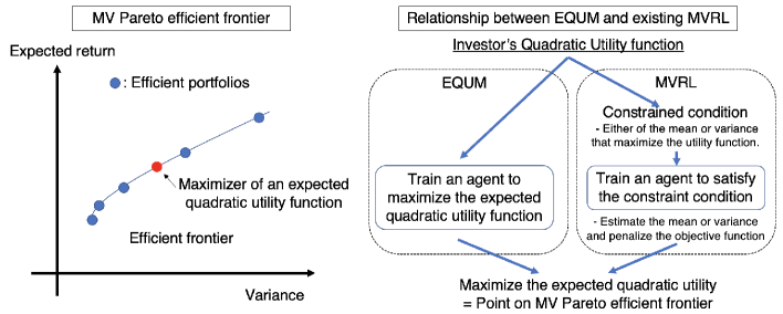
Figure 1: The concept of MV Preto efficient frontier and difference between EQUM and existing MVRL approaches.

In conclusion, we list the following three advantages to the EQUM approach:

(i)

the EQUM approach does not suffer from the double sampling issue by avoiding explicit approximation of the variance (Section 4);

(ii)

the EQUM approach is able to learn Pareto efficient policies and has plenty of interpretations from various perspectives (Section 4.3);

(iii)

we experimentally show that the EQUM approach returns more Pareto efficient policies than existing MVRL methods (Section 5).

Organization of this paper.

In the following sections, we first formulate the problem setting in Section 2 and review the existing methods in Section 3. Then, we propose the main algorithms in Section 4. Finally, we investigate the empirical effectiveness of the EQUM in Section 5.

2 Problem setting

We consider a standard setting of RL, where an agent interacts with an unfamiliar, dynamic, and stochastic environment modeled by a Markov decision process (MDP) in discrete time. We define an MDP as a tuple $(\mathcal{S},\mathcal{A},r,P,P_{0})$, where $\mathcal{S}$ is a set of states, $\mathcal{A}$ is a set of actions, $r:\mathcal{S}\times\mathcal{A}\to\mathbb{R}$ is a reward function, $P:\mathcal{S}\times\mathcal{S}\times\mathcal{A}\to[0,1]$ is a transition kernel, and $P_{0}:\mathcal{S}\to[0,1]$ is an initial state distribution. The initial state $\mathcal{S}_{1}$ is sampled from $P_{0}$. Let $\pi_{\theta}:\mathcal{A}\times\mathcal{S}\to[0,1]$ be a parameterized stochastic policy mapping states to actions, where $\theta$ is a tunable parameter. At time step $t$, an agent chooses an action $A_{t}$ following a policy $\pi_{\theta}(\cdot\mid S_{t})$. We assume that the policy $\pi_{\theta}$ is differentiable with respect to $\theta$; that is, $\frac{\partial\pi_{\theta}(s\mid a)}{\partial\theta}$ exists.

Let us define the expected cumulative reward from time step $t$ to $u$ as $\mathbb{E}_{\pi_{\theta}}[R_{t:u}]$, where $R_{t:u}=\sum^{u-t}_{i=0}\gamma^{i}r(S_{t+i},A_{t+i})$, $\gamma\in(0,1]$ is a discount factor and $\mathbb{E}_{\pi_{\theta}}$ denotes the expectation operator over a policy $\pi_{\theta}$, and $S_{1}$ is generated from $P_{0}$. When $\gamma=1$, to ensure that the cumulative reward is well-defined, we usually assume that all policies are proper (Bertsekas & Tsitsiklis, 1995); that is, for any policy $\pi_{\theta}$, an agent goes to a recurrent state $S^{*}$ with probability $1$, and obtains $0$ reward after passing the recurrent state $S^{*}$ at a stopping time $\tau$. This finite horizon setting is called episodic MDPs (Puterman, 1994). For brevity, we denote $R_{t:u}$ as $R$ when there is no ambiguity.

MV efficient policy.

Next, we introduce the goal of our problem. While a standard goal of RL is to maximize the expected cumulative reward $\mathbb{E}_{\pi_{\theta}}[R_{t:u}]$, risk-averse agents in various real-world applications also concern the uncertainty of the outcome. This paper represents the risk by the trajectory-variance $\mathrm{Var}_{\pi_{\theta}}(R_{t:u})$ and considers a situation where we incur a higher variance to achieve a higher expected cumulative reward. The goal of this paper is to control the trade-off between the expected cumulative reward (mean) and the trajectory-variance. To accomplish this purpose, we consider obtaining a policy located on MV efficient frontier, where we cannot increase the mean without increasing the variance or decrease the variance without decreasing the mean, under certain levels of the mean and variance that we want to achieve.

A typical approach to MV control involves solving a constrained problem, where we maximize the expected cumulative reward under a constraint of the trajectory-variance, or minimize the variance under a constraint of the expected cumulative reward. However, as we explain in the following sections, those MVRL methods suffer from a computational issue, called the double sampling issue. Therefore, this paper considers avoiding the double sampling issue by using the expected quadratic utility function as an alternative objective function. Its maximizer is located on the MV efficient frontier.

3 MVRL methods based on constraint problems

In this section, we review existing MVRL methods that attempt to solve a constraint problem.

3.1 Constrained trajectory-variance problem

Tamar et al. (2012), Prashanth & Ghavamzadeh (2013), and Xie et al. (2018) formulated MVRL by a constrained optimization problem defined as

$$\max_{\theta\in\Theta}\ \mathbb{E}_{\pi_{\theta}}[R]\ \ \ \mathrm{s.t.}\ \mathrm{Var}_{\pi_{\theta}}(R)=\eta.$$

In the MVRL formulation, the goal is to maximize the expected cumulative reward, while controlling the trajectory-variance at a certain level. To be more precise, their actual constraint condition is $\mathrm{Var}_{\pi_{\theta}}(R)\leq\eta$. However, if $\mathrm{Var}_{\pi_{\theta}}(R)=\eta$ is feasible, the optimizer satisfies the equality in a standard portfolio management setting. Therefore, we also only consider an equality constraint. To solve the problem, Tamar et al. (2012), Prashanth & Ghavamzadeh (2013), and Xie et al. (2018) considered a penalized method defined as $\max_{\theta\in\Theta}\mathbb{E}_{\pi_{\theta}}[R]-\delta g\big{(}\mathrm{Var}_{\pi_{\theta}}(R)-\eta\big{)}$, where $\delta>0$ is a constant and $g:\mathbb{R}\to\mathbb{R}$ is a penalty function, such as $g(x)=x$ or $g(x)=x^{2}$.

3.2 Double sampling issue

Tamar et al. (2012) and Prashanth & Ghavamzadeh (2013) reported the double sampling issue in MVRL, which requires sampling from two different trajectories to estimate the policy gradient. For instance, in an episodic MDP with the discount factor $\gamma=1$ and the stopping time $\tau=\min\{t\mid S_{t}=S^{*}\}$, the gradients of $\mathbb{E}_{\pi_{\theta}}[R]$, $\mathbb{E}_{\pi_{\theta}}\big{[}R^{2}\big{]}$, and $\big{(}\mathbb{E}_{\pi_{\theta}}[R]\big{)}^{2}$ are given as follows (Tamar et al., 2012):

$$\nabla_{\theta}\mathbb{E}_{\pi_{\theta}}[R]=\mathbb{E}_{\pi_{\theta}}\left[R\sum^{\tau}_{t=1}\nabla_{\theta}\log\pi_{\theta}(S_{t},A_{t})\right],\ \ \ \nabla_{\theta}\mathbb{E}_{\pi_{\theta}}\big{[}R^{2}\big{]}=\mathbb{E}\left[R^{2}\sum^{\tau}_{t=1}\nabla_{\theta}\log\pi_{\theta}(S_{t},A_{t})\right],$$

$$\nabla_{\theta}\big{(}\mathbb{E}_{\pi_{\theta}}[R]\big{)}^{2}=2\mathbb{E}_{\pi_{\theta}}[R]\nabla_{\theta}\mathbb{E}_{\pi_{\theta}}[R].$$

Besides, the gradient of the variance is given as $\mathbb{E}_{\pi_{\theta}}\left[R^{2}\sum^{\tau}_{t=1}\nabla_{\theta}\log\pi_{\theta}(S_{t},A_{t})\right]-2\mathbb{E}_{\pi_{\theta}}[R]\nabla_{\theta}\mathbb{E}_{\pi_{\theta}}[R]$. Because optimizing the policy $\pi_{\theta}$ directly using the gradients is computationally intractable, we replace them with their unbiased estimators. Suppose that there is a simulator generating a trajectory $k$ with $\{(S^{k}_{t},A^{k}_{t},r(S^{k}_{t},A^{k}_{t}))\}^{\tau^{k}}_{t=1}$, where $\tau^{k}$ is the stopping time of the trajectory. Then, we can construct unbiased estimators of $\mathbb{E}_{\pi_{\theta}}[R]$ and $\mathbb{E}_{\pi_{\theta}}\big{[}R^{2}\big{]}$ as follows (Tamar et al., 2012):

$$\widehat{\nabla}_{\theta}\mathbb{E}_{\pi_{\theta}}[R]=\widehat{R}^{k}\sum^{\tau^{k}}_{t=1}\nabla_{\theta}\log\pi_{\theta}(S^{k}_{t},A^{k}_{t})\ \mathrm{and}\ \widehat{\nabla}_{\theta}\mathbb{E}_{\pi_{\theta}}\big{[}R^{2}\big{]}=\left(\widehat{R}^{k}\right)^{2}\sum^{\tau^{k}}_{t=1}\nabla_{\theta}\log\pi_{\theta}(S^{k}_{t},A^{k}_{t}),$$ (1)

where $\widehat{R}^{k}$ is a sample approximation of $\mathbb{E}_{\pi_{\theta}}[R]$ at the episode $k$. However, obtaining an unbiased estimator of $\nabla_{\theta}\big{(}\mathbb{E}_{\pi_{\theta}}[R]\big{)}^{2}=2\mathbb{E}_{\pi_{\theta}}[R]\nabla_{\theta}\mathbb{E}_{\pi_{\theta}}[R]$ is difficult because it requires sampling from two different trajectories for approximating $\mathbb{E}_{\pi_{\theta}}[R]$ and $\nabla_{\theta}\mathbb{E}_{\pi_{\theta}}[R]$. This issue makes the optimization problem difficult.

3.3 Existing approaches

For the double sampling issue, Tamar et al. (2012), Prashanth & Ghavamzadeh (2013, 2016), and Xie et al. (2018) presented the following solutions.

Multi-time-scale stochastic optimization.

Tamar et al. (2012) and Prashanth & Ghavamzadeh (2013, 2016) proposed finding an equilibrium point of an ordinary differential equation and a saddle point of the penalized optimization problem, respectively, by using multi-time-scale stochastic optimization.

Coordinate descent optimization.

Xie et al. (2018) proposed using the Legendre-Fenchel dual transformation with coordinate descent algorithm. First, based on Lagrangian relaxation, Xie et al. (2018) set an objective function as $\max_{\theta\in\Theta}\mathbb{E}_{\pi_{\theta}}[R]-\delta\left(\mathrm{Var}_{\pi_{\theta}}(R)-\eta\right)$. Then, Xie et al. (2018) transformed the objective function as $\max_{\theta\in\Theta,y\in\mathbb{R}}2y\left(\mathbb{E}_{\pi_{\theta}}[R]+\frac{1}{2\delta}\right)-y^{2}-\mathbb{E}_{\pi_{\theta}}\left[R^{2}\right]$ and trained an agent by solving the optimization problem via a coordinate descent algorithm.

Weakness of existing approaches.

Multi-time-scale approaches proposed by Tamar et al. (2012) and Prashanth & Ghavamzadeh (2013, 2016) are known to be sensitive to the choice of step-size schedules, which are not easy to control (Xie et al., 2018). The method proposed by Xie et al. (2018) does not reflect the constraint condition $\eta$; that is, in the objective function of Xie et al. (2018), there exists a penalty coefficient $\delta$, but there is no constraint condition $\eta$. The problem of Xie et al. (2018) is caused by their objective function based on the penalty function $g(x)=x$: $\mathbb{E}_{\pi_{\theta}}[R]-\delta\left(\mathrm{Var}_{\pi_{\theta}}(R)-\eta\right)$, where the first derivative does not include $\eta$. In standard Lagrange relaxation, we also need to use an iterative algorithm to decide an optimal $\delta$. However, it does not seem easy to add the procedure to the method of Xie et al. (2018). In addition, when using quadratic function $g(x)=x^{2}$ as the penalty, we cannot remove $(\mathbb{E}[R])^{2}$ even with Legendre-Fenchel dual; that is, the method still suffers from the double sampling issue.

4 EQUM for MV efficient RL

For MVRL by an efficient policy, we propose direct EQUM with a policy gradient method. In social sciences, we often assume that an agent maximizes the expected quadratic utility function. This utility function is often used in financial theory. Based on this classical result, we motivate our proposed method, EQUM, for obtaining an MV efficient policy.

4.1 Quadratic utility function and MV trade-off

For a cumulative reward $R$, we define the quadratic utility function as $u(R;\alpha,\beta)=\alpha R-\frac{1}{2}\beta R^{2}$, where $\alpha>0$ and $\beta\geq 0$. We consider learning a policy that maximizes the expected value of this quadratic utility function. The expected quadratic utility function $\mathbb{E}_{\pi_{\theta}}\left[u(R;\alpha,\beta)\right]$ is known to be Pareto efficient in the sense of mean and variance when its optimal value satisfies $\mathbb{E}_{\pi}[R]\leq\frac{\alpha}{\beta}$. In order to confirm this, we can decompose the expected quadratic utility as

$$\mathbb{E}_{\pi_{\theta}}\left[u(R;\alpha,\beta)\right]=-\frac{1}{2}\beta\left(\mathbb{E}_{\pi_{\theta}}[R]-\frac{\alpha}{\beta}\right)^{2}+\frac{\alpha^{2}}{2\beta}-\frac{1}{2}\beta\mathrm{Var}_{\pi_{\theta}}(R).$$ (2)

When a policy maximizes the expected quadratic utility with respect to all feasible policies, it is equivalent to an MV portfolio (Borch, 1969; Baron, 1977; Luenberger et al., 1997). Following (Luenberger et al., 1997, p.237–239), we explain this as follows:

1. Among policies $\pi_{\theta}$ with a fixed mean $\mathbb{E}_{\pi}[R]=\mu$, the policy with the lowest variance maximizes the expected quadratic utility function because $\mathbb{E}_{\pi_{\theta}}\left[u(R;\alpha,\beta)\right]=\alpha\mu-\frac{1}{2}\beta\mu^{2}-\frac{1}{2}\beta\mathrm{Var}_{\pi_{\theta}}(R)$ is a monotonous decreasing function on $\mathrm{Var}_{\pi_{\theta}}(R)$;

2. Among policies $\pi_{\theta}$ with a fixed variance $\mathrm{Var}_{\pi_{\theta}}(R)=\sigma^{2}$ and mean $\mathbb{E}_{\pi}[R]\leq\frac{\alpha}{\beta}$, the policy with the highest mean maximizes the expected quadratic utility function because $\mathbb{E}_{\pi_{\theta}}\left[u(R;\alpha,\beta)\right]=-\frac{1}{2}\beta\left(\mathbb{E}_{\pi_{\theta}}[R]-\frac{\alpha}{\beta}\right)^{2}+\frac{\alpha^{2}}{2\beta}-\frac{1}{2}\beta\sigma^{2}$ is a monotonous increasing function on $\mathbb{E}_{\pi_{\theta}}[R]\leq\frac{\alpha}{\beta}$.

4.2 EQUM

Based on the above property, we propose maximizing the expected quadratic utility function in RL; that is, training an agent to directly maximize the expected quadratic utility function for MV control instead of solving a constrained optimization. We call the framework that makes the RL objective function an expected quadratic utility EQUM.

Here, we present two advantages of RL for EQUM. The first advantage concerns computation. In EQUM, we do not suffer from the double sampling issue because the term $\left(\mathbb{E}_{\pi_{\theta}}[R]\right)^{2}$, which causes the problem, is absent, and we must only estimate the gradients of $\mathbb{E}_{\pi_{\theta}}\left[R\right]$ and $\mathbb{E}_{\pi_{\theta}}\left[R^{2}\right]$. The second advantage is that it provides a variety of interpretations, as listed in Section 4.3.

EQUM is an agnostic in learning method. As an example, we show an implementation based on a simple policy gradient method.

Policy Gradient for EQUM.

We introduce a main algorithm for EQUM with a simple policy gradient method (Brockman et al., 2016; Williams, 1992). For an episode $k$ with the length $n$, the proposed algorithm replaces $\mathbb{E}_{\pi_{\theta}}\big{[}R\big{]}$ and $\mathbb{E}_{\pi_{\theta}}\big{[}R^{2}\big{]}$ with the sample approximations $\sum^{n}_{t=1}\gamma^{t-1}r(S_{t},A_{t})$ and $\left(\sum^{n}_{t=1}\gamma^{t-1}r(S_{t},A_{t})\right)^{2}$, respectively (Tamar et al., 2012); that is, the unbiased gradients are given as (1). Therefore, for a sample approximation $\widehat{R}^{k}$ of $\mathbb{E}_{\pi_{\theta}}\big{[}R^{2}\big{]}$ at the episode $k$, we optimize the policy with ascending the unbiased gradient $\left(\alpha\widehat{R}^{k}-\frac{1}{2}\beta\left(\widehat{R}^{k}\right)^{2}\right)\sum^{n}_{t=1}\nabla_{\theta}\log\pi_{\theta}(S^{k}_{t},A^{k}_{t})$. We also introduce the actor-critic-based method in Appendix E.

4.3 Interpretations of EQUM

We can interpret EQUM as an approach for (i) a targeting optimization problem to achieve an expected cumulative reward $\zeta$, (ii) an expected cumulative reward maximization with regularization, and (iii) expected utility maximization via Taylor approximation.

First, we can also interpret EQUM as mean squared error (MSE) minimization between a cumulative reward $R$ and a target return $\zeta$; that is,

$$\operatorname*{arg\,min}_{\theta\in\Theta}J(\theta;\zeta)=\operatorname*{arg\,min}_{\theta\in\Theta}\mathbb{E}_{\pi_{\theta}}\left[\big{(}\zeta-R\big{)}^{2}\right]$$ (3)

We can decompose the MSE into the bias and variance as

$$\mathbb{E}_{\pi_{\theta}}\left[\big{(}\zeta-R\big{)}^{2}\right] =\underbrace{\big{(}\zeta-\mathbb{E}_{\pi_{\theta}}[R]\big{)}^{2}}_{\text{Bias}}+\underbrace{2\mathbb{E}_{\pi_{\theta}}\Big{[}\big{(}\zeta-\mathbb{E}_{\pi_{\theta}}[R]\big{)}\big{(}\mathbb{E}_{\pi_{\theta}}[R]-R\big{)}\Big{]}}_{\text{0}}+\underbrace{\mathbb{E}_{\pi_{\theta}}\left[\big{(}\mathbb{E}_{\pi_{\theta}}[R]-R\big{)}^{2}\right]}_{\text{Variance}}$$

$$=\zeta^{2}-2\zeta\mathbb{E}_{\pi_{\theta}}[R]+\big{(}\mathbb{E}_{\pi_{\theta}}[R]\big{)}^{2}+\mathbb{E}_{\pi_{\theta}}\left[\big{(}\mathbb{E}_{\pi_{\theta}}[R]-R\big{)}^{2}\right].$$

Thus, the MSE minimization (3) is equivalent to EQUM (2), where $\zeta=\frac{\alpha}{\beta}$. The above equation provides an important implication for the setting of $\zeta$. If we know the reward is shifted by $x$, we only have to adjust $\zeta$ to $\zeta+x$. This is because $\zeta$ only affects the bias term in the above equation. The equation also provides another insight. If our assumption $\max_{\pi_{\theta}}\mathbb{E}_{\pi_{\theta}}[R]\leq\zeta$ is violated, $\mathbb{E}_{\pi_{\theta}}[R]$ will not be maximized with a fixed variance and will be biased towards $\zeta$. That is, in that case, EQUM cannot find the MV efficient policies. In applications, we can confirm whether the optimization works by checking whether average value of the empirically realized cumulative rewards is less than $\zeta$.

Second, we can regard the quadratic utility function as an expected cumulative reward maximization with a regularization term defined as $\mathbb{E}\big{[}R^{2}\big{]}$; that is, minimization of the risk $\mathcal{R}(\pi_{\theta})$:

$$\mathcal{R}(\theta)=\underbrace{-\mathbb{E}_{\pi_{\theta}}[R]}_{\text{Risk of expected cumulative reward maximization}}+\underbrace{\psi\mathbb{E}_{\pi_{\theta}}\big{[}R^{2}\big{]}}_{\text{Regularization term}}$$

where $\psi>0$ is a regulation parameter and $\psi=\frac{\beta}{2\alpha}=\frac{1}{2\zeta}$. As $\zeta\to\infty$, $\mathcal{R}(\pi_{\theta})\to-\mathbb{E}_{\pi_{\theta}}[R]$.

Third, the quadratic utility function is the quadratic Taylor approximation of a smooth utility function $u(R)$ because for $R_{0}\in\mathbb{R}$, we can expand it as $u(R)\approx u(R_{0})+U^{\prime}(R_{0})(R-R_{0})+U^{\prime\prime}(R_{0})(R-R_{0})^{2}+\cdots$; that is, quadratic utility is an approximation of various risk-averse utility functions. This property also supports the use of the quadratic utility function in practice.

It should be noted that the EQUM is closely related to the fields of economics and finance, where the ultimate goal is to maximize the utility of an agent, which is also referred to as an investor. The quadratic utility function is a standard risk-averse utility function often assumed in financial theory Luenberger et al. (1997) to justify an MV portfolio; that is, an MV portfolio maximizes an investor’s utility function if the utility function is quadratic (see Appendix A). Therefore, our approach can be interpreted as a method that directly achieves the original goal (Figure 1).

4.4 Specification of utility function

Next, we discuss how to decide the parameters $\alpha$ and $\beta$, which are equivalent to $\zeta$, $\xi$, and $\psi$. The meanings are equivalent to constrained conditions of MVRL; that is, we predetermine these hyperparameters depending on our attitude toward risk. For instance, we propose the following three directions for the parameter choice. First, we can determine $\frac{\beta}{2\alpha}=\psi$ based on economic theory or market research (Ziemba et al., 1974; Kallberg et al., 1983) (Appendix A). Luenberger et al. (1997) proposed some questionnaires to investors for the specification. Second, we set $\zeta=\frac{1}{2\psi}$ as the targeted reward that investors aim to achieve. Third, through cross-validation, we can optimize the regularization parameter $\psi$ to maximize some criteria, such as the Sharpe ratio (Sharpe, 1966).

However, we note that in time-series related tasks, we cannot use standard cross-validation owing to dependency. Therefore, in our experiments of portfolio analysis with a real-world financial dataset, we show various results under different parameters.

4.5 Differences from conventional MVRL

Readers may assert that EQUM simply omits $\left(\mathbb{E}_{\pi_{\theta}}[R]\right)^{2}$ from a standard MVRL and is the essentially the same. However, they are significantly different; one of the main findings of this paper is our formulation of a simpler RL problem to obtain an MV efficient policy. Existing MVRL methods suffer from computational difficulties caused by the double sampling issue. However, we can obtain MV efficient policy without going through the difficult problem. In addition, EQUM shows better performance in experiments even from the viewpoint of the constrained problem because it is difficult to choose parameters to avoid the double sampling issue in existing approaches. Therefore, this paper recommends the use of EQUM to avoid solving more difficult constrained problems to achieve MV control. Note that between MV portfolio and EQUM, the essential meanings of the hyperparameters are the same; that is, the constrained conditions of the MVRL are determined by the utility function of the agent. In economic and financeial applications, EQUM is directly related to the motivation, which is not to solve the constrained problem, but to maximize the expected utility.

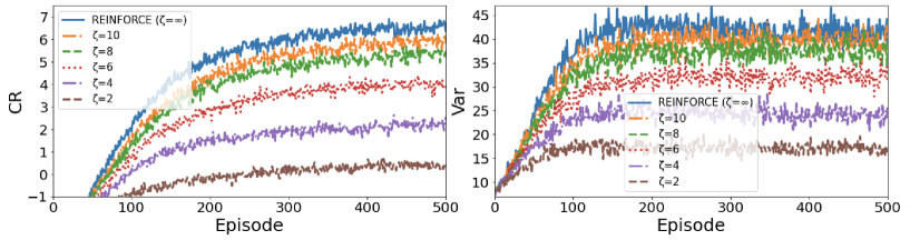
Figure 2: The CRs and Vars in the training process of the experiment using the synthetic dataset.

5 Experimental studies

This section investigates the empirical performance of the proposed EQUM with policy gradient (EQUM) using synthetic and real-world financial datasets. We conduct two experiments. In the first experiments, following Tamar et al. (2012), Tamar et al. (2014), and Xie et al. (2018), we conduct portfolio management experiments with synthetic datasets. In the third experiment, we conduct a portfolio management experiment with a dataset of Fama & French (1992), a standard benchmark in finance. In Appendix C, following Tamar et al. (2012), Tamar et al. (2014), and Xie et al. (2018), we also conduct American-style option experiments with synthetic datasets. We implemented algorithms following the Pytorch example. For algorithms using neural networks, we use a three layer perceptron, where the numbers of the units in two hidden layers are the same as that of the input node, and that of the output node is $2$. We note that in all results, naively maximizing the reward or minimizing the variance do not ensure a better algorithm; we evaluate an algorithm based on how it controls the MV trade-off. We denote the hyperparameter of the EQUM by $\zeta$, which has the same meaning as $(\alpha,\beta)$ and $\psi$. For all experiments, we adopt episodic MDPs; that is, $\gamma=1$.

5.1 Portfolio management with a synthetic dataset

Following Tamar et al. (2012) and Xie et al. (2018), we consider a portfolio composed of two types of assets: a liquid asset, which has a fixed interest rate $r_{\mathrm{l}}$, and a non-liquid asset, which has a time-dependent interest rate taking either $r^{\mathrm{low}}_{\mathrm{nl}}$ or $r^{\mathrm{high}}_{\mathrm{nl}}$, and the transition follows a switching probability $p_{\mathrm{switch}}$. We can sell the liquid asset at every time step $t=1,2,\dots,T$ but the non-liquid asset can only be sold after the maturity $W$ periods. This means that when holding $1$ liquid asset, we obtain $r_{\mathrm{l}}$ per period; when holding $1$ non-liquid asset at the $t$-th period, we obtain $r^{\mathrm{low}}_{\mathrm{nl}}$ or $r^{\mathrm{high}}_{\mathrm{nl}}$ at the $t+W$-th period. In addition, the non-liquid asset has a risk of not being paid with a probability $p_{\mathrm{risk}}$; that is, if the non-liquid asset defaulted during the $W$ periods, we could not obtain any rewards by having the asset. In this setup, a typical investment strategy is to construct a portfolio using both liquid and non-liquid assets for MV control. In our model, an investor can change the portfolio by investing a fixed fraction $w$ of the total capital $M$ in the non-liquid asset at each time step. Following Xie et al. (2018), we set $r_{\mathrm{l}}=1.001$, $r^{\mathrm{low}}_{\mathrm{nl}}=1.1$, $r^{\mathrm{high}}_{\mathrm{nl}}=2$, $p_{\mathrm{switch}}=0.1$, $p_{\mathrm{risk}}=0.05$, $W=4$, $w=0.2$, and $M=1$. As a performance metric, we use the average cumulative reward (CR) and its variance (Var) when investing for $50$ periods. We compare the EQUM with the REINFORCE, a policy gradient for solving a variance-constrained optimization by Tamar et al. (2012) (Tamar), and a coordinate descent-based algorithm by Xie et al. (2018) (Xie). We denote the variance constraint of Tamar et al. (2012) as $\mathrm{var}$ and Lagrange multiplier of Xie et al. (2018) as $\lambda$. For optimizing Tamar, Xie, and EQUM, we set the Adam optimizer with learning rate $0.01$ and weight decay parameter $0.1$. For each algorithm, we report performances under various hyperparameters as much as possible.

First, we show CRs and Vars of the EQUM during the training process in Figure 2, where we conduct $100$ trials on the test environment to compute CRs and Vars for each episode. Here, we also show the performance of REINFORCE, which corresponds to the EQUM with $\zeta=\alpha/\beta=\infty$. As Figure 2 shows, the EQUM trains MV controlled portfolios well depending on the parameter $\zeta$. Next, we compare the performances of the EQUM on the test environment with those of the REINFORCE, Tamar, and Xie. We conduct $100,000$ trials on the test environment to compute CRs and Vars.

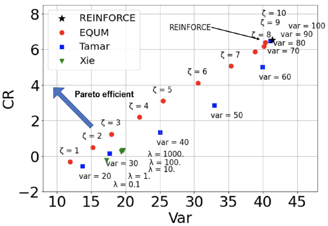
Figure 3: MV efficiency of the portfolio management experiment. Higher CRs and lower Vars methods are MV Pareto efficient.

In Figure 3, we plot performances under several hyperparameters on a test environment, where the horizontal axis denotes the Var, and the vertical axis denotes the CR. Trained agents with a higher CR and lower Var are Pareto efficient. As the result shows, the EQUM returns more efficient portfolios than the other algorithms in almost all cases. We conjecture that this is because while the EQUM is an end-to-end optimization for obtaining an efficient agent, the other methods consist of two steps of estimating the variance and solving the constrained optimization, where the estimation error of the variance is a source of the suboptimal result. We show CRs and Vars of some of their results in the upper table of Table 1. We also denote MSE between $\zeta$ and CR in the lower table of 1. From the table, we can confirm that the EQUM succeeded in minimizing the MSEs.

Table 1: The results of the portfolio management with a synthetic data. The upper table shows the CRs and Vars over $100,000$ trials. The lower table shows the MSEs for $\zeta$ over $100,000$ trials.

	REINFORCE	EQUM			Tamar		Xie
	($\zeta=\infty$)	$\zeta=10$	$\zeta=6$	$\zeta=4$	$\mathrm{var}=80$	$\mathrm{var}=50$	$\lambda=100$	$\lambda=10$
CR	6.729	6.394	4.106	2.189	6.709	2.851	0.316	0.333
Var	32.551	31.210	24.424	18.518	32.586	21.573	15.883	15.992

	REINFORCE	EQUM
Target Value	($\zeta=\infty$)	$\zeta=10$	$\zeta=8$	$\zeta=6$	$\zeta=4$	$\zeta=2$
MSE from $\zeta=10$	51.669	53.399	55.890	65.307	83.061	105.492
$\zeta=8$	42.586	42.975	43.375	45.730	55.816	71.480
$\zeta=6$	41.503	40.551	38.860	34.154	36.570	45.467
$\zeta=4$	48.420	46.127	42.345	30.577	25.324	27.455
$\zeta=2$	63.337	59.703	53.830	35.000	22.078	17.442

5.2 Portfolio management with a real-world dataset

We use well-known benchmarks called Fama & French (FF) datasets to ensure the reproducibility of the experiment Fama & French (1992). Among FF datasets, we use the FF25, FF48 and FF100 datasets, where the FF25 and FF 100 dataset includes $25$ and $100$ assets formed based on size and book-to-market ratio; the FF48 dataset contains $48$ assets representing different industrial sectors. We use all datasets covering monthly data from July 1980 to June 2020. We formulate the problem with an episodic MDP. The state is the past $12$ months of returns of each asset and the action is defined as portfolio weight; that is, the number of actions is equal to that of assets. The reward is obtained as the portfolio return. Here, the portfolio return at time $1\leq t\leq T$ is defined as $y_{t}=\sum_{j=1}^{m}y_{j,t}w_{j,t-1}$, where $y_{j,t}$ is the return of $j$ asset at time $t$, $w_{j,t-1}$ is the weight of $j$ asset in the portfolio at time $t-1$, and $m$ is the number of assets. We optimize the weight to obtain a portfolio return controlling for MV trade-off. The length of the episode is $1$ years ($12$ months). For the stochastic policy, we adopt a three-layer feed-forward neural network with the ReLU activation function where the number of units in each respective layer is equal to the number of assets, $100$, $50$, and the number of assets. We use the softmax function for the output layer, which determines the weight $w_{j,t-1}$.

Table 2: The performance of each portfolio model during the out-of-sample period (from July 2000 to June 2020) for FF25 dataset (upper table) , FF48 (middle table), and FF100 (lower table). For each dataset, the best performance is highlighted in bold.

Method	EW	MV	EGO	BLD	Tamar			Xie			EQUM
					$\mathrm{var}=2.5$	$\mathrm{var}=5$	$\mathrm{var}=10$	$\lambda=10$	$\lambda=100$	$\lambda=1000$	$\zeta=0.5$	$\zeta=0.75$	$\zeta=1.5$
FF25
CR$\uparrow$	0.80	0.11	0.87	0.56	0.96	1.19	1.20	0.90	0.90	1.02	1.02	0.81	1.25
Var$\downarrow$	28.62	53.58	30.63	12.01	48.86	34.03	34.01	30.99	30.99	16.25	18.63	12.39	15.02
R/R$\uparrow$	0.52	0.05	0.55	0.56	0.48	0.71	0.71	0.56	0.56	0.87	0.82	0.80	1.12
MaxDD$\downarrow$	0.54	0.75	0.57	0.37	0.64	0.58	0.58	0.57	0.57	0.30	0.36	0.30	0.31
FF48
CR$\uparrow$	0.81	0.15	1.04	0.52	0.50	0.78	0.63	1.44	1.39	0.88	0.99	1.03	0.94
Var$\downarrow$	22.91	76.89	31.87	9.65	14.52	18.66	18.08	47.90	39.87	34.17	11.50	19.72	32.70
R/R$\uparrow$	0.59	0.06	0.64	0.58	0.46	0.63	0.51	0.72	0.76	0.52	1.01	0.80	0.57
MaxDD$\downarrow$	0.53	0.84	0.53	0.38	0.58	0.54	0.45	0.56	0.52	0.65	0.29	0.45	0.45
FF100
CR$\uparrow$	0.81	0.14	0.86	0.53	1.31	0.99	1.13	1.23	0.95	1.33	1.36	0.95	1.09
Var$\downarrow$	29.36	57.90	32.40	11.79	32.67	17.17	33.62	43.67	81.98	43.65	20.05	15.50	14.81
R/R$\uparrow$	0.52	0.06	0.53	0.54	0.79	0.83	0.68	0.64	0.36	0.70	1.05	0.83	0.98
MaxDD$\downarrow$	0.55	0.72	0.58	0.36	0.39	0.49	0.38	0.52	0.65	0.46	0.39	0.31	0.24

Portfolio models.

We use the following portfolio models. An equally-weighted portfolio (EW) weights the financial assets equally (DeMiguel et al., 2009). A mean-variance portfolio (MV) computes the optimal variance under a mean constraint (Markowitz, 1952). To compute the mean vector and covariance matrix, we use the latest $10$ years ($120$ months) data. A Kelly growth optimal portfolio with ensemble learning (EGO) is proposed by Shen et al. (2019). We set the number of resamples as $m_{1}=50$, the size of each resample $m_{2}=5\tau$, the number of periods of return data $\tau=60$, the number of resampled subsets $m_{3}=50$, and the size of each subset $m_{4}=n^{0.7}$, where $m$ is number of assets; that is, $m=25$ in FF25, $m=48$ in FF48 and $m=100$ in FF100. Portfolio blending via Thompson sampling (BLD) is proposed by Shen & Wang (2016). We use the latest $10$ years ($120$ months) data to compute for the sample covariance matrix and blending parameters. A policy gradient with variance-related risk criteria (Tamar) is proposed by Tamar et al. (2012). We set the target variance terms var from $\{2.5,5,10\}$. The block coordinate ascent algorithm is proposed by Xie et al. (2018) (Xie). We set the regularization parameters $\lambda$ from $\{10,100,1000\}$. Then, let us denote the EQUM with the policy gradient as EQUM. The parameter $\zeta$ is chosen from $\{0.5,0.75,1.5\}$. For optimizing Tamar, Xie and EQUM, we use the Adam optimizer with learning rate $0.01$ and weight decay parameter $0.1$. We train the neural networks for $10$ episodes. Each portfolio is updated by sliding one-month-ahead.

Performance metrics.

The following measures widely used in finance to evaluate portfolio strategies (Brandt, 2010) are chosen. The cumulative reward (CR), annualized risk as the standard deviation of return (RISK) and risk-adjusted return (R/R) are defined as follows: $\mathrm{CR}=1/T\sum_{t=1}^{T}y_{t}$, $\mathrm{Var}=1/T\sum_{t=1}^{T}(y_{t}-\mathrm{CR})^{2}$, and $\mathrm{R/R}=\sqrt{12}\times\mathrm{CR}/\sqrt{\mathrm{Var}}$. R/R is the most important measure for a portfolio strategy and is often referred to as the Sharpe Ratio (Sharpe, 1966). We also evaluate the maximum draw-down (MaxDD), which is another widely used risk measure (Magdon-Ismail & Atiya, 2004) for the portfolio strategy. In particular, MaxDD is the largest drop from a peak defined as $\mathrm{MaxDD}=\min_{t\in[1,T]}\left(0,\frac{W_{t}}{\max_{\tau\in[1,t]}W_{\tau}}-1\right)$, where $W_{k}$ is the cumulative return of the portfolio until time $k$; that is, $W_{t}=\prod_{t^{\prime}=1}^{t}(1+y_{t^{\prime}})$.

Table 2 reports the performances of the portfolios. In almost all cases, the EQUM portfolio achieves the highest R/R and the lowest MaxDD. Therefore, we can confirm that the EQUM portfolio has a high R/R, and avoids a large drawdown. The real objective (minimizing variance with a penalty on return targeting) for Tamar, MVP, and EQUM is shown in Appendix D. Except for FF48’s MVP, the objective itself is smaller than that of EQUM. Since the values of the objective are proportional to R/R, we can empirically confirm that the better optimization, the better performance.

6 Conclusion

In this paper, we proposed EQUM for MV controlled RL. Compared with the conventional MVRL methods, EQUM is computationally friendly. The proposed EQUM framework also includes various interpretations, such as targeting optimization and regularization, which expands the scope of applications of the method. We investigated the effectiveness of the EQUM framework compared with the standard RL and existing MVRL methods through experiments using synthetic and real-world datasets. The proposed method successfully controlled the MV trade-off and returned more MV Pareto efficient policies.

Our proposed method is expected to be applied especially in finance, we need to carefully consider the model of cumulative rewards considering the time-series nature to prevent fatal failures in trading. In addition, the application of machine learning methods may result in unintended consequences such as market manipulation, and care should be taken to follow the market rules.

Appendix A Preliminaries of economic and financial theory

A.1 Utility theory

Utility theory is the foundation of the choice theory under uncertainty including economics and financial theory. A utility function $u(\cdot)$ measures agent’s relative preference for different levels of total wealth $W$. According to Morgenstern & Von Neumann (1953), a rational agent makes an investment decision to maximize the expected utility of wealth among a set of competing feasible investment alternatives. For simplicity, the following assumptions are often made for the utility function used in economics and finance. First, the utility function is assumed to be at least twice continuous differentiable. The first derivative of the utility function (the marginal utility of wealth) is always positive, i.e., $U^{{}^{\prime}}(W)>0$, because of the assumption of non-satiation. The second assumption concerns risk attitude of the agents called “risk averse". When we assume that an agent is risk averse, the utility function is described as a curve that increases monotonically and is concave. The most often used utility function of a risk-averse agent is the quadratic utility function as follows:

$$u(W;\alpha,\beta)=\alpha W-\beta\frac{1}{2}W^{2}$$ (4)

where $\alpha\geq 0,\beta>0$. Taking the expected value of the quadratic utility function in (4) yields:

$$E[u(W;\alpha,\beta)]=\alpha\mathbb{E}[W]-\frac{1}{2}\beta\mathbb{E}[W^{2}]$$ (5)

Substituting $\mathbb{E}[W^{2}]=\mathrm{Var}[W]+\mathbb{E}[W]^{2}$ into (4) gives

$$\mathbb{E}[u(W;\alpha,\beta)]=\alpha\mathbb{E}[W]-\frac{1}{2}\beta(\mathrm{Var}[W]+\mathbb{E}[W]^{2})$$ (6)

Equation (6) shows that expected quadratic utility can be described in terms of mean $E[W]$ and variance $\mathrm{Var}[W]$ of wealth. Therefore, the assumption of a quadratic utility function is crucial to the mean-variance analysis.

Remark 1 (Approximation by quadratic utility function).

Readers may be interested in how the quadratic utility function approximates other risk averse utility functions. Kroll et al. (1984) empirically answered this question by comparing MV portfolio (maximizer of expected quadratic utility function) and maximizers of other utility functions. In their study, maximizers of other utility functions also almost located in MV Pareto efficient frontier; that is, expected quadratic utility function approximates other risk averse utility function well.

Remark 2 (Non-vNM utility functions).

Unlike MV trade-off, utility functions maximized by some recently proposed new risk criteria, such as VaR and Prospect theory, do not belong to traditional vNM utility function.

A.2 Markowitz’s portfolio

Considering the mean-variance trade-off in a portfolio and economic activity is an essential task in economics as Tamar et al. (2012) and Xie et al. (2018) pointed out. The mean-variance trade-off is justified by assuming either quadratic utility function to the economic agent or multivariate normal distribution to the financial asset returns (Borch, 1969; Baron, 1977; Luenberger et al., 1997). This means that if either the agent follows the quadratic utility function or asset return follows the normal distribution, the agent’s expected utility function is maximized by maximizing the expected reward and minimizing the variance. Therefore, the goal of Markowitz’s portfolio is not only to construct the portfolio itself but also to maximize the expected utility function of the agent.

Markowitz (1952) proposed the following steps for constructing a MV controlled portfolio (Also see Markowitz (1959), page 288, and Luenberger et al. (1997)):

• Constructing portfolios minimizing the variance under several reward constraint;

• Among the portfolios constructed in the first step, the economic agent chooses a portfolio maximizing the utility function.

Conventional financial methods often adopt this two-step approach because directly predicting the reward and variance to maximize the expected utility function is difficult; therefore, first gathering information based on analyses of an economist, then we construct the portfolio using the information and provide the set of the portfolios to an economic agent. However, owing to the recent development of machine learning, we can directly represent the complicated economic dynamics using flexible models, such as deep neural networks. In addition, as Tamar et al. (2012) and Xie et al. (2018) reported, when constructing the mean-variance portfolio in RL, we suffer from the double sampling issue. Therefore, this paper aims to achieve the original goal of the mean-variance approach; that is, the expected utility maximization. Note that this idea is not restricted to financial applications but can be applied to applications where the agent utility can be represented only by the mean and variance.

A.3 Markowitz’s portfolio and capital asset pricing model

Markowitz’s portfolio is known as the mean-variance portfolio (Markowitz, 1952; Markowitz & Todd, 2000). Constructing the mean-variance portfolio is motivated by the agent’s expected utility maximization. When the utility function is given as the quadratic utility function, or the financial asset returns follow the multivariate normal distribution, a portfolio maximizing the agent’s expected utility function is given as a portfolio with minimum variance under a certain standard expected reward.

The Capital Asset Pricing Model (CAPM) theory is a concept which is closely related to Markowitz’s portfolio (Sharpe, 1964; Lintner, 1965; Mossin, 1966). This theory theoretically explains the expected return of investors when the investor invests in a financial asset; that is, it derives the optimal price of the financial asset. To derive this theory, as well as Markowitz’s portfolio, we assume the quadratic utility function to the investors or the multivariate normal distribution to the financial assets.

Merton (1969) extended the static portfolio selection problem to a dynamic case. Fishburn & Burr Porter (1976) studied the sensitivity of the portfolio proportion when the safe and risky asset distributions change under the quadratic utility function. Thus, there are various studies investigating relationship between the utility function and risk-averse optimization (Tobin, 1958; Kroll et al., 1984; Bulmuş & Özekici, 2014; Bodnar et al., 2015a, b).

A.4 MV portfolio and MVRL

Traditional portfolio theory have attempted to maximize the expected quadratic utility function by providing MV portfolios. This is because MV portfolio is easier to interpret than EQUM, and we can obtain a solution by quadratic programming. One of the main goals of MVRL methods is also to construct MV portfolio under a dynamic environment (Tamar et al., 2012). However, we conjecture that there are three significant differences between them. First, unlike static problem, MVRL suffers computational difficulties. Second, while static problem solves quadratic programming given the expected reward and variance, MVRL methods simultaneously estimate these values and solve the constrained problem. Third, while static MV portfolios gives us an exact solution of the constrained problem, MVRL often relaxes the constrained problem by penalized method, which causes approximation errors. In particular, for the second and third points, the difference in how to handle the estimators of expected reward and variance is essential.

A.5 Empirical studies on the utility functions

The standard financial theory is built on the assumption that the economic agent has the quadratic utility function. For supporting this theory, there are several empirical studies to estimate the parameters of the quadratic utility function. Markowitz & Todd (2000) discussed how the quadartic utility function approximates the other risk-averse utility functions. Ziemba et al. (1974) investigated the change of the portfolio proportion when the parameter of the quadratic utility function changes using the Canadian financial dataset. Recently, Bodnar et al. (2018) investigate the risk parameter ($\alpha$ and $\beta$ in our formulation of the quadratic utility function) using the markets indexes in the world. They found that the utility function parameter depends on the market data model.

A.6 Criticism

For the simple form of the quadratic utility function, the financial models based on the utility are widely accepted in practice. However, there is also criticism that the simple form cannot capture the real-world complicated utility function. For instance, Kallberg et al. (1983) criticized the use of the quadratic utility function and proposed using a utility function, including higher moments. This study also provided empirical studies using U.S. financial dataset for investigating the properties of the alternative utility functions. However, to the best of our knowledge, financial practitioners still prefer financial models based on the quadratic utility function. We consider this is because the simple form gains the interpretability of the financial models.

A.7 Economics and finance

To mathematically describe an attitude toward risk, economics and finance developed expected utility theory, which assumes the Bernoulli utility function $u(R)$ on an agent. In the expected utility theory, an agent acts to maximize the von Neumann-Morgenstern (vNM) utility function $U(F(r))=\int u(r)dF(r)$, where $F(r)$ is a distribution of $R$ (Mas-Colell et al., 1995). We can relate the utility function form to agents with three different risk preferences: the utility function $u(R)$ is concave for risk averse agents; linear for risk neutral agents; and convex risk seeking agents. For instance, an agent with $u(R)=R$ corresponds to a risk neutral agent attempting to maximize their expected cumulative reward in a standard RL problem. For more detailed explanation, see Appendix A or standard textbooks of economics and finance, such as Mas-Colell et al. (1995) and Luenberger et al. (1997).

To make the Bernoulli utility function more meaningful, we assume that it is increasing function with regard to $R$; that is, $R\leq\frac{\alpha}{\beta}$ for all possible $R$. Even without the assumption, for a given pair of $(\alpha,\beta)$, a optimal policy maximizing the expected utility does not change; that is, the assumption is only related to interpretation of the quadratic utility function and does not affect the optimization.

On the other hand, the constraint condition is determined by an investor to maximize its expected utility (Luenberger et al., 1997). Finally, in theories of economics and finance, investors can maximize their utility by choosing a portfolio from MV portfolios. In addition, when $R\leq\frac{\alpha}{\beta}$ for all possible value of $R$, a policy maximizing the expected utility function is also located on MV Pareto efficient frontier.

Appendix B Constrained per-step variance problem

Bisi et al. (2020) and Zhang et al. (2021) proposed solving a constrained per-step variance problem. Bisi et al. (2020) showed that the per-step variance $\mathrm{Var}_{\pi_{\theta}}(R)\leq\frac{\mathrm{Var}_{\pi_{\theta}}(r(S_{t},A_{t}))}{(1-\gamma)^{2}}$, which implies that the minimization of the per-step variance $\mathrm{Var}(r(S_{t},A_{t}))$ also minimizes trajectory-variance $\mathrm{Var}_{\pi_{\theta}}(R)$. Therefore, they train a policy $\pi_{\theta}$ by maximizing $\mathbb{E}_{\pi_{\theta}}[r(S_{t},A_{t})]-\kappa\mathrm{Var}_{\pi_{\theta}}(r(S_{t},A_{t}))$, where $\kappa>0$ is a parameter of the penalty function. The methods of Bisi et al. (2020) and Zhang et al. (2021) are based on the trust region policy optimization (Schulman et al., 2015) and coordinate descent with Legendre-Fenchel duality (Xie et al., 2018), respectively.

Appendix C American-style option with a synthetic dataset

An American-style option refers to a contract that we can execute an option right at any time before the maturity time $\tau$; that is, a buyer who bought a call option has a right to buy the asset with the strike price $K_{\mathrm{call}}$ at any time; a buyer who bought a put option has a right to sell the with the strike price $K_{\mathrm{put}}$ at any time.

In the setting of Tamar et al. (2014) and Xie et al. (2018), the buyer simultaneously buy call and put options, which have the strike price $K_{\mathrm{call}}=1.5$ and $K_{\mathrm{put}}=1.$, respectively. The maturity time is set as $\tau=20$. If the buyer executes the option at time $t$, the buyer obtains a reward $r_{t}=\max(0,K_{\mathrm{put}}-x_{t})+\max(0,x_{t}-W_{\mathrm{call}})$, where $x_{t}$ is an asset price. We set $x_{0}=1$ and define the stochastic process as follows: $x_{t}=x_{t-1}f_{u}$ with probability $0.45$ and $x_{t}=x_{t-1}f_{d}$ with probability $0.55$, where $f_{u}$ and $f_{d}$. These parameters follows Xie et al. (2018).

As well as Section 5.1, we compare the EQUM with policy gradient (EQUM) with the REINFORCE, Tamar, and Xie. The other settings are also identical to Section 5.1. We show performances under several hyperparameter in Figure 4 and CRs and Vars of some of their results in the upper table of Table 3. We also denote MSE between $\zeta$ and achieved CR of in the lower table of 3. From the table, we can find that while EQUM minimize the MSE for lower $\zeta$, the MSE of REINFORCE is smaller for higher $\zeta$. We consider this is because owing to the difficulty of MV control under this setting, naively maximizing the CR minimizes the MSE more than considering the MV trade-off for higher $\zeta$.

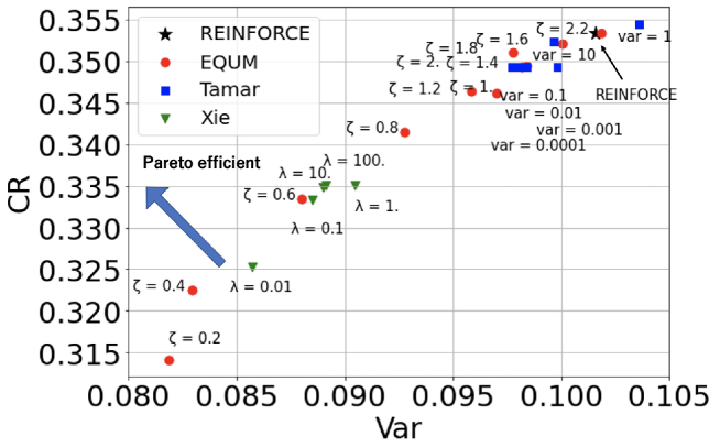
Figure 4: MV efficiency of the American-style option experiment. Higher CRs and lower Vars methods are MV Pareto efficient.

Table 3: The results of American-style option. The upper table shows the CRs and Vars over $100,000$ trials. The lower table shows The lower table shows the MSEs for $\zeta$ over $100,000$ trials.

	REINFORCE	EQUM			Tamar		Xie
	($\zeta=\infty$)	$\zeta=1.6$	$\zeta=0.8$	$\zeta=0.4$	$\mathrm{var}=1$	$\mathrm{var}=0.1$	$\lambda=100$	$\lambda=0.1$
CR	0.353	0.352	0.341	0.322	0.352	0.349	0.335	0.333
Var	0.099	0.098	0.092	0.083	0.102	0.096	0.089	0.088

	REINFORCE	EQUM
Target Value	($\zeta=\infty$)	$\zeta=2.2$	$\zeta=1.8$	$\zeta=1.4$	$\zeta=1.0$	$\zeta=0.6$
MSE from $\zeta=2.2$	3.512	3.512	3.517	3.523	3.532	3.572
$\zeta=1.8$	2.194	2.195	2.197	2.203	2.209	2.239
$\zeta=1.4$	1.197	1.197	1.198	1.202	1.206	1.226
$\zeta=1.0$	0.520	0.520	0.519	0.522	0.523	0.532
$\zeta=0.6$	0.162	0.163	0.160	0.161	0.160	0.159

Appendix D Details of experiments of portfolio management with a real-world dataset

The average of real objective (minimizing variance with a penalty on return targeting) for Tamar, MVP and EQUM from July 2000 to June 2020 is shown in Table 5.

We also divide the performance period into two for robustness checks. Table 5 shows the first-half results from July 2000 to June 2010 and the second-half results from July 2010 to June 2020. In almost all cases, the EQUM portfolio achieves the highest R/R.

We plot results of Tamar, Xie, and EQUM with various parameters in Figure 5. We choose the parameter of Tamar ($\mathrm{var}$) from $\{1.5,2.5,3,4.55,5.5,6.5,7.5,8.5,9.5,10,10.5\}$, Xie ($\lambda$) from $\{10,50,100,200,300,400,500,600,700,800,900,1000\}$, and EQUM ($\zeta$) from $\{0.125,0.25,0.375,0.5,0.625,0.75,0.875,1,1.125,1.25,1.375,1.5\}$. We only annotate the points of $\mathrm{var}=1.5,4.5,6.5,9.5$, $\lambda=10,200,500,800$, and $\zeta=0.125,0.5,0.875,1.25$. Unlike Section 5.1, it is not easy to control the mean and variance owing to the difficulty of predicting the real-world financial markets. However, the EQUM tends to return more efficient results than the other methods.

Table 4: The average of real objective (minimizing variance with a penalty on return targeting) for Tamar, MVP and EQUM for FF25 dataset (upper panel) , FF48 (middle panel) and FF100 (lower panel) from July 2020 to June 2020.

	Tamar			Xie			EQUM
	2.5	5	10	10	100	1000	2/4	3/4	6/4
FF25	-5,359	-7,346	-7,444	-6,206	-6,206	-7,496	-7,620	-7,521	-8,857
FF48	-5,265	-7,252	-7,345	-6,384	-9,616	-7,369	-8,772	-8,343	-7,514
FF100	-6,600	-7,158	-6,042	-6,148	-5,327	-6,913	-9,650	-7,270	-8,269

Table 5: The performance of each portfolio during first half out-of-sample period (from July 2000 to June 2010) and second half out-of-sample period (from July 2010 to June 2020) for FF25 dataset (upper panel) , FF48 (middle panel) and FF100 (lower panel). Among the comparisons of the various portfolios, the best performance within each dataset is highlighted in bold.

FF25	EW	MV	EGO	BLD	Tamar			Xie			EQUM
					2.5	5	10	10	100	1000	0.5	0.75	1.5
First-Half Period (from July 2000 to June 2010)
CR$\uparrow$	0.58	-0.42	0.72	0.41	0.66	1.33	1.33	1.11	1.11	1.22	1.32	1.18	1.55
Var$\downarrow$	31.21	69.36	33.30	12.50	37.87	21.19	21.19	16.13	16.13	17.10	11.38	11.24	11.18
R/R$\uparrow$	0.36	-0.17	0.43	0.41	0.37	1.00	1.00	0.95	0.95	1.02	1.35	1.22	1.61
MaxDD$\downarrow$	0.54	0.75	0.57	0.37	0.33	0.31	0.31	0.22	0.22	0.21	0.18	0.14	0.13
Second-Half Period (from July 2000 to June 2010)
CR$\uparrow$	1.02	0.63	1.03	0.70	1.27	1.06	1.06	0.69	0.69	0.81	0.71	0.44	0.95
Var$\downarrow$	25.92	37.24	27.92	11.47	59.68	46.84	46.79	45.75	45.75	15.32	25.70	13.27	18.67
R/R$\uparrow$	0.69	0.36	0.67	0.72	0.57	0.53	0.54	0.35	0.35	0.72	0.49	0.42	0.76
MaxDD$\downarrow$	0.31	0.50	0.31	0.22	0.64	0.58	0.58	0.57	0.57	0.30	0.36	0.30	0.31
FF48	EW	MV	EGO	BLD	Tamar			Xie			EQUM
					2.5	5	10	10	100	1000	0.5	0.75	1.5
First-Half Period (from July 2000 to June 2010)
CR$\uparrow$	0.60	0.41	0.75	0.34	1.00	0.54	0.65	1.75	1.55	1.63	1.36	1.06	0.99
Var$\downarrow$	25.85	57.50	39.33	10.97	5.99	6.79	3.64	32.45	24.67	27.32	6.69	6.50	38.49
R/R$\uparrow$	0.41	0.19	0.41	0.36	1.41	0.72	1.19	1.06	1.08	1.08	1.82	1.45	0.55
MaxDD$\downarrow$	0.53	0.58	0.53	0.38	0.05	0.15	0.04	0.25	0.24	0.21	0.05	0.15	0.45
Second-Half Period (from July 2000 to June 2010)
CR$\uparrow$	1.02	-0.12	1.33	0.69	0.01	1.03	0.60	1.13	1.24	0.13	0.61	0.99	0.90
Var$\downarrow$	19.88	96.14	24.24	8.27	22.57	30.41	32.51	63.16	55.02	39.90	16.03	32.94	26.91
R/R$\uparrow$	0.79	-0.04	0.93	0.84	0.01	0.64	0.37	0.49	0.58	0.07	0.53	0.60	0.60
MaxDD$\downarrow$	0.26	0.84	0.28	0.17	0.58	0.54	0.45	0.56	0.52	0.65	0.29	0.45	0.32
FF100	EW	MV	EGO	BLD	Tamar			MVP			EQUM
					2.5	5	10	10	100	1000	0.5	0.75	1.5
First-Half Period (from July 2000 to June 2010)
CR$\uparrow$	0.61	-0.37	0.73	0.41	1.19	1.22	1.39	1.82	0.47	1.42	1.67	1.19	1.80
Var$\downarrow$	32.02	79.35	35.11	12.43	24.05	10.48	28.38	35.08	83.87	40.80	14.33	13.42	14.15
R/R$\uparrow$	0.37	-0.15	0.43	0.40	0.84	1.31	0.90	1.07	0.18	0.77	1.52	1.12	1.65
MaxDD$\downarrow$	0.55	0.72	0.58	0.36	0.39	0.18	0.27	0.46	0.46	0.31	0.16	0.15	0.11
Second-Half Period (from July 2000 to June 2010)
CR$\uparrow$	1.01	0.66	1.00	0.66	1.43	0.76	0.88	0.63	1.44	1.24	1.06	0.70	0.39
Var$\downarrow$	26.61	35.92	29.64	11.12	41.27	23.76	38.73	51.56	79.62	46.48	25.58	17.46	14.48
R/R$\uparrow$	0.68	0.38	0.63	0.68	0.77	0.54	0.49	0.30	0.56	0.63	0.73	0.58	0.36
MaxDD$\downarrow$	0.32	0.35	0.31	0.22	0.38	0.49	0.38	0.50	0.65	0.46	0.39	0.31	0.24

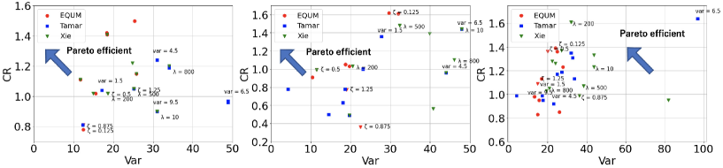
Figure 5: MV efficiency of the portfolio management experiment. Higher CRs and lower Vars methods are MV Pareto efficient. Left graph: FF25. Center graph: FF48. Right graph: FF100.

Appendix E Actor-critic with EQUM

For another combination with the EQUM framework, we apply an actor-critic (AC) based algorithms, which is also refereed to as the advantage actor-critic (A2C) algorithm (Williams & Peng, 1991; Mnih et al., 2016). We follow the formulation of Prashanth & Ghavamzadeh (2013, 2016). Extending the AC algorithm, for an episode $k$ with the length $n$, we train the policy by a gradient defined as

$$\nabla_{\theta}\log\pi_{\theta}(S^{k}_{t},A^{k}_{t})\Bigg{\{}\left(\alpha\widetilde{R}^{k}_{t:t+n-1}-\frac{1}{2}\beta\widetilde{R}^{k,2}_{t:t+n-1}\right)-\left(\alpha M^{(1)}_{\hat{\omega}^{(1)}_{k}}(S^{k}_{t})-\frac{1}{2}\beta M^{(2)}_{\hat{\omega}^{(2)}_{k}}(S^{k}_{t})\right)\Bigg{\}},$$

where

$$\widetilde{R}^{k}_{t:t+n-1}=\widehat{R}^{k}_{t:t+n-1}+\gamma^{n}M^{(1)}_{\hat{\omega}^{(1)}_{k}}(S^{k}_{t+n}),$$

$$\widetilde{R}^{k,2}_{t:t+n-1}=\left(\widehat{R}^{k}_{t:t+n-1}\right)^{2}+2\gamma^{n}\widehat{R}^{k}_{t:t+n-1}M^{(1)}_{\hat{\omega}^{(1)}_{k}}(S^{k}_{t+n})+\gamma^{2n}M^{(2)}_{\hat{\omega}^{(2)}_{k}}(S^{k}_{t+n}),$$

and $M^{(1)}_{\hat{\omega}^{(1)}_{k}}(S^{k}_{t})$ and $M^{(2)}_{\hat{\omega}^{(2)}_{k}}(S^{k}_{t})$ are value functions approximating $\mathbb{E}[R_{t+1:\infty}]$ and $\mathbb{E}[R^{2}_{t+1:\infty}]$ with parameters $\hat{\omega}^{(1)}_{k}$ and $\hat{\omega}^{(2)}_{k}$, respectively. For more details, see Prashanth & Ghavamzadeh (2013, 2016).

References

- Baron (1977) Baron, D. P. On the utility theoretic foundations of mean-variance analysis. The Journal of Finance, 32, 1977.
- Baxter & Bartlett (2001) Baxter, J. and Bartlett, P. L. Infinite-horizon policy-gradient estimation. Journal of Artificial Intelligence Research, 15:319–350, 2001.
- Bertsekas & Tsitsiklis (1995) Bertsekas, D. P. and Tsitsiklis, J. N. Neuro-dynamic programming: An overview. In Proceedings of 1995 34th IEEE Conference on Decision and Control, volume 1, pp. 560–564. IEEE, 1995.
- Bisi et al. (2020) Bisi, L., Sabbioni, L., Vittori, E., Papini, M., and Restelli, M. Risk-averse trust region optimization for reward-volatility reduction. In Proceedings of the Twenty-Ninth International Joint Conference on Artificial Intelligence, 2020.
- Bodnar et al. (2015a) Bodnar, T., Parolya, N., and Schmid, W. On the exact solution of the multi-period portfolio choice problem for an exponential utility under return predictability. European Journal of Operational Research, 246(2):528–542, 2015a.
- Bodnar et al. (2015b) Bodnar, T., Parolya, N., and Schmid, W. A closed-form solution of the multi-period portfolio choice problem for a quadratic utility function. Annals of Operations Research, 229(1):121–158, 2015b.
- Bodnar et al. (2018) Bodnar, T., Okhrin, Y., Vitlinskyy, V., and Zabolotskyy, T. Determination and estimation of risk aversion coefficients. Computational Management Xcience, 15(2):297–317, 2018.
- Borch (1969) Borch, K. A Note on Uncertainty and Indifference Curves. The Review of Economic Studies, 1969.
- Boyd & Vandenberghe (2004) Boyd, S. and Vandenberghe, L. Convex Optimization. Cambridge University Press, 2004.
- Brandt (2010) Brandt, M. W. Portfolio choice problems. In Handbook of Financial Econometrics: Tools and Techniques, pp. 269–336. Elsevier, 2010.
- Brockman et al. (2016) Brockman, G., Cheung, V., Pettersson, L., Schneider, J., Schulman, J., Tang, J., and Zaremba, W. Openai gym, 2016.
- Bulmuş & Özekici (2014) Bulmuş, T. and Özekici, S. Portfolio selection with hyperexponential utility functions. OR spectrum, 36(1):73–93, 2014.
- Chow & Ghavamzadeh (2014) Chow, Y. and Ghavamzadeh, M. Algorithms for cvar optimization in mdps. Advances in Neural Information Processing Systems, 27:3509–3517, 2014.
- Chow et al. (2017) Chow, Y., Ghavamzadeh, M., Janson, L., and Pavone, M. Risk-constrained reinforcement learning with percentile risk criteria. The Journal of Machine Learning Research, 18(1):6070–6120, 2017.
- DeMiguel et al. (2009) DeMiguel, V., Garlappi, L., and Uppal, R. Optimal versus naive diversification: How inefficient is the 1/n portfolio strategy? The Review of Financial Studies, 22(5):1915–1953, 2009.
- Fama & French (1992) Fama, E. F. and French, K. R. The cross-section of expected stock returns. The Journal of Finance, 1992.
- Fishburn & Burr Porter (1976) Fishburn, P. C. and Burr Porter, R. Optimal portfolios with one safe and one risky asset: Effects of changes in rate of return and risk. Management science, 22(10):1064–1073, 1976.
- Garcıa & Fernández (2015) Garcıa, J. and Fernández, F. A comprehensive survey on safe reinforcement learning. Journal of Machine Learning Research, 16(1):1437–1480, 2015.
- Geibel & Wysotzki (2005) Geibel, P. and Wysotzki, F. Risk-sensitive reinforcement learning applied to control under constraints. Journal of Artificial Intelligence Research, 24:81–108, 2005.
- Kallberg et al. (1983) Kallberg, J., Ziemba, W., et al. Comparison of alternative utility functions in portfolio selection problems. Management Science, 29(11):1257–1276, 1983.
- Kroll et al. (1984) Kroll, Y., Levy, H., and Markowitz, H. M. Mean-variance versus direct utility maximization. The Journal of Finance, 39(1):47–61, 1984.
- Lintner (1965) Lintner, J. The valuation of risk assets and the selection of risky investments in stock portfolios and capital budgets. Review of Economics and Statistics, 47(1):13–37, 1965.
- Luenberger et al. (1997) Luenberger, D. G. et al. Investment science. OUP Catalogue, 1997.
- Magdon-Ismail & Atiya (2004) Magdon-Ismail, M. and Atiya, A. F. Maximum drawdown. Risk Magazine, 2004.
- Markowitz (1952) Markowitz, H. Portfolio selection. The Journal of Finance, 1952.
- Markowitz (1959) Markowitz, H. Portfolio selection: efficient diversification of investments. Yale university press, 1959.
- Markowitz & Todd (2000) Markowitz, H. M. and Todd, G. P. Mean-Variance Analysis in Portfolio Choice and Capital Markets, volume 66. John Wiley & Sons, 2000.
- Mas-Colell et al. (1995) Mas-Colell, A., Whinston, M. D., Green, J. R., et al. Microeconomic Theory, volume 1. Oxford university press New York, 1995.
- Merton (1969) Merton, R. C. Lifetime portfolio selection under uncertainty: The continuous-time case. The Review of Economics and Statistics, pp. 247–257, 1969.
- Mnih et al. (2016) Mnih, V., Badia, A. P., Mirza, M., Graves, A., Lillicrap, T., Harley, T., Silver, D., and Kavukcuoglu, K. Asynchronous methods for deep reinforcement learning. In International Conference on Machine Learning, pp. 1928–1937, 2016.
- Morgenstern & Von Neumann (1953) Morgenstern, O. and Von Neumann, J. Theory of games and economic behavior. Princeton University Press, 1953.
- Mossin (1966) Mossin, J. Equilibrium in a capital asset market. Econometrica: Journal of the econometric society, pp. 768–783, 1966.
- Prashanth & Ghavamzadeh (2013) Prashanth, L. and Ghavamzadeh, M. Actor-critic algorithms for risk-sensitive mdps. In Proceedings of the 26th International Conference on Neural Information Processing Systems-Volume 1, pp. 252–260, 2013.
- Prashanth & Ghavamzadeh (2016) Prashanth, L. and Ghavamzadeh, M. Variance-constrained actor-critic algorithms for discounted and average reward mdps. Machine Learning, 105(3):367–417, 2016.
- Puterman (1994) Puterman, M. L. Markov Decision Processes: Discrete Stochastic Dynamic Programming. John Wiley & Sons, 1994.
- Schulman et al. (2015) Schulman, J., Levine, S., Abbeel, P., Jordan, M., and Moritz, P. Trust region policy optimization. In International Conference on Machine Learning, pp. 1889–1897, 2015.
- Sharpe (1964) Sharpe, W. F. Capital asset prices: A theory of market equilibrium under conditions of risk. The Journal of Finance, 19(3):425–442, 1964.
- Sharpe (1966) Sharpe, W. F. Mutual fund performance. The Journal of Business, 1966.
- Shen & Wang (2016) Shen, W. and Wang, J. Portfolio blending via thompson sampling. In Proceedings of the Twenty-Fifth International Joint Conference on Artificial Intelligence, pp. 1983–1989, 2016.
- Shen et al. (2019) Shen, W., Wang, B., Pu, J., and Wang, J. The kelly growth optimal portfolio with ensemble learning. In Proceedings of the AAAI Conference on Artificial Intelligence, volume 33, pp. 1134–1141, 2019.
- Sutton & Barto (1998) Sutton, R. S. and Barto, A. G. Reinforcement Learning: An Introduction. The MIT Press, 1998.
- Sutton et al. (2000) Sutton, R. S., McAllester, D. A., Singh, S. P., and Mansour, Y. Policy gradient methods for reinforcement learning with function approximation. In Advances in Neural Information Processing Systems, pp. 1057–1063, 2000.
- Tamar et al. (2012) Tamar, A., Di Castro, D., and Mannor, S. Policy gradients with variance related risk criteria. In Proceedings of the 29th International Coference on International Conference on Machine Learning, pp. 1651–1658, 2012.
- Tamar et al. (2014) Tamar, A., Mannor, S., and Xu, H. Scaling up robust mdps using function approximation. In International Conference on Machine Learning, pp. 181–189, 2014.
- Tobin (1958) Tobin, J. Liquidity preference as behavior towards risk. The Review of Economic Studies, 25(2):65–86, 1958.
- Williams (1988) Williams, R. Toward a Theory of Reinforcement-learning Connectionist Systems. Northeastern University, 1988.
- Williams (1992) Williams, R. J. Simple statistical gradient-following algorithms for connectionist reinforcement learning. Machine learning, 8(3-4):229–256, 1992.
- Williams & Peng (1991) Williams, R. J. and Peng, J. Function optimization using connectionist reinforcement learning algorithms. Connection Science, 3(3):241–268, 1991.
- Xie et al. (2018) Xie, T., Liu, B., Xu, Y., Ghavamzadeh, M., Chow, Y., Lyu, D., and Yoon, D. A block coordinate ascent algorithm for mean-variance optimization. Advances in Neural Information Processing Systems, 31:1065–1075, 2018.
- Zhang et al. (2021) Zhang, S., Liu, B., and Whiteson, S. Mean-variance policy iteration for risk-averse reinforcement learning. In Thirty-Fifth AAAI Conference on Artificial Intelligence, 2021.
- Ziemba et al. (1974) Ziemba, W., Parkan, C., and Brooks-Hill, R. Calculation of investment portfolios with risk free borrowing and lending. Management Science, 21(2), 1974.