Physics-based Reconstruction Methods for Magnetic Resonance Imaging

Abstract

Conventional Magnetic Resonance Imaging (MRI) is hampered by long scan times and only qualitative image contrasts that prohibit a direct comparison between different systems. To address these limitations, model-based reconstructions explicitly model the physical laws that govern the MRI signal generation. By formulating image reconstruction as an inverse problem, quantitative maps of the underlying physical parameters can then be extracted directly from efficiently acquired k-space signals without intermediate image reconstruction – addressing both shortcomings of conventional MRI at the same time. This review will discuss basic concepts of model-based reconstructions and report about our experience in developing several model-based methods over the last decade using selected examples that are provided complete with data and code.

1 Introduction

First physics-based reconstruction methods for parametric mapping appeared in the literature more than a decade ago [1, 2, 3] and constitute now a major research area in the field of Magnetic Resonance Imaging (MRI) [4, 5, 6, 7, 8, 9, 10, 11, 12, 13]. Model-based reconstruction is based on modelling the physics of the MRI signal and has been used, for example, to estimate T1 [14, 6, 9, 15, 13, 16], T2 relaxation [3, 5, 10, 17], for T2^⋆ estimation and water-fat separation [18, 19, 20, 21, 22], as well as for quantification of flow [11] and diffusion [23, 24]. Quantitative maps of the underlying physical parameters can then be extracted directly from the measurement data without intermediate image reconstruction. This direct reconstruction has two major advantages: First, the full signal is described by a model based on few parameter maps only and intermediate image reconstruction is waived. This renders model-based techniques much more efficient in exploiting the available information than conventional two-step methods. Second, as a specific signal behaviour is no longer required for image reconstruction, MRI sequences can now be designed that have an optimal sensitivity to the parameters of interest. Once the underlying physical parameters are estimated, arbitrary contrast-weighted images can be generated synthetically by evaluating the signal model for a specific sequence and acquisition parameters.

In this work, we discuss our experience using model-based reconstruction methods with different radial MRI sequences showing a variety of examples ranging from T1 and T1 mapping and banding-free bSSFP imaging in the brain over flow quantification in the aorta to water-fat separation and $T_{2}^{\star}$ mapping in the liver. All provided examples come with data and code and can be reconstructed using the BART toolbox [25].

2 MRI Signal

In typical MRI experiments, the proton spins are polarized by bringing them into a strong external field. The spins then start to precess with a characteristic Larmor frequency and can be manipulated using additional on-resonant radio-frequency pulses and further gradient fields. The dynamical behaviour of the magnetization is described by the Bloch-Torrey equations that describe the physics of magnetic resonance including effects from relaxation, flow and diffusion. As a fully computer-controlled imaging method, MRI is extremely flexible and the underlying physics enables access to a variety of tissue and imaging system specific parameters such as relaxation constants, flow velocities, diffusion, temperature, magnetic fields, etc.

The measured MRI signal corresponds to the complex-valued transversal magnetization $M$ which is obtained by quadrature demodulation from the voltage induced in the receive coils. In a multi-coil experiment this signal is proportional to the transversal magnetization weighted by the sensitivity of each receive coil:

$$y_{j}(t)=\int c_{j}(\vec{r})\,M(x,B,t,\vec{r})\,d\vec{r}$$ (1)

Here, $c_{j}$ is the complex-valued sensitivity of the $j$th coil and $M$ the complex-valued transversal magnetization at time $t$ and position $\vec{r}$. The magnetization depends on some physical parameters $x$ and the externally controlled magnetic fields $B(t,\vec{r})$, i.e. gradient fields and radio-frequency pulses, and can be obtained by solving the Bloch-Torrey equations (or, if motion of spins can be neglected, by solving the Bloch equations at each point).

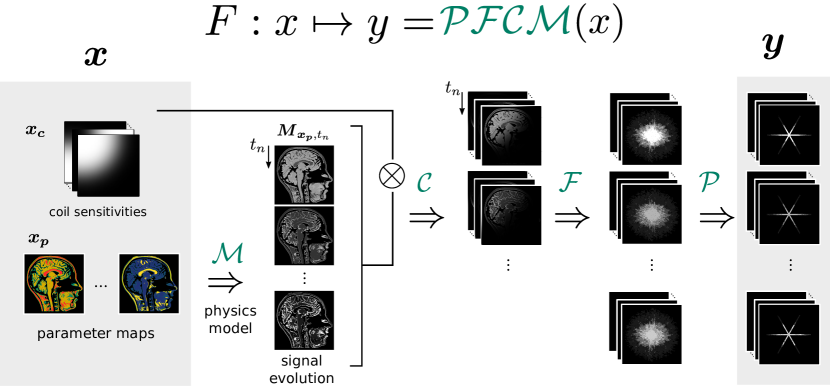
Figure 1: The forward operator $F$ can be formally factorized into operator $\mathcal{M}$ that describes the spin physics, the multiplication with the coil sensitivities $\mathcal{C}$, the (non-uniform) Fourier transform $\mathcal{F}$, and a sampling operator $\mathcal{P}$.

parameter	sequence type	signal
relaxation rate $R_{1}$	inversion recovery	$a-(1+a)\cdot e^{-t_{n}\nicefrac{{R_{1}}}{{a}}}$
relaxation rate $R_{2}$	spin-echo	$e^{-R_{2}t_{n}}$
relaxation rate $R_{2}^{\star}$	gradient-echo	$e^{-{R_{2}^{*}}t_{n}}$
field $B_{0}$	gradient-echo	$e^{i2\pi\cdot f_{B_{0}}t_{n}}$
chemical shift	gradient-echo	$\sum_{p}e^{i2\pi f_{p}t_{n}}$
flow velocity $\vec{v}$	bipolar gradient	$e^{i\vec{v}\cdot\vec{V}_{n}}$
diffusion tensor $D$	bipolar gradient	$e^{-\vec{b}_{n}^{T}Db_{n}}$

Table 1: Basic analytical signal models for physical parameter dependencies in common MRI sequences.

While Equation (1) can be exploited directly for model-based reconstruction [26], many other model-based methods use some simplifying approximations to reduce the computational complexity. Often, segmentation in time is used by assuming that the magnetization is constant around certain time points, e.g. around echo times $\text{TE}_{n}$ with $n\in 1,\dots,N$. $N$ is the number of echos. The effect of magnetic field gradients can then be separated out into a phase term which is defined by the k-space trajectory $\vec{k}(t)$. This separation often allows the use of simplified models for the magnetization and, more importantly, the use of fast (non-uniform) Fourier transform algorithms for the gradient-encoding term. We derive the following - still very generic - model:

$$y_{n,j}(t) =\int e^{i2\pi\vec{r}\cdot\vec{k}(t)}c_{j}(\vec{r})M(x,t_{n},\vec{r})d\vec{r}$$ (2)

Based on this model, we define a nonlinear forward operator $F:x\mapsto y$ that maps the unknown parameters $x$ to the acquired data $y$. This operator can be formally decomposed into $F=\mathcal{PFCM}$, where $\mathcal{P}$ is the sampling operator, $\mathcal{F}$ is the Fourier transform, $\mathcal{C}$ the multiplication with the coil sensitivities, and $\mathcal{M}$ the signal model (see Fig. 1).

The defining feature of physics-modelling reconstruction is the addition of a signal model $\mathcal{M}$ into the forward operator $F$. The specific signal model depends on the applied sequence protocol and specifies which tissue and/or hardware characteristics can be estimated. Often, an analytical model can be derived from the Bloch equations using hard-pulse approximations. For many typical MRI sequences important parameter dependencies are exponentials. Table 1 lists some of these analytical signals models. If the applied sequence protocol does not lend itself to an analytical signal expression, the Bloch equations need to be integrated as signal model directly. This integration becomes challenging for iterative reconstructions, because of the estimation of the signals derivatives. Current techniques exploit finite difference methods [10, 26] or sensitivity analysis of the Bloch equations [27].

Sequence Flip Angle TR/TE/$\Delta$TE Bandwidth Matrix Spokes TA FOV Slice $\mathrm{\SIUnitSymbolDegree}$ ms Hz/px s mm mm IR-FLASH 6 4.10 / 2.58 630 256 $\times$ 256 1020 4 192 5 ME-SE 90/180 2500 / 9.9 / 9.9 390 256 $\times$ 256 25 $\times$ 16 80 192 3 ME-FLASH 5 10.60 / 1.37 / 1.34 960 200 $\times$ 200 33 $\times$ 7 0.35 ¹ 320 5 PC-FLASH 10 4.46 / 2.96 1250 210 $\times$ 210 2 $\times$ 7 15 320 5 fmSSFP² 15 4.5 / 2.25 840 192 $\times$ 192 4 $\times$ 101 $\times$ 40 137 192 1

• acquisition time per frame, because the presented example is based on
  dynamic acquisition

• 3D Stack-Of-Stars sequence with 40 partitions (1000 prep scans), while all
  other acquisition protocols are 2D

Detailed parameters of MR sequences capable of mapping physical parameters listed in Table 1.

The MRI data used in this work was acquired on a Siemens Skyra 3T scanner (Siemens Healthcare GmbH, Erlangen, Germany) from four volunteers (21-35 years, two females) without known illness after obtaining written informed consent and with approval of the local ethics committee. Acquisition parameters can be found in Table 1.

3 Nonlinear Reconstruction

Using a nonlinear forward operator $F:x\mapsto y$ that maps the unknown parameters $x$ to the acquired data $y$, we can formulate the image reconstruction as a nonlinear optimization problem:

$$\hat{x}=\operatorname*{\arg\!\min}_{x}\|F(x)-y\|_{2}^{2}+\sum_{i}\lambda_{i}R_{i}(x)$$ (3)

Data fidelity is ensured by $\|F(x)-y\|_{2}^{2}$ and regularization terms $R_{i}$ can be added to introduce prior knowledge with $\lambda_{i}$ the corresponding regularization parameters. This framework is very general, combining parallel imaging, compressed sensing, and model-based reconstruction in a unified reconstruction. Often the coil sensitivities are estimated before, but they could also be included as unknowns in $x$. Paired with suitable sampling schemes, this yields fully calibrationless methods that do not require additional calibration scans [13, 28, 29, 11, 30, 31]. Moreover, model-based reconstructions allow a direct application of sparsity-promoting regularizations to the physical parameters for performance improvement [3, 7, 24, 13].

However, the high non-convexity of model-based reconstruction makes this method sensible to the initial guess and relative scaling of the derivatives of each parameter map. These issues can often be addressed with a reasonable initial guess and a proper preconditioning. Algorithms to solve the nonlinear inverse problems include gradient descent, the variable projection methods [32, 7], the method of nonlinear conjugate gradient [33] and Newton-type methods [34]. Particularly for the examples presented in this paper, we solve Equation (3) via an iteratively regularized Gauss-Newton method (IRGNM) [34] where the nonlinear problem in Equation (3) is linearized in each Gauss-Newton step, i.e.

$$\hat{x}_{n+1}=\operatorname*{\arg\!\min}_{x}\|DF(x_{n})(x-x_{n})+F(x_{n})-y\|_{2}^{2}+\sum_{i}\lambda_{i}R_{i}(x)$$ (4)

with $DF(x_{n})$ the Jacobian matrix of $F$ at the point $x_{n}$. The regularized linear subproblem can be further solved by conjugate gradients, FISTA [35] or ADMM[36].

3.1 T1 and T2 Mapping

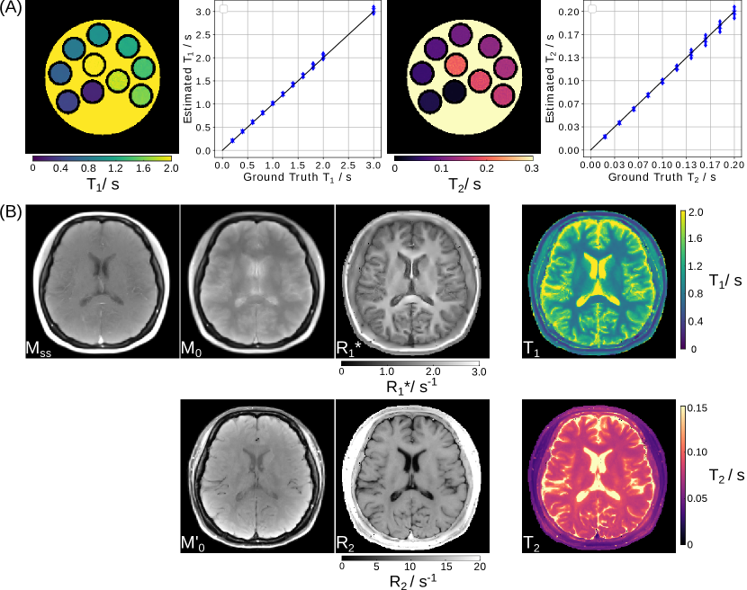
Figure 2: (A). (Leftmost) Model-based reconstructed T1 map and (left middle) the ROI-analysed quantitative T1 values for the numerical phantom using the single-shot IR radial FLASH sequence. (Right middle and rightmost) Similar results for T2 mapping using the multi-echo spin-echo sequence. (B). (Top) The reconstructed parameter maps $(M_{ss},M_{0},R_{1}^{*})^{T}$ for the T1 model and (bottom) $(M_{0},R_{2})^{T}$ for the T2 model with the corresponding T1 / T2 maps in the rightmost column.

T1 mapping can be accomplished using a inversion-recovery (IR) FLASH sequence: Following a inversion pulse, data is continuously acquired using the FLASH readout. The magnetization signal $M(t)$ for IR-FLASH reads [37, 38]

$$M_{t_{k}}(\vec{r})=M_{ss}(\vec{r})-\big{(}M_{ss}(\vec{r})+M_{0}(\vec{r})\big{)}\cdot e^{-t_{k}\cdot R_{1}^{*}(\vec{r})}$$ (5)

with $M_{ss}$ the steady-state magnetization, $M_{0}$ the equilibrium magnetization, and $R_{1}^{*}$ the effective relaxation rate, i.e. $R_{1}^{*}=1/T_{1}^{*}$. $t_{k}$ is the inversion time defined as the center of each acquisition window. The acquisition window is determined by the product of repetition time and the number of readouts formulating one k-space (binning) after inversion. Although model-based reconstructions don’t require any binning, this process is helpful for reducing the computation demand while still keeping the $T_{1}$ accuracy [13]. After estimation of $M_{ss},M_{0}$ and $R_{1}^{*}$, $T_{1}$ then can be calculated afterwards by: $T_{1}=M_{0}/(M_{ss}\cdot R_{1}^{*})$. Data for T1 mapping is acquired using a single-shot IR radial FLASH (4 seconds) sequence with a tiny golden angle ($\approx 23.36^{\circ}$) between successive spokes.

The multi-echo spin echo (ME-SE) sequence can be employed for T2 mapping. The magnetization signal $M(t)$ for a multi-echo spin echo sequence at echo time $t_{k}$ follows an exponential decay $M_{t_{k}}(\vec{r})=M^{\prime}_{0}\cdot e^{-t_{k}\cdot R_{2}(\vec{r})}$ with $M^{\prime}_{0}$ the spin density map, $R_{2}=1/T_{2}$ the transverse relaxation rate. This simple exponential model does not take stimulated echoes into account, but a more complicated analytical model exists for this case [39, 40]. Data for T2 mapping is obtained with 25 excitations and 16 echoes per excitation using a radial golden-ratio ($\approx 111.25^{\circ}$) sampling strategy.

Quantitative parameter maps for both acquisitions are estimated using the nonlinear model-based reconstruction. In other words, the estimation of parameter maps $(M_{ss},M_{0},R_{1}^{*})^{T}$ or parameter maps $(M^{\prime}_{0},R_{2})^{T}$, respectively, and coil sensitivity maps $(c_{1},\ldots,c_{N})^{T}$ is formulated as a nonlinear inverse problem with a joint $\ell_{1}$-Wavelet regularization applied to the parameter maps and the Sobolev norm [41] to the coil sensitivity maps. This nonlinear inverse problem is then solved by the IRGNM-FISTA algorithm [13]. After estimation of the parameters $T_{1}$ and $T_{2}$ maps can be calculated. Note that the $M_{0}$ and $M^{\prime}_{0}$ absorb physical effects which are not explicitely modelled and identical over all inversion or echo times.

To evaluate the quantitative accuracy of the model-based methods, numerical phantoms with different T1 relaxation times (ranging from 200 ms to 2000 ms with a step size of 200 ms for each tube, and 3000 ms for the background), T2 relaxation times (ranging from 20 ms to 200 ms with a step size of 20 ms for each tube, and 1000 ms for the background) were simulated, respectively. To avoid an inverse crime [42], the $k$-space data was derived from the analytical Fourier representation of an ellipse assuming an array of eight circular receiver coils surrounding the phantom without overlap. Complex white Gaussian noise with a moderate standard deviation was added to the simulated $k$-space data.

Fig. 2 (A) presents the estimated T1, T2 maps and the corresponding ROI-analyzed quantitative values for the numerical phantom using model-based reconstructions. Good quantitative accuracy is confirmed for both model-based T1 and T2 mapping methods. Fig. 2 (B) demonstrates model-based reconstructed three and two physical parameter maps, the corresponding T1 and T2 maps for the retrospective T1 and T2 models on human brain studies. Further, synthetic images were computed for all inversion/echo times and the image series was then converted into movies showing the contrast changes in Supplementary Videos 1 and 2. For the data presented here, model-based T1 and T2 reconstruction took around 6 and 3 minutes on a GPU (Tesla V100 SXM2, NVIDIA, Santa Clara, CA), respectively.

3.2 Water/Fat Separation and $R_{2}^{*}$ Mapping

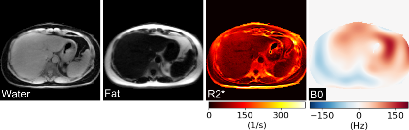
Figure 3: Real-time liver images acquired during free-breathing using a radial multi-echo (ME) FLASH sequence. Model-based reconstruction directly and jointly estimates separated water and fat images, as well as $R_{2}^{\star}$ and $B_{0}$ field maps.

Quantitative $T_{2}^{*}$ mapping can be achieved via multi-echo gradient-echo sampling. With prolonged echo-train readout, the acquired multi-echo signal is

$$M_{n}=\rho\cdot e^{-{R_{2}^{*}}\cdot\text{TE}_{n}}\cdot e^{i2\pi\cdot f_{B_{0}}\cdot\text{TE}_{n}}$$ (6)

where $R_{2}^{*}$ is the inverse of $T_{2}^{*}$ and $f_{B_{0}}$ is the $B_{0}$ field inhomogeneity. $\text{TE}_{n}$ denotes the $n$th echo time. On the other hand, when the imaging voxel contains distinct protons resonating at different frequencies, the magnetization $\rho$ can be split into multiple compartments. For instance, chemical shift between water and fat induces phase modulation, therefore,

$$M_{n}=(\text{W}+\text{F}\cdot\sum_{p}e^{i2\pi f_{p}\cdot\text{TE}_{n}})\cdot e^{-{R_{2}^{*}}\cdot\text{TE}_{n}}\cdot e^{i2\pi\cdot f_{B_{0}}\cdot\text{TE}_{n}}$$ (7)

where W and F are the water and fat magnetization, respectively. $f_{p}$ is the $p$th fat-spectrum peak frequency. In practice, usually the 6-peak fat spectrum [43] is used. In the model-based reconstruction formulation, the unknowns contain W, F, $R_{2}^{*}$, and $f_{B_{0}}$, as well as a set of coil sensitivity maps from the parallel imaging model.

Here, a multi-echo (ME) radial FLASH sequence [31] was used to acquire liver data during free breathing. The model-based reconstruction was initialized by the estimate from model-based 3-point water/fat separation [31], while $R_{2}^{*}$ and coil sensitivity maps were initialized with 0. Afterwards, joint estimation of all unknowns in Equation (7) including coil sensitivity maps was achieved via IRGNM with ADMM. The Sobolev-norm weight [41] was applied to the $B_{0}$ field inhomogeneity and coil sensitivity maps. Joint $\ell 1$-Wavelet regularization was applied to other parameter maps. As shown in Figure 3 and Supplementary Video 3, high-quality respiratory-resolved water/fat separation as well as $R_{2}^{*}$ and $f_{B_{0}}$ maps can be achieved even with undersampled multi-echo radial acquisition (33 spokes per echo and 7 echoes in total).

3.3 Phase-Contrast Velocity Mapping

In phase-contrast flow MRI, velocity-encoding gradients are used to encode flow-induced phases. Due to the complexity of MR signal, a reference measurement without flow-encoding gradients is required such that the phase difference between these two measurements excludes the background phase. Therefore, the phase-contrast flow MRI signal can be modeled as

$$M_{k}=\rho\cdot e^{i\vec{v}\cdot\vec{V}_{k}}\;.$$ (8)

$\vec{v}$ is the velocity and $V_{k}$ is the velocity-encoding for the $k$th measurement. For through-plane velocity mapping, $V_{0}=0$ for the reference and $V_{1}=\pi/\text{VENC}$ the velocity-encoded measurement, respectively. VENC is the maximum measurable velocity. $\rho$ is the shared anatomical image between the two measurements.

As an example, flow MRI sequence with radial sampling and through-plane velocity-encoding gradient was used to measure aortic blood flow velocities. As shown in Fig. 4, with direct regularization on the phase-difference map, the proposed model-based reconstruction [11, 30] is able to largely remove background random phase noise. Supplementary Video 4 displays the dynamic velocity maps of the whole 15-second scan.

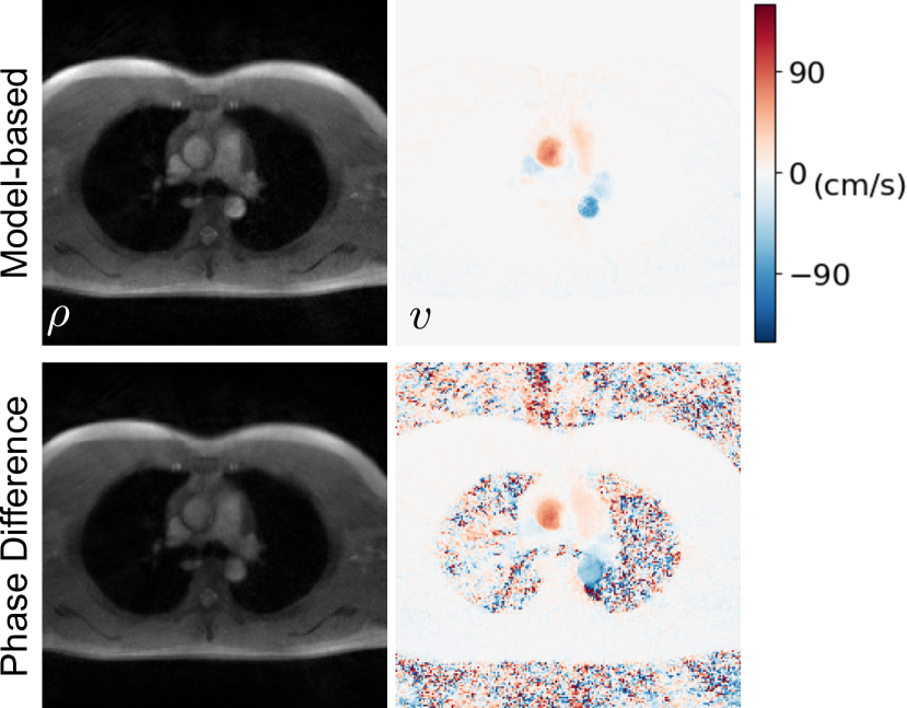
Figure 4: Comparison between (top) the model-based reconstruction and (bottom) the conventional phase-difference reconstruction. A section crossing the ascending and descending aorta was selected as the imaging slice. Displayed images are (left) anatomical magnitude image and (right) phase-contrast velocity map at systole. With direct phase-difference regularization, the model-based reconstruction largely reduces random background phase noise in the velocity map.

4 Linear Subspace Reconstruction

In contrast to nonlinear models, in linear subspace methods the signal curves $t\mapsto M(x,t,\vec{r})$ are approximated using a linear combination of basis functions [44, 45, 46, 47, 48, 49, 50, 51, 52]. , i.e.

$$M(x,t,\vec{r})\approx\sum_{s}a_{s}(\vec{r})B_{s}(t)~{}.$$ (9)

The linear basis functions $B_{s}(t)$ can be generated by simulating a set of representative signal curves for a range of parameters and performing a singular value decomposition to obtain a good representation.

With known coil sensitivities, this leads to a linear inverse problem for the subspace coefficients:

$$\hat{a}=\operatorname*{\arg\!\min}_{a}\|\mathcal{P}\mathcal{F}\mathcal{C}Ba-y\|_{2}^{2}+\sum_{i}\lambda_{i}R_{i}(a)$$ (10)

After reconstruction of the subspace coefficients $a_{s}$, the parameters $x$ need to be estimated in a separate step. This can be achieved by predicting complete magnetization maps for all time points and fitting a nonlinear signal model. This can be done point-wise, so is much easier than doing a full nonlinear reconstruction. Still, for multi-parametric mapping efficient techniques to map between coefficients and parameters are required [51].

Linear subspace methods have several advantages. Linear subspace models lead to linear inverse problems which do not have local minima. Due to their linearity, they also inherently avoid model violations stemming from partial volume effects. Because the matrix multiplication with the basis commutes with other operations that are identical at each time point, is is possible to combine the basis with the sampling operator. The reconstruction then admits a computationally advantageous formulation that allows computation to performed entirely in the subspace [46, 47].

4.1 T1 Mapping

Alternatively, T1 maps were also reconstructed using the subspace method. Similar to [50], the T1 dictionary was constructed using 1000 different $1/R_{1}^{*}$ values linearly range from 5–5000 ms, combining with 100 $M_{ss}$ values from $0.01\cdot M_{0}$ to $M_{0}$. This results in 100,000 exponential curves in the dictionary. A subset of such a dictionary is shown in Fig. 5 (left). The other parameters are TR = 4.10 ms, 20 spokes per frame, 51 frames in total. The simulated curves are highly correlated and can be represented by only a few principle components Fig. 5. For easier comparison, the subspace-constraint reconstruction used the coil sensitivity maps estimated using model-based T1 reconstruction. The resulting linear problem was then solved using conjugate gradient or FISTA algorithm in BART. The coefficient maps were then projected back to image series where the 3‐parameter fit is applied for each voxel according to Equation (5).

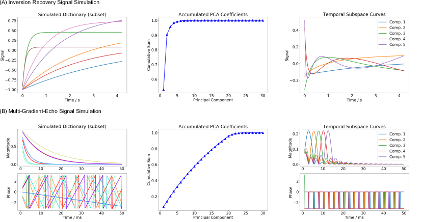
Figure 5: Demonstration of subspace-based methods for (A) single-shot inversion-recovery and (B) multi-gradient-echo signal, respectively. (Left) Simulated (top) T1 relaxation and (bottom) $T_{2}^{*}$ relaxation and off-resonance phase modulation curves. (Center) Plot of the first 30 principle components. (Right) The temporal subspace curves that can be linearly combined to form (top) T1 relaxations and (bottom) multi-gradient-echo relaxations.

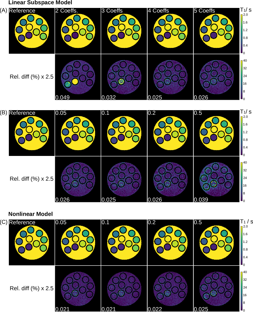
Figure 6: Comparison of linear and nonlinear model-based reconstructions on the simulated phantom. (A). Linear subspace reconstructed T1 maps using 2, 3, 4, 5 complex coefficients and their relative difference to the reference. (B). Linear subspace reconstructed T1 maps using 4 complex coefficients with changing regularization parameters. (C). Model-based reconstructed T1 maps using different regularization strengths. The numerical phantom used here is simulated using 208 frames, one spoke per frame, and TR = 20.5 ms. All reconstructions are done with L2-regularization. The regularization strength and the normalized relative errors to the reference are shown on the top-left and bottom-left of each figure, respectively.

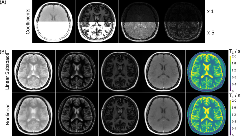
Figure 7: (A) Reconstructed 4 complex coefficient maps (only magnitude is shown) using the linear subspace method for a human brain study. (B) Synthesized images (at inversion time 40 ms, 400 ms, 800 ms, 4000 ms) using (top) the above 4 complex coefficient maps of the linear subspace method and (bottom) the 3 physical maps of the nonlinear model-based reconstruction, respectively. The corresponding T1 maps are presented in the rightmost column.

Fig. 6 (A) shows estimated phantom T1 maps using a variant number of complex coefficients of the linear subspace-based reconstruction with L2 regularization. Lower number of coefficients causes bias for quantitative T1 mapping (especially for tubes with short T1s) while higher number of coefficients brings noise in the final T1 maps. Therefore 4 coefficient maps were chosen to compromise between quantitative accuracy and precision. Fig. 6 (B) compares the effects of regularization strength. Similarly, low value of the regularization parameter brings noise while high regularization strength causes bias. A value of $0.1$ was then chosen to compromise T1 accuracy and precision. Fig. 6 (C) then shows the effects of regularization for the model-based reconstruction. A value of $0.1$ was selected as it has the least normalized error.

The low normalized relative errors on the optimized T1 maps reflect both linear subspace and nonlinear model-based methods can generate T1 maps with good accuracy while nonlinear model-based reconstruction has a slightly better performance (i.e., less normalized relative errors).

With the above settings, Fig. 7 (A) depicts the four main coefficient maps estimated using the linear subspace method for a brain study. In this case, a joint $\ell_{1}$-Wavelet sparsity regularization was applied to the maps with a strength of $0.0015$ to improve the precision. For this dataset, the reconstruction together with a pixel-wise fitting took around 2 minutes on the GPU. Fig. 7 (B) presents the synthesized images along with the corresponding T1 maps using (top) the above four coefficient maps for the linear subspace and (bottom) the 3 physical parameter maps for nonlinear model-based reconstructions, where a similar joint $\ell_{1}$-Wavelet sparsity is applied with the regularization parameter $0.09$. Again, both linear subspace and nonlinear methods could generate high-quality synthesized images and T1 maps while the nonlinear methods have slightly less noise and better sharpness.

Although linear subspace reconstruction has been demonstrated to be a fast and robust quantitative parameter mapping technique, it might not be directly applicable to MR signals with phase modulation along echo trains. For instance, multi-gradient-echo signals are known to be modulated by off-resonance-induced phases. A dictionary of multi-gradient-echo magnitude and phase signals was simulated with $256\times 256$ $T_{2}^{*}$ and $f_{B_{0}}$ combinations linearly ranging from 1 to 100 $\mathrm{ms}$ and from -200 to 200 $\mathrm{Hz}$, respectively.

Fig. 5 displays the magnitude and phase evolution of 7 randomly-selected dictionary entries. The magnitude signal follows the exponential decay, while phase wrappings occur with large field inhomogeneity and long echo train readout. More importantly, the SVD analysis of the signal dictionary shows that at least 26 principal components are required to represent the complex signal behaviour.

4.2 Frequency-Modulated SSFP

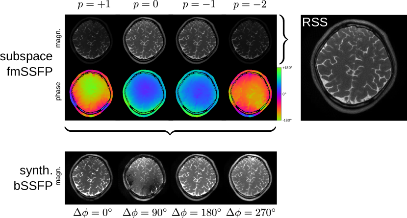
Figure 8: Reconstructed subspace coefficients maps (top) along with its root-sum-squares composite image for a individual slice within the acquired 3D volume. Synthesized bSSFP images are computed from these coefficient maps for different virtual frequency offsets (bottom).

Conventional balanced steady-state free precession (bSSFP) sequences exhibit a high signal-to-noise ratio (SNR) but suffer from possible signal voids in regions with certain off-resonance distributions. These voids or banding artifacts can be removed when multiple images are acquired with different transmitter phase cycles. Foxall and coworkers demonstrated that bSSFP sequences are tolerant to small but continuous changes in transmitter frequency [53]. In [49] we exploited this method to develop a time-efficient alternative to phase-cycled bSSFP that waives intermediate preparation phases in phase-cycled bSSFP to establish different steady-states. Image reconstruction is performed in the low-frequency Fourier subspace and yields signal intensity and contrast comparable to on-resonant bSSFP.

To this end, a frequency-modulated SSFP (fmSSFP) pulse sequence [53] was combined with 3D stack-of-stars data acquisition such that a single full sweep through the spectral response profile was obtained. Aligned partitions allowed to decouple the reconstruction problem into individual slices by a 1D inverse Fourier transform. After coil sensitivity estimation [54], image reconstruction was performed by solving a linear subspace-constrained reconstruction problem using a local low rank regularization. As a subspace basis, the four lowest order Fourier modes were chosen. Figure 8 shows the reconstructed complex-valued coefficient maps from which a composite image can be computed in a root-sum-squares manner (top). Additionally, synthesized bSSFP images are computed for four virtual frequency offsets (bottom) in which the distribution of signal voids is given by the phase distribution of the subspace coefficients. These synthesized bSSFP images correspond to conventional bSSFP images acquired with four different phase cycles.

5 Discussion

In the past decades various techniques were developed to accelerate quantitative MRI. One very general way is to exploit complementary information from spatially distinct receiver coils, called parallel imaging (PI) [55, 56, 57]. Others make use of the fact that MR images are usually sparse in a certain transform domain and combined with incoherent sampling and nonlinear image reconstruction algorithms it is called compressed sensing (CS) [58]. Exploiting this prior knowledge about a compressible image, CS can recover MR images from highly undersampled data [59, 60]. Other approaches combine PI and CS with efficient non-Cartesian sampling schemes [60].
When it comes to parameter mapping, beside of the already mentioned sparsity constraints, also low-rank constraints or joint sparsity can be exploited along the parameter dimension to accelerate the acquisition time [14, 61, 62, 63, 16].
Generally speaking, the methods above usually consist of two steps: first reconstruction of contrast-weighted images from undersampled datasets and second, the subsequent voxel-by-voxel fitting/matching. In contrast, model-based reconstructions integrate the underlying MR physics into the forward model, enabling estimation of MR physical images (parameter maps) directly from the undersampled $k$-space, bypassing the intermediate steps of image reconstruction and pixel-wise fitting/matching completely. This has the advantage of only reconstructing the desired parameter maps instead of a set of contrast-weighted images, i.e., reducing the number of unknowns tremendously. Another advantage is that parameter estimation using L2 norm in the data fidelity is optimal (assuming white Gaussian noise), while fitting reconstructed magnitude images may introduce a noise dependent bias. Special sampling strategies are required for model-based reconstruction to achieve good reconstructions. Sampling schemes used include CAIPIRINHA [64] and golden-ratio radial acquisition [65].

In contrast to non-linear model-based reconstruction methods which use a minimal number of physical parameters to describe the MR signal precisely, linear subspace methods approximate the MR signal using a certain number of principal coefficients. As discussed above, this computationally much more efficient and avoids partial volume effects. Subspace methods were also successfully used for multi-parametric imaging, for example using pseudo steady‐state free precession (pSSFP) [48] or echo planar time-resolved imaging where it is combined with non-linear iterative phase estimation [52]. Subspace methods have to balance two additional error terms coming from 1) the approximation error when the subspace size is too small and 2) noise amplification when the subspace size is large (more unknowns). To minimize these additional errors, the optimal subspace size has to be selected. While noise can be predicted based on the size of the subspace, the approximation error is more difficult to control and may require systematic studies that include comparisons to a ground truth.

Model-based reconstructions are, in general, memory demanding and time consuming as all the data has to be hold in memory simultaneously during iterations. However, modern computational devices such as GPUs have enabled faster reconstructions. For example, the computation time for model-based T1 reconstruction presented here has been reduced from around 4 hours in CPU (40‐core 2.3 GHz Intel Xeon E5‐2650 server with a RAM size of 512 GB) to 6 minutes using GPUs (Tesla V100 SXM2, NVIDIA, Santa Clara, CA). Other smart computational strategies [46, 25, 66] may also be employed to reduce the memory and computational time. The other limitation might be that model-based reconstructions are sensitive to model mismatch, e.g., bi-exponential processes, slow exchange regime. One way to overcome such limitations is to explicitly model these effects and include them into the model-based reconstruction.

Validation or the assessment of errors is an important part when developing nonlinear model-based reconstruction methods. To this end, several strategies should be applied. First, numerical simulations with analytical k-space models can assure general convergence and robustness to noise as noise levels can be freely chosen and noise-free ground truth is available. Second, in vitro or phantom studies covering a certain range of parameters of interest should be performed as effects such as intra-voxel dephasing, imperfect RF excitation, and shimming are hard to simulate and the effect of such model errors are hard to predict. Several hardware phantoms are commercially available, well charactarized and widely used [67]. Last, in vivo measurements should always be evaluated against established methods or fully-sampled data sets if possible.

Tremendous progress in the fields of machine learning / deep learning has sparked a huge interest in applying these methods to different MRI applications including image reconstruction [68, 69]. However, so far only few applications exist that target accelerated parameter mapping directly [70, 71, 72, 73]. While these are promising developments, there are also still unsolved questions regarding the stability of machine learning methods [74] and the risk of introducing image features that look real but are not present in the data (hallucinations) [75].

Magnetic Resonance Fingerprintig (MRF) [76] is an alternative technique to perform time-efficient multi-parametric mapping leveraging high undersampling factors. In its original formulation, parameter maps are reconstructed in a two-step procedere. First, time series are generated by an inverse NUFFT operation agnostic to any physical signal model. Second, parameter maps are generated by pixel-wise matching of the obtained time series with a precomputed dictionary consisting of simulated signal prototypes. The proposed decoupling into a linear reconstruction of time series and a nonlinear fitting problem solved by exhaustive search results in comparatively short reconstruction times and does not require analytical signal models. These two advantages rendered MRF a very popular approach in the recent years. This two-step procedere, however, comes at a cost. The initial model-agnostic gridding operation results in heavily aliased signal time courses. Aliasing can be removed only partially by pixel-wise matching, as no information on the sampling pattern is available in that step, and might deteriorate or bias the obtained parameter maps. Recent works have tried to overcome this inherent drawback of the two-step method by iterating between time and parameter domain [77] or by formulating the reconstruction as a nonlinear problem that integrates the physical signal model and additional image priors [7] similar to the discussed model-based approaches. Also techniques combining iterative reconstructions and grid searches on dictionaries were developed [78]. For a recent review that discusses the basic concept of MRF also in the context of other quantitative methods see [79].

6 Conclusion

By formulating image reconstruction as an inverse problem, model-based reconstruction techniques can estimate quantitative maps of the underlying physical parameters directly from the acquired k-space signals without intermediate image reconstruction. While this is computationally demanding, it enables very efficient quantitative MRI.

Funding Statement

This work was supported by the DZHK (German Centre for Cardiovascular Research), by the Deutsche Forschungsgemeinschaft (DFG, German Research Foundation) under grant TA 1473/2-1 / UE 189/4-1 and under Germany’s Excellence Strategy—EXC 2067/1‐390729940, and funded in part by NIH under grant U24EB029240.

Data Accessibility

All model-based reconstructions were performed with the BART toolbox. Scripts to reproduce the examples shown in this work are available at https://github.com/mrirecon/physics-recon.
Data is available at DOI: 10.5281/zenodo.4381986.

Competing Interests

We have no competing interests.

Author’s Contributions

All authors contributed to the design of the studies, the acquisition of the data, and the analysis. All authors helped to write the manuscript and approved the final version.

References

- [1] Graff C, Li Z, Bilgin A, Altbach MI, Gmitro AF, Clarkson EW. 2006 Iterative T2 estimation from highly undersampled radial fast spin-echo data. In Proc. Int. Soc. Mag. Reson. Med. vol. 14 p. 925.
- [2] Olafsson VT, Noll DC, Fessler JA. 2008 Fast Joint Reconstruction of Dynamic and Field Maps in Functional MRI. IEEE Trans. Med. Imag. 27, 1177–1188.
- [3] Block KT, Uecker M, Frahm J. 2009 Model-Based Iterative Reconstruction for Radial Fast Spin-Echo MRI. IEEE Trans. Med. Imaging 28, 1759–1769.
- [4] Fessler JA. 2010 Model-based image reconstruction for MRI. IEEE Signal Process. Mag. 27, 81–89.
- [5] Sumpf TJ, Uecker M, Boretius S, Frahm J. 2011 Model-based nonlinear inverse reconstruction for T2-mapping using highly undersampled spin-echo MRI. J. Magn. Reson. Imaging 34, 420–428.
- [6] Tran-Gia J, Stäb D, Wech T, Hahn D, Köstler H. 2013 Model-based acceleration of parameter mapping (MAP) for saturation prepared radially acquired data. Magn. Reson. Med. 70, 1524–1534.
- [7] Zhao B, Lam F, Liang Z. 2014 Model-Based MR Parameter Mapping With Sparsity Constraints: Parameter Estimation and Performance Bounds. IEEE Trans. Med. Imaging 33, 1832–1844.
- [8] Tran-Gia J, Wech T, Bley T, Köstler H. 2015 Model-based acceleration of Look-Locker T1 mapping. PLoS One 10, 1–15.
- [9] Roeloffs V, Wang X, Sumpf TJ, Untenberger M, Voit D, Frahm J. 2016 Model-based reconstruction for T1 mapping using single-shot inversion-recovery radial FLASH. Int. J. Imag. Syst. Tech. 26, 254–263.
- [10] Ben-Eliezer N, Sodickson DK, Shepherd T, Wiggins GC, Block KT. 2016 Accelerated and motion-robust in vivo T2 mapping from radially undersampled data using bloch-simulation-based iterative reconstruction. Magn. Reson. Med. 75, 1346–1354.
- [11] Tan Z, Roeloffs V, Voit D, Joseph AA, Untenberger M, Merboldt KD, Frahm J. 2017 Model-based reconstruction for real-time phase-contrast flow MRI: Improved spatiotemporal accuracy. Magn. Reson. Med. 77, 1082–1093.
- [12] Sbrizzi A, Bruijnen T, van der Heide O, Luijten P, van den Berg CAT. 2017 Dictionary-free MR Fingerprinting reconstruction of balanced-GRE sequences. arXiv e-prints.
- [13] Wang X, Roeloffs V, Klosowski J, Tan Z, Voit D, Uecker M, Frahm J. 2018 Model-based T1 mapping with sparsity constraints using single-shot inversion-recovery radial FLASH. Magn. Reson. Med. 79, 730–740.
- [14] Doneva M, Börnert P, Eggers H, Stehning C, Sénégas J, Mertins A. 2010 Compressed sensing reconstruction for magnetic resonance parameter mapping. Magn. Reson. Med. 64, 1114–1120.
- [15] Tran-Gia J, Bisdas S, Köstler H, Klose U. 2016 A model-based reconstruction technique for fast dynamic T1 mapping. Magn. Reson. Imaging 34, 298–307.
- [16] Maier O, Schoormans J, Schloegl M, Strijkers GJ, Lesch A, Benkert T, Block T, Coolen BF, Bredies K, Stollberger R. 2019 Rapid T1 quantification from high resolution 3D data with model-based reconstruction. Magn. Reson. Med. 81, 2072–2089.
- [17] Hilbert T, Sumpf TJ, Weiland E, Frahm J, Thiran JP, Meuli R, Kober T, Krueger G. 2018 Accelerated T2 mapping combining parallel MRI and model-based reconstruction: GRAPPATINI. J. Magn. Reson. Imaging 48, 359–368.
- [18] Doneva M, Börnert P, Eggers H, Mertins A, Pauly J, Lustig M. 2010 Compressed sensing for chemical shift-based water-fat separation. Magn. Reson. Med. 64, 1749–1759.
- [19] Wiens CN, McCurdy CM, Willig-Onwuachi JD, McKenzie CA. 2014 -Corrected water-fat imaging using compressed sensing and parallel imaging. Magn. Reson. Med. 71, 608–616.
- [20] Zimmermann M, Abbas Z, Dzieciol K, Shah NJ. 2017 Accelerated parameter mapping of multiple-echo gradient-echo data using model-based iterative reconstruction. IEEE transactions on medical imaging 37, 626–637.
- [21] Benkert T, Feng L, Sodickson DK, Chandarana H, Block KT. 2017 Free-breathing volumetric fat/water separation by combining radial sampling, compressed sensing, and parallel imaging. Magn. Reson. Med. 78, 565–576.
- [22] Schneider M, Benkert T, Solomon E, Nickel D, Fenchel M, Kiefer B, Maier A, Chandarana H, Block KT. 2020 Free-breathing fat and quantification in the liver using a stack-of-stars multi-echo acquisition with respiratory-resolved model-based reconstruction. Magn. Reson. Med. 84, 2592–2605.
- [23] Welsh CL, DiBella EV, Adluru G, Hsu EW. 2013 Model-based reconstruction of undersampled diffusion tensor k-space data. Magn. Reson. Med. 70, 429–440.
- [24] Knoll F, Raya JG, Halloran RO, Baete S, Sigmund E, Bammer R, Block T, Otazo R, Sodickson DK. 2015 A model-based reconstruction for undersampled radial spin-echo DTI with variational penalties on the diffusion tensor. NMR Biomed. 28, 353–366.
- [25] Uecker M, Ong F, Tamir JI, Bahri D, Virtue P, Cheng JY, Zhang T, Lustig M. 2015 Berkeley advanced reconstruction toolbox. In Proc. Intl. Soc. Mag. Reson. Med. vol. 23 p. 2486 Toronto.
- [26] Sbrizzi A, van der Heide O, Cloos M, van der Toorn A, Hoogduin H, Luijten PR, van den Berg CA. 2018 Fast quantitative MRI as a nonlinear tomography problem. Magn Reson Imaging 46, 56 – 63.
- [27] Scholand N, Wang X, Rosenzweig S, Holme HCM, Uecker M. 2020 Generic Quantitative MRI using Model-Based Reconstruction with the Bloch Equations. In Proc. Intl. Soc. Mag. Reson. Med. vol. 28.
- [28] Wang X, Kohler F, Unterberg-Buchwald C, Lotz J, Frahm J, Uecker M. 2019 Model-based myocardial T1 mapping with sparsity constraints using single-shot inversion-recovery radial FLASH cardiovascular magnetic resonance. J. Cardiovasc. Magn. Reson. 21, 60.
- [29] Wang X, Rosenzweig S, Scholand N, Holme HCM, Uecker M. 2021 Model-based Reconstruction for Simultaneous Multi-slice T1 Mapping using Single-shot Inversion-recovery Radial FLASH. Magn. Reson. Med. 85, 1258–1271.
- [30] Tan Z, Hohage T, Kalentev O, Joseph AA, Wang X, Voit D, Merboldt KD, Frahm J. 2017 An eigenvalue approach for the automatic scaling of unknowns in model-based reconstructions: Applications to real-time phase-contrast flow MRI. NMR Biomed. 30, e3835.
- [31] Tan Z, Voit D, Kollmeier JM, Uecker M, Frahm J. 2019 Dynamic water/fat separation and inhomogeneity mapping adjoint estimation using undersampled triple-echo multi-spoke radial FLASH. Magn. Reson. Med. 82, 1000–1011.
- [32] Golub G, Pereyra V. 2003 Separable nonlinear least squares: the variable projection method and its applications. Inverse Prob. 19, R1–R26.
- [33] Hager W, Zhang H. 2005 A New Conjugate Gradient Method with Guaranteed Descent and an Efficient Line Search. SIAM Journal on Optimization 16, 170–192.
- [34] Bakushinsky AB, Kokurin MY. 2005 Iterative Methods for Approximate Solution of Inverse Problems. Mathematics and Its Applications. Springer Science & Business Media.
- [35] Beck A, Teboulle M. 2009 A Fast Iterative Shrinkage-Thresholding Algorithm for Linear Inverse Problems. SIAM J. Img. Sci. 2, 183–202.
- [36] Boyd S, Parikh N, Chu E, Peleato B, Eckstein J. 2011 Distributed Optimization and Statistical Learning via the Alternating Direction Method of Multipliers. Found. Trends Mach. Learn. 3, 1–122.
- [37] Look DC, Locker DR. 1970 Time saving in measurement of NMR and EPR relaxation times. Rev. Sci. Instrum. 41, 250–251.
- [38] Deichmann R, Haase A. 1992 Quantification of T1 values by SNAPSHOT-FLASH NMR imaging. Journal of Magnetic Resonance (1969) 96, 608–612.
- [39] Sumpf TJ, Petrovic A, Uecker M, Knoll F, Frahm J. 2014 Fast T2 Mapping With Improved Accuracy Using Undersampled Spin-Echo MRI and Model-Based Reconstructions With a Generating Function. IEEE Trans. Med. Imaging 33, 2213–2222.
- [40] Petrovic A, Aigner CS, Rund A, Stollberger R. 2019 A time domain signal equation for multi-echo spin-echo sequences with arbitrary excitation and refocusing angle and phase. Journal of magnetic resonance 309, 106515.
- [41] Uecker M, Hohage T, Block KT, Frahm J. 2008 Image reconstruction by regularized nonlinear inversion-joint estimation of coil sensitivities and image content. Magn. Reson. Med. 60, 674–682.
- [42] Colton D, Kress R. 2013 Inverse Acoustic and Electromagnetic Scattering Theory. Springer Berlin Heidelberg.
- [43] Hu HH, Börnert P, Hernando D, Kellman P, Ma J, Reeder SB, Sirlin C. 2012 ISMRM workshop on fat-water separation: Insights, applications and progress in MRI. Magn. Reson. Med. 68, 378–388.
- [44] Petzschner FH, Ponce IP, Blaimer M, Jakob PM, Breuer FA. 2011 Fast MR parameter mapping using k-t principal component analysis. Magn. Reson. Med. 66, 706–716.
- [45] Huang C, Graff CG, Clarkson EW, Bilgin A, Altbach MI. 2012 T2 mapping from highly undersampled data by reconstruction of principal component coefficient maps using compressed sensing. Magn. Reson. Med. 67, 1355–1366.
- [46] Mani M, Jacob M, Magnotta V, Zhong J. 2015 Fast iterative algorithm for the reconstruction of multishot non-cartesian diffusion data. Magn. Reson. Med. 74, 1086–1094.
- [47] Tamir JI, Uecker M, Chen W, Lai P, Alley MT, Vasanawala SS, Lustig M. 2017 T2 shuffling: Sharp, multicontrast, volumetric fast spin-echo imaging. Magn. Reson. Med. 77, 180–195.
- [48] Assländer J, Cloos MA, Knoll F, Sodickson DK, Hennig J, Lattanzi R. 2018 Low rank alternating direction method of multipliers reconstruction for MR fingerprinting. Magnetic resonance in medicine 79, 83–96.
- [49] Roeloffs V, Rosenzweig S, Holme HCM, Uecker M, Frahm J. 2019 Frequency-modulated SSFP with radial sampling and subspace reconstruction: A time-efficient alternative to phase-cycled bSFFP. Magn. Reson. Med. 81, 1566–1579.
- [50] Pfister J, Blaimer M, Kullmann WH, Bartsch AJ, Jakob PM, Breuer FA. 2019 Simultaneous T1 and T2 measurements using inversion recovery TrueFISP with principle component-based reconstruction, off-resonance correction, and multicomponent analysis. Magn. Reson. Med. 81, 3488–3502.
- [51] Roeloffs V, Uecker M, Frahm J. 2020 Joint T1 and T2 Mapping With Tiny Dictionaries and Subspace-Constrained Reconstruction. IEEE Transactions on Medical Imaging 39, 1008–1014.
- [52] Dong Z, Wang F, Reese TG, Bilgic B, Setsompop K. 2020 Echo planar time‐resolved imaging with subspace reconstruction and optimized spatiotemporal encoding. Magn. Reson. Med. 84, 2442–2455.
- [53] Foxall DL. 2002 Frequency-modulated steady-state free precession imaging. Magn. Reson. Med. 48, 502–508.
- [54] Uecker M, Lai P, Murphy MJ, Virtue P, Elad M, Pauly JM, Vasanawala SS, Lustig M. 2014 ESPIRiT—an eigenvalue approach to autocalibrating parallel MRI: where SENSE meets GRAPPA. Magn. Reson. Med. 71, 990–1001.
- [55] Sodickson DK, Manning WJ. 1997 Simultaneous acquisition of spatial harmonics (SMASH): fast imaging with radiofrequency coil arrays. Magn. Reson. Med. 38, 591–603.
- [56] Pruessmann KP, Weiger M, Scheidegger MB, Boesiger P. 1999 SENSE: sensitivity encoding for fast MRI. Magn. Reson. Med. 42, 952–962.
- [57] Griswold MA, Jakob PM, Heidemann RM, Nittka M, Jellus V, Wang J, Kiefer B, Haase A. 2002 Generalized autocalibrating partially parallel acquisitions (GRAPPA). Magn. Reson. Med. 47, 1202–1210.
- [58] Donoho DL. 2006 Compressed sensing. IEEE Trans. Inform. Theory 52, 1289–1306.
- [59] Lustig M, Donoho D, Pauly JM. 2007 Sparse MRI: The application of compressed sensing for rapid MR imaging. Magn. Reson. Med. 58, 1182–1195.
- [60] Block KT, Uecker M, Frahm J. 2007 Undersampled radial MRI with multiple coils. Iterative image reconstruction using a total variation constraint. Magn. Reson. Med. 57, 1086–1098.
- [61] Velikina JV, Alexander AL, Samsonov A. 2013 Accelerating MR parameter mapping using sparsity-promoting regularization in parametric dimension. Magn. Reson. Med. 70, 1263–1273.
- [62] Zhang T, Pauly JM, Levesque IR. 2015 Accelerating parameter mapping with a locally low rank constraint. Magn. Reson. Med. 73, 655–661.
- [63] Zhao B, Lu W, Hitchens TK, Lam F, Ho C, Liang ZP. 2015 Accelerated MR parameter mapping with low-rank and sparsity constraints. Magn. Reson. Med. 74, 489–498.
- [64] Breuer FA, Blaimer M, Heidemann RM, Mueller MF, Griswold MA, Jakob PM. 2005 Controlled aliasing in parallel imaging results in higher acceleration (CAIPIRINHA) for multi-slice imaging. Magn. Reson. Med. 53, 684–691.
- [65] Winkelmann S, Schaeffter T, Koehler T, Eggers H, Doessel O. 2007 An optimal radial profile order based on the Golden Ratio for time-resolved MRI. IEEE Trans. Med. Imag. 26, 68–76.
- [66] Maier O, Spann SM, Bödenler M, Stollberger R. 2020 PyQMRI: An accelerated Python based Quantitative MRI toolbox. Journal of Open Source Software 5, 2727.
- [67] Keenan KE, Ainslie M, Barker AJ, Boss MA, Cecil KM, Charles C, Chenevert TL, Clarke L, Evelhoch JL, Finn P et al.. 2018 Quantitative magnetic resonance imaging phantoms: a review and the need for a system phantom. Magnetic Resonance in Medicine 79, 48–61.
- [68] Hammernik K, Klatzer T, Kobler E, Recht MP, Sodickson DK, Pock T, Knoll F. 2017 Learning a variational network for reconstruction of accelerated MRI data. Magn. Reson. Med. 79, 3055–3071.
- [69] Aggarwal HK, Mani MP, Jacob M. 2019 MoDL: Model-Based Deep Learning Architecture for Inverse Problems. IEEE Transactions on Medical Imaging 38, 394–405.
- [70] Liu F, Feng L, Kijowski R. 2019 MANTIS: Model-Augmented Neural neTwork with Incoherent k-space Sampling for efficient MR parameter mapping. Magn. Reson. Med. 82, 174–188.
- [71] Golkov V, Dosovitskiy A, Sperl JI, Menzel MI, Czisch M, Sämann P, Brox T, Cremers D. 2016 q-Space Deep Learning: Twelve-Fold Shorter and Model-Free Diffusion MRI Scans. IEEE Transactions on Medical Imaging 35, 1344–1351.
- [72] Zhang J, Wu J, Chen S, Zhang Z, Cai S, Cai C, Chen Z. 2019 Robust Single-Shot T2 Mapping via Multiple Overlapping-Echo Acquisition and Deep Neural Network. IEEE Transactions on Medical Imaging 38, 1801–1811.
- [73] Jun Y, Shin H, Eo T, Kim T, Hwang D. 2020 Deep Model-based MR Parameter Mapping Network (DOPAMINE) for Fast MR Reconstruction. In Proc. Intl. Soc. Mag. Reson. Med. vol. 28 p. 988.
- [74] Antun V, Renna F, Poon C, Adcock B, Hansen AC. 2020 On instabilities of deep learning in image reconstruction and the potential costs of AI. Proceedings of the National Academy of Sciences 117, 30088–30095.
- [75] Muckley MJ, Riemenschneider B, Radmanesh A, Kim S, Jeong G, Ko J, Jun Y, Shin H, Hwang D, Mostapha M et al.. 2020 State-of-the-art Machine Learning MRI Reconstruction in 2020: Results of the Second fastMRI Challenge. arXiv:2012.06318.
- [76] Ma D, Gulani V, Seiberlich N, Liu K, Sunshine JL, Duerk JL, Griswold MA. 2013 Magnetic resonance fingerprinting. Nature 495, 187–192.
- [77] Davies M, Puy G, Vandergheynst P, Wiaux Y. 2014 Compressed quantitative MRI: Bloch response recovery through iterated projection. In 2014 IEEE International Conference on Acoustics, Speech and Signal Processing (ICASSP) pp. 6899–6903.
- [78] Zhao B, Setsompop K, Ye H, Cauley SF, Wald LL. 2016 Maximum likelihood reconstruction for magnetic resonance fingerprinting. IEEE Trans. Med. Imaging 35, 1812–1823.
- [79] Assländer J. 2020 A Perspective on MR Fingerprinting. Journal of Magnetic Resonance Imaging. doi: 10.1002/jmri.27134.