A posteriori corrections to the Iterative Qubit Coupled Cluster method to minimize the use of quantum resources in large-scale calculations

Abstract

The iterative qubit coupled cluster (iQCC) method is a systematic variational approach to solve the electronic structure problem on universal quantum computers. It is able to use arbitrarily shallow quantum circuits at expense of iterative canonical transformation of the Hamiltonian and rebuilding a circuit. Here we present a variety of a posteriori corrections to the iQCC energies to reduce the number of iterations to achieve the desired accuracy. Our energy corrections are based on a low-order perturbation theory series that can be efficiently evaluated on a classical computer. Moreover, capturing a part of the total energy perturbatively, allows us to formulate the qubit active-space concept, in which only a subset of all qubits is treated variationally. As a result, further reduction of quantum resource requirements is achieved. We demonstrate the utility and efficiency of our approach numerically on the examples of 10-qubit N2 molecule dissociation, the 24-qubit H2O symmetric stretch, and 56-qubit singlet-triplet gap calculations for the technologically important complex, tris-(2-phenylpyridine)iridium(III) Ir(ppy)3.

I Introduction

Electronic structure calculations Helgaker et al. (2000) on universal-gate noisy intermediate-scale quantum (NISQ) Preskill (2018) devices are challenging because of the limited number of qubits, limited connectivity, short coherence times, and noisy measurements. In light of these limitations, algorithms based on the variational quantum eigensolver (VQE) framework Peruzzo et al. (2014); Wecker et al. (2015), a hybrid quantum-classical variational scheme, show the most promise. Central to VQE is a unitary ${\hat{U}}(\bm{\tau})$, where $\bm{\tau}$ is a vector of numerical parameters, acting on an initial state of a quantum register (an initial wavefunction) $\ket{0}$. Once ${\hat{U}}(\bm{\tau})$ is fixed, the variational energy estimate

$$E(\bm{\tau})=\braket{0}{{\hat{U}}^{\dagger}(\bm{\tau})\hat{H}{\hat{U}}(\bm{\tau})}{0},$$ (1)

is evaluated on a quantum computer by measuring terms (or groups of terms) Izmaylov et al. (2019); Zhao et al. (2019); Huggins et al. (2019); Knill et al. (2007); Izmaylov et al. (2020a); Yen et al. (2020); Verteletskyi et al. (2020); Yen and Izmaylov (2020) of the qubit Hamiltonian

$$\hat{H}=\sum_{k}C_{k}\hat{P}_{k},$$ (2)

where $C_{k}$ are numerical coefficients determined by the electronic Hamiltonian of a problem, and

$$\hat{P}_{k}=\prod_{i}{\hat{\sigma}_{i}^{(k)}}$$ (3)

are strings of Pauli elementary $\hat{\sigma}_{i}\in\{\hat{x}_{i},\hat{y}_{i},\hat{z}_{i}\}$ operators acting on the $i^{\text{th}}$, $i=1\dots n$, qubit Nielsen and Chuang (2010). We call these strings “Pauli words” for brevity. The values of $E(\bm{\tau})$ are used by a classical computer to update amplitudes $\bm{\tau}$ in the direction that lowers the energy. The processes is repeated until the variational minimum of energy is obtained.

The ansatz for ${\hat{U}}(\bm{\tau})$ must satisfy certain requirements. First, it must be either directly represented as a sequence of quantum gates or readily converted to it. Secondly, it has to be accurate already for the small number of variational parameters and demonstrate rapid convergence with increasing the number of them. Finally, it must be systematically improvable. Several forms of ${\hat{U}}(\bm{\tau})$ were explored in literature. The “hardware-efficient” form Kandala et al. (2017, 2019) encodes $\hat{U}(\bm{\tau})$ directly as a set of gates available on a particular hardware, but by far the most popular approach is based on the unitary coupled cluster (UCC) ansatz and its generalizations Peruzzo et al. (2014); McClean et al. (2016); O’Malley et al. (2016); Romero et al. (2018); Hempel et al. (2018); Nam et al. (2019); Lee et al. (2019),

$$\hat{U}(\bm{\tau}) =\textrm{e}^{\hat{T}(\bm{\tau})-\hat{T}^{\dagger}(\bm{\tau})}$$ (4)

where $\hat{T}$ and $\hat{T}^{\dagger}$ are sums of coupled-cluster $K$-fold fermion excitation $\hat{T}_{K}$ and de-excitation $\hat{T}_{K}^{\dagger}$ operators, respectively. To be used in VQE, the UCC ansatz must be first converted to a product form,

$$\hat{U}(\bm{\tau})=\prod_{j}\exp(-\mathrm{i}\mkern 1.0mu\tau_{j}\hat{P}_{j}/2)$$ (5)

in which the generators, Pauli words $P_{j}$, are inferred from $\hat{T}_{K}$ and $\hat{T}_{K}^{\dagger}$. The difficulty here is that $\hat{T}_{K}$ and $\hat{T}_{K}^{\dagger}$ are non-commuting so that after the transformation to the qubit space, the ansatz  (5) is order-dependent Evangelista et al. (2019); Izmaylov et al. (2020b).

Recently, the VQE-based methods that started with the form (5) directly were proposed Ryabinkin et al. (2018); Grimsley et al. (2019); Ryabinkin et al. (2020). The ADAPT-VQE method Grimsley et al. (2019) uses the set of unitary coupled cluster singles and doubles (UCCSD) fermionic excitation operators converted to the qubit representation as a pool of generators supplemented with a gradient-based ranking procedure to select the “most important” ones. The iterative qubit coupled cluster (iQCC) method Ryabinkin et al. (2020) gives up on the fermionic excitation picture completely and introduces the concept of the direct interaction set (DIS)—a set of all possible operators that guarantees the first-order energy lowering being included in the ansatz (5). The DIS can be efficiently constructed on a classical computer given the qubit form of the Hamiltonian (2).

The main challenge for these methods is finding generators among $4^{n}-1$ possible that provide fast and systematic convergence. First of all, none of the schemes that use polynomially-large spaces of the fixed-rank fermionic excitations as a source of generators in Eq. (5) can be exact, unless the same operators are allowed to appear more than once Grimsley et al. (2019); Evangelista et al. (2019). The repeated sampling is a strategy adopted in ADAPT-VQE. Secondly, a simple random sampling of generators is highly inefficient due to the so-called barren plateaus McClean et al. (2018). The iQCC method uses the iterative approach: Instead of a single-step construction and optimization of a lengthy and potentially intractable $\hat{U}$, a shorter $\hat{U}^{(j)}$ is prepared based on the current DIS, its parameters are optimized, and both $\hat{U}^{(j)}$ and optimal $\bm{\tau}^{j}$ are used to transform (“dress”) the current Hamiltonian $\hat{H}^{(j)}$ to define a new one,

$$\hat{H}^{(j+1)}=\left(\hat{U}^{(j)}(\bm{\tau}^{j})\right)^{\dagger}\hat{H}^{(j)}\hat{U}^{(j)}(\bm{\tau}^{j}),$$ (6)

for which the procedure of finding the DIS is repeated. It was numerically demonstrated that such a procedure eventually converged to the exact ground-state energy even if a single top-ranked generator from the DIS was used to build $\hat{U}^{(j)}$. Thus, it is possible to use arbitrarily shallow quantum circuits at expense of additional dressing steps carried out on a classical computer and additional quantum measurements of of intermediate $H^{(j)}$.

The major issue of the iQCC method is the exponential growth of intermediate Hamiltonians upon dressing, which severely limits the problems size and/or the number of iterations possible in the iQCC procedure. Operator compression and energy extrapolation was suggested in Ref. 26 as mitigation techniques, but both of them were only moderately efficient. Alternatively, a special form of the qubit coupled cluster (QCC) ansatz (5), which uses the involutary combinations of anti-commuting generators, was recently proposed Lang et al. (2020); it guarantees only quadratic (with respect to the number of generators) increase of the size of the Hamiltonian upon dressing.

In this work we explore a complementary approach. Leaving the QCC ansatz intact, we devise various a posteriori completeness corrections to the iQCC energies, which can be efficiently evaluated on a classical computer. In other words, we introduce a classical post-processing technique that improves the accuracy of the iQCC energies or reduces the number of iQCC iterations for the same accuracy. Obviously, this saves quantum resources. Moreover, capturing a bulk of contributions to the exact energy classically allows us to consider the QCC form (5), in which only a subset of all qubits is considered explicitly, enabling the active-space treatment. This idea has already been explored in the literature Takeshita et al. (2020). The distinctive feature of our approach is that we simultaneously increase the accuracy and reduce the number of quantum measurements as compared to the original iQCC method.

The paper is organized as follows. First, we introduce a new form of qubit Hamilonians that provides an algebraic point of view on the DIS. With the new form we discuss a closely related linear variational ansatz for a qubit wavefunction, which becomes a starting point for the derivation of a variety of variational and perturbative corrections to the iQCC method. The theoretical section ends with the discussion of the active-space modification of iQCC. In the subsequent sections we assess the utility and performance of the proposed modifications on three trial problems: 10-qubit N2 molecule dissociation, the 24-qubit H2O symmetric stretch, and 56-qubit singlet-triplet gap calculations for the tris-(2-phenylpyridine)iridium(III), Ir(ppy)3 molecule.

II Theory

II.1 Algebraic definition of the direct interaction set

Any qubit Hamiltonian (2) can always be written as

$$\hat{H}=\sum_{k}{\tilde{C}}_{k}\hat{Z}_{k^{\prime}}\hat{X}_{k},$$ (7)

where $Z_{k^{\prime}}=z_{k^{\prime}_{1}}\cdots z_{k^{\prime}_{m}}$ and $X_{k}=x_{k_{1}}\cdots x_{k_{n}}$ are Pauli words containing $\hat{z}$ or $\hat{x}$ operators only. The representation (7) follows from the fact that $\hat{z}$ and $\hat{x}$ operators together with the imaginary unit $\mathrm{i}\mkern 1.0mu$ are the generators of the Pauli group, since $\hat{y}=-\mathrm{i}\mkern 1.0mu\hat{z}\hat{x}$ and $\hat{x}^{2}=\hat{y}^{2}=\hat{z}^{2}=\hat{e}$, where $\hat{e}$ is the identity operator. To obtain Eq. (7) from Eq. (2) one must replace all occurrences of $\hat{y}_{j}$ with $-\mathrm{i}\mkern 1.0mu\hat{z}_{j}\hat{x}_{j}$ in every $\hat{P}_{k}$ and collect $\hat{z}_{k^{\prime}_{i}}$ and $\hat{x}_{k_{i}}$ in factors $\hat{Z}_{k^{\prime}}$ and $\hat{X}_{k}$ respectively. The multi-indices $\{k^{\prime}_{1}\ldots k^{\prime}_{m}\}$ and $\{k_{1}\ldots k_{n}\}$ may overlap; the common indices correspond to the $\hat{y}$ operators in these positions. The coefficients ${\tilde{C}}_{k}$ in Eq. (8) may differ from $C_{k}$ in an additional phase factor $(\pm 1,\pm\mathrm{i}\mkern 1.0mu)$, depending on the number of $\hat{y}$ factors in the corresponding $\hat{P}_{k}$.

Together with the ZX (“right”) expansion one may define an alternative XZ (“left”) expansion as

$$\hat{H}=\sum_{k}{\tilde{C}}^{\prime}_{k}\hat{X}_{k^{\prime}}\hat{Z}_{k}.$$ (8)

The operator factors $\hat{X}_{k^{\prime}}$ and $\hat{Z}_{k}$ are identical between the “right” and the “left” variants, but the corresponding coefficients may have different signs ${\tilde{C}}^{\prime}_{k}=\pm{\tilde{C}}_{k}$. However, as long as all $\hat{P}_{k}$-s contain the even number of $\hat{y}$ factors, the coefficients are identical. Such hermitian Hamiltonians with the even number of $\hat{y}$ have real matrix elements in a real basis set. In fact, all electronic Hamiltonians in the absence of magnetic fields and spin-orbital interaction are of this kind.

Expansion (7) can be regrouped as

$$\hat{H}={\hat{I}}_{0}(\mathbf{z})+\sum_{k}{\hat{I}_{k}}(\mathbf{z})X_{k},$$ (9)

where $I_{k}(\mathbf{z})=I_{k}(\hat{z}_{1},\hat{z}_{2},\dots)$ are generalized Ising Hamiltonians containing only the products of $\hat{z}_{j}$ operators. We assume that $k$ is an integer whose binary representation matches the string of Pauli elementary $\hat{x}$ operators such that 1 in the $i$-th position indicates the presence of $\hat{x}_{i}$.

The motivation for treating $X$ and $Z$-dependent components differently is explained below. Imagine that $\hat{H}$ acts on a direct-product $n$-qubit wavefunction,

$$\ket{\Phi}=\ket{\pm 1}_{1}\cdots\ket{\pm 1}_{n},$$ (10)

where $\ket{\pm 1}_{j}$ is the eigenstate of $\hat{z}_{j}$ operator with eigenvalues $+1$ or $-1$. There are $2^{n}$ of such states which correspond to distinct strings of $+1$ and $-1$. These linearly-independent states were called the “perfect mean-filed states” in Ref. 26. Every product state is an eigenstate of an arbitrary Ising Hamiltonian, whereas Pauli strings $\hat{X}_{m}$ map one mean-field state into another. That is, the expectation value of an Ising Hamiltonian $I_{k}(\mathbf{z})$ on an arbitrary mean-field state $\ket{0}$ is, in general, non-zero,

$$\omega_{k}=|\braket{0}{I_{k}(\mathbf{z})}{0}|\neq 0,$$ (11)

whereas

$$\braket{0}{\hat{X}_{k}}{0}=0,\ k>0$$ (12)

Both properties are crucial for defining the DIS. Consider a single-generator ansatz (5),

$$\hat{U}(\tau)=\exp(-\mathrm{i}\mkern 1.0mu\tau\hat{P}/2),$$ (13)

and the expectation value of the canonically-transformed Hamiltonian

$$E(\tau)=\braket{0}{\hat{U}^{\dagger}(\tau)H\hat{U}(\tau)}{0}.$$ (14)

The derivative of $E(\tau)$ with respect to $\tau$ is:

$$\frac{\mathrm{d}E}{\mathrm{d}\tau}\Big{|}_{\tau=0} =-\frac{\mathrm{i}\mkern 1.0mu}{2}\Braket{0}{[\hat{H},\hat{P}]}{0}$$ (15)

The DIS comprises of all the operators satisfying $\left|\frac{\mathrm{d}E}{\mathrm{d}\tau}\right|\neq 0$. Using the expansion (2) we can write:

$$\left|\frac{\mathrm{d}E}{\mathrm{d}\tau}\right|\leq\sum_{k>0}\omega_{k}\left|\frac{1}{2\mathrm{i}\mkern 1.0mu}\braket{0}{[\hat{X}_{k},\hat{P}]}{0}\right|=\sum_{k>0}\omega_{k}|\text{Im}\braket{0}{\hat{X}_{k}\hat{P}}{0}|$$ (16)

Because terms of Eq. (16) are algebraically independent, at least one of them must be non-zero, which in view of Eqs. (11) and (12) implies that 

$$\hat{X}_{k}\hat{P}=\hat{Z}_{k^{\prime}},$$ (17)

where $k^{\prime}$ runs from 1 to $2^{n}$. To guarantee that the imaginary part of the l.h.s. of Eq. (17) is non-zero, $k^{\prime}$ is additionally subjected to a condition that $k^{\prime}$ and $k$ must intersect in an odd number of bits, which leaves $2^{n-1}$ variants for $k^{\prime}$. Eq. (17) can be easily solved by multiplying both sides by $\hat{X}_{k}$:

$$\hat{P}_{kk^{\prime}}=\hat{X}_{k}\hat{Z}_{k^{\prime}}.$$ (18)

Such defined $\hat{P}_{kk^{\prime}}$ will contain the odd number of $\hat{y}$ and satisfy

$$\left|\frac{\mathrm{d}E[\hat{P}_{kk^{\prime}}]}{\mathrm{d}\tau}\right|=\omega_{k}|\braket{0}{Z_{k^{\prime}}}{0}|=\omega_{k}.$$ (19)

Thus, the DIS is a set of solutions of Eq. (17) with indices $k$ coming from the expansion (9) and $k^{\prime}$ subjected the condition above. Different $k$ characterize different groups of operators in the DIS with different values of gradients $\omega_{k}$, whereas different $k^{\prime}$ label operators with the identical gradients; in other words, the DIS can be described as a union of groups of operators. In Ref. 26 the binary representation of each $k$ was called “the flip set” with respect to an ideal mean-field reference $\ket{0}$. It is now clear that flip sets are binary representations of $X_{k}$ in the expansion (9), and thus, reference-independent.

We emphasize that DIS is properly defined only for the mean-field references although the energy gradients can be evaluated by Eq. (15) for any reference. However, for a general non-mean-field state $\ket{0}$ the condition (12) no longer holds, and operators outside the DIS acquire non-zero gradient values. We also note that the conditions (11) and (12) are analogs of the Wick’s theorem for the “normal ordered” qubit expression (9).

II.2 Linear variational ansatz for a qubit wavefunction

There are exactly $2^{n}$ distinct Pauli strings $\hat{X}_{k}$ for $n$ qubits. Since from $\hat{X}_{k}\ket{0}=\hat{X}_{m}\ket{0}$ follows that $\hat{X}_{k}=\hat{X}_{m}$ for an arbitrary but fixed mean-field state $\ket{0}$, any mean-filed state can be represented as $\hat{X}_{k}\ket{0}$ for some $k$. The mean-field states for $n$ qubits form a complete basis in the Hilbert space, so any $n$-qubit wave function can be expressed as

$$\ket{\Psi}=\left(1+\sum_{k>0}d_{k}\hat{X}_{k}\right)\ket{0}$$ (20)

(the intermediate normalization $\braket{0}{\Psi}=1$ is assumed). The linear variational ansatz (20) is naturally associated with the matrix eigenvalue problem

$$\mathbf{H}\mathbf{d}=E\mathbf{d},$$ (21)

with the matrix $\mathbf{H}=\{\braket{0}{\hat{X}_{i}\hat{H}\hat{X}_{j}}{0}\}_{i,j=0}^{M}$, where $M\leq 2^{n}$; $\mathbf{d}=\{d_{k}\}_{k=0}^{M}$ is an eigenvector.

Equation (21) can be solved on a classical computer to get corrected ground-state energy. Moreover, if one includes all $2^{n}$ Pauli $X$ strings, this will give the exact ground-state energy and wavefunction. This procedure, however, is equivalent to full configurational interaction (FCI) and, hence, intractable. A more convenient way is to include all directly coupled to $\ket{0}$ mean-field states. Consider the 0-th row of the Hamiltonian matrix $\mathbf{H}$:

$$H_{0j}=\braket{0}{\hat{H}\hat{X}_{j}}{0}.$$ (22)

If these matrix elements are required to be non-zero, than the set of the corresponding $\hat{X}_{j}$ coincides with the set of $\hat{X}_{k}$ entering the expansion (9); in other words, matches the group structure of the DIS. In fact, the whole row $H_{0j}$, $j>0$ is evaluated as a part of the ranking procedure at each iQCC iteration Ryabinkin et al. (2020). To complete the construction of the Hamiltonian matrix in this case one needs to compute remaining matrix elements $\braket{0}{\hat{X}_{i}\hat{H}\hat{X}_{j}}{0}$ for $i,j>0$ and $i,j\in\text{DIS}$. Since the size of the DIS is at worst linear in the size of the qubit Hamiltonian, this procedure is computationally feasible.

II.3 Epstein-Nesbet perturbation theory (ENPT)for a qubit wavefunction

The variational improvement of the iQCC energies by Eq. (21) may still be too computationally demanding since the size of the iQCC dressed Hamiltonians rapidly increases. Moreover, when iQCC energies approach the exact, corrections become smaller, which naturally calls for perturbation-theory consideration. The simplest solution is based on the Epstein-Nesbet perturbation theory (ENPT), in which all the off-diagonal couplings (22) are treated as perturbations due to the presence of mean-field states $\ket{j}=\hat{X}_{j}\ket{0}$ with energies

$$E_{j}=\braket{j}{\hat{H}}{j}=\braket{0}{\hat{X}_{j}\hat{H}\hat{X}_{j}}{0}=\braket{j}{\hat{I}_{0}(\mathbf{z})}{j}.$$ (23)

The second-order ENPT energy correction formula is Epstein (1926); Nesbet (1955):

$$\Delta E_{\text{ENPT}}^{(2)}=-\sum_{j}\frac{|H_{0j}|^{2}}{E_{j}-E_{0}}=-\sum_{j}\frac{\omega_{j}^{2}}{D_{j}},$$ (24)

where $\omega_{j}$ are the absolute values of the QCC energy derivatives, Eq. (19), and

$$D_{j}=E_{j}-E_{0}$$ (25)

are energy denominators. Energy derivatives $\omega_{j}$ are readily available at the end of each iQCC iterations and the only extra quantities that need to be computed are $D_{j}$. The computational overhead is strictly linear in the size of the DIS, which has to be contrasted to the qubic scaling of computational efforts associated with the matrix diagonalization problem Eq. (21).

II.4 Diagonal unitary (infinite-order) modification of the ENPT 2 correction

The second-order ENPT correction Eq. (24) diverges when $D_{j}\to 0$. The problem can be solved by modifying the denominators, and a variety of strategies were suggested (see Refs. 33 and 34 and references therein). Here we derive our own variant which is more aligned with the QCC approach. Consider a qubit Hamiltonian with only one $X$ term, $\hat{I}_{k}(\mathbf{z})\hat{X}_{k}$, in Eq. (9). This is the case, for example, of the H2 molecule in the minimal basis. It is easy to show that a single-generator QCC ansatz with $\hat{P}_{k}=\hat{X}_{k}\hat{Z}_{j}$, where $j$ is an arbitrary number from 1 to $2^{n}$ having the odd-number bit overlap with $k$, finds the exact ground state. Indeed, the variational expression for the energy is:

$$E(\tau)={} \braket{0}{\textrm{e}^{\mathrm{i}\mkern 1.0mu\tau\hat{P}_{k}/2}\hat{H}\textrm{e}^{-\mathrm{i}\mkern 1.0mu\tau\hat{P}_{k}/2}}{0}$$ (26)

$$={} E_{0}+\Braket{0}{\left(\frac{1}{2\mathrm{i}\mkern 1.0mu}\right)[\hat{H},\hat{P}_{k}]}{0}\sin\tau$$

$${}+\Braket{0}{\frac{1}{2}\left(\hat{P}_{k}\hat{H}\hat{P}_{k}-H\right)}{0}\left(1-\cos\tau\right),$$

where $E_{0}=\braket{0}{\hat{H}}{0}$. Identifying $\omega_{k}=\braket{0}{I_{k}(\mathbf{z})}{0}$ and $D_{k}=\braket{0}{\hat{P}_{k}\hat{H}\hat{P}_{k}-H}{0}=E_{k}-E_{0}$ we can write

$$E(\tau)=E_{0}+\omega_{k}\sin{\tau}+\frac{D_{k}}{2}\,\left(1-\cos{\tau}\right).$$ (27)

Combining all trigonometric functions together we find that

$$E(\tau)=E_{0}+\frac{D_{k}}{2}-\sqrt{\left(\frac{D_{k}}{2}\right)^{2}+\omega_{k}^{2}}\,\cos(\tau+\phi_{k}),$$ (28)

where $\phi_{k}=\arcsin\frac{2\omega_{k}}{\sqrt{D_{k}^{2}+4\omega_{k}^{2}}}$. The minimum of the Eq. (28) corresponds to $\cos(t+\phi_{k})=1$, and the energy correction is:

$$E_{\text{gs}}-E_{0}=\frac{D_{k}}{2}-\sqrt{\left(\frac{D_{k}}{2}\right)^{2}+\omega_{k}^{2}}.$$ (29)

It is clear that $\omega_{k}^{2}$ and $D_{k}$ are the numerator and the denominator of one particular term in Eq. (24). Thus, assuming independent (fully uncorrelated) contribution of every generator $\hat{P}_{k}$ we can write

$$\Delta E_{\text{DUC}}=\sum_{k}\left(\frac{D_{k}}{2}-\sqrt{\left(\frac{D_{k}}{2}\right)^{2}+\omega_{k}^{2}}\right),$$ (30)

where DUC stands for the “diagonal unitary correction”. In the case of large denominators $E_{\text{DUC}}$ reduces to the ENPT 2 expression (24) but remains finite when any $D_{k}\to 0$. A similar modification of the second-order Moller–Plesset perturbation correction has been introduced in Ref. 35.

II.5 Combined variational-perturbative correction

The variational and perturbative corrections to the QCC method introduced above have their own strengths and weaknesses. The variational approach is considerably more demanding computationally but is superior if the ground state becomes quasi-degenerate with a lower excited state. The situation is not uncommon in molecular systems and is known as conical intersections Migani and Olivucci (2004); Yarkony (1996). On the other hand, the perturbation correction is especially convenient as many quantities are already computed during the iQCC iteration and no diagonalization is required. Below we suggest a solution that combines the strengths of both approaches, namely, the ability to cope with low-lying quasidegeneracies and efficient (perturbative) treatment of high-lying states. We commence with the partitioning of the full matrix problem (21) into smaller sub-problems in the spirit of the Löwding partitioning Löwdin (1963) as

$$\mathbf{h}\mathbf{p}+\mathbf{b}^{\dagger}\mathbf{q} =E\mathbf{p}$$ (31)

$$\mathbf{b}\mathbf{p}+\mathbf{C}\mathbf{q} =E\mathbf{q},$$ (32)

where $\mathbf{h}$ is a $m\times m$ submatrix of $\mathbf{H}$, $\mathbf{b}^{\dagger}$ is the remaining upper right part, and $\mathbf{C}$ is a matrix with the mean-field energies (23) on diagonals. $1\leq m\leq N+1$, where $N$ is the number of groups in the DIS. The first state is the ground-state reference $\ket{0}$. $\mathbf{p}$ and $\mathbf{q}$ are first $m$ and remaining $N+1-m$ components of the full eigenvector $\mathbf{d}$ [see Eq. (21)], respectively. If $E$ is an eigenstate, we can solve Eq. (32) for $\mathbf{q}$ and plug it into Eq. (31) to obtain

$$\mathbf{h}_{\text{eff}}(E)\mathbf{p} =E\mathbf{p},$$ (33)

where

$$\mathbf{h}_{\text{eff}}(E)=\mathbf{h}+\bm{\Sigma}(E).$$ (34)

is the matrix of the effective energy-dependent Hamiltonian, and

$$\bm{\Sigma}(E)=-\mathbf{b}^{\dagger}(\mathbf{C}-E)^{-1}\mathbf{b}$$ (35)

is the self-energy. If $m=N+1$ than the self-energy vanishes and the problem (33) reduces to the original matrix formulation (21). In the opposite limit, $m=1$, Eq. (33) is a non-linear equation, which, nevertheless, can be solved for the exact ground-state energy provided that the self-energy is exact. However, as follows from Eq. (35), this amounts to full inversion of the $(\mathbf{C}-E)$ matrix, which scales cubicly in the matrix dimension, similar to the diagonalization. The inversion is trivial though, if only the diagonal matrix elements of $\mathbf{C}$ are retained; the self-energy can be computed in this case via simple multiplication of $\mathbf{b}^{\dagger}$ and $(\mathbf{C}-E)^{-1}\mathbf{b}$. Working out this product explicitly, we find:

$$\bm{\Sigma}(E)=-\sum_{j}\frac{H^{*}_{0j}H_{j0}}{E_{j}-E}=-\sum_{j}\frac{\omega_{j}^{2}}{E_{j}-E}.$$ (36)

The only difference between this formula and Eq. (24) is the use of the exact (corrected) energy $E$ in place of $E_{0}$. Equation (36) turns out to be the (second-order) Brillouin-Wigner perturbation theory Lennard-Jones and Fowler (1930); Brillouin (1932); Wigner (1997) correction. Since $E$ is not initially known, iterations are necessary to compute the final value. However, contrary to its ENPT counterpart, the Brillouin-Wigner perturbation theory is not susceptible to divergence due to vanishing denominators. In this regard it is a competitor to the diagonal unitary correction introduced in Sec. II.4.

The intermediate case $m>1$ with the diagonal approximation for $\mathbf{C}$ can be thought of as a multiconfigurational perturbation theory, which bears some similarity with known variants Nakano (1993). The coupling among $m$ states is computed exactly, as well as their coupling to the remaining $N+1-m$ “external” states; only the coupling between external states is neglected. The number of states $m$ can be chosen based on efficiency or accuracy considerations. For example, $m$ can be set statically to mitigate the problem of enlarging intermediate iQCC Hamiltonians or be adjusted dynamically, to include the states that still have appreciable couplings with the reference state.

II.6 Perturbative generators’ ranking for iQCC

The iQCC method ranks generators $\hat{P}_{kk^{\prime}}$ according to their absolute gradients $\omega_{k}$, see Eqs. (11) and (19). Operators associated with highest gradients are selected first for including into the QCC ansatz at the next iteration. If any of the corrections introduced in Sec. II.2– II.5 are going to be computed, alternative rankings become available. Namely, one can consider the first-order ENPT contribution to the wavefunction,

$$|d_{\text{j, ENPT}}^{(1)}|=\frac{2\omega_{j}}{|D_{j}|}$$ (37)

or the second-order ENPT absolute energy increments,

$$|\Delta E_{\text{j, ENPT}}^{(2)}|=\frac{\omega_{j}^{2}}{|D_{j}|}.$$ (38)

The first formula can be advantageous in the case of near-degeneracy, in which small energy changes are accompanied by large amplitude variations. Equation (37) directly estimate the amplitude by dividing a gradient value by an energy gap. Unfortunately, since the transition between weak and strong correlation regimes can be smooth to finally gauge which ranking is preferable the numerical testing is required. We perform such comparison in the subsequent sections.

II.7 Active-space treatment in iQCC

iQCC is a variational method, which is equally capable of handling cases of weak and strong correlation. However, the canonical transformation step (6) invariably leads to expansion of intermediate Hamiltonians. It is important, therefore, to carefully control which generators are included into the QCC ansatz (5). One way is to employ alternative ranking schemes, like those suggested in Sec. II.6. A more direct approach is to split qubit indices into active and inactive sets. The active indices are assigned to a subsystem with strong mixing (entanglement), while the remaining ones are spectators which can be treated approximately. The most straightforward implementation of the idea can be made using the Jordan–Wigner fermion-to-qubit mapping, as in this case there is one-to-one correspondence between spin-orbitals and qubit indices, so that the traditional complete active space self-consistent field (CASSCF) treatment Helgaker et al. (2000) will provide the guidance how to select the active qubit indices. Generators whose qubit indices are fully within the active set can be called “internal”; only such generators are included into the QCC ansatz. The other, “external” generators can be handled by perturbative/variational corrections introduced above. The construction can be made even more versatile by including “semi-internal” generators with a predefined number (1, 2, or more) of inactive indices into the QCC form. These semi-internal operators account for partial relaxation of the environmental (external) degrees of freedom. However, generators whose indices are fully external will never be treated exactly making the whole approach approximate.

III Notes on implementation

All the corrections developed above can be easily integrated into the iQCC workflow. After the iQCC procedure has completed the optimization of amplitudes in a chosen QCC form using the energy values sampled by a quantum computer, the Hamiltonian is dressed by Eq. (6) on a classical computer using the optimized amplitudes. Subsequently, for the new Hamiltonian, representatives and the corresponding gradients for each group from its DIS are generated by Eqs. (18) and (19), respectively. The new step is calculating the excited mean-field energies by Eq. (23); this procedure has computational complexity comparable to the previous DIS computations. Two out of three perturbative corrections can be computed immediately by Eqs. (24) and (30) with negligible cost. The Brillouin-Wigner correction [Eq. (36)] requires an additional self-consistent procedure, whose cost is still small compared to the gradient computations. The variational-perturbative correction with the effective Hamiltonian of the dimension $m>1$ ($m\leq N+1$, where $N$ is the number of groups in the DIS) requires calculation of $(m-1)(m-2)/2+(m-1)(N+1-m)$ extra matrix elements of the matrix $\mathbf{H}$ [see Eq. (22)] plus multiple diagonalizations of $\mathbf{h}_{\text{eff}}$ [see Eq. (34)] to reach self-consistency. This procedure can be time- and memory-consuming, especially for large $m$ and late iQCC iterations, so that it is advised only if severe state degeneracy (i.e. multiple bond breaking) is anticipated.

Finally, the specified number of top-ranked generators are selected for the next iteration. Ranking is based on the absolute values of gradients (the original iQCC prescription) or using the measure (37). At this step the active-space treatment can be engaged by requiring that generators must belong to the active space. If the maximum gradient associated with chosen generators is below the convergence threshold, the iQCC procedure is stopped, otherwise a the new iteration is started. Convergence may also be declared if a variation of the corrected iQCC energies between two successive iterations drops below a specified threshold.

IV Results and discussion

All the numeric results reported here are obtained classically. The quantum part of the iQCC algorithm, namely, the optimization of amplitudes in the QCC ansatz at each iQCC iteration is performed on a classical computer. We set aside, therefore, any problems with noisy optimization of amplitudes; however, the whole iQCC scheme does not rely on the precise optimization of them. Even if only slightly improved (lower) energies are obtained, the procedure can move forward albeit at reduced efficiency. Dressing, building the DIS, (re)computing of the iQCC energies and corrections are invariably made on a classical computer. Thus, the quantum device is to be used as a “quantum accelerator”, much like how the graphical processing units (GPU) are currently used to speed up certain steps of electronic structure calculations Fales and Martinez (2020).

First we investigate one of the fundamental properties of any electonic structure method—the size consistency. The size consistency implies the correct (linear) scaling of energies when multiple non-interacting subsystems are considered. The iQCC method itself is size-consistent. It is known, however, that neither the linear variational method, nor the Epstein–Nesbet or the Brillouin–Wigner perturbation theories are size-consistent Malrieu and Spiegelmann (1979). We expect, therefore, the lack of size consistency for our corrections too. This anticipated flaw, however, is not severe since the corrections to the iQCC energies (and hence the size-consistency error) can be made arbitrarily small at expense of additional iterations.

On the 10-qubit example of N2 dissociation we assess the ability of the corrections to reduce the number of iQCC iterations for the same target accuracy in both weakly and strongly correlated regimes. The 24-qubit symmetric water molecule stretching problem illustrates the active-space treatment and, finally, the large (56-qubit) problem of a single-triplet gap in Ir(ppy)3 demonstrates the scalability of the corrected iQCC method.

IV.1 Size-consistency test: A non-interacting (H2)2

We consider the non-interacting hydrogen molecule dimer (H2)2 in a planar rectangular geometry, in which the individual H2 moieties with $\ce{R(H-H)}=$0.75\text{\,}\mathrm{\SIUnitSymbolAngstrom}$$ are $100\text{\,}\mathrm{\SIUnitSymbolAngstrom}$ far apart. The electronic Hamiltonians in the minimal STO-6G basis set are mapped by the Jordan–Wigner (JW) transformation to 4- and 8-qubit operators for H2 and (H2)2, respectively. As was noted above, the JW mapping allows for exceptionally simple interpretation of a qubit mean-field wavefunction: each occupied spin-orbital is mapped to a $\ket{-1}$ state of the corresponding qubit.

Pauli words and coefficients in Eq. (2) depend also on a molecular orbital (MO) set. For a H2 the natural choice is the set of the canonical Hartree–Fock orbitals; in this case the resulting 4-qubit Hamiltonian has only two terms in Eq. (9):

$$\hat{H}(\ce{H2})=\hat{I}_{0}(\mathbf{z})+I_{15}(\mathbf{z})\,{\hat{x}}_{3}{\hat{x}}_{2}{\hat{x}}_{1}{\hat{x}}_{0},$$ (39)

that is, the DIS has only one group. The qubit operator ${\hat{x}}_{3}{\hat{x}}_{2}{\hat{x}}_{1}{\hat{x}}_{0}$ acting on the product state $\ket{\mathbf{0}}=\ket{-1}_{0}\ket{-1}_{1}\ket{+1}_{2}\ket{+1}_{3}$  maps it to the state $\ket{+1}_{0}\ket{+1}_{1}\ket{-1}_{2}\ket{-1}_{3}$; in other words, it is a double-excitation operator. Mixing the doubly-excited configuration with $\ket{\mathbf{0}}$ defines the FCI problem for a singlet state in this minimal basis set. The iQCC method converges at the second iteration after a single dressing of the initial Hamiltonian (39) with $\exp(-\mathrm{i}\mkern 1.0mu\tau{\hat{x}}_{3}{\hat{x}}_{2}{\hat{x}}_{1}{\hat{y}}_{0}/2)$. Since the iQCC procedure may take several iterations to converge for the dimer, to make a fair comparison, we report the iQCC energies and their corrected values [by Eqs. (24), (30), and (36)] after the first iteration. Thus, the corrections are applied directly to the Hartree–Fock state.

There are several choices of MO sets for the dimer. The natural one is the canonical (fully delocalized) Hartree–Fock MOs. Alternatively, one can consider a set of localized orbitals which are sums of Hartree–Fock orbitals of H2 fragments. Since there is no interaction between very distant fragments, the initial energy for both sets, $E_{\text{iQCC}}^{(1)}=\braket{\mathbf{0}}{\hat{H}}{\mathbf{0}}$ is identical; see Table 1.

Table 1: Ground-state electronic energies (in $\mathrm{\text{ $E_{\textup{ h }}$ }}$) for the non-interacting hydrogen molecule dimer, (H2)2, and their deviations from the corresponding doubled monomer energies in different approximation using various MO sets. The iQCC energy is for the first iteration, where it equals to the average value of $\hat{H}$ on the qubit product state, $\braket{\mathbf{0}}{\hat{H}}{\mathbf{0}}$. The second-order Epstein–Nesbet (EN2), the diagonal unitary (DUC), and the Brillouin–Wigner (BW) corrections are computed by Eqs. (24), (30), and (36) respectively.

Molecular orbital set	Total energy				Deviation, $E[\ce{(H2)2}]-2E[\ce{H2}]$
	iQCC	+EN2	+DUC	+BW	iQCC	+EN2	+DUC	+BW
Canonical Hartree–Fock	$-2.249\,461\,498\,9$	$-2.282\,452\,180\,3$	$-2.282\,384\,751\,3$	$-2.281\,927\,624\,2$	${}<${10}^{-9}$$	$9.60\text{\times}{10}^{-03}$	$9.10\text{\times}{10}^{-03}$	$9.56\text{\times}{10}^{-03}$
Fragment Hartree–Fock	$-2.249\,461\,498\,9$	$-2.292\,050\,573\,9$	$-2.291\,483\,345\,2$	$-2.290\,944\,997\,6$	${}<${10}^{-9}$$	${}<${10}^{-9}$$	${}<${10}^{-9}$$	$5.38\text{\times}{10}^{-04}$
	Monomer
Canonical Hartree–Fock	$-1.124\,730\,749\,5$	$-1.146\,025\,286\,9$	$-1.145\,741\,672\,6$	$-1.145\,741\,672\,6$

From Table 1 it is clear that all corrections are not size-consistent, which is totally expected. The ENPT 2 and DUC forms [Eqs. (24) and Eq. (30)], but not the Brillouin–Wigner [Eq. (36)] one become size-consistent in the basis of fragment-local orbitals. On the other hand, the diagonal unitary correction and the Brillouin–Wigner formulas are exact for the two-level problem. Since the DUC and BW corrections are also not prone to divergence due to small denominators, they should be preferred over the ENPT 2 one.

IV.2 N2 dissociation

The main goal of all corrections is boosting the computational efficiency of the iQCC method without sacrificing accuracy. Since both pristine and corrected iQCC energies ultimately converge to the exact answer, an important characteristics is the number of iterations that could be saved by applying corrections when a certain accuracy threshold is targeted, for example, $0.1\text{\,}\mathrm{m\text{ $E_{\textup{ h }}$ }}$. To cover cases of weak and strong correlation we consider the N2 dissociation curve using the minimal 6-electron/6-orbital complete active space, CAS(6,6), which allows for the correct dissociation of triply-bonded systems. In the beginning, the canonical Hartree–Fock MOs expanded in the correlation-consistent double-zeta Dunning basis set (cc-pVDZ) Dunning (1989) were generated for each internuclear distance, and one- and two-electron integrals were transformed to this MO basis by the modified gamess program Schmidt et al. (1993); Gordon and Schmidt (2005). The resulting second-quantized electronic Hamiltonian was converted to a qubit form using the parity transformation Nielsen (2005). The advantage of the parity transformation used here is the presence of two stationary qubits that can be removed; as a result, a 10-qubit effective Hamiltonian containing the lowest singlet state of N2 at all geometries can be constructed. The size of the problem, therefore, is small enough to carry out iQCC calculations with arbitrary accuracy.

The iQCC calculations were organized as follows. At every iteration 4 generators with the largest EN1 contributions [Eq. (37)] were selected for the use in the QCC ansatz (5) at the next one. Iterations were continued until the absolute maximum gradient of the generators from the DISEq. (19) decreased to 0.001, which translates into $10^{-5}{-}10^{-6}$ $\mathrm{h}\mathrm{a}\mathrm{r}\mathrm{t}\mathrm{r}\mathrm{e}\mathrm{e}$ of accuracy in total energies. Alternatively, the generators from the DIS were ranked according to their absolute gradient values, as in the original iQCC method. Note that the convergence criterion was chosen to be independent on the ranking formula because different ranking quantities have different physical dimensionality.

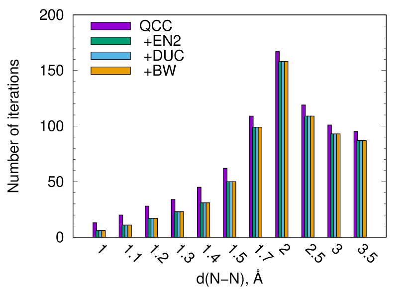
Figure 1: The number of iterations for the energy discrepancy $(E-E_{\text{FCI}})$ to fall below $0.1\text{\,}\mathrm{m\text{ $E_{\textup{ h }}$ }}$ as a function of $\ce{N-N}$ distance. Bare iQCC energies and their corrected by Eqs. (24), (30), and (36) counterparts labelled as “EN2”, “DUC”, and “BW”, respectively.

Figure 1 shows the number of iterations that are necessary to reduce the energy discrepancy $|E-E_{\text{FCI}}|$ below $0.1\text{\,}\mathrm{m\text{ $E_{\textup{ h }}$ }}$. It is remarkable that at the chosen level of accuracy all corrections require the same number of iterations. Near the equilibrium geometry, $\ce{d(N-N)}\approx$1.1\text{\,}\mathrm{\SIUnitSymbolAngstrom}$$, the corrections reduce the number of iterations by approximately a factor of 2 (e.g. at $\ce{d(N-N)}=$1.0\text{\,}\mathrm{\SIUnitSymbolAngstrom}$$ from 13 to 6). As the molecule is stretched, the efficiency of corrections deteriorates. This result is not unexpected since the perturbative treatment is inefficient in the strongly-correlated regime. Nevertheless, the practical utility of the corrections is still warranted as many experimental quantities, such as vibrational frequencies, etc. refer to near-equilibrium configurations.

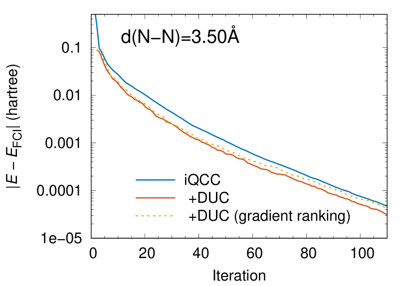
Figure 2: The absolute energy discrepancy $|E-E_{\text{FCI}}|$ as a function of iteration number for the bare iQCC energies and their corrected by Eq. (30) values. Solid lines correspond to the EN1-based generator ranking in the iQCC procedure, Eq. (37), while the short dashed line uses the original, gradient-based one.

We also assessed the EN-based generator ranking procedure [Eq. (37)]; see Fig. 2. As anticipated, the EN-based ranking is better than the original, gradient-based one, albeit marginally. Thus, we recommend the use of the former for highly stretched molecules or in other cases of strong correlation. Ranking by [Eq. (37)] has a negligible computational cost as the weights are free by-products of the energy corrections.

IV.3 Active-space treatment: The symmetric stretch of H2O

A symmetric water molecule stretch is another archetypal type of a strong correlation problem. We consider a water molecule with fixed $\angle\ce{HOH}=$107.6\text{\,}\mathrm{\SIUnitSymbolDegree}$$. When the 6-31G basis set is used and 1s core orbital of an O atom is frozen, the electronic Hamiltonian can be mapped to a 24-qubit operator. The size of the Hilbert space is $2^{24}\approx$1.7\text{\times}{10}^{7}$$, which makes the straightforward iQCC calculations difficult. We partition 24 qubits into two sets: the 8-qubit active one and the inactive set containing the remaining qubits. We employed the JW fermion-to-qubit transformation, in which it is easy to link the active qubit set with the fermionic (4,4) complete active space (CAS). CAS(4,4) consists of two pairs of orbitals which correlate at the dissociation limit . During QCC iterations only the generators with all-active indexes were ranked; four of them were included in the QCC ansatz for the next iteration. The convergence criterion was the same as for N2: the procedure was stopped when the absolute maximum gradient in the active set fell below 0.001.

The resulting potential energy curves for the active-space iQCC method and its corrected counterparts are shown in Fig. 3.

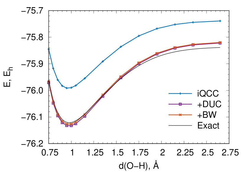
Figure 3: Potential energy curves for the symmetric H2O molecule stretch. The active-space qubit treatment, equivalent to CAS(4,4) embedded into the FCI (“exact”) problem (the Hartree–Fock orbital, which correlates with the 1s orbital of O is frozen) in the 6-31G basis.

As can be seen, all the corrections to the iQCC energies are large even at convergence, which is a hallmark of the approximate nature of the bare active-space iQCC energies. The mean deviations from the exact curve decrease from approximately $117\text{\,}\mathrm{m\text{ $E_{\textup{ h }}$ }}$ for the iQCC curve to $2.1\text{\,}\mathrm{m\text{ $E_{\textup{ h }}$ }}$ and $5.8\text{\,}\mathrm{m\text{ $E_{\textup{ h }}$ }}$ for DUC [Eq. (30)] and BW [Eq. (36)] corrections, respectively; see also Table 2.

Table 2: Various integral characteristics of curves in Fig. 3. All quantities are in $\mathrm{m\text{ $E_{\textup{ h }}$ }}$.

Method	Deviation, $(E-E_{\text{exact}})$			Non-parallelity
	Max	Min	Average
iQCC	$133.467\,383\,7$	$99.589\,832\,3$	$116.528\,608$	$33.877\,551\,4$
iQCC + DUC	$16.644\,271\,4$	$-12.442\,616$	$2.100\,827\,7$	$29.086\,887\,4$
iQCC + BW	$18.914\,101\,4$	$-7.295\,266\,4$	$5.809\,417\,5$	$26.209\,367\,8$

While small mean deviations are important for some quantities, such as singlet-triplet gaps, it is equally important to have curves that are almost parallel to the exact one, to predict properties like equilibrium geometries or vibrational frequencies, correctly. All the corrections decrease the non-parallelity (the difference between maximum and minimum deviations, see Table 2) for the whole considered region of O-H distances, from 0.75 to $2.65\text{\,}\mathrm{\SIUnitSymbolAngstrom}$. Moreover, both corrections drastically reduce the non-parallelity error for the region near the equilibrium geometry, $0.85\leq\ce{d(O-H)}\leq$1.15\text{\,}\mathrm{\SIUnitSymbolAngstrom}$$: from $15\text{\,}\mathrm{m\text{ $E_{\textup{ h }}$ }}$ to 4–$5\text{\,}\mathrm{m\text{ $E_{\textup{ h }}$ }}$. This result is consistent with the expectation that the perturbation theory-based corrections are more reliable when correlation is not too strong.

IV.4 T1–S0 gap in the Ir(ppy)3 complex

Encouraged by performance of the perturbative corrections near equilibrium configurations, we applied the enhanced iQCC method to a large, technologically relevant system, the tris-(2-phenylpyridine)iridium(III), Ir(ppy)3 complex; see Fig. 4.

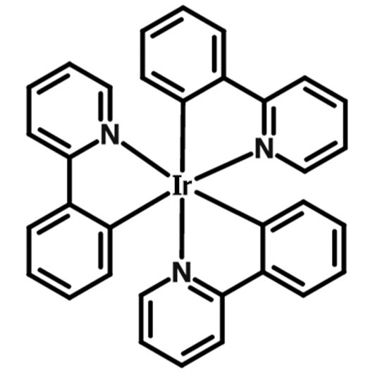
Figure 4: Tris-(2-phenylpyridine)iridium(III), Ir(ppy)3.

This molecule is probably the most studied green phosphorescent emitter Baldo et al. (1999, 2000); Holzer et al. (2005); Hofbeck and Yersin (2010) widely used in organic light-emitting diodes (OLEDs) Sun et al. (2006). Excited by recombination of electrons and holes injected from the corresponding transport layers, Ir(ppy)3 emits predominantly from the lowest triplet state (the singlet state is also bright) with almost 100% quantum efficiency. For the targeted design of similar and more advanced emitters it is important to reliably predict singlet-triplet gaps (in either singlet and triplet equilibrium geometries), but due to the size of molecules, the electronic-structure studies are typically limited to the density-functional theory (DFT) Jansson et al. (2007); Wu and Brédas (2008); Smith et al. (2011), with a prominent counterexample Kleinschmidt et al. (2015).

The ground singlet electronic state Ir(ppy)3 is reasonably well described by single-determinant Hartree–Fock or DFT methods. On the contrary, the triplet state is strongly multi-configurational with a multitude of closely-spaced energy levels that arise from population of low-lying d-orbitals of the Ir atom by an unpaired electron and its delocalization across the conjugated system. If the unrestricted Hartree–Fock method is used to describe the triplet state, the value of $\braket{\hat{S}^{2}}$ is approximately 5, deviating markedly from the ideal value of 2. Thus, the correct electronic structure is likely to be determined by a balance of orbital mixing and correlation effects, so that the CASSCF method may be the best choice for the problem; however, capturing dynamical correlation typically requires unrealistically large active spaces von Burg et al. (2020). Thus, the iQCC method augmented with corrections could be the best-suited method for such systems, since it accounts for the largest contributions variationally, while considering the bulk of small ones perturbatively allowing for the routine use of much larger active spaces.

To calculate the singlet-triplet gap we first optimized the molecular structure of ^3Ir(ppy)3 using the restricted open-shell Hartree–Fock (ROHF) method, which guarantees the spin purity of a Slater determinant. For the Ir atom we employed the 60-electron relativistic effective core pseudopotential (RECP) Stevens et al. (1992) with the partner double-zeta valence basis set as implemented in gamess, and the Pople split-valence double-zeta basis set augmented with polarization d orbitals for the second-row atoms C and N, 6-31G(d). With six-component d harmonics the atomic basis for the molecule contained $622$ functions. After the equilibrium geometry has been located, CAS (26e, 28o) has been created using 13 occupied and 15 unoccupied Hartree–Fock orbitals below and above the Fermi level, respectively. The electronic Hamiltonian corresponding to that CAS was generated and converted into the 56-qubit operator using the JW mapping and a pairwise grouping ($1\alpha$, $1\beta$, $2\alpha$, etc.) of spin-orbitals; the resulting Hamiltonian [Eq. (2)] contained $901\,985$ terms. A similar procedure was carried out for the singlet state in the same geometry: first, the restricted Hartree–Fock MOs were generated, then CAS(26e, 28o) was selected, and finally, the 56-qubit Hamiltonian was assembled from the values of one- and two-electron integrals in the chosen MO basis using the JW transformation resulting in $901\,973$-term operator.

We were able to perform 10 iQCC iterations using a single-generator QCC ansatz (5), results are shown in Table 3.

Table 3: Various estimates for the singlet-triplet gap for Ir(ppy)3.

Method	Singlet-triplet gap
	$\mathrm{eV}$	$\mathrm{nm}$
$\Delta$SCF(HF)	$2.95$	$421$
$\Delta$SCF(DFT/B3LYP)	$2.26$	$549$
$\Delta$MP2	$2.58$	$481$
iQCC(1 iter)	$=\Delta$SCF(HF)
iQCC(1 iter) + DUC	$2.57$	$483$
iQCC(5 iter)	$2.99$	$415$
iQCC(5 iter) + DUC	$2.56$	$485$
iQCC(10 iter)	$2.98$	$416$
iQCC(10 iter) + DUC	$2.54$	$488$
Exp.	$2.52$	$491$

It appears that the most of the correction to the $\Delta$SCF can be captured perturbatively, as both $\Delta$MP2 and “iQCC(1 iter) + DUC” results are already quite close to the reference value. The bare iQCC estimates behave non-monotonically, which is explained by slightly different rates of convergence of the absolute iQCC energies for singlet and triplet states. Corrected iQCC values (“+ DUC”), however, exhibit the monotonic convergence. Overall, the iQCC procedure converges slowly, and without perturbative corrections such a situation is detrimental for the iQCC method, as one would need to carry out prohibitively many iterations to reach the desired accuracy.

V Conclusions

We have developed and tested several numerical techniques that are aimed to a posteriori correct energies computed by the iQCC method. They are rooted in a new representation for qubit Hamiltonians, Eq. (9), in which regular and simple rules exist for evaluating matrix elements with the direct-product qubit states, Eqs. (11) and (12). In this respect it has a lot in common with normal-ordered fermionic Hamiltonians. The new decomposition naturally leads to a linear variational ansatz (20). Being not suitable for quantum computers, it allowed us to formulate the configuration interaction (CI)-like variational problem (21) and the qubit form of the second-order Epstein-Nesbet perturbation theory, Eq. (24); both can be efficiently evaluated on a classical computer.

Two essential modifications for the aforementioned techniques were also developed. The first is aimed to circumvent the divergence of the ENPT series due to small denominators in the strong correlation regime [see Eq. (30)]. The second is the unified variational-perturbational scheme, which “interpolates” between purely variational and perturbative solutions [see Sec. II.5] for flexible control of computational efforts. The unified scheme in the limit of a trivial $1\times 1$ effective Hamiltonian matrix reduces to the second-order Brillouin–Wigner perturbation theory.

Operationally, the new perturbative corrections require computing of a few extra quantities, namely, the mean-field excited energies [Eq. (23)]; everything else is available as elements of the original iQCC procedure. All these steps are not the computational bottleneck even for the largest problem considered here and can be safely offloaded to a classical computer. By capturing some of energy contributions classically, we additionally decrease the use of quantum resources. First of all, the total number of iQCC iterations is decreased for the same accuracy requirements. Secondly, by limiting the qubit indices of generators to be in the active set, we limit the growth of intermediate Hamiltonians and, thus, the number of quantum measurements needed at subsequent iterations.

Numerical assessment of the proposed techniques on several prototypical problems, namely, 10-qubit N2 dissociation, the 24-qubit symmetric water molecule stretch, and finally, and large-scale, 56-qubit simulations of the singlet-triplet gap in the Ir(ppy)3 complex have demonstrated a substantial improvement over the original iQCC method. New corrections address the most severe shortcoming of the original iQCC method: its numerical inefficiency in the case of weak correlation; they also provide additional flexibility in cases when only a subset of qubits is strongly correlated.

References

- Helgaker et al. (2000) T. Helgaker, P. Jorgensen, and J. Olsen, Molecular Electronic-structure Theory (Wiley, 2000).
- Preskill (2018) J. Preskill, Quantum 2, 79 (2018).
- Peruzzo et al. (2014) A. Peruzzo, J. McClean, P. Shadbolt, M.-H. Yung, X.-Q. Zhou, P. J. Love, A. Aspuru-Guzik, and J. L. O’Brien, Nat. Commun. 5, 4213 (2014).
- Wecker et al. (2015) D. Wecker, M. B. Hastings, and M. Troyer, Phys. Rev. A 92, 042303 (2015).
- Izmaylov et al. (2019) A. F. Izmaylov, T.-C. Yen, and I. G. Ryabinkin, Chem. Sci. 10, 3746 (2019), arXiv:1810.11602 [quant-ph] .
- Zhao et al. (2019) A. Zhao, A. Tranter, W. M. Kirby, S. F. Ung, A. Miyake, and P. Love, arXiv e-prints , 1908.08067 (2019).
- Huggins et al. (2019) W. J. Huggins, J. McClean, N. Rubin, Z. Jiang, N. Wiebe, K. B. Whaley, and R. Babbush, arXiv e-prints , arXiv:1907.13117 (2019), arXiv:1907.13117 [quant-ph] .
- Knill et al. (2007) E. Knill, G. Ortiz, and R. D. Somma, Phys. Rev. A 75, 012328 (2007).
- Izmaylov et al. (2020a) A. F. Izmaylov, T.-C. Yen, R. A. Lang, and V. Verteletskyi, J. Chem. Theory Comput. 16, 190 (2020a), arXiv:1907.09040 [quant-ph] .
- Yen et al. (2020) T.-C. Yen, V. Verteletskyi, and A. F. Izmaylov, J. Chem. Theory Comput. 16, 2400 (2020).
- Verteletskyi et al. (2020) V. Verteletskyi, T.-C. Yen, and A. F. Izmaylov, J. Chem. Phys. 152, 124114 (2020).
- Yen and Izmaylov (2020) T.-C. Yen and A. F. Izmaylov, arXiv e-prints (2020), arXiv:2007.01234 [quant-ph] .
- Nielsen and Chuang (2010) M. Nielsen and I. Chuang, Quantum Computation and Quantum Information: 10th Anniversary Edition (Cambridge University Press, 2010).
- Kandala et al. (2017) A. Kandala, A. Mezzacapo, K. Temme, M. Takita, M. Brink, J. M. Chow, and J. M. Gambetta, Nature 549, 242 (2017).
- Kandala et al. (2019) A. Kandala, K. Temme, A. D. Córcoles, A. Mezzacapo, J. M. Chow, and J. M. Gambetta, Nature 567, 491 (2019).
- McClean et al. (2016) J. R. McClean, J. Romero, R. Babbush, and A. Aspuru-Guzik, New J. Phys. 18, 023023 (2016).
- O’Malley et al. (2016) P. J. J. O’Malley, R. Babbush, I. D. Kivlichan, J. Romero, J. R. McClean, R. Barends, J. Kelly, P. Roushan, A. Tranter, N. Ding, B. Campbell, Y. Chen, Z. Chen, B. Chiaro, A. Dunsworth, A. G. Fowler, E. Jeffrey, E. Lucero, A. Megrant, J. Y. Mutus, M. Neeley, C. Neill, C. Quintana, D. Sank, A. Vainsencher, J. Wenner, T. C. White, P. V. Coveney, P. J. Love, H. Neven, A. Aspuru-Guzik, and J. M. Martinis, Phys. Rev. X 6, 031007 (2016).
- Romero et al. (2018) J. Romero, R. Babbush, J. R. McClean, C. Hempel, P. J. Love, and A. Aspuru-Guzik, Quantum Sci. Technol. 4, 014008 (2018).
- Hempel et al. (2018) C. Hempel, C. Maier, J. Romero, J. McClean, T. Monz, H. Shen, P. Jurcevic, B. P. Lanyon, P. Love, R. Babbush, A. Aspuru-Guzik, R. Blatt, and C. F. Roos, Phys. Rev. X 8, 031022 (2018).
- Nam et al. (2019) Y. Nam, J.-S. Chen, N. C. Pisenti, K. Wright, C. Delaney, D. Maslov, K. R. Brown, S. Allen, J. M. Amini, J. Apisdorf, K. M. Beck, A. Blinov, V. Chaplin, M. Chmielewski, C. Coleman, S. Debnath, A. M. Ducore, K. M. Hudek, M. Keesan, S. M. Kreikemeier, J. Mizrahi, P. Solomon, M. Williams, J. D. Wong-Campos, C. Monroe, and J. Kim, arXiv e-prints , 1902.10171 (2019), arXiv:1902.10171 .
- Lee et al. (2019) J. Lee, W. J. Huggins, M. Head-Gordon, and K. B. Whaley, J. Chem. Theory Comput. 15, 311 (2019).
- Evangelista et al. (2019) F. A. Evangelista, G. K.-L. Chan, and G. E. Scuseria, J. Chem. Phys. 151, 244112 (2019).
- Izmaylov et al. (2020b) A. F. Izmaylov, M. Díaz-Tinoco, and R. A. Lang, ArXiv e-prints , 2003.07351 (2020b), arXiv:2003.07351 [quant-ph] .
- Ryabinkin et al. (2018) I. G. Ryabinkin, T.-C. Yen, S. N. Genin, and A. F. Izmaylov, J. Chem. Theory Comput. 14, 6317 (2018), arXiv:1809.03827 [quant-ph] .
- Grimsley et al. (2019) H. R. Grimsley, S. E. Economou, E. Barnes, and N. J. Mayhall, Nat. Commun. 10, 3007 (2019), arXiv:1812.11173 [quant-ph] .
- Ryabinkin et al. (2020) I. G. Ryabinkin, R. A. Lang, S. N. Genin, and A. F. Izmaylov, J. Chem. Theory Comput. 16, 1055 (2020), pMID: 31935085, https://doi.org/10.1021/acs.jctc.9b01084 .
- McClean et al. (2018) J. R. McClean, S. Boixo, V. N. Smelyanskiy, R. Babbush, and H. Neven, Nat. Commun. 9, 4812 (2018).
- Lang et al. (2020) R. A. Lang, I. G. Ryabinkin, and A. F. Izmaylov, arXiv e-prints , arXiv:2002.05701 (2020), arXiv:2002.05701 [quant-ph] .
- Takeshita et al. (2020) T. Takeshita, N. C. Rubin, Z. Jiang, E. Lee, R. Babbush, and J. R. McClean, Phys. Rev. X 10, 011004 (2020).
-
Note (1)
Strictly speaking, the condition must be written as
where is a new generalized Ising Hamiltonian. It can be chosen arbitrarily, for example, to make the resulting generator commuting with global symmetry operators, such as the electron number or the total spin-squared ones. Additionally, this operator can be made unimodular, i.e. . - Epstein (1926) P. S. Epstein, Phys. Rev. 28, 695 (1926).
- Nesbet (1955) R. Nesbet, P. Roy. Soc. A - Math. Phy. 230, 312 (1955).
- Li and Evangelista (2019) C. Li and F. A. Evangelista, Annu. Rev. Phys. Chem. 70, 245 (2019), pMID: 30893000.
- Park et al. (2019) J. W. Park, R. Al-Saadon, N. E. Strand, and T. Shiozaki, J. Chem. Theory Comput. 15, 4088 (2019), pMID: 31244126.
- Assfeld et al. (1995) X. Assfeld, J. E. Almlöf, and D. G. Truhlar, Chem. Phys. Lett. 241, 438 (1995).
- Migani and Olivucci (2004) A. Migani and M. Olivucci, in Conical Intersection Electronic Structure, Dynamics and Spectroscopy, edited by W. Domcke, D. R. Yarkony, and H. Köppel (World Scientific, New Jersey, 2004) p. 271.
- Yarkony (1996) D. R. Yarkony, Rev. Mod. Phys. 68, 985 (1996).
- Löwdin (1963) P.-O. Löwdin, J. Mol. Spectrosc. 10, 12 (1963).
- Lennard-Jones and Fowler (1930) J. E. Lennard-Jones and R. H. Fowler, Proc. R. Soc. Lond. A 129, 598 (1930).
- Brillouin (1932) L. Brillouin, J. Phys. Radium 3, 373 (1932).
- Wigner (1997) E. P. Wigner, in Part I: Physical Chemistry. Part II: Solid State Physics (Springer Berlin Heidelberg, 1997) pp. 131–136.
- Nakano (1993) H. Nakano, Chem. Phys. Lett. 207, 372 (1993).
- Fales and Martinez (2020) B. S. Fales and T. J. Martinez, J. Chem. Theory Comput. 16, 1586 (2020), pMID: 31995369.
- Malrieu and Spiegelmann (1979) J. P. Malrieu and F. Spiegelmann, Theor. Chim. Acta 52, 55 (1979).
- Note (2) The occupied Hartree–Fock spin-orbitals and are mapped to single-qubit states and , respectively.
- Dunning (1989) T. H. Dunning, J. Chem. Phys. 90, 1007 (1989).
- Schmidt et al. (1993) M. W. Schmidt, K. K. Baldridge, J. A. Boatz, S. T. Elbert, M. S. Gordon, J. H. Jensen, S. Koseki, N. Matsunaga, K. A. Nguyen, S. J. Su, T. L. Windus, M. Dupuis, and J. Montgomery, J. Comput. Chem. 14, 1347 (1993).
- Gordon and Schmidt (2005) M. S. Gordon and M. W. Schmidt, in Theory and Applications of Computational Chemistry. The first forty years, edited by C. E. Dykstra, G. Frenking, K. S. Kim, and G. E. Scuseria (Elsevier, Amsterdam, 2005) pp. 1167–1189.
- Nielsen (2005) M. A. Nielsen, School of Physical Sciences The University of Queensland (2005).
- Note (3) We should mention that for the Hartree–Fock orbitals must be reordered.
- Baldo et al. (1999) M. A. Baldo, S. Lamansky, P. E. Burrows, M. E. Thompson, and S. R. Forrest, Appl. Phys. Lett. 75, 4 (1999).
- Baldo et al. (2000) M. A. Baldo, M. E. Thompson, and S. R. Forrest, Nature 403, 750 (2000).
- Holzer et al. (2005) W. Holzer, A. Penzkofer, and T. Tsuboi, Chem. Phys. 308, 93 (2005).
- Hofbeck and Yersin (2010) T. Hofbeck and H. Yersin, Inorg. Chem. 49, 9290 (2010).
- Sun et al. (2006) Y. Sun, N. C. Giebink, H. Kanno, B. Ma, M. E. Thompson, and S. R. Forrest, Nature 440, 908 (2006).
- Jansson et al. (2007) E. Jansson, B. Minaev, S. Schrader, and H. Ågren, Chem. Phys. 333, 157 (2007).
- Wu and Brédas (2008) Y. Wu and J.-L. Brédas, J. Chem. Phys. 129, 214305 (2008).
- Smith et al. (2011) A. R. G. Smith, P. L. Burn, and B. J. Powell, ChemPhysChem 12, 2429 (2011).
- Kleinschmidt et al. (2015) M. Kleinschmidt, C. van Wüllen, and C. M. Marian, J. Chem. Phys. 142, 094301 (2015).
- von Burg et al. (2020) V. von Burg, G. Hao Low, T. Häner, D. S. Steiger, M. Reiher, M. Roetteler, and M. Troyer, arXiv e-prints , arXiv:2007.14460 (2020), arXiv:2007.14460 [quant-ph] .
- Stevens et al. (1992) W. J. Stevens, M. Krauss, H. Basch, and P. G. Jasien, Can. J. Chem. 70, 612 (1992).
- Becke (1993) A. D. Becke, J. Chem. Phys. 98, 5648 (1993).
- Stephens et al. (1994) P. J. Stephens, F. J. Devlin, C. F. Chabalowski, and M. J. Frisch, J. Phys. Chem. 98, 11623 (1994).
- Sajoto et al. (2009) T. Sajoto, P. I. Djurovich, A. B. Tamayo, J. Oxgaard, W. A. Goddard, and M. E. Thompson, J. Am. Chem. Soc. 131, 9813 (2009).