Rydberg Magnetoexcitons in Cu₂O Quantum Wells

Abstract

We present theoretical approach that allows for calculation of optical functions for Cu₂O Quantum Well (QW) with Rydberg excitons in an external magnetic field of an arbitrary field strength. Both Faraday and Voigt configurations are considered, in the energetic region of p-excitons. We use the real density matrix approach and an effective e-h potential, which enable to derive analytical expressions for the QW magneto-optical functions. For both configurations, all three field regimes: weak, intermediate, and high field, are considered and treated separately. With the help of the developed approximeted method we are able to estimate the limits between the field regimes. The obtained theoretical magneto-absorption spectra show a good agreement with available experimental data.

I Introduction

The discovery of Rydberg excitons (REs) in cuprous oxide, first observed by Kazimierczuk et al Kazimierczuk initiated a large number of studies on their spectroscopic and optical properties, see the review paper AssmannBayer_2020 , where the extensive list of references can be found. A lot of attention has been devoted to the interaction of REs with an external electric and/or magnetic field (Stark and Zeeman effects) Refs.Rommel ^-Zielinska.PRB.2016.c and these phenomena have been studied, both experimentally and theoretically in bulk crystals or in plane-parallel slabs with dimensions much greater than the incident wave length and the effective Bohr radius. The exciton Rydberg energy in Cu₂O of about 90 meV is lower (regarding modulus) by the order of magnitude comparing with typical semiconductors (e.g., 4.2 meV in the prototypical semiconductor GaAs with n=3 as highest observed state). This reduction makes REs sensitive to external fields.

In low dimensional systems, due to confinement effects, the excitonic states have larger energy and oscillator strengths as compared to the bulk. This is also true for systems with REs; the states with large main quantum number gain additional energy therefore one can expect that depending on the type of confinement, new states can appear, originating from the overlapping of confinement states with the Coulomb states and eventually resulting from Zeeman splitting in an external magnetic field. Recently Cu₂O based nanostructures with REs have awoked an interest of several groups Ziemkiewicz_PRB_2020 ^,Naka ^-Konzelmann , because one can expects interesting quantum effects arising from competition between the geometric confinement, excitons motion and their interaction with additional external fields. The interest is also motivated by virtual benefits, because quantum-confined structures with REs might be of use in practice for costructing new class of optoelectronic aparatus. From practical point of view one has to mention that devices such as lasers, photodetectors, modulators, and switches based on quantum wells, turned out to be more faster then conventional electrical components, therefore they are desirable for technology and telecomunicatiom. It might be interesting to consider a possibility of an additional manipulation on demand by an external magnetic field applied to quantum wells with REs.

Similarly to the bulk case, an application of external fields to nanostructures changes the spectra of REs Ziemkiewicz_PRB_2020 . Since the electro- and magneto-optical properties of typical, the most studied case of GaAs based nanostructures have been explored for decades, the discussion of the Cu₂O, when multiple Rydberg exciton states must be taken into account, is already at the beginning. Here we will consider the effect of an external magnetic field on a quantum well with Rydberg excitons. The effects of a geometric confinement is superimposed on REs interaction with external fields, it manifests in intrinsic difference of magneto-optical spectra in terms of state energies, which in turn depend on a field orientation. Inspired by the recent development in the area of REs, we aim to analyze the magneto-optical properties of Cu₂O based quantum well (QW) in two diffrent field orientation, namely the Faraday and Voight configurations. Both cases have been investigated for bulk Cu₂O crystals with RE for weak magnetic field(up to 4 T) experimentally and the numerical excitonic spectra were shown Rommel .

We will use the real density matrix approach (RDMA) to calculate the optical functions of a single Cu₂O QW with REs. This approach turned out to be successful in describing the optical properties of Cu₂O bulk crystals, including effects of external fields Ref.Magnetoexcitons_2019 ^, Zielinska.PRB.2016.c ^,Zielinska.PRB.2016a . As it was shown in our recent paper Ziemkiewicz_PRB_2020 it is possible to extend the RDMA method for low dimensional systems. When describing the magneto-optical properties of the systems with excitons, one is confronted with well known difficulties. The exciton, being an analogy of a hydrogen atom, is created and maintained by a Coulomb attraction, having a spherical symmetry. On the other hand, in the case of a quantum well a magnetic field and the confinement potentials have a cylindrical symmetry. These geometrical discerepancies rule out an analytical solution of the proper Schrödinger equation for the problem. To circumvent such obstacles we have to use, as in the bulk case, various approximations, which depend on the relation between the exciton binding energy and the magnetic field energy. When the excitonic energies are larger than the magnetic field energies (the Landau states energies), we use the so-called weak field approximation. In the opposite case, when the Landau states energies are greater than the excitonic state energies we have to consider a high field approximation. Between these two regions one has to consider the intermediate field case, when both, the excitonic energies and the Landau state energies, are comparable. Moreover, each magnetic field regimes requires a different theoretical approach and there is strong need for a versatile estimation how to distinct the regime of the magnetic field; we propose the method, which allow to discern these regimes. When concerning the magneto-optical properties of excitons in a QW, one has to account for effects related to the direction of the applied magnetic field. One distinguishes between the Faraday configuration, when the magnetic field is directed along the growth axiss (the $z$-axis, perpendicular to the planes of the QW), and the Voigt configuration, when the magnetic field is perpendicular to the $z$-axis and parallel to the planes of the QW. We will show below, that all the above mentioned effects can be described within the RDMA.

The paper is organized as follows. In Sec. II we recall the basic equations of RDMA, adapted to the case of QWs, when external fields are applied. In the next three sections we explicitly derived the formulas for magneto-suscptibility for Cu₂O QWs when the external magnetic field is applied in the Faraday configuration. We separately discussed the cases of a week field (Sec. III.1), high field (Sec. III.2), and the intermediate magnetic field (Sec. III.3). Then we will also consider three different regimes of the magnetic field strength in the case of the Voigt configuration (Sections IV.1-IV.3). Sec. V contains illustrative numerical results and the description of a simple but effective method, which allows for estimation of the distintion between magnetic field regimes while a summary and conclusions of our paper are presented in Sec. VI. Four Appendices contain the details of analytical calculations.

II Basic equations

We will use the real density matrix approach, applied to single quantum well with Rydberg states, similary as it was done for low dimension structures in Ref. Ziemkiewicz_PRB_2020 In this approach the optical properties are described by an equation for the coherent amplitudes $Y_{12}$ of the electron-hole pair of coordinates ${\bf r}_{1}={\bf r}_{h}$ and ${\bf r}_{2}={\bf r}_{e}$ which for a pair of conduction and valence bands

$$-i(\hbar\partial_{t}+\Gamma)Y_{12}+H_{eh}Y_{12}={\bf M}{\bf E},$$ (1)

where ${\bf E}$ is the electric field, $\Gamma$ is a phenomenological damping coefficient, ${\bf M}(\textbf{r})$ is a smeared-out transition dipole density which depends on the coherence radius $r_{0}=\left[(2\mu/\hbar^{2})E_{g}\right]^{-1/2}$ and the $E_{g}$ is the fundamental gap; $\mu$ is reduced effective mass of the electron-hole pair and r is the relative electron-hole distance. Zielinska.PRB.2016a Specific forms of M(r) will be defined in subsequent sections.

RDMA, adopted for semiconductors by Stahl, Balslev, and others Stahl is a mesoscopic approach, which in the lowest order neglects all effects from the multiband semiconductor structure, so that the exciton Hamiltonian becomes identical to the two-band effective mass Hamiltonian $H_{eh}$, which in the case when external fields are applied, includes the electron and hole kinetic energy, the electron-hole interaction potential, the terms related to the external fields, and the confinement potentials.Hecktotter_2018 In consequence, the Hamiltonian $H_{eh}$ is given by

$$\phantom{nucl}H=E_{g}+\frac{1}{2m_{e}}\left({\bf p}_{e}-e\frac{{\bf r}_{e}\times{\bf B}}{2}\right)^{2}$$

$$+\frac{1}{2m_{h}}\left({\bf p}_{h}+e\frac{{\bf r}_{h}\times{\bf B}}{2}\right)_{z}^{2}$$

$$+\frac{1}{2m_{h}}\left({\bf p}_{h}+e\frac{{\bf r}_{h}\times{\bf B}}{2}\right)_{\parallel}^{2}+e{\bf F}\cdot({\bf r}_{e}-{\bf r}_{h})$$

$$+V_{\rm conf}({\bf r}_{e},{\bf r}_{h})-\frac{e^{2}}{4\pi\epsilon_{0}\epsilon_{b}|{\bf r}_{e}-{\bf r}_{h}|},$$ (2)

B is the magnetic field vector, ${\bf F}$ the electric field vector, $V_{\rm conf}$ are the surface potentials for electrons and holes, $m_{hz},m_{h\parallel}$ are the components of the hole effective mass tensor, and the electron mass is assumed to be isotropic. The total polarization of the medium is related to the coherent amplitude by

$${\bf P}({\bf R})=2\hbox{Re}\int d^{3}{r}\,{\bf M}({\bf r})Y({\bf R},{\bf r})$$ (3)

where R is the center-of-mass coordinate. This, in turn, is used in Maxwell’s field equation

$$c^{2}\nabla^{2}{\bf E(R)}-\epsilon_{b}\ddot{\bf E}=\frac{1}{\epsilon_{0}}{\bf\ddot{P}(R)}.$$ (4)

The excitonic susceptibility $\chi$ is then given by

$${\bf P(\omega,\textbf{k})}=\epsilon_{0}\chi(\omega,\textbf{k}){\bf E}(\omega,\textbf{k})$$ (5)

where $\omega$ is the frequency of the incident field and the absorption coefficient can be calculated from

$${\bf\alpha}=2\frac{\hbar\omega}{\hbar c}\hbox{Im}\,\sqrt{\epsilon_{b}+\chi},$$ (6)

where $\epsilon_{b}$ is the background dielectric constant. The detailed form of the Hamiltonian for both Faraday and Voigt configurations will be applied in the following sections.

III The Faraday configuration

When the magnetic field B is applied to a QW in the growth direction, which we identify with the $z$-axis, we deal with the Faraday configuration.

III.1 Weak field limit

In this configuration we will consider the optical response of the QW with thickness $L$ to a normally incident electromagnetic wave. The QW is located in the $x-y$ plane, with the surfaces at $z=\pm L/2$. We can separate the motion in the $z$-direction (where the particles are treated separately) from the in-plane motion where we use the relative- and exciton center-of-mass coordinates. In the case of $F=0$ we transform the Hamiltonian (II) into the form

$$H = H_{0}+\frac{P_{z}^{2}}{2M_{z}}+\frac{{\bf P}_{\parallel}^{2}}{2M_{\parallel}}+\frac{1}{8}\mu\omega_{c}^{2}r_{\parallel}^{2}+\frac{e}{2\mu^{\prime}}B{\mathcal{L}}_{z}$$ (7)

$$-\frac{e}{M_{\parallel}}{\bf P}_{\parallel}\cdot\left({\bf r}_{\parallel}\times{\bf B}\right)+V_{\rm conf}({\bf r}_{e},{\bf r}_{h}),$$

where $\omega_{c}={eB}/{\mu_{\parallel}}$ is the cyclotron frequency, the reduced mass $\mu^{\prime}$ is defined as

$$\frac{1}{\mu^{\prime}}=\frac{1}{m_{e}}-\frac{1}{m_{h}},$$ (8)

and $H_{0}$ is the two-band Hamiltonian for the relative electron-hole motion, as used in the papers. Zielinska.PRB ^, Zielinska.PRB.2016.b The operator ${\mathcal{L}}_{z}$ is the z-component of the angular momentum operator.

We assume a parabolic confinement in the $z$-direction,

$$V_{conf}=\frac{1}{2}m_{e}\omega_{ez}^{2}z_{e}^{2}+\frac{1}{2}m_{h}\omega_{hz}^{2}z_{h}^{2},$$ (9)

and using the notation

$$H^{(1D)}_{m,\omega}(z)=\frac{p_{z}^{2}}{2m}+\frac{1}{2}m\omega^{2}z^{2},$$ (10)

the QW Hamiltonian can be written in the form

$$H_{QW}=E_{g}+H_{m_{e},\omega_{ez}}^{(1D)}(z_{e})+H_{m_{h},\omega_{hz}}^{(1D)}(z_{h})$$

$$-\frac{\hbar^{2}}{2M_{z}}\partial^{2}_{Z}-\frac{\hbar^{2}}{2M_{\parallel}}\hbox{\boldmath$\nabla$}^{(2D)2}_{R_{\parallel}}-\frac{\hbar^{2}}{2\mu}\hbox{\boldmath$\nabla$}^{(2D)2}_{r}$$

$$-\frac{\mu}{\mu^{\prime}}{i}\gamma R^{*}\partial_{\phi}+\frac{R^{*}}{4a^{*2}}\gamma^{2}\,r^{2}+V_{eh},$$ (11)

where $V_{eh}$ is the electron-hole Coulomb interaction potential, $a^{*}$ is the exciton Bohr radius and $R^{*}$ the exciton Rydberg energy, $\hbox{\boldmath$\nabla$}^{(2D)2}_{R_{\parallel}},\hbox{\boldmath$\nabla$}^{(2D)2}_{r}$ denote 2-dimensional nabla operators, and $r=\sqrt{x^{2}+y^{2}}$. The dimensionless strength of the magnetic field $\gamma$ is defined as

$$\gamma=\hbar\omega_{c}/2R^{*},$$ (12)

In the weak magnetic field limit excitons play a dominant role in determining the optical response, the magnetic field can be treated as a perturbationMagnetoexcitons_2019 and we use the 2-dimensional Coulomb potential

$$V_{eh}=-\frac{e^{2}}{4\pi\epsilon_{0}\epsilon_{b}r}.$$ (13)

With respect to the above assumptions, the l.h.s. operator in Eq. (III.1) includes two one dimensional harmonic oscillator Hamiltonians and the 2-dimensional Coulomb Hamiltonian

$$H^{(2D)}_{Coulomb}=-\frac{\hbar^{2}}{2\mu}\hbox{\boldmath$\nabla$}^{(2D)2}_{r}-\frac{e^{2}}{4\pi\epsilon_{0}\epsilon_{b}r}.$$ (14)

We also neglect the terms related to the center-of-mass motion. Therefore the solution for the amplitude $Y$ can be expressed in terms of eigenfunctions of the mentioned Hamiltonians

$$Y_{jmN_{e}N_{h}}=$$ (15)

$$=\sum\limits_{N_{e},N_{h},j,m}c_{jmN_{e}N_{h}}\psi^{(1D)}_{\alpha_{ez,N_{e}}}(z_{e})\psi^{(1D)}_{\alpha_{hz,N_{h}}}(z_{h})\psi_{jm}(r,\phi),$$

where $\psi^{(1D)}_{\alpha_{z},N}(z)$ ($N_{e}$,$N_{h}$=0,1,…) are the quantum oscillator eigenfunctions for electron and hole, respectively.

$$\psi^{(1D)}_{\alpha_{z},N_{e,h}}(z)=\pi^{-1/4}\sqrt{\frac{\alpha_{z}}{2^{N}_{e,h}N_{e,h}!}}H_{N}(\alpha_{z}z)e^{-\frac{\alpha_{z}^{2}}{2}z^{2}},$$

$$\alpha_{z}=\sqrt{\frac{m_{e,h}\omega_{z}}{\hbar}},$$ (16)

$H_{N}(x)$ are Hermite polynomials $(N_{e,h}=0,1,\ldots)$, $m_{e,h}$ are the electron (hole) effective masses, and $\psi_{jm}(\rho,\phi)$ are the eigenfunctions of the 2-dimensional Hamiltonian (14)

$$\psi_{jm}(\rho,\phi)=R_{jm}(\rho)\frac{e^{im\phi}}{\sqrt{2\pi}},$$

$$R_{jm}=A_{jm}e^{-2\lambda\rho}(4\lambda\rho)^{|m|}L^{|2m|}_{j}(4\lambda\rho),$$ (17)

$$\lambda=\frac{1}{1+2(j+|m|)},$$

$$A_{jm}=\frac{4}{(2j+2|m|+1)^{3/2}}\left[\frac{j!}{(j+2|m|)!}\right]^{1/2},$$

where $L^{\alpha}_{n}(x)$ are the Laguerre polynomials, for which we use the definition

$$L^{\alpha}_{n}(x)={n+\alpha\choose n}M(-n,\alpha+1;x),$$

with the Kummer function $M(a,b,z)$ (the confluent hypergeometric function),Abramowitz , $\rho=r/a^{*}$ is the scaled space variable. Here we use the transition dipole density in the form Magnetoexcitons_2019

$$M(\hbox{\boldmath$\rho$},z_{e},z_{h})=\frac{M_{0}}{2\rho_{0}^{3}}\rho\,e^{-\rho/\rho_{0}}\frac{e^{i\phi}}{\sqrt{2\pi}}\delta(z_{e}-z_{h}),$$ (18)

with the integrated strength $M_{0}$ and the coherence radius $\rho_{0}=r_{0}/a^{*}$, where $r_{0}=\sqrt{\frac{\hbar^{2}}{2\mu E_{g}}}$. The coefficient $M_{0}$ and the coherence radius $\rho_{0}$ are connected through the longitudinal-transversal energy $\Delta_{LT}$ Zielinska.PRB.2016a

$$(M_{0}\rho_{0})^{2}=\frac{4}{3}\frac{\hbar^{2}}{2\mu}\epsilon_{0}\epsilon_{b}a^{*}\frac{\Delta_{LT}}{R^{*}}\,e^{-4\rho_{0}}.$$ (19)

The calculation of the QW susceptibility, from which other optical functions can be determined, consists of several steps. First, we assume that the incident electromagnetic wave is linearly polarized with the electric vector E with a component in the direction $\alpha$ and an amplitude $\mathcal{E}$; the dipole density vector M has a component $M$ in the form (18) in the same direction. Than, with the help od Eqs (3)and (5), applying the long wave approximation, we calculate the mean QW susceptibility from the formula

$$\chi=\frac{2}{\epsilon_{0}{\mathcal{E}}}\frac{1}{L}$$ (20)

$$\times\int\limits_{-L/2}^{L/2}dz_{e}dz_{h}\,d^{2}\hbox{\boldmath$\rho$}M(\hbox{\boldmath$\rho$},z_{e},z_{h})Y(\hbox{\boldmath$\rho$},z_{e},z_{h}).$$

The first step to calculate $\chi$ is to determine the exciton amplitude $Y$. Finally we use Eq. (1) with the Hamiltonian given by Eq. (III.1). Inserting the expansion (15) into Eq. (1) and making use of the dipole density in the form (18), one obtains a set of linear algebraic equations for the expansion coefficients $c_{jmN_{e}N_{h}}$

$$\sum_{\ell=0}^{j_{max}}a_{j\ell mN_{e}N_{h}}c_{\ell mN_{e}N_{h}}=b_{j1}\delta_{N_{e}N_{h}}{\mathcal{E}},$$

$$a_{j\ell mN_{e}N_{h}}=\delta_{j\ell}\kappa^{2}_{jmN_{e}N_{h}}+V_{j\ell m},$$

$$\kappa^{2}_{jmN_{e}N_{h}}=\frac{1}{R^{*}}\Biggl{(}E_{g}-\hbar\omega-i{\mit\Gamma}+\varepsilon_{jm}R^{*}+W_{eN_{e}}$$

$$+W_{hN_{h}}+\frac{\mu}{\mu^{\prime}}m\gamma\,R^{*}\Biggr{)},$$

$$\epsilon_{jm}=-4\lambda_{jm}^{2},$$

$$\lambda_{jm}=\frac{1}{2j+2|m|+1},$$ (21)

$$b_{j|m|N_{e}N_{h}}=b_{j1N_{e}N_{h}}$$

$$=\sqrt{\frac{(j+1)(j+2)}{(j+3/2)^{5}}}(1+2\rho_{0}\lambda_{j1})^{-4}F\left(-j,4;3;\frac{1}{s}\right)$$

$$s=\frac{1+2\rho_{0}\lambda_{jm}}{4\rho_{0}\lambda_{jm}},$$

$$j,\ell=0,1,2,\ldots,j_{max},\quad m=\pm 1,\quad N_{e},N_{h}=0,1,2,\ldots,$$

where $F(\alpha,\beta;\gamma;z)$ is a hypergeometric series. $V_{j\ell m}$ are matrix elements

$$V_{j\ell m}=\frac{1}{4}\gamma^{2}\langle R_{jm}(\rho)|\rho^{2}|R_{\ell m}(\rho)\rangle,$$ (22)

and their detailed form is given by Eq. (A) in Appendix A. The $z$-confinement energies $W_{eN_{e}},W_{hN_{h}}$ and the parameters $\alpha$ are defined as follows

$$\alpha_{e}=\sqrt{\frac{m_{e}}{\mu}}\sqrt{\frac{W_{e0}}{R^{*}}},$$

$$\alpha_{h}=\sqrt{\frac{m_{h}}{\mu}}\sqrt{\frac{W_{h0}}{R^{*}}},$$

$$p=\frac{1}{2}\left(\alpha_{ez}^{2}+\alpha_{hz}^{2}\right),$$

$$W_{e0}=\left(\frac{\pi a_{e}^{*}}{L}\right)^{2}R^{*}_{e},$$

$$W_{h0}=\left(\frac{\pi a_{h}^{*}}{L}\right)^{2}R^{*}_{h},$$

$$W_{e1}=3\,W_{e0},$$

$$W_{h1}=3\,W_{h0}.$$

For the case $\alpha_{e}=\alpha_{h}=\alpha^{F}=\pi/L$ the specific values of these parameters are

$$p=1,$$

$$W_{e0}=\left(\frac{\pi a_{e}^{*}}{L}\right)^{2}R^{*}_{e},$$

$$W_{h0}=\left(\frac{\pi a_{h}^{*}}{L}\right)^{2}R^{*}_{h},$$

$$\frac{W_{e0}+W_{h0}}{R^{*}}=\left(\frac{\pi a^{*}}{L}\right)^{2}=:\frac{W_{eh0}}{R^{*}},$$

$$\frac{W_{e1}+W_{h1}}{R^{*}}=\frac{3\,W_{eh0}}{R^{*}},$$

$$\frac{W_{eN}+W_{hN}}{R^{*}}=\frac{(2N+1)\,W_{eh0}}{R^{*}}.$$

With the above definitions, taking $N_{e}=N_{h}=N$ with computed $c$ coefficients, we use them in the expansion (15), which is in turn inserted into the Eq. (20), from which we calculate the mean QW magneto-susceptibility for the Faraday configuration

$$\chi^{F}(\omega)=48\epsilon_{b}\frac{\Delta_{LT}}{R^{*}}\left(\frac{a^{*}}{L}\right)$$

$$\times\sum_{j=0}^{\mathcal{N}}b_{j1}\left[\langle\Psi_{00}\rangle_{L}\left(c_{j100}+c_{j-100}\right)+\langle\Psi_{11}\rangle_{L}\left(c_{j111}+c_{j-111}\right)\right.$$

$$\left.+\ldots\langle\Psi_{NN}\rangle_{L}\left(c_{j1NN}+c_{j-1NN}\right)\right]$$ (23)

$$\langle\Psi_{NN}\rangle_{L}=\frac{1}{2^{N}\,N!}\frac{2}{\sqrt{\pi}}\int\limits_{0}^{\alpha L/2}e^{-t^{2}}H_{N}^{2}(t)dt.$$

III.2 High field limit

In the high field limit the magnetic energy contributions to the Hamiltonian are much greater then the Coulomb one and the energies of Landau states are larger than the absolute value of the lowest exciton state. Therefore we seek solutions for the exciton amplitude $Y$ in terms of the eigenfunctions of the "kinetic+magnetic+confinement " part of the Hamiltonian (III.1).

$$Y=\sum\limits_{nmN_{e}N_{h}}c_{nmN_{e}N_{h}}R_{nm}(\rho)\frac{e^{im\phi}}{\sqrt{2\pi}}\Psi_{N_{e}N_{h}}(z_{e},z_{h}),$$ (24)

where

$$R_{nm}(\rho)=$$ (25)

$$=\sqrt{\gamma}\sqrt{\frac{n!}{(n+|m|)!}}\left(\frac{\gamma\rho^{2}}{2}\right)^{|m|/2}e^{-\gamma\rho^{2}/4}L_{n}^{|m|}\left(\frac{\gamma\rho^{2}}{2}\right),$$

$n=0,1,\ldots$ and $m$ depict Landau states, $L_{n}^{|m|}$ are Laguerre polynomials. Similar as in the case of weak magnetic fields, we insert the expansion (24) into the Eq.(1) with an appropriate form of the Hamiltonian $H_{eh}$, to obtain the expansion coefficients $c$, which are calculated from the set of linear equations

$$\sum_{nmN_{e}N_{h}}a_{n\ell mN_{e}N_{h}}c_{nmN_{e}N_{h}}=d_{\ell m}\delta_{N_{e}N_{h}},$$

$$a_{n\ell mN_{e}N_{h}}=\delta_{n\ell}\kappa_{nmN_{e}N_{h}}^{2}+V_{n\ell m},$$ (26)

$$V_{n\ell m}=\langle R_{nm}|\left(-\frac{2}{\rho}\right)|R_{\ell m}\rangle,$$

$$d_{nm}=\langle R_{nm}\frac{e^{im\phi}}{\sqrt{2\pi}}|M(\rho,\phi)\rangle$$

$$=(M_{0}\rho_{0})\frac{2\gamma}{\sqrt{\pi}}\sqrt{n+1}\frac{\left(1-\frac{\gamma\rho_{0}^{2}}{2}\right)^{n}}{\left(1+\frac{\gamma\rho_{0}^{2}}{2}\right)^{n+2}}.$$

Here we have used the dipole density $M(\rho,\phi,z_{e},z_{h})$ in the form

$$M(\rho,\phi,z_{e},z_{h})=M_{0}\sqrt{\frac{2}{\pi}}\frac{\rho}{\rho_{0}^{3}}e^{-\rho^{2}/2\rho_{0}^{2}}\frac{e^{i\phi}+e^{-i\phi}}{\sqrt{2\pi}}\delta(z_{e}-z_{h}),$$ (27)

and

$$\kappa_{nmN_{e}N_{h}}^{2}=\frac{2\mu}{\hbar^{2}}a^{*2}(E_{g}-\hbar\omega-i{\mit\Gamma})$$

$$+U_{nm}/R^{*}+\frac{W_{eN_{e}}+W_{hN_{h}}}{R^{*}},$$ (28)

$$U_{nm}/R^{*}=\gamma\left(2n+\hbox{sgn}\,(B)\;m\frac{\mu}{\mu^{\prime}}+|m|+1\right).$$

The detailed form of the matrix elements $V_{n\ell m}$ is given by Eq. (65) in Appendix A. With the help of the coefficients $c$ one can get the exciton amplitude $Y$, which is then substitutes into Eq. (20), from which the mean magneto-susceptibility for the case of high magnetic fields can be determined. Restricting the considerations to the lowest confinement state in the $z$-direction and denoting $\kappa_{nm00}=\kappa_{nm}$, the magneto-susceptibility for the Faraday configuration for the high field is given by the follwing formula

$$\chi^{F}=\frac{16}{3\pi}\epsilon_{b}\gamma^{2}\left(\frac{a^{*}}{L}\right)\frac{\Delta_{LT}}{R^{*}}e^{4\rho_{0}}\,\frac{\alpha_{e}\alpha_{h}}{p}$$

$$\times\hbox{erf}\,\left(\frac{L\sqrt{p}}{2}\right)\sum\limits_{n=0}^{N}\sum_{m}\,c_{nm}d_{n1},$$

$$d_{n1}=\sqrt{n+1}\exp[2\rho_{0}-(n+1)\gamma\rho_{0}^{2}],$$ (29)

$$\sum\limits_{n=0}^{n_{max}}a_{n\ell\,m}c_{nm}=d_{\ell\,1},$$

$$a_{n\ell m}=\delta_{n\ell}\kappa_{nm}^{2}+V_{n\ell},$$

$$\kappa_{nm}^{2}=\frac{E_{g}-\hbar\omega-i{\mit\Gamma}+U_{nm}+W_{e0}+W_{h0}}{R^{*}}.$$

III.3 Intermediate fields

For intermediate magnetic fields the exciton energies and the Landau states energies are comparable, therefore we must include the contributions from Coulomb interaction and the magnetic field at the same footing. In Ref. Magnetoexcitons_2019 we have developed the method for such calculations and here we will recall its fundamental points. The Eq. (1) has to be transformed into a Lippmann-Schwinger equation

$$H_{kin+B+confinement}Y=ME-VY,$$ (30)

where $V$ is the 2-dimensional Coulomb e-h interaction potential, and $H_{kin+B+confinement}$ is the "kinetic+magnetic+confinement¨part of the Hamiltonian (7). The above equation can be solved by means of an appropriate Green’s function Mott

$$Y=GME-GVY.$$ (31)

The Green function has the form Mott

$$G(\rho,\rho^{\prime};\phi,\phi^{\prime};z_{e},z_{e}^{\prime};z_{h},z_{h}^{\prime})=$$

$$=\frac{1}{2\pi}\sum\limits_{N_{e}.N_{h}}\sum\limits_{n=0}^{\infty}\sum_{m}e^{im(\phi-\phi^{\prime})}\psi^{(1D)}_{\alpha_{h},N_{h}}(z_{h})\psi^{(1D)}_{\alpha_{h},N_{h}}(z_{h}^{\prime})$$

$$\times\psi^{(1D)}_{\alpha_{e},N_{e}}(z_{e})\psi^{(1D)}_{\alpha_{e},N_{e}h}(z_{e}^{\prime})\frac{R_{nm}(\rho)R_{nm}(\rho^{\prime})}{\kappa_{nmN_{e}N_{h}}^{2}},$$

where $R_{nm}(\rho)$ are given in Eq. (25), and $\kappa_{nmN_{e}N_{h}}^{2}$ is given by Eq. (III.2).

The Lippmann-Schwinger equation (30) is an integral equation for the unknown function $Y$. There are several methods to solve such equations. We choose the method of an trial function $Y$, which we take in the form

$$Y=\Psi_{00}R_{01}(\rho)\left[\sum\limits_{m=\pm 1}Y_{0m,00}\exp(-\kappa_{0m00}\rho)\frac{e^{im\phi}}{\sqrt{2\pi}}\right]$$

$$+\sum\limits_{n=1}^{\infty}\sum\limits_{N_{e},N_{h}\geq 1}\sum\limits_{m}\frac{e^{im\phi}}{\sqrt{2\pi}}Y_{nmN_{e}N_{h}}R_{nm}(\rho)\Psi_{N_{e}N_{h}},$$ (32)

where $Y_{nmN_{e}N_{h}}$ are coefficients to be determined, and

$$\Psi_{N_{e}N_{h}}=\psi^{(1D)}_{\alpha_{e},N_{e}}(z_{e})\psi^{(1D)}_{\alpha_{h},N_{h}}(z_{h}).$$ (33)

The exciton amplitude $Y$, and thus the magneto-susceptibility, is known once the parameters $Y_{nmN_{e}N_{h}}$ are calculated. The method of calculation is given in Appendix B, where we obtained

$$Y_{0\pm 1,00}=\frac{2\mu}{\hbar^{2}a^{*}}\left[(M_{0}\rho_{0})\frac{2\gamma}{\sqrt{\pi}}\right]{\mathcal{E}}$$

$$\times\frac{d_{01}e^{-z^{2}/4}}{3\kappa_{0\pm 1,00}^{2}D_{-4}(z)-2\sqrt{\gamma}D_{-3}(z)},$$ (34)

where $D_{\nu}(z)$ are parabolic cylinder functions,Grad

$$z=\frac{\kappa_{0\pm 1,00}}{\sqrt{\gamma}},$$

and

$$Y_{n\pm 1,00}=\frac{2\mu}{\hbar^{2}a^{*}}\left[(M_{0}\rho_{0})\frac{2\gamma}{\sqrt{\pi}}\right]{\mathcal{E}}\frac{d_{n1}}{\kappa^{2}_{0\pm 1,00}}.$$ (35)

With the above quantities, substituted in Eq. (III.3) and Eq. (20), we obtained the mean QW magneto-susceptibility in the Faraday configuration and intermediate magnetic field regime in the form

$$\chi=\frac{16}{3\pi}\epsilon_{b}\gamma^{2}\left(\frac{a^{*}}{L}\right)\frac{\Delta_{LT}}{R^{*}}e^{4\rho_{0}}\frac{\alpha_{e}\alpha_{h}}{p}\hbox{erf}\,\left(\frac{L\sqrt{p}}{2}\right)$$

$$\times\sum_{m=\pm 1}\Biggl{\{}\frac{3d_{0m}\exp\left(\frac{u^{2}}{4}\right)D_{-4}(u)}{\exp(z^{2}/4)\left[3\kappa_{0m}^{2}D_{-4}(z)-2\sqrt{\gamma}D_{-3}(z)\right]}$$

$$+\sum\limits_{n=1}^{N}\frac{d_{nm}^{2}}{\kappa_{nm}^{2}}\Biggr{\}},$$ (36)

$$d_{nm}=d_{n|m|}=\sqrt{n+1}\frac{(1-\gamma\rho_{0}^{2}/2)^{n}}{(1+\gamma\rho_{0}^{2}/2)^{n+2}}$$

$$\approx\sqrt{n+1}\;e^{-(n+1)\gamma\rho_{0}^{2}},$$

$$u=\frac{\kappa_{0\pm 1}}{s},\quad s=\frac{1}{\rho_{0}}\left(1+\frac{\gamma\rho_{0}^{2}}{2}\right)^{1/2},\;z=\frac{\kappa_{0\pm 1}}{\sqrt{\gamma}}.$$

IV The Voigt configuration

In the Voigt configuration the magnetic field is perpendicular to the wave vector of the propagating electromagnetic wave and, in the QW geometry, parallel to the QW planes.

IV.1 Weak field regime

We choose the magnetic field B parallel to the $0x$-axis, which corresponds to the vector potential

$$\textbf{A}=\frac{B}{2}(0,-z,y).$$ (37)

With this potential and the confinement potentials (9), the QW Hamiltonian (II) takes the form

$$H^{V}_{\rm QW}=E_{g}+\frac{1}{2m_{e}}p_{ex}^{2}+\frac{1}{2m_{h}}p_{hx}^{2}$$

$$+\frac{1}{2m_{e}}p_{ey}^{2}+\frac{1}{2m_{h}}p_{hy}^{2}+\frac{1}{8m_{e}}e^{2}B^{2}y_{e}^{2}+\frac{1}{8m_{h}}e^{2}B^{2}y_{h}^{2}$$

$$-\frac{1}{2m_{e}}p_{ey}eBz_{e}+\frac{1}{2m_{h}}p_{hy}eBz_{h}$$ (38)

$$+\frac{1}{2m_{e}}p_{ez}^{2}+\frac{1}{8m_{e}}e^{2}B^{2}z_{e}^{2}+\frac{1}{2}m_{e}\omega_{ez}^{2}z_{e}^{2}$$

$$+\frac{1}{2m_{h}}p_{hz}^{2}+\frac{1}{2}m_{hz}\omega_{hz}^{2}z_{h}^{2}+\frac{1}{8m_{h}}e^{2}B^{2}z_{h}^{2}$$

$$+p_{ez}eBy_{e}-p_{hz}eBy_{h}$$

$$-\frac{e^{2}}{4\pi\epsilon_{0}\epsilon_{b}}\left[\left(x_{e}-x_{h}\right)^{2}+\left(y_{e}-y_{h}\right)^{2}\right]^{-1/2}.$$

As in the case of the Faraday configuration, we will discuss the three regimes: weak, intermediate and the high magnetic field with the proper form of the Hamiltonian for each of them.

In the weak field limit we transform the Hamiltonian (IV.1) to the form

$$H^{V}_{\rm QW}=E_{g}+\frac{1}{2m_{e}}p_{ex}^{2}+\frac{1}{2m_{e}}p_{ey}^{2}$$

$$-\frac{e^{2}}{4\pi\epsilon_{0}\epsilon_{b}}\left[\left(x_{e}-x_{h}\right)^{2}+\left(y_{e}-y_{h}\right)^{2}\right]^{-1/2}$$

$$+\frac{1}{2m_{e}}p_{ez}^{2}+\frac{1}{2}m_{e}\Omega_{ez}^{2}+\frac{1}{2m_{h}}p_{hz}^{2}+\frac{1}{2}m_{h}\Omega_{hz}^{2}+H^{\prime},$$

$$\Omega_{ez}^{2}=\frac{\omega_{ec}^{2}}{4}+\omega_{ez}^{2},\quad\omega_{ec}=\frac{eB}{m_{e}},$$ (39)

$$\Omega_{hz}^{2}=\frac{\omega_{hc}^{2}}{4}+\omega_{hz}^{2},\quad\omega_{hc}=\frac{eB}{m_{h}},$$

$$H^{\prime}=\frac{1}{8m_{e}}e^{2}B^{2}y_{e}^{2}+\frac{1}{8m_{h}}e^{2}B^{2}y_{h}^{2}.$$

Introducing the relative and the center-of-mass coordinates $y,M_{Y}$ in the $y$ direction

$$M_{Y}=\frac{m_{e}y_{e}+m_{h}y_{h}}{M},\quad y=y_{e}-y_{h},\qquad M=m_{e}+m_{h}$$

we transform the Hamiltonian (IV.1) to the form

$$H^{V}_{\rm QW}=E_{g}+H^{(2D)}_{Coul}+H^{(1D)}_{m_{e},\Omega_{ez}}\left(z_{e}\right)+H^{(1D)}_{m_{h},\Omega_{hz}}\left(z_{h}\right)+H^{\prime},$$

$$H^{\prime}=\frac{1}{8\mu}e^{2}B^{2}M_{Y}^{2}+\frac{1}{8\mu}e^{2}B^{2}y^{2}q+\frac{1}{4\mu^{\prime}}e^{2}B^{2}M_{Y}y,$$ (40)

$$q=\frac{m_{h}^{2}-m_{h}m_{e}+m_{e}^{2}}{M^{2}}.$$

We will proceed in a similar way as in the case of a weak field in the Faraday configuration. Treating the magnetic part $H^{\prime}$ as a perturbation, we assume the solution for $Y$ in the form (15), with the eigenfunctions appropriate to the Hamiltonian (IV.1). This leads to the system of equations (III.1) for the expansion coefficients $c$, where now the matrix elements are given by

$$V^{Voigt}_{jkm}=\frac{1}{2}q\,V^{Faraday}_{jkm},$$ (41)

with $V^{Faraday}_{jkm}$ defined in Eq. (A).

The susceptibility is obtained in the form (III.1), where

$$\langle\Psi_{NN}\rangle_{L}=\frac{1}{2^{N}\,N!}\frac{2}{\sqrt{\pi}}\int\limits_{0}^{\alpha^{V}L/2}e^{-t^{2}}H_{N}^{2}(t)dt,$$ (42)

$$\alpha_{e}^{V}=\alpha_{h}^{V}=:\alpha^{V}=\frac{1}{a^{*}}\left[\frac{\gamma^{2}}{4}+\left(\frac{\pi a^{*}}{L}\right)^{4}\right]^{1/4},$$

$$\frac{W_{e0}^{V}}{R^{*}}+\frac{W_{h0}^{V}}{R^{*}}=\frac{W^{V}_{eh0}}{R^{*}}=\left[\frac{\gamma^{2}}{4}+\left(\frac{\pi a^{*}}{L}\right)^{4}\right]^{1/2},$$

and, for $N_{e}=N_{h}=N$, the confinement energies are now defined as

$$W^{V}_{eN}+W^{V}_{hN}=W_{NN}=(2N+1)W^{V}_{eh0},$$

$$N=0,1,2,\ldots,N_{max},$$ (43)

$$W^{V}_{eh0}=\left[\frac{\gamma^{2}}{4}+\left(\frac{\pi a^{*}}{L}\right)^{4}\right]^{1/2}R^{*}.$$

IV.2 High field regime

In the high field limit for the Voigt configuration the e-h Coulomb interaction is considered as a perturbation, so the unperturbed QW Hamiltonian has the form

$$H^{V}_{QW}=\frac{p_{x}^{2}}{2\mu}+H^{(1D)}_{\mu,\Omega_{y}}(y)+H^{(1D)}_{m_{e},\Omega{ez}}(z_{e})+H_{m_{h},\Omega_{hz}}(z_{h}),$$

$$\frac{\hbar\Omega_{y}}{2R^{*}}=\frac{\gamma}{2}\sqrt{q},$$ (44)

with $q$ defined in Eq.(IV.1). We apply the method of the so called adiabatic potentials, used in bulk crystals (seeMagnetoexcitons_2019 and references therein), here adapted for the case of QWs. The exciton amplitude $Y$ will be assumed in the form

$$Y(x,y,z_{e},z_{h})$$ (45)

$$=\sum\limits_{N_{x}N_{y}N_{e}N_{h}}c_{N_{x}N_{y}N_{e}N_{h}}\psi_{N_{x}}(x)\psi^{(1D)}_{\beta,\Omega_{y}}(y)\Psi_{N_{e}N_{h}}(z_{e},z_{h}),$$

where

$$\psi^{(1D)}_{\beta,N_{y}}=\pi^{-1/4}\sqrt{\frac{\beta}{2^{N_{y}}N_{y}!}}H_{N_{y}}(\beta y)e^{-\beta^{2}y^{2}/2},$$

$$\beta=\frac{1}{a^{*}}\sqrt{\frac{\hbar\Omega_{y}}{2R^{*}}}=\frac{1}{a^{*}}\,q^{1/4}\sqrt{\frac{\gamma}{2}}=\frac{1}{a^{*}}\tilde{\beta},$$ (46)

$$\Psi_{N_{e}N_{h}}(z_{e},z_{h})=\psi^{(1D)}_{\alpha_{e}^{V},N_{e}}(z_{e})\psi^{(1D)}_{\alpha_{h}^{V},N_{e}}(z_{h}),$$

and $\psi_{N_{x}}(x)$ are eigenfunctions of the operator

$$H_{x}=\frac{p_{x}^{2}}{2\mu}+V_{N_{y}N_{y}^{\prime}}(x),$$ (47)

where

$$V_{N_{y}N_{y}^{\prime}}(x)=-2\int\limits_{-\infty}^{\infty}dy\frac{\psi^{(1D)}_{\beta,N_{y}}(y)\psi^{(1D)}_{\beta,N^{\prime}_{y}}(y)}{\sqrt{x^{2}+y^{2}}}.$$ (48)

We restrict the discussion to the diagonal terms $V_{N_{y}N_{y}}$, and approximate the expression (48) by

$$V_{N_{y}}=-\frac{2}{a_{N_{y}}+|x|}.$$ (49)

The coefficients $a_{N_{y}}$, for odd parity eigenfunctions $\psi^{(1D)}_{\beta,N_{y}},\;N_{y}=2n+1$, are calculated in Appendix C. In this approximation the Schrödinger equation with the operator (47) becomes

$$\left(\frac{p_{x}^{2}}{2\mu}-\frac{2}{a_{N_{y}}+|x|}\right)\psi=E\psi,$$ (50)

which gives the eigenfunctions

$$\psi_{jn}(x)=\frac{\sqrt{2}}{j+1}e^{-(|x|+a_{2n+1})/(j+1)}L^{1}_{j}\left[\frac{2(|x|+a_{2n+1})}{j+1}\right],$$ (51)

$j=0,1,\ldots,$ and eigenvalues

$$E_{j}=-\frac{R^{*}}{(j+1)^{2}}.$$ (52)

Having the above functions, and using the dipole density in the form

$$M(x,y,z_{e},z_{h})$$ (53)

$$=\frac{M_{0}}{2\rho_{0}^{3}}\sqrt{\frac{2}{\pi}}e^{-\frac{x^{2}}{2\rho_{0}^{2}}}y\,e^{-\frac{y^{2}}{2\rho_{0}^{2}}}\delta(z_{e}-z_{h}),$$

we calculate the expansion coefficients in the formula Eq. (45) and thus the exciton amplitude $Y$ and, finally, the mean QW magneto-susceptibility for the Voigt configuration in the limit of high magnetic fields

$$\chi^{V}=\frac{4\sqrt{\pi}}{3}\epsilon_{b}\Delta_{LT}e^{4\rho_{0}}\sum\limits_{j=0}^{N_{x}max}\sum\limits_{n=0}^{N_{y}max}\sum\limits_{N=0}^{N_{z}max}\frac{2}{(j+1)^{2}}\,$$

$$\times\,e^{-\frac{2a_{2n+1}}{j+1}}\left[L_{j}^{(1)}\left(\frac{2\,a_{2n+1}}{j+1}\right)\right]^{2}$$ (54)

$$\times\left(\frac{2\tilde{\beta}}{1+\tilde{\beta}^{2}\rho_{0}^{2}}\right)^{3}\frac{(2n+1)!}{2^{2n+1}(n!)^{2}}\left(\frac{1-\tilde{\beta}^{2}\rho_{0}^{2}}{1+\tilde{\beta}^{2}\rho_{0}^{2}}\right)^{2n}$$

$$\times\left[E_{g}-\hbar\omega-\frac{R^{*}}{(j+1)^{2}}+\left(2n+\frac{3}{2}\right)\hbar\Omega_{y}+W_{NN}\right]^{-1},$$

where $\langle\Psi_{NN}\rangle_{L}$ are defined in Eq. (42), and the confinement energies $W_{NN}$ in Eq. (IV.1).

IV.3 Intermediate fields

We calculate the mean magneto-susceptibility for the Voigt configuration and in the regime of intermediate magnetic fields by the Green function method described above for the case of Faraday configuration. Again, we use the Lippmann-Schwinger equation (31) to calculate the exciton amplitude $Y$, which is then used to obtain the magneto-susceptibility. The Green’s function in Eq. (31) satisfies, by definition, the equation

$$H^{V}G(x,x^{\prime};y,y^{\prime};z_{e},z_{e}^{\prime};z_{h},z_{h}^{\prime})$$

$$=-\delta(x-x^{\prime})\delta(y-y^{\prime})\delta(z_{e}-z_{e}^{\prime})\delta(z_{h}-z_{h}^{\prime})$$

where the operator $H^{V}$ has the form (IV.2). Expressing Green’s function in terms of eigenfunctions of the operators contained in $H^{V}$ one obtains

$$G=\frac{2\mu}{\hbar^{2}}\sum\limits_{n,N_{e},N_{h}}{\frac{1}{2\pi}}\int\limits_{-\infty}^{\infty}dk\,e^{ik(x-x^{\prime})}\psi^{(1D)}_{\beta,n}(y)\psi^{(1D)}_{\beta,n}(y^{\prime})$$

$$\times\frac{\psi^{(1D)}_{\alpha_{e}^{V},N_{e}}(z_{e})\psi^{(1D)}_{\alpha_{e}^{V},N_{e}}(z_{e}^{\prime})\psi^{(1D)}_{\alpha_{h}^{V},N_{h}}(z_{h})\psi^{(1D)}_{\alpha_{h}^{V},N_{h}}(z^{\prime}_{h})}{k^{2}+\kappa_{nN_{e}N_{h}}^{2}}$$ (55)

with

$$\kappa_{nN_{e}N_{h}}^{2}=\frac{2\mu}{\hbar^{2}}\Biggl{[}(E_{g}-\hbar\omega-i{\mit\Gamma})$$ (56)

$$+\left(2n+\frac{3}{2}\right)\hbar\Omega_{y}+\left(N_{e}+\frac{1}{2}\right)\hbar\Omega_{ez}+\left(N_{h}+\frac{1}{2}\right)\hbar\Omega_{hz}\Biggr{]}.$$

The functions $\psi^{(1D)}_{\beta,n}(y)$ are defined in Eq. (IV.2). For the further calculations we must specify a trial function $Y$. Accounting only the lowest confinement state we use the following trial function of the form

$$Y=Y_{0}\Psi_{00}\psi_{1,\beta}^{(1D)}(y)e^{-\kappa_{0}\sqrt{x^{2}+y^{2}}}$$ (57)

$$+\sum\limits_{n=1}^{\infty}\sum\limits_{N_{e}N_{h}\geq 1}\psi_{2n+1,\beta}^{(1D)}(y)\Psi_{N_{e}N_{h}}\frac{1}{2\pi}\int\limits_{-\infty}^{\infty}dk\,Y_{nN_{e}N_{h}}(k)e^{ikx},$$

where $\kappa_{0}^{2}=\kappa_{000}^{2}$, $Y_{0},Y_{nN_{e}N_{h}}$ $\Psi_{N_{e}N_{h}}$ is defined in Eq. (IV.2) and coefficients have to be determined; the detailed calculations are presented in Appendix D. With the help of these the coefficients determined the the exciton amplitude and than, similary as in the section III C one can calculate the mean magneto-susceptibility for the Voigt configuration and in the intermediate field regime, arriving to the formula

$$\chi^{intermV}=$$

$$=\frac{4}{3}\frac{\Delta_{LT}}{R^{*}}\epsilon_{b}\left(\frac{a^{*}}{L}\right)\langle\Psi_{00}\rangle_{L}\Biggl{\{}\frac{1}{\sqrt{\pi}\kappa_{0}}\rho_{0}^{3}\left(\frac{2\beta}{1+\beta^{2}\rho_{0}^{2}}\right)^{3}$$

$$\times\exp\left[\frac{\kappa_{0}^{2}\rho_{0}^{2}}{4(1+\beta^{2}\rho_{0}^{2})}\right]D_{-3}\left(\frac{\kappa_{0}\rho_{0}}{\sqrt{1+\beta^{2}\rho_{0}^{2}}}\right)$$

$$\times\left[\frac{2^{3/2}}{\sqrt{\pi}}e^{\kappa_{0}^{2}/8\beta^{2}}D_{-3}\left(\frac{\kappa_{0}}{\beta\sqrt{2}}\right)-F(\kappa_{0},\beta)\right]^{-1}$$

$$+\sum\limits_{n\geq 1,N\geq 1}\Biggl{\{}\langle\Psi_{NN}\rangle_{L}\frac{1}{2^{2n}}$$ (58)

$$\times\left(\frac{\tilde{\beta}}{1+\tilde{\beta}^{2}\rho_{0}^{2}}\right)^{3}\frac{(2n+1)!}{(n!)^{2}}\left(\frac{\tilde{\beta}^{2}\rho_{0}^{2}-1}{\tilde{\beta}^{2}\rho_{0}^{2}+1}\right)^{2n}\frac{\pi}{\kappa_{nN}}w(i\beta\,\kappa_{nN})\Biggr{\}},$$

$W_{\kappa,\mu}(z)$ is Whittaker’s function of the second kind, $w(z)$ is the complex error function,Abramowitz and $F(\kappa_{0},\beta)$ is defined in Eq. (D).

Table 1: Band parameter values for Cu₂O, masses in free electron mass $m_{0}$, $R^{*}$ calculated from $(\mu/\epsilon_{b}^{2})\cdot 13600\,\hbox{meV}$,  $R^{*}_{e,h}=(m_{e,h}/\mu)R^{*},a^{*}_{e,h}=(\mu/m_{e,h})a^{*}$

Parameter	Value	Unit	Reference
$E_{g}$	2172.08	meV	Kazimierczuk
$R^{*}$	87.78	meV
$\Delta_{LT}$	$1.25\times 10^{-3}$	meV	Stolz
$m_{e}$	0.99	$m_{0}$	Naka
$m_{h}$	0.58	$m_{0}$	Naka
$\mu$	0.363	$m_{0}$
$M_{tot}$	1.56	$m_{0}$
$a^{*}$	1.1	nm	Kazimierczuk
$r_{0}$	0.22	nm	Zielinska.PRB
$\epsilon_{b}$	7.5		Kazimierczuk
${R_{e}^{*}}$	239.4	meV
${R^{*}_{h}}$	140.25	meV
${a^{*}_{e}}$	0.4	nm
${a^{*}_{h}}$	0.69	nm
$\Gamma_{j}$	3.88/$j^{3}$	meV	Kazimierczuk ; maser2

V Results of specific calculations

We have calculated the QW magneto-absorption from the imaginary part of the magneto-susceptibilities, given for the Faraday configuration in equations (III.1), (III.2), (III.3), and for the Voigt configuration in equations (III.1) (with adequate change of parameters), (IV.2), and (IV.3). The parameters used in calculations are collected in Table 1. We assume that the QW band parameters (for example, effective masses), are equal to their bulk values. Since the quantum well thickness under consideration is $L\geq 20$ nm, it is much larger than the exciton (1.1 nm for n=1, see RefKazimierczuk ), the choice of bulk effective masses is justified. The calculations have been performed for the whole magnetic field strength spectrum, including the weak, intermediate, and high field regimes.

V.1 Estimation of regime boundaries

The problem of delimiting boundaries of magnetic fields regimes requires specific analysis for each material. Below we will present a heuristic and simple method, which allows for rough estimation of these limits. The lowest Landau energies for p-exciton (including the Zeeman splitting) given by (see (Eq. III.2))

$$U_{0,\pm 1}=\left(\frac{B}{B_{cr}}\right)\left(2\pm\frac{\mu}{\mu^{\prime}}\right)R^{*},$$ (59)

are compared to the 2-dimensional hydrogen energy, which for $n=1,\;m=\pm 1$ is equal to $4R^{*}/25$, thus the equation

$$\frac{B}{B_{cr}}=\frac{4}{25\left(2\pm\frac{\mu}{\mu^{\prime}}\right)}=\gamma_{cr}.$$ (60)

The parameter $\gamma_{cr}$ determines the limit of the weak field: for $B<\gamma_{cr}B_{cr}$ one deals with the weak field; $B\geq\gamma_{cr}B_{cr}$ indicates the intermediate field regime. For the Cu₂O data from Table 1, depending on the quantum number $m$, we obtain the limiting values 26.8 T and 29.2 T. The upper value corresponds to $m=-1$ and the lower one to $m=1$. The limiting values of the field decrease with increasing the Landau state number $n$.

The limits of the high field regime in the Faraday configuration can be estimated using the matrix elements given in Eq. (III.2). Recalling parameter $\gamma$ given by Eq. (12) and comparing the Landau energy (see Eq. (60)) with the value of the matrix elements

$$W_{11}\approx 4\gamma,\quad|V_{11}|=1.097\sqrt{\gamma},$$

we obtain the critical value $\gamma_{cr}=0.075$, which corresponds to the field strength $B$ is about 60 T. Note that this evaluation can be interpreted only as a rough estimation; the real positions of resonances are obtained by solving systems of equations.

In the Voigt configuration, the limits of the weak and intermediate fields, can be derived in the same as in the Faraday configuration. For the weak field we use the expression (42) and compare with the unperturbed energy values. The Voigt matrix elements are smaller than these for the Faraday one, for two reasons. First, in this configuration the magnetic field influences only on the one degree of freedom.RivistaGC Additionally, the factor $q$ (Eq. 41), depending on the effective electron and hole masses $v=m_{e}/m_{h}$, plays an important role. The function $q(v)$ attains values: 1 for $v\to 0,v\to\infty$ and attains its minimal value for $v=1$ (as in "the positronium model"). For Cu₂O ($v=1.429$) the parameter $q=0.273$ approaches close to that of positronium, so taking the Landau state $n=1$ and the matrix element $V_{11}$, one obtains the limiting value $\gamma_{cr}$ corresponding to the field strength $B=56\,\hbox{T}$. Comparing this value with the above indicated limiting values for the Faraday configuration we see, that the limiting values defining the weak field regime are about two times larger for the Voigt configuration than in the Faraday case. Other related physical effect is that the field-induced blue shift of resonances in the Voigt configuration is much smaller than that in the Faraday configuration; which was experimentally observed and this was confirmed.Wang ; Chernenko It should be also pointed out that when comparing the Cu₂O magneto-optical spectra with spectra of other semiconductors, that most of them have the $q$ value much larger than Cu₂O (i.e., for GaAs $q$ is almost 4 times larger).

The high field limit for the Voigt configuration will be obtained from comparison of the Landau energies, which now have the form

$$E_{n}^{V}=\left(2n+\frac{3}{2}\right)\hbar\Omega_{y},$$

$$\frac{\hbar\Omega_{y}}{2R^{*}}=\frac{\gamma}{2}\sqrt{q}=0.261\gamma,$$

$$\hbar\Omega_{y}=0.523\,\gamma\,R^{*},$$

with the 2-dimensional excitonic energies. For the lowest exciton energies $-(4/9)$ we obtain the critical magnetic field strengths above 180 T.

As it was mentioned above, we are aware that presented method enables for only quantitative estimations but, as it will be shown below, the use of parameter $\gamma$ evaluated in such a way, gives a good agreement with available experimental data. With all the above comments, we present the obtained results.

V.2 Discussion of numerical calculations

The Fig. 1 depicts the absorption spectrum of a Cu₂O quantum well in the Faraday configuration calculated for a range of field strengths B=0-100 T and thickness $L=20$ nm.

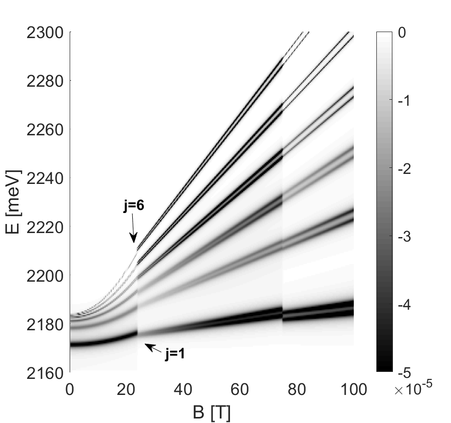
Figure 1: Imaginary part of susceptibility (black color) of a quantum well in Faraday configuration, calculated in three field regimes. The lower limits of intermediate and high field regime are 28 T and 75 T accordingly

The boundaries between low, intermediate and high field regimes are estimated at 28 T and 75 T, which is a close match to the initial estimation of 26.8/29.2 and 74.49/81.36 T for $m\pm 1$, $n=1$ respectively. For such values, there is a very good correspondence between solutions (Eqs. (III.1), (III.3), (III.2) respectively). The lines appear in pairs, corresponding to m=$\pm 1$ and exhibit roughly quadratic energy shift with increasing $B$ in a weak field limit. Such tendency has been also observed in a bulk samples in the experiments and theoretically Rommel ,Zielinska.PRB.2016.c . Due to the fact that the energy shift of all lines is almost linear for B>10 T, the fit is not sensitive to the changes of low, medium and high field boundaries, so that even rough estimations presented above are sufficient to obtain continuous spectrum.

The Fig. 2 depicts the low field solution calculated for a bigger range of quantum numbers $[N,j,m]$, which are given in brackets. It is worth underscore that for QW with REs in a magnetic field these indexes describe three types of of states and three origins of resonances; $N$ arises from confinement in z-direction, number $j$ enumerating excitons is connected with e-h Coulomb interaction and $m$ refers to an interaction with magnetic field resulting with Zeeman splitting with lines shift towards higher energy with increasing field strength.One can observe several interesting tendencies. By increasing $N$, one introduces almost constant energy shift (series of blue lines for $j=2$, orange lines for $j=3$). On the other hand, the lines coming from higher excitonic states (red series) exhibit stronger energy shift with increasing $B$ due to bigger sensitivity of higher states to an external field and finally, the split with respect to $m=\pm 1$ is weaker for the higher $j$ lines. One has to do with an intricate situation of an interplay between Coulomb and magnetic interaction.

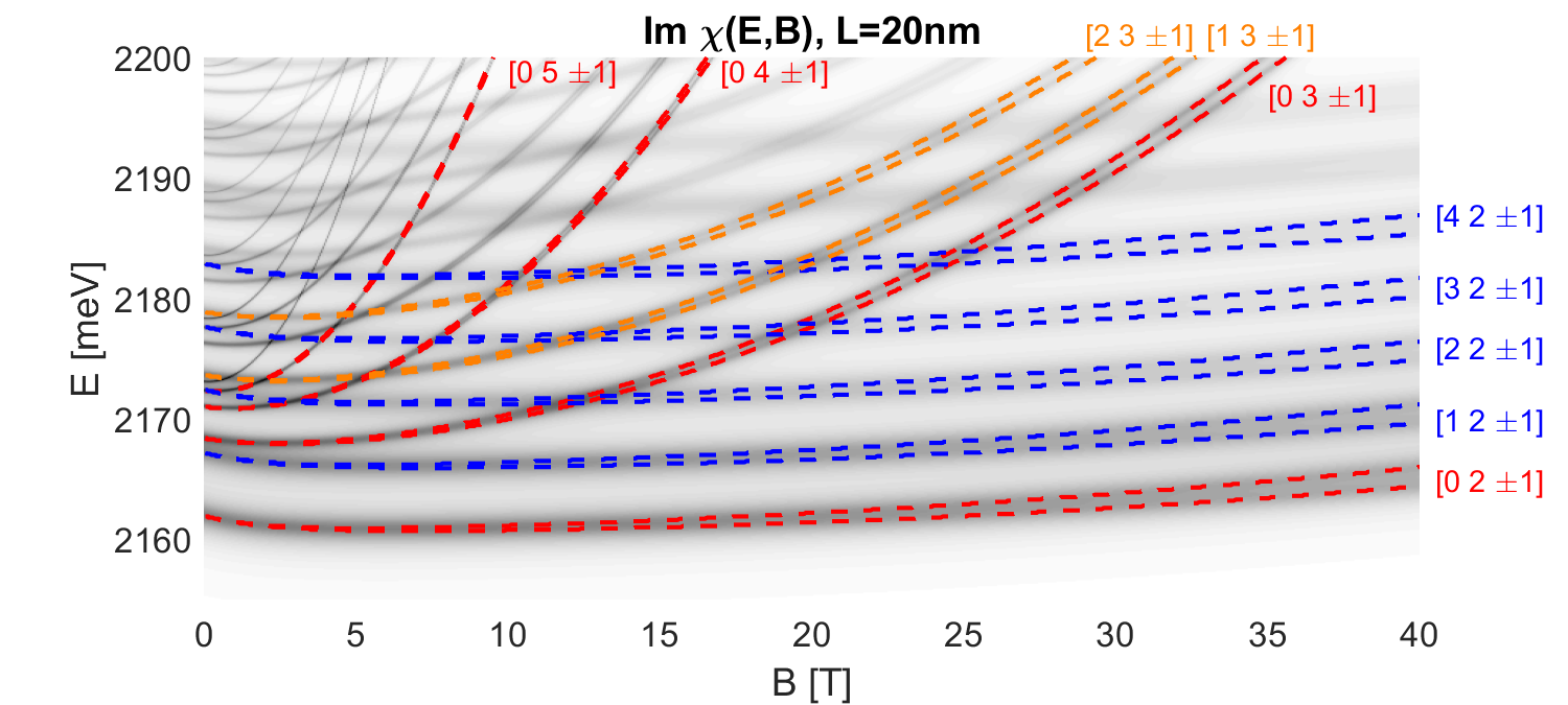
Figure 2: The same as in Fig. 1, calculated for L=20 nm. The brackets denote quantum numbers $[N,j,m]$.

On the Fig. 3 one can observe the dependence of energy shift on the well thickness $L$. As one has expected the confinement effect is more pronounced for narrower QWs. The states with various $N$ (blue lines) split from the respective $j$ state and diverge as $L\rightarrow 0$, with the higher $N$ states approaching $E\rightarrow\infty$ faster due to their lower binding energy and larger physical size, which makes them more affected by finite well size. Higher $N$ states have are more affected by the potential barrier at the quantum well edges. One can observe that the lines with different $j$ (red series) react to the confinement in the same manner - the distance between them remains almost constant up to $L\sim 5$ nm, where the well thickness becomes comparable to the exciton size. The large distance between $j=2$ and $j=3$ states is a result of high magnetic field ($B=50$ T); as mentioned before, lines with different $j$ exhibit different energy shift depending on $B$, which results in increasing distance between them.

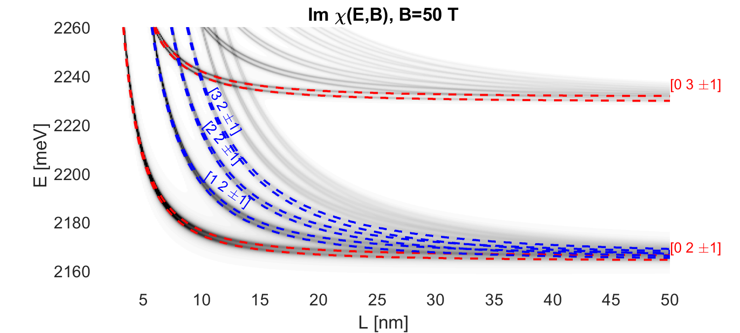
Figure 3: The same as in Fig. 1, calculated for B=20 T. The brackets denote quantum numbers $[N,j,m]$.

The absorption spectrum in Voigt configuration appears to have a more complicated structure. The Fig. 4 shows absorption coefficient calculated from Eq. (III.1) with Eq. (42) for the weak regime Eq. (IV.3) for intermediate regime and from Eq. (IV.2) for the strong regime. The boundaries between regimes are set to 55 T and 140 T. The lower field limit is equal to the initial estimation and the high field limit is somewhat lower than initial estimation (180 T), but its exact location is very flexible due to the fact that energy shifts in both intermediate and strong field solutions are linear. Again, the fit between two regimes is the best for higher energy states. The most striking feature of the spectrum is the grouping of lines corresponding to the same value of $m$ which has the largest contribution to the state energy, especially in the high field regime. The energy shift depending on other quantum numbers ($N$ and $j$) is less pronounced, so that there are groups of lines centered around specific value of $m$.

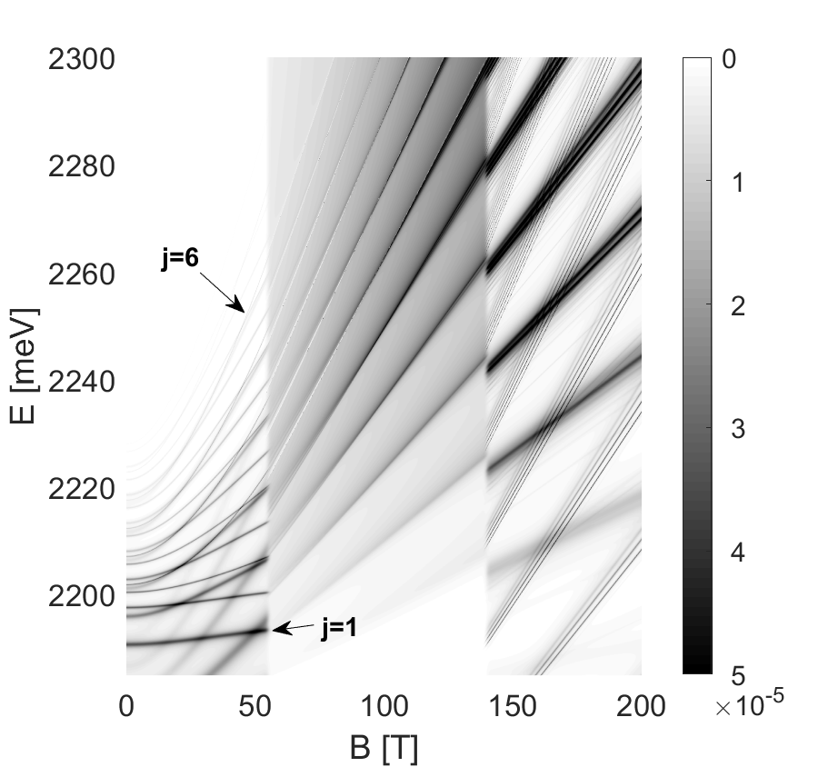
Figure 4: Imaginary part of susceptibility of a quantum well in Voigt configuration calculated for a range of magnetic field strength and $L$=20 nm.

To better discern these states, one can assign the quantum numbers $[N,j,m]$ to them, as shown on the Fig. 5.

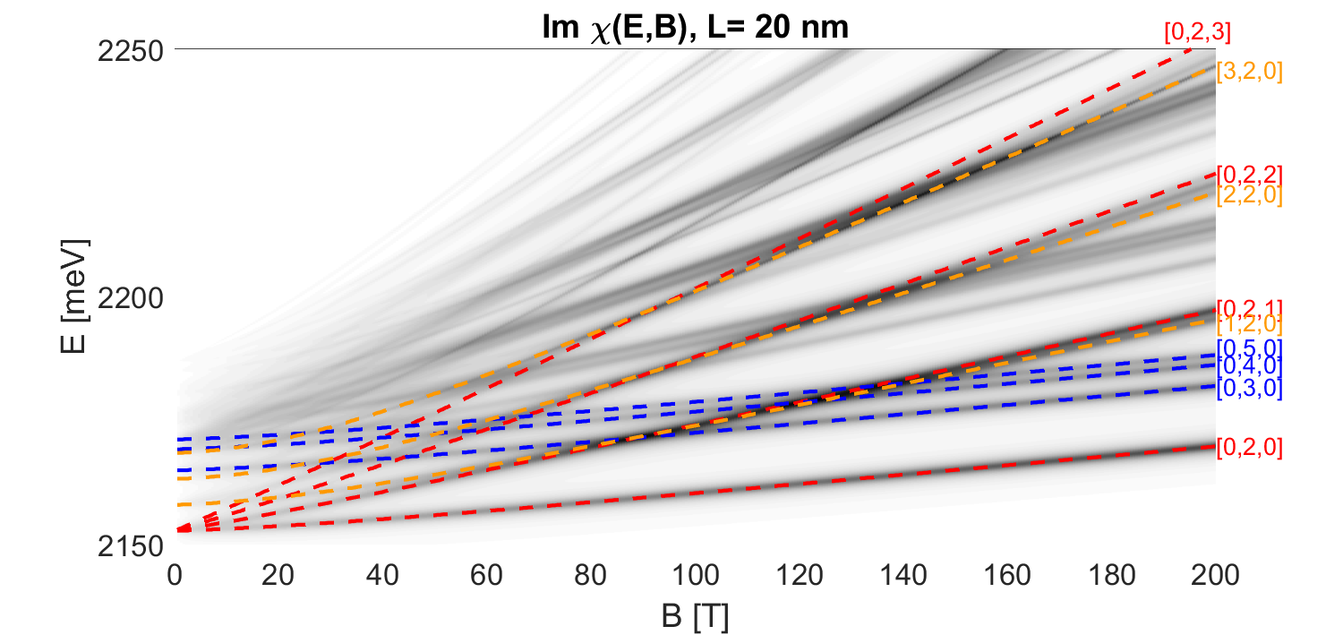
Figure 5: The same as Fig. 4, with states identified by their quantum numbers [N,j,m].

The base state, marked by red line, is $[0,2,0]$ and the other states are created by changing one quantum number. The increase of $j$ (blue lines) yields a typical, excitonic $\sim 1/n^{2}$ energy shift, approaching $E=E_{g}$ at $B=0$. In our model, the distance between excitonic states is independent of $B$. On the other hand, the energy shift with B depends strongly on $N$ and $m$. Every confinement state $N$ undergoes Zeeman split; one can see that the energy of $N=0$ states with various $m$ (red lines) changes linearly with B and these lines start from a common origin at $B=0$. The energy shift for higher $N$ (orange lines) is quadratic in the low field regime, and then transitions to linear at $B\sim 50$ T.

The dependence on the well thickness, shown on the Fig. 6, is also interesting. One can see that similar to the Faraday configuration, the energies diverge at the very low $L$ limit, with the exact location of the asymptote dependent on the quantum numbers $N$ and $j$ due to the fact that the physical size of exciton of any given $j$ affects the energy and the magnetic moment of a bound state depends on quantum number $N$.

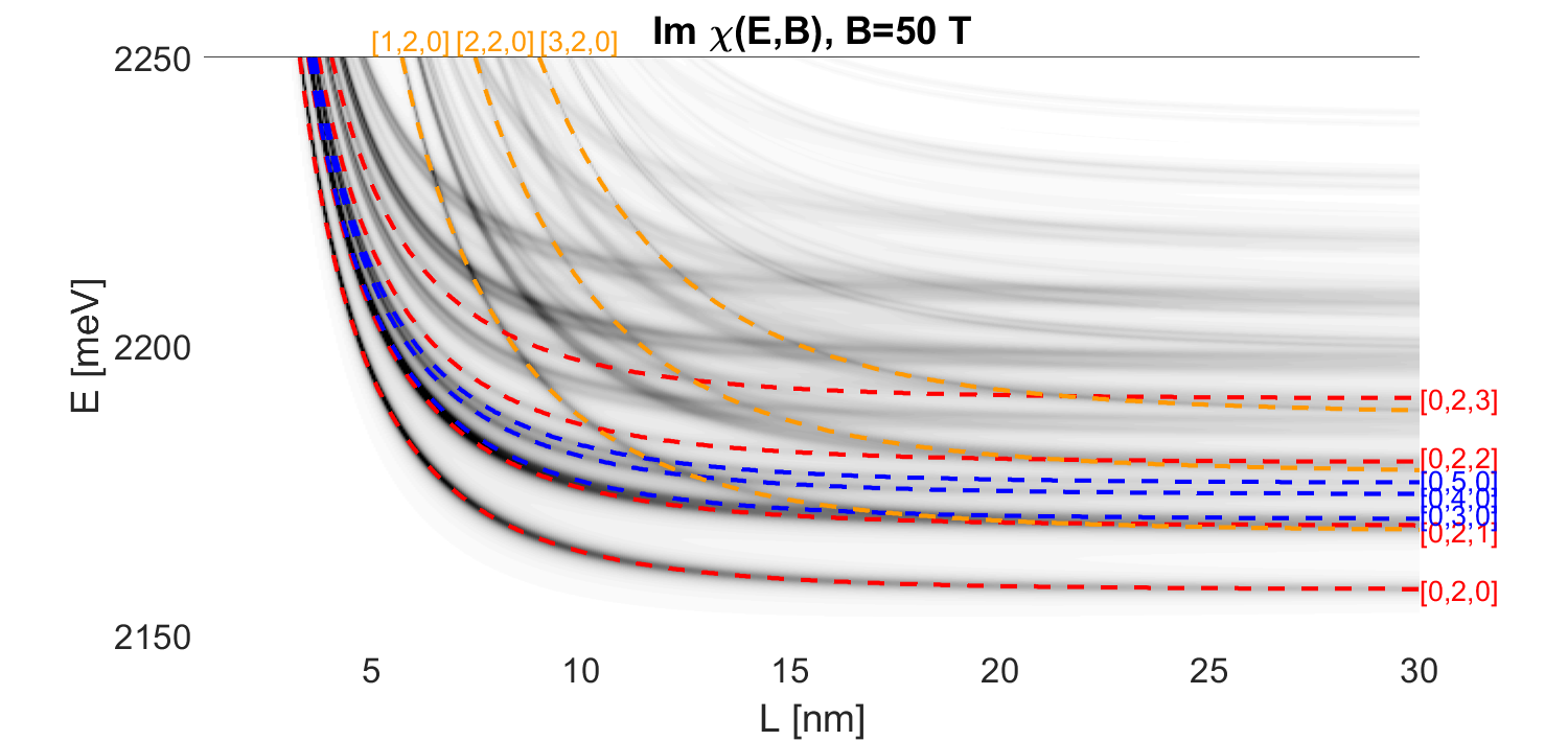
Figure 6: The same as Fig. 4, calculated for $B=50T$ and a range of $L$ values, with states identified by their quantum numbers [N,j,m].

We also have performed the comparison of our theoretical results with available experimental data to verify the accuracy and applicability of our theoretical approach and estimations.

The Fig. 7 shows a comparison between the energy of first confinement state measured in GaAlAs quantum dot in the Faraday configuration Wang and our calculation results for Cu₂O quantum well, obtained for $S$ exciton with $m=0$. For effective evaluation of two very different systems, we use the dimensionless parameter $\gamma$ with appropriate Rydberg energy (87.78 meV for Cu₂O and 8.1 meV for GaAlAsWang ). Furthermore, the significant difference in energy necessitates two y axes to overlap the data. This way, one can observe several similarities. In both systems, the magnetic field induced shift is quadratic in the low field regime and transitions to linear at $\gamma\sim 0.08$, which is consistent with our estimations. It should be stressed out that the results are accurate up to a constant; apart from the difference of band gaps and Rydberg energies, the data for GaAlAs is measured for quantum dots and our calculations have cylindrical symmetry. However, as pointed out in Wang ^, Ziemkiewicz_PRB_2020 , proper adjustment of quantum well size allows for an approximation of a quantum dot, which is sufficient for the sake of presented comparison.

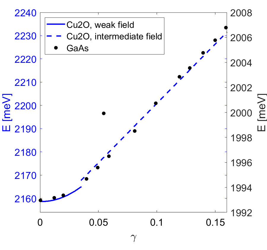
Figure 7: Comparison of the calculated line shape and experimental results by Wang et al Wang for GaAlAs.

The results for the Voigt configuration are compared with InAlAs on the Fig. 8. Again, the estimated boundary between weak and strong field regimes provides a good match to the experimental data.

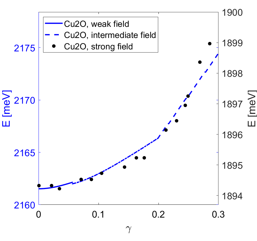
Figure 8: Comparison of the calculated line shape and experimental results by Wang et al Wang for InAlAs.

Finally, we use the experimental results of Jeon et al Jeon to study the effect of well thickness on the energy, marked by $\Delta E=E(B)-E(0)$. One can observe an increase of the confinement energy with thickness $L$. For any fixed value of $B$, reduction of $L$ increases the energy (See Fig. 6); however, confinement states in larger quantum well exhibit stronger reaction to magnetic field, which results in higher energy overall.

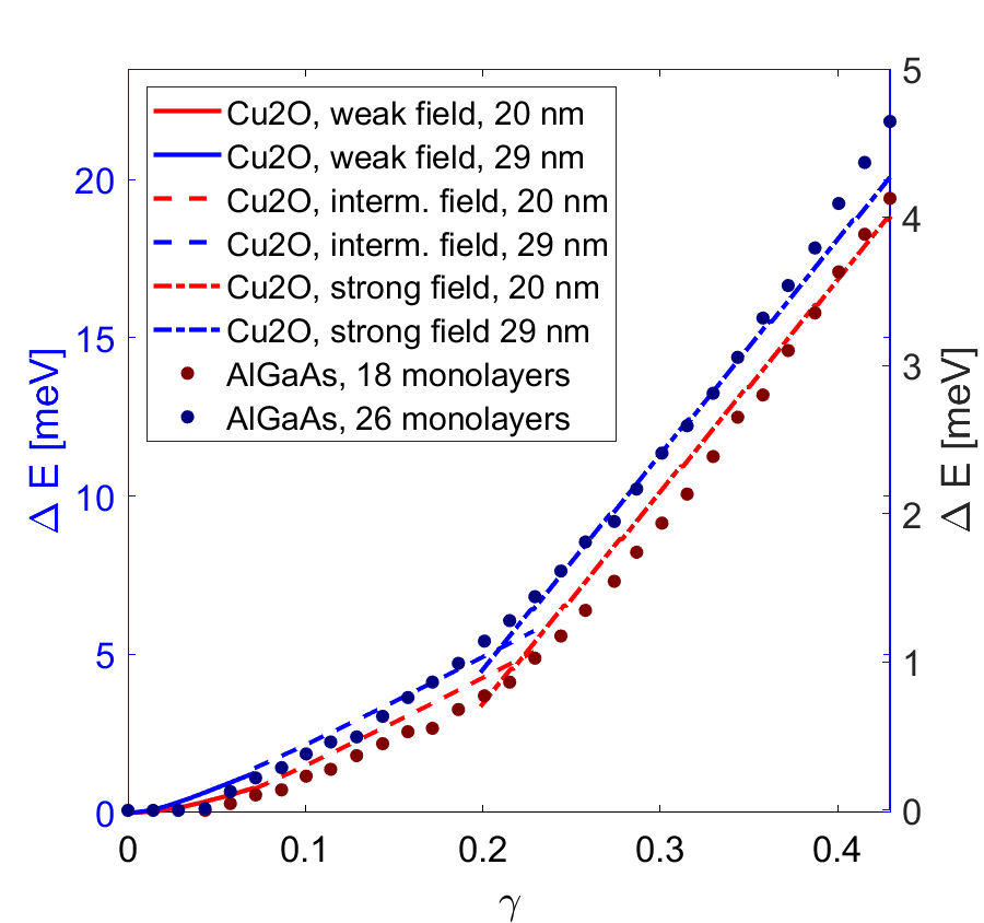
Figure 9: Comparison of the calculated line shape and experimental results by Jeon et al Jeon for GaAs/AlGaAs quantum well.

VI Conclusions

In the present work we have studied the magneto-optical functions for Cu₂O quantum wells with Rydberg excitons at two different orientations of the magnetic field. A theoretical solutions to model absorption spectra due to excitons of Cu₂O in a quantum well in a wide range of magnetic fields is presented, with separate treatment of low, medium and high field regime. The theoretical analysis is done for both Faraday and Voigt external field configuration, including Landau splitting. We observe considerable inter-level mixing and splitting caused by differences in energy shifts of various excitonic states caused by confinement and magnetic field. Key characteristics of Cu₂O excitons - unusually high Rydberg energy, exceptionally large size of higher states and unique ratio of electron to hole mass all play a crucial role in forming rich magnetic absorption spectra. We conclude that in QW the difference between spectra obtained in both configurations depends on degrees of freedom involved in the interaction between the excitons and the magnetic field. Because of that and an effective electron and hole masses ratio we observe that the boundaries of intermediate and strong field regime are significantly higher for the Voigt configuration.

Finally, we introduce a field-dependent parameter $\gamma$ which is a versatile tool for qualitative separation of the magnetic field regimes. Due to its universal nature, it can be employed to compare the calculation results with experimental spectra measured in other semiconductors, serving as a benchmark of the paper.

Appendix A Matrix elements

We calculate the matrix elements (22) using the eigenfunctions (III.1). First we calculate the diagonal elements

$$\;V_{jj}=\frac{\gamma^{2}}{4}\langle R_{j1}(\rho)|\rho^{2}|R_{j1}(\rho)\rangle$$ (61)

$$=\frac{\gamma^{2}}{4}16\lambda^{3}\left[\frac{j!}{(j+2|m|)!}\right]\int\limits_{0}^{\infty}\rho\,d\rho e^{-4\lambda\rho}(4\lambda\rho)^{2}\rho^{2}\left[L_{j}^{2}(4\lambda\rho)\right]^{2}$$

$$=\frac{\gamma^{2}}{64\lambda(j+1)(j+2)}\int\limits_{0}^{\infty}dx\,e^{-x}x^{4}\left[xL^{2}_{j}(x)\right]L^{2}_{j}(x).$$

The integral in the above equation is knownGrad , and we obtained the expression

$$V_{jj1}=\frac{\gamma^{2}(j+2)!}{64\lambda(j+1)(j+2)}4!$$ (62)

$$\times\left\{(2j+3)(j+2)!\left[\frac{1}{j!2!}\right]^{2}+\frac{(j+3)!}{[j!]^{2}\,3!}+\frac{(j+1)(j+2)}{(j-1)!3!}\right\}.$$

The off-diagonal elements can be obtained using Rodrigues^, formula

$$L_{j}^{\alpha}(x)=\sum\limits_{\ell=0}^{j}(-1)^{\ell}{j+\alpha\choose j-\ell}\frac{x^{\ell}}{\ell!}.$$ (63)

Performing the integration we obtain the matrix elements in the form

$$V_{ij1}=\frac{\gamma^{2}}{4}\int\limits_{0}^{\infty}\rho\,d\rho R_{i1}(\rho)\,\rho^{2}\,R_{j1}(\rho)$$

$$=4^{3}\gamma^{2}(\lambda_{i}\lambda_{j})^{5/2}\left[\left(\frac{i!}{(i+2)!}\right)\left(\frac{j!}{(j+2)!}\right)\right]^{1/2}$$ (64)

$$\times\sum\limits_{r=0}^{i}\sum\limits_{s=0}^{j}\Biggl{\{}{i+2\choose i-r}{j+2\choose j-s}\frac{(-1)^{r+s}}{r!s!}$$

$$\times(4\lambda_{i})^{r}(4\lambda_{j})^{s}\frac{(5+r+s)!}{[2(\lambda_{i}+\lambda_{j})]^{5+r+s+1}}\Biggr{\}}.$$

Using the above formula (63) we calculated the matrix elements $V_{n\ell m}$ for the high field limit (III.2). After simple transformations, for the case $|m|=1$, they can be put into the form

$$V_{jk1}=-\frac{2\sqrt{2\gamma}}{\sqrt{(j+1)(k+1)}}\int\limits_{0}^{\infty}dx\,e^{-x^{2}}x^{2}\,L^{1}_{j}(x^{2})L_{k}^{1}(x^{2}),$$

from which one obtains the formula

$$V_{jk1}=-\frac{1}{\sqrt{(j+1)(k+1)}}\sqrt{\frac{\pi\gamma}{2}}$$ (65)

$$\times\sum\limits_{r=0}^{j}\sum\limits_{s=0}^{k}{j+1\choose j-r}{k+1\choose k-s}\frac{(-1)^{r+s}}{r!s!}\frac{(2r+2s+1)!!}{2^{r+s}}.$$

Appendix B Intermediate fields, Faraday configuration

Substituting the trial function (III.3) into the Eq. (30), with $V=-2/\rho$, one obtains the following integral equation

$$\Psi_{00}R_{01}(\rho)\left[\sum\limits_{m=\pm 1}Y_{0m,00}\exp(-\kappa_{0m00}\rho)\frac{e^{im\phi}}{\sqrt{2\pi}}\right]$$

$$+\sum\limits_{n=1}^{\infty}\sum\limits_{N_{e}N_{h}\geq 1}\sum\limits_{m}\frac{e^{im\phi}}{\sqrt{2\pi}}Y_{nmN_{e}N_{h}}R_{nm}(\rho)\Psi_{N_{e}N_{h}}$$ (66)

$$=\frac{2\mu}{\hbar^{2}a^{*}}\left[(M_{0}\rho_{0})\frac{2\gamma}{\sqrt{\pi}}\right]\frac{e^{i\phi}}{\sqrt{2\pi}}\sum\limits_{n=0}^{\infty}R_{n1}(\rho)\frac{d_{n1}}{\kappa^{2}_{n1;N_{e}N_{h}}}$$

$$+\frac{2\mu}{\hbar^{2}a^{*}}\left[(M_{0}\rho_{0})\frac{2\gamma}{\sqrt{\pi}}\right]\frac{e^{-i\phi}}{\sqrt{2\pi}}\sum\limits_{n=0}^{\infty}R_{n1}(\rho)\frac{d_{n1}}{\kappa^{2}_{n,-1;N_{e}N_{h}}}$$

$$+\int\limits_{0}^{\infty}\rho^{\prime}d\rho^{\prime}\int\limits_{0}^{2\pi}d\phi^{\prime}\int\limits_{-\infty}^{\infty}dz_{e}^{\prime}\int\limits_{-\infty}^{\infty}dz_{h}^{\prime}\Biggl{\{}G(\rho,\rho^{\prime};\phi,\phi^{\prime};z_{e},z_{e}^{\prime};z_{h},z_{h}^{\prime})$$

$$\times\frac{2}{\rho^{\prime}}R_{01}(\rho^{\prime})\Psi_{00}(z_{e}^{\prime},z_{h}^{\prime})$$

$$\times\left[\sum\limits_{m=\pm 1}Y_{0m;00}\frac{\exp(-\kappa_{0m;00}\rho^{\prime})}{\kappa^{2}_{nm;N_{e}N_{h}}}\frac{e^{im\phi^{\prime}}}{\sqrt{2\pi}}\right]\Biggr{\}}.$$

From various methods of solving integral equations we choose the method of projection on an orthonormal basis $u_{nm}(\rho,\phi),\Psi_{N_{e}N_{h}}(z_{e},z_{h})$. We can use the functions $\psi_{nm}(\rho)\exp(im\phi)/\sqrt{2\pi}$, to obtain

$$Y_{0m,00}\langle R_{01}^{2}|e^{-\kappa_{0m;00}\rho}=\frac{2\mu}{\hbar^{2}a^{*}}\left[(M_{0}\rho_{0})\frac{2\gamma}{\sqrt{\pi}}\right]{\mathcal{E}}\frac{d_{01}}{\kappa^{2}_{0m;00}}$$

$$+2\sum\limits_{m=\pm 1}Y_{0m,00}\int\limits_{0}^{\infty}d\rho^{\prime}\frac{e^{-\kappa_{0m;00}\rho^{\prime}}}{\kappa^{2}_{0m;00}}R_{01}^{2}(\rho^{\prime}).$$ (67)

From the above equation the parameters $Y_{0m,00}$ and $Y_{nm,00}$ (III.3),(35) were obtained.

Appendix C The coefficients for the adiabatic potentials

The coefficients $a_{2n+1}$ are defined from the relations

$$\langle\psi^{(1D)}_{\beta,N_{y}}(y)|\frac{2}{\sqrt{x^{2}+y^{2}}}|\psi^{(1D)}_{\beta,N_{y}}(y)\rangle=\frac{2}{|x|+a_{N_{y}}},$$

$$\frac{1}{a_{N_{y}}}=\left.\langle\psi^{(1D)}_{\beta,N_{y}}(y)|\frac{2}{\sqrt{x^{2}+y^{2}}}|\psi^{(1D)}_{\beta,N_{y}}(y)\rangle\right|_{x=0}.$$

For odd parity eigenfunctions $N_{y}=2n+1$, and we use the relation between Hermite polynomials and the confluent hypergeometric function

$$\psi^{(1D)}_{2n+1,\beta}(y)=A_{2n+1}H_{2n+1}(\beta y)e^{-\beta^{2}y^{2}/2}$$ (68)

$$=A_{2n+1}(-1)^{n}\,2\frac{(2n+1)!}{n!}\beta y\,M\left(-n,\frac{3}{2},\beta^{2}y^{2}\right)e^{-\beta^{2}y^{2}/2}$$

with the normalization factor $A_{2n+1}.$ The coefficients $a_{2n+1}$ are obtained from the following calculations

$$\frac{1}{a_{2n+1}}=2\int\limits_{0}^{\infty}\left[\psi^{(1D)}_{2n+1,\beta}\right]^{2}\frac{1}{y}dy$$

$$=2\,[A_{2n+1}]^{2}\int\limits_{0}^{\infty}\left[\frac{(2n+1)!}{n!}\right]^{2}4\left[M\left(-n,\frac{3}{2},\beta^{2}y^{2}\right)\right]^{2}$$

$$\times e^{-\beta^{2}y^{2}}\beta^{2}y\,dy$$ (69)

$$=\pi^{-1/2}\frac{\beta\,(2n+1)!}{2^{2n+1}(n!)^{2}}4\int\limits_{0}^{\infty}e^{-z}\left[M\left(-n,\frac{3}{2},z\right)\right]^{2}\,dz$$

$$=\pi^{-1/2}\frac{\beta\,(2n+1)!}{2^{2n-1}(n!)^{2}}J^{n}_{1}.$$

We use the integralLandau

$$J^{n}_{\nu}=\int\limits_{0}^{\infty}e^{-kz}z^{\nu-1}[M(-n,\gamma,kz)]^{2}dz,$$

$$n=0,$$

$$J_{\nu}^{0}=\frac{1}{k^{\nu}}\Gamma(\nu),$$

$$n=1,2,\ldots,$$

$$J^{n}_{\nu}=\frac{\Gamma(\nu)n!}{k^{\nu}\gamma(\gamma+1)\ldots(\gamma+n-1)}\left\{1+\frac{n(\gamma-\nu-1)(\gamma-\nu)}{1^{2}\cdot\gamma}\right.$$

$$\left.+\frac{n(n-1)(\gamma-\nu-2)(\gamma-\nu-1)(\gamma-\nu)(\gamma-\nu+1)}{1^{2}\cdot 2^{2}\cdot\gamma(\gamma+1)}+\ldots+\right.$$

$$\left.+\frac{n(n-1)\ldots 1(\gamma-\nu-n)\ldots(\gamma-\nu+n-1)}{1^{2}\ldots n^{2}\cdot\gamma(\gamma+1)\ldots(\gamma+n-1)}\right\}.$$

In our case we put $k=1,\quad\nu=1,\quad\gamma=\frac{3}{2}$. For the lowest values of $n$ one obtains

$$n=0,\quad J_{1}^{0}=1,\quad\frac{1}{a_{1}}=\pi^{-1/2}\cdot 2\beta,\quad a_{1}=\frac{1}{2}\sqrt{\pi}\beta^{-1},$$

$$n=1,\qquad J_{1}^{1}=\frac{5}{9},\qquad\frac{1}{a_{3}}=\pi^{-1/2}\cdot\frac{5\beta}{3},\quad a_{3}=\frac{3}{5}\sqrt{\pi}\beta^{-1},$$

$$n=2,\quad J_{1}^{2}=\frac{2}{5},\quad\frac{1}{a_{5}}=\pi^{-1/2}\cdot\frac{3}{2}\beta,\quad a_{5}=\frac{2}{3}\sqrt{\pi}\beta^{-1}.$$

Appendix D Determination of parameters, Voigt configuration, intermediate fields

Inserting the trial function (57) into Eq. (31), and using the Green function (IV.3), one obtains the equation and retaining the lowest expansion term in $GVY$ one obtains the following expression

$$Y_{0}\Psi_{00}(z_{e},z_{h})\psi_{1,\beta}^{(1D)}(y)e^{-\kappa_{0}\sqrt{x^{2}+y^{2}}}$$

$$+\sum\limits_{n=1}^{\infty}\sum\limits_{N_{e}N_{h}\geq 1}\psi_{2n+1,\beta}^{(1D)}(y)\Psi_{N_{e}N_{h}}(z_{e},z_{h})\frac{1}{2\pi}\int\limits_{-\infty}^{\infty}dk\,Y_{nN_{e}N_{h}}(k)e^{ikx}$$

$$=\frac{2\mu}{\hbar^{2}a^{*}}{\mathcal{E}}\frac{(M_{0}\rho_{0})}{\sqrt{2\pi}}\sum\limits_{n}\sum\limits_{N_{e}}\sum\limits_{N_{h}}g_{2n+1}\psi_{2n+1,\beta}^{(1D)}(y)$$

$$\times\Psi_{N_{e}N_{h}}(z_{e},z_{h})\delta_{N_{e}N_{h}}\int\limits_{-\infty}^{\infty}\frac{dke^{ikx}\,e^{-k^{2}\rho_{0}^{2}/2}}{k^{2}+\kappa_{nN_{e}N_{h}}^{2}}$$

$$+4Y_{0}\sum\limits_{n,N_{e},N_{h}}\int\limits_{-\infty}^{\infty}dz_{e}^{\prime}\int\limits_{-\infty}^{\infty}dz_{h}^{\prime}$$

$$\times\frac{1}{2\pi}\int\limits_{0}^{\infty}dx^{\prime}\int\limits_{-\infty}^{\infty}dy^{\prime}\int\limits_{-\infty}^{\infty}dk\,e^{ikx}\cos kx^{\prime}\,\psi^{(1D)}_{\beta,n}(y)\psi^{(1D)}_{\beta,n}(y^{\prime})$$

$$\times\frac{\psi^{(1D)}_{\alpha_{e}^{V},N_{e}}(z_{e})\psi^{(1D)}_{\alpha_{e}^{V},N_{e}}(z_{e}^{\prime})\psi^{(1D)}_{\alpha_{h}^{V},N_{h}}(z_{h})\psi^{(1D)}_{\alpha_{h}^{V},N_{h}}(z^{\prime}_{h})}{k^{2}+\kappa_{nN_{e}N_{h}}^{2}}$$

$$\times\frac{\exp(-\kappa_{0}\sqrt{x^{\prime 2}+y^{\prime 2}})}{\sqrt{x^{\prime 2}+y^{\prime 2}}}\psi^{(1D)}_{\beta,1}(y^{\prime})\Psi_{00}(z_{e}^{\prime}z_{h}^{\prime})$$

Similar equation has been obtained in Appendix B, and was solved by making projections on a orthonormal set of functions. Here we choose the functions $\{\psi^{(1D)}_{\beta,n}(y)\},\Psi_{N_{e}N_{h}}$, put $x=0$, and obtain

$$Y_{0}=\frac{2\mu}{\hbar^{2}a^{*}}{\mathcal{E}}\frac{(M_{0}\rho_{0})}{\sqrt{\pi}}\frac{{g_{1}}}{\kappa_{0}}$$

$$\times\left[\frac{2^{3/2}}{\sqrt{\pi}}e^{\kappa_{0}^{2}/8\beta^{2}}D_{-3}\left(\frac{\kappa_{0}}{\beta\sqrt{2}}\right)-F(\kappa_{0},\beta)\right]^{-1},$$ (70)

$$F(\kappa_{0},\beta)=\frac{\beta}{\sqrt{\pi}}\int\limits_{-\infty}^{\infty}\,dk\,\frac{e^{-k^{2}\rho_{0}^{2}/2}}{(k^{2}+\kappa_{0}^{2})^{3/2}}$$

$$\times\exp\left(\frac{k^{2}+\kappa_{0}^{2}}{8\beta^{2}}\right)W_{-1,0}\left(\frac{k^{2}+\kappa_{0}^{2}}{4\beta^{2}}\right),$$

$$\frac{1}{2\pi}Y_{nN}(k)=\frac{2\mu}{\hbar^{2}a^{*}}{\mathcal{E}}\frac{M_{0}\rho_{0}}{\sqrt{2\pi}}g_{2n+1}\,\frac{e^{-k^{2}\rho_{0}^{2}}}{k^{2}+\kappa_{nN}^{2}}.$$

The above quantities, substituted in Eq. (57), determine the exciton amplitude $Y$, which inserted in Eq. (20), gives the magneto-susceptibility (IV.3).

References

• (1) T. Kazimierczuk, D. Fröhlich, S. Scheel, H. Stolz, and M. Bayer, Nature 514, 344 (2014).
• (2) M. Aßmann and M. Bayer, Semiconductor Rydberg Physics, Advanced Quantum technologies, 1900134 (2020). DOI: 10.1002/qute.201900134.
• (3) P. Rommel, F. Schweiner, J. Main, J. Heckötter, M. Freitag, M. Freitag, D. Fröhlich, M. Aßmann, M. Bayer, Phys. Rev. B 98, 085206 (2018).
• (4) J. Thewes, J. Heckötter, T. Kazimierczuk, M. Aßmann, D. Fröhlich, M. Bayer, M. A. Semina, and M. M. Glazov, Phys. Rev. Lett. 115, 027402 (2015).
• (5) F. Schöne, S.-O. Krüger, P.Grünwald, H. Stolz, M. Aßmann, J. Heckötter, J. Thewes, D. Fröhlich, and M. Bayer, Phys. Rev. B 93, 075203 (2016).
• (6) F. Schweiner, J. Main, and G. Wunner, Phys. Rev. B 95, 035202 (2017).
• (7) S. Zielinska-Raczyńska, D. A. Fishman, C. Faugeras, M. M. P. Potemski, P. H. M. van Loosdrecht, K. Karpiński, G. Czajkowski, and D. Ziemkiewicz, New J. Phys. 21, 103012 (2019).
• (8) S. Zielińska-Raczyńska, D. Ziemkiewicz, and G. Czajkowski, Phys. Rev. B 95, 075204 (2017).
• (9) D. Ziemkiewicz, K. Karpiński, G. Czajkowski, and S. Zielińska-Raczyńska, Phys. Rev. B 101, 205202 (2020).
• (10) N. Naka, I. Akimoto, M. Shirai, and Ken-ichi Kan’no, Phys. Rev. B 85, 035209 (2012).
• (11) M. Takahata, K. Tanaka, and N. Naka, Phys. Rev. B 97, 205305 (2018).
• (12) A. Konzelmann, B. Frank, and H. Giessen, Phys. B: At. Mol. Opt. Phys. 53, 024001 (2020).
• (13) S. Zielińska-Raczyńska, D. Ziemkiewicz, and G. Czajkowski, Phys. Rev. B 93, 075206 (2016).
• (14) A. Stahl, I. Balslev, Electrodynamics of the semiconductor band edge, Springer, 1987.
• (15) J. Heckötter, D. Frölich, M. Aßmann, and M. Bayer, Physics of the Solid State 60, 1595 (2018).
• (16) S. Zielińska-Raczyńska, G. Czajkowski, and D. Ziemkiewicz, Phys. Rev. B 93, 075206 (2016).
• (17) S. Zielińska-Raczyńska, D. Ziemkiewicz, and G. Czajkowski, Phys. Rev. B 94, 045205 (2016).
• (18) M. Abramowitz and I. Stegun, Handbook of Mathematical Functions (Dover Publications, New York, 1965).
• (19) I. S. Gradshteyn and I. M. Ryzhik, Table of Integrals, Series, and Products, edited by A. Jeffrey and D. Zwillinger, 7th Edition (Academic Press, Elsevier, Amsterdam, 2007, ISBN-13:978-0-12-373637-6).
• (20) N. F. Mott and H. S. W. Masey, The theory of atomic collisions (Clarendon Press, Oxford, 1965).
• (21) H. Stolz, F. Schöne, and D. Semkat, N. Journ. Phys. 20, 023019 (2018).
• (22) D. Ziemkiewicz, S. Zielińska - Raczyńska, Optics Express 27, 16983 (2019).
• (23) G. Czajkowski, F. Bassani, and L. Silvestri, Rivista del Nuovo Cimento 26, 1-150 (2003).
• (24) P. D. Wang, J. L. Merz, S. Fafard, R. Leon, D. Leonard, G. Medeiros-Ribeiro, M. Oestreich, and P. M. Petroff, K. Uchida and N. Miura, Phys. Rev. B 53, 16 458 (1996).
• (25) A. V. Chernenko, P. S. Dorozhkin, V. D. Kulakovskii, A. S. Brichkin ,Ivanov and A. A. Toropov, Phys. Rev. B. 72, 045302 (2005).
• (26) M.H. Jeon, K.H. Yooa, M.G. Sung, I. T. Jeong, J.C. Woo, L.R. Ram-Mohan, Solid State Communications 150, 1782–1784 (2010).
• (27) L. D. Landau and E. M. Lifshitz, Quantum Mechanics (Pergamon Press, Oxford, 1963).