Exploding operators for Majorana neutrino masses and beyond

Abstract

Building UV completions of lepton-number-violating effective operators has proved to be a useful way of studying and classifying models of Majorana neutrino mass. In this paper we describe and implement an algorithm that systematises this model-building procedure. We use the algorithm to generate computational representations of all of the tree-level completions of the operators up to and including mass-dimension 11. Almost all of these correspond to models of radiative neutrino mass. Our work includes operators involving derivatives, updated estimates for the bounds on the new-physics scale associated with each operator, an analysis of various features of the models, and a look at some examples. We find that a number of operators do not admit any completions not also generating lower-dimensional operators or larger contributions to the neutrino mass, ruling them out as playing a dominant role in the neutrino-mass generation. Additionally, we show that there are at most five models containing three or fewer exotic multiplets that predict new physics that must lie below 100 TeV. Accompanying this work we also make available a searchable database containing all of our results and the code used to find the completions. We emphasise that our methods extend beyond the study of neutrino-mass models, and may be useful for generating completions of high-dimensional operators in other effective field theories.

Example code:

1 Introduction

Laboratory experiments to date have firmly established the predictive power of the Standard Model (SM). Mass generation for the weak gauge bosons and charged fermions is by now a familiar narrative, and the only clear terrestrial measurements pointing to physics beyond the SM are those of neutrino flavour transformations. Even here, observations are consistent with the prevailing orthodoxy: the neutrino flavour eigenstates are unitary superpositions of mass eigenstates and the probability of detecting a neutrino of a given flavour oscillates with distance. On the origin of these neutrino oscillations — and the non-zero neutrino masses they imply — the SM has nothing to say. Oscillation experiments have shown that the mixing in the lepton sector is of a different structure and extent to that seen in quarks; and measurements from cosmology, neutrinoless double-beta decay and tritium beta decay strongly constrain the absolute scale of the neutrino masses. These facts lend themselves to the possibility that an alternate mass-generating mechanism is operating for the uncharged leptons.

A characteristic feature of the neutrinos is that they are the only fermions in the SM that could acquire a Majorana mass, as long as lepton number isn’t endowed with any special significance. Many models pursue this line of reasoning, with the neutrinos acquiring a Majorana mass through the lepton-number-violating (LNV) interactions of heavy exotica. The most famous examples are the three canonical seesaw models MINKOWSKI1977421 ; Yanagida:1979as ; GellMann:1980vs ; PhysRevLett.44.912 ; Glashow:1979nm ; Magg:1980ut ; PhysRevD.22.2227 ; LAZARIDES1981287 ; Wetterich:1981bx ; PhysRevD.23.165 ; Foot:1988aq that generate the dimension-five Weinberg operator $(L^{i}L^{j})H^{k}H^{l}\epsilon_{ik}\epsilon_{jl}$ at tree-level upon integrating out the heavy fields. Additionally, the historically important Zee Zee:1980ai and Zee–Babu Zee:1985id ; Babu:1988ki models have come to be archetypal radiative scenarios in which interactions violating lepton-number by two units ($\Delta L=2$) generate a Majorana mass for the neutrinos at loop level. Such models are economic, since they do not require the imposition of ad hoc symmetries, and in many cases make a connection to other unsolved problems of the SM such as the nature of dark matter or the matter–antimatter asymmetry of the Universe. They are also elegant, since the smallness of the neutrino masses emerges as a natural consequence, rather than through the imposed requirement of exceedingly small coupling constants. For recent reviews of radiative models see Refs. Boucenna:2014zba ; Cai:2017jrq .

Although the seesaw models are attractive solutions to the neutrino mass problem, they are difficult to test experimentally. The region of their parameter space in which the seesaw field’s couplings to the SM are very small can be probed at colliders Cai:2017mow , although for $\mathcal{O}(1)$ couplings the seesaw scale is predicted to be $\sim 10^{12}~{}\text{TeV}$. Radiative models are easier to probe experimentally since the additional loop suppression and products of couplings bring down the allowed scale of the new physics, in some cases to LHC-accessible energy ranges deGouvea:2007qla . The two-loop Zee–Babu model, for example, is non-trivially constrained by same-sign dilepton searches performed by ATLAS ATLAS:2012hi ; ATLAS:2014kca ; Aaboud:2017qph and CMS Chatrchyan:2012ya ; CMS:2016cpz ; CMS:2017pet , but it is only one of a very large number of radiative models, none of which are a priori more likely to be true than any other. In the context of such a large theory-space, it is useful to have an organising principle to aid in the study and classification of these models, and beginning with $\Delta L=2$ effective operators has been shown to be an effective strategy.

One approach to this model taxonomy involves studying loop-level completions of the Weinberg operator, and its dimension-($5+2n$) generalisations $\mathcal{O}_{1}^{\prime\cdots\prime}=(LL)HH(H^{\dagger}H)^{n}$. Here, models can be systematically written down by studying the various topologies able to be accommodated by the operator with increasing number of loops. This is done in such a way that models implying lower-order contributions to the neutrino mass can be discarded Farzan:2012ev . Such an approach has been applied to the Weinberg operator up to three loops Bonnet:2012kz ; Sierra:2014rxa ; Cepedello:2018rfh and to its dimension-seven generalisation at one loop Cepedello:2017eqf . An alternative and complementary method begins by considering all of the gauge-invariant $\Delta L=2$ operators in the SM effective field theory (SMEFT), first listed in this context by Babu and Leung (BL) Babu:2001ex and extended by de Gouvêa and Jenkins (dGJ) deGouvea:2007qla . Supposing that the tree-level coefficient of one of these is non-zero at the high scale, neutrino masses will be generated from loop graphs contributing to the mixing of this operator and the Weinberg-like operators $\mathcal{O}_{1}^{\prime\cdots\prime}$. The process of expanding the operator into a series of UV-complete, renormalisable models that generate the parent operator at tree-level is called opening up or exploding the operator. The remaining external fields must be looped-off, with additional loops of SM gauge bosons or Higgs fields added as necessary in order to obtain a neutrino self-energy diagram. A model-building formula along these lines has been formulated in Ref. PhysRevD.87.073007 , and it has been used to write down all of the minimal, tree-level UV-completions of $\Delta L=2$ operators at dimension seven Cai:2014kra corresponding to tree-level and radiative neutrino-mass models. The tree-level completions of the Weinberg-like operators have been written down up to dimension eleven Cai:2014kra ; Bonnet:2009ej ; Anamiati:2018cuq .

Our analysis continues in the tradition Refs. Babu:2001ex ; deGouvea:2007qla ; PhysRevD.87.073007 ; Cai:2014kra , but where appropriate we make a connection to the results from loop-level matching Bonnet:2012kz ; Sierra:2014rxa ; Cepedello:2017eqf ; Cepedello:2018rfh for completeness. We consider that there is complementary insight to be gained from thorough and complete analyses involving both approaches. Building models from tree-level completions of the $\Delta L=2$ operators allows for a direct connection to be made between the neutrino-mass mechanism and other lepton-number-violating phenomena. The models derived in this way are also minimal in the sense that they involve the fewest number of exotic fields required to furnish a given loop-level topology, since the neutrino self-energy graphs always involve some SM fields. This has a number of important implications. First, the neutrino masses depend on SM parameters, and their rough scale can therefore be readily estimated from the effective operator alone. Second, neutrino-mass mechanisms containing SM gauge bosons are included automatically, and these constitute a large fraction of the models. Finally, it also means that our approach never produces models that contain loops of only exotic fields, although these can be added easily (see, for example, section IV.C of Ref. PhysRevD.87.073007 ). The appeal of these models notwithstanding, a benefit of giving up heavy loops is that the transformation properties of the beyond-the-standard-model particle content of each model are now uniquely determined, and therefore the total number of minimal models is finite. Minimal exotic particle content, in the aforementioned sense, is an attractive feature of this approach. Indeed, there are many examples of operators whose insertion and closure lead to neutrino masses at dimension nine and higher, but for which the number of exotic degrees of freedom introduced are not more than those of a garden-variety model generating the Weinberg operator at the low scale. The consideration of such equally simple models in the loop-level matching paradigm would require a detailed analysis of the dimension-seven and dimension-nine analogues of the Weinberg operator up to a large number of loops.

An economic classification scheme, separate from an EFT framework, was presented in Ref. Klein:2019iws based on the number of exotic degrees of freedom by which the SM is extended. There, the method is applied to the case of radiative models with two exotics, and has also been used to study minimal neutrino-mass models compatible with $\mathrm{SU}(5)$ unification Klein:2019jgb .

Here, we sharpen the model building prescription developed in Ref. PhysRevD.87.073007 and extend it to the case of operators involving field-strength tensors and derivatives. This procedure is automated and applied to all $\Delta L=2$ operators in the SM effective field theory up to dimension eleven. We classify the neutrino-mass topologies, completions and their exotic fields. We also make available a database containing our main results and example code used to generate the operators along with their completions and Lagrangians neutrinomass2020 . We emphasise that the usefulness of these methods and tools extends beyond the study of neutrino mass and lepton-number-violating phenomena. To illustrate this point we reproduce some recent results of work listing completions of SMEFT operators deBlas:2017xtg .

The remainder of the paper is structured as follows. Section 2.1 sets out our mathematical conventions and notation. Section 3 contains a review of tree-level matching and a description of the methods we use to find the tree-level completions of the operators. Neutrino mass model building is described in section 4, while section 5 presents a preliminary analysis of the models along with some examples.

2 Conventions

In this section we establish the conventions we employ throughout the rest of the paper: the nomenclature of fields and indices, our operational semantics and the classification of the lepton-number-violating operators on which our analysis is based. We highlight that this classification differs mildly from that found in earlier work, since our list includes additional structures as well as operators containing derivatives. We find the operators containing field-strength tensors to be uninteresting from the perspective of model building — a point justified in detail in Sec. 3.2.1 — and choose not to include them in our classification in this section.

2.1 Mathematical notation

Throughout the paper we choose to label representations by their dimension, which we typeset in bold. Multiplets are labelled by their transformation properties under the Lorentz group and the SM gauge group $\mathrm{SU}(3)_{c}\otimes\mathrm{SU}(2)_{L}\otimes\mathrm{U}(1)_{Y}$, and we often refer to them simply as fields. All spinors are treated as two-component objects transforming as either $(\mathbf{2},\mathbf{1})$ (left-handed) or $(\mathbf{1},\mathbf{2})$ (right-handed) under the Lorentz group, written as $\mathrm{SU}(2)_{+}\otimes\mathrm{SU}(2)_{-}$. The left-handed spinors carry undotted spinor indices $\alpha,\beta,\ldots\in\{1,2\}$, while the right-handed spinors carry dotted indices $\dot{\alpha},\dot{\beta},\ldots\in\{\dot{1},\dot{2}\}$. Wherever possible we attempt to conform to the conventions of Ref. Dreiner:2008tw when working with spinor fields (see appendix G for the correspondence to four-component notation and appendix J for SM-fermion nomenclature). For objects carrying a single spacetime index $V_{\mu}$ we define

$$V_{\alpha\dot{\beta}}=\sigma^{\mu}_{\alpha\dot{\beta}}V_{\mu}\quad\text{ and }\quad\bar{V}_{\dot{\alpha}\beta}=\bar{\sigma}^{\mu}_{\dot{\alpha}\beta}V_{\mu}.$$ (1)

Note that in this notation

$$\Box=\partial_{\mu}\partial^{\mu}=\tfrac{1}{2}\text{Tr}[\partial\bar{\partial}]=\tfrac{1}{2}\text{Tr}[\bar{\partial}\partial],$$ (2)

and we will sometimes just use $\Box$ to represent the contraction of two covariant derivatives $D_{\mu}D^{\mu}$ where this is clear from context. For field-strength tensors, generically $X_{\mu\nu}$, we work with the irreducible representations (irreps) $X_{\alpha\beta}$ and $\bar{X}_{\dot{\alpha}\dot{\beta}}$, where

$$X_{\{\alpha\beta\}}=2i[\sigma^{\mu\nu}]^{~{}\gamma}_{\alpha}\epsilon_{\gamma\beta}X_{\mu\nu}\quad\text{ and }\quad\bar{X}_{\{\dot{\alpha}\dot{\beta}\}}=2i[\bar{\sigma}^{\mu\nu}]^{\dot{\gamma}}_{~{}\dot{\beta}}\epsilon_{\dot{\alpha}\dot{\gamma}}X_{\mu\nu},$$ (3)

or the alternate forms with one raised and one lowered index.

Indices for $\mathrm{SU}(2)_{L}$ (isospin) are taken from the middle of the Latin alphabet. These are kept lowercase for the fundamental representation for which $i,j,k,\ldots\in\{1,2\}$ and the indices of the adjoint are capitalised $I,J,K,\ldots\in\{1,2,3\}$. Colour indices are taken from the beginning of the Latin alphabet and the same distinction between lowercase and uppercase letters is made. For both $\mathrm{SU}(2)$ and $\mathrm{SU}(3)$, a distinction between raised and lowered indices is maintained such that, for example, $(\psi^{i})^{\dagger}=(\psi^{\dagger})_{i}$ for an isodoublet field $\psi$. However, we often specialise to the case of only raised, symmetrised indices for $\mathrm{SU}(2)$, and use a tilde to denote a conjugate field whose $\mathrm{SU}(2)_{L}$ indices have been raised:

$$\tilde{\psi}^{i}\equiv\epsilon^{ij}\psi^{\dagger}_{j}.$$ (4)

We adopt this notation from the usual definition of $\tilde{H}$, and note that throughout the paper we freely interchange between $\tilde{\psi}^{i}$ and $\psi^{\dagger}_{i}$. For the sake of tidiness, we sometimes use parentheses $(\cdots)$ to indicate the contraction of suppressed indices. Curly braces are reserved to indicate symmetrised indices $\{\cdots\}$ and square brackets enclose antisymmetrised indices $[\cdots]$, but this notation is avoided when the permutation symmetry between indices is clear. We use $\tau^{I}$ and $\lambda^{A}$ for the Pauli and Gell-Mann matrices, and normalise the non-abelian vector potentials of the SM such that

$$(W_{\alpha\dot{\beta}})^{i}_{\ j}=\frac{1}{2}(\tau^{I})^{i}_{\ j}W^{I}_{\alpha\dot{\beta}}\quad\text{ and }\quad(G_{\alpha\dot{\beta}})^{a}_{\ b}=\frac{1}{2}(\lambda^{A})^{a}_{\ b}G^{A}_{\alpha\dot{\beta}}.$$ (5)

Flavour (or family) indices of the SM fermions are represented by the lowercase Latin letters $\{r,s,t,u,v,w\}$.

For the non-gauge degrees of freedom in the SM we capitalise isospin doublets ($Q$, $L$, $H$), while the left-handed isosinglets are written in lowercase with a bar featuring as a part of the name of the field ($\bar{u}$, $\bar{d}$, $\bar{e}$). The representations and hypercharges for the SM field content are summarised in Table 1. Our definition of the SM gauge-covariant derivative is exemplified by

$$\bar{D}_{\dot{\alpha}\beta}Q^{\beta ai}_{r}=\left[\delta^{a}_{b}\delta^{i}_{j}(\bar{\partial}_{\dot{\alpha}\beta}+ig_{1}Y_{Q}\bar{B}_{\dot{\alpha}\beta})+ig_{2}\delta^{a}_{b}(\bar{W}_{\dot{\alpha}\beta})^{i}_{\ j}+ig_{3}\delta^{i}_{j}(\bar{G}_{\dot{\alpha}\beta})^{a}_{\ b}\right]Q_{r}^{\beta bj}\ .$$ (6)

Note that the derivative implicitly carries $\mathrm{SU}(2)_{L}$ and $\mathrm{SU}(3)_{c}$ indices [explicit on the right-hand side of Eq. (6)] which are suppressed on the left-hand side to reduce clutter. Where appropriate we show these indices explicitly.

Field	$\mathrm{SU}(3)_{c}\otimes\mathrm{SU}(2)_{L}\otimes\mathrm{U}(1)_{Y}$	$\mathrm{SU}(2)_{+}\otimes\mathrm{SU}(2)_{-}$
$Q^{\alpha ai}$	$(\mathbf{3},\mathbf{2},\tfrac{1}{6})$	$(\mathbf{2},\mathbf{1})$
$L^{\alpha i}$	$(\mathbf{1},\mathbf{2},-\tfrac{1}{2})$	$(\mathbf{2},\mathbf{1})$
$\bar{u}^{\alpha}_{a}$	$(\bar{\mathbf{3}},\mathbf{1},-\tfrac{2}{3})$	$(\mathbf{2},\mathbf{1})$
$\bar{d}^{\alpha}_{a}$	$(\bar{\mathbf{3}},\mathbf{1},\tfrac{1}{3})$	$(\mathbf{2},\mathbf{1})$
$\bar{e}^{\alpha}$	$(\mathbf{1},\mathbf{1},1)$	$(\mathbf{2},\mathbf{1})$
$(G_{\alpha\beta})^{a}_{\ b}$	$(\mathbf{8},\mathbf{1},0)$	$(\mathbf{3},\mathbf{1})$
$(W_{\alpha\beta})^{i}_{\ j}$	$(\mathbf{1},\mathbf{3},0)$	$(\mathbf{3},\mathbf{1})$
$B_{\alpha\beta}$	$(\mathbf{1},\mathbf{1},0)$	$(\mathbf{3},\mathbf{1})$
$H^{i}$	$(\mathbf{1},\mathbf{2},\tfrac{1}{2})$	$(\mathbf{1},\mathbf{1})$

Table 1: The SM fields and their transformation properties under the SM gauge group $G_{\text{SM}}$ and the Lorentz group. The final unbolded number in the 3-tuples of the $G_{\text{SM}}$ column represents the $\mathrm{U}(1)_{Y}$ charge of the field, normalised such that $Q=I_{3}+Y$. For the fermions a generational index has been suppressed.

We represent the SM quantum numbers of fields as a 3-tuple $(\mathbf{C},\mathbf{I},Y)_{L}$, with $\mathbf{C}$ and $\mathbf{I}$ the dimension of the colour and isospin representations, $Y$ the hypercharge of the field, and $L$ an (often omitted) label of the Lorentz representation: $S$ (scalar), $F$ (fermion) or $V$ (vector), although sometimes we use the irrep, e.g. $(\mathbf{2},\mathbf{1})$. We normalise the hypercharge such that $Q=I_{3}+Y$. Finally, for exotic fields that contribute to dimension-six operators at tree-level, we try and adopt names consistent with Tables 1 and 2 of Ref. deBlas:2017xtg , which we reproduce here in Table 2.

Name	${\cal S}$	${\cal S}_{1}$	${\cal S}_{2}$	$\varphi$	$\Xi$	$\Xi_{1}$	$\Theta_{1}$	$\Theta_{3}$
Irrep	$(\mathbf{1},\mathbf{1},0)$	$(\mathbf{1},\mathbf{1},1)$	$(\mathbf{1},\mathbf{1},2)$	$(\mathbf{1},\mathbf{2},{\tfrac{1}{2}})$	$(\mathbf{1},\mathbf{3},0)$	$(\mathbf{1},\mathbf{3},1)$	$(\mathbf{1},\mathbf{4},{\tfrac{1}{2}})$	$(\mathbf{1},\mathbf{4},{\tfrac{3}{2}})$
Name	${\omega}_{1}$	${\omega}_{2}$	${\omega}_{4}$	$\Pi_{1}$	$\Pi_{7}$	$\zeta$
Irrep	$(\mathbf{\bar{3}},\mathbf{1},{\tfrac{1}{3}})$	$(\mathbf{3},\mathbf{1},{\tfrac{2}{3}})$	$(\mathbf{\bar{3}},\mathbf{1},{\tfrac{4}{3}})$	$(\mathbf{3},\mathbf{2},{\tfrac{1}{6}})$	$(\mathbf{3},\mathbf{2},{\tfrac{7}{6}})$	$(\mathbf{\bar{3}},\mathbf{3},{\tfrac{1}{3}})$
Name	$\Omega_{1}$	$\Omega_{2}$	$\Omega_{4}$	$\Upsilon$	$\Phi$
Irrep	$(\mathbf{6},\mathbf{1},{\tfrac{1}{3}})$	$(\mathbf{\bar{6}},\mathbf{1},{\tfrac{2}{3}})$	$(\mathbf{6},\mathbf{1},{\tfrac{4}{3}})$	$(\mathbf{6},\mathbf{3},{\tfrac{1}{3}})$	$(\mathbf{8},\mathbf{2},{\tfrac{1}{2}})$
Name	$N$	$E$	$\Delta_{1}$	$\Delta_{3}$	$\Sigma$	$\Sigma_{1}$
Irrep	$(\mathbf{1},\mathbf{1},0)$	$(\mathbf{1},\mathbf{1},{1})$	$(\mathbf{1},\mathbf{2},{\frac{1}{2}})$	$(\mathbf{1},\mathbf{2},{\frac{3}{2}})$	$(\mathbf{1},\mathbf{3},0)$	$(\mathbf{1},\mathbf{3},{1})$
Name	$U$	$D$	$Q_{1}$	$Q_{5}$	$Q_{7}$	$T_{1}$	$T_{2}$
Irrep	$(\mathbf{3},\mathbf{1},{\frac{2}{3}}),$	$(\mathbf{\bar{3}},\mathbf{1},{\frac{1}{3}})$	$(\mathbf{3},\mathbf{2},{\frac{1}{6}})$	$(\mathbf{3},\mathbf{2},{-\frac{5}{6}})$	$(\mathbf{3},\mathbf{2},{\frac{7}{6}})$	$(\mathbf{\bar{3}},\mathbf{3},{\frac{1}{3}})$	$(\mathbf{3},\mathbf{3},{\frac{2}{3}})$

Table 2: The table shows the exotic scalars (top) and vectorlike or Majorana fermions (bottom) contributing to the dimension-six SMEFT at tree-level deBlas:2017xtg . We sometimes use the label of a field as presented in the table to represent its conjugate, although we always define the transformation properties each time a field is mentioned to avoid confusion. For the leptoquarks (second row), we add a prime to the field name presented here if the baryon-number assignment is such that only the diquark couplings are allowed.

2.2 On operators and tree-level completions

Below we discuss our use of the terms operator and completion. We establish naming conventions of types of operators that we use throughout the paper, and illustrate the sense in which we talk about models as completions of operators with the use of a simple example from the dimension-six SMEFT.

The term operator is used in the literature to loosely denote one of three things:

1. A gauge- and Lorentz-invariant product of fields of specified flavour and their derivatives. Understood in this sense, the Weinberg ‘operator’ $\mathcal{O}_{1}^{\{rs\}}=(L_{r}^{i}L_{s}^{j})H^{k}H^{l}\epsilon_{ik}\epsilon_{jl}$ is really $n_{f}(n_{f}+1)/2$ complex operators for $n_{f}$ SM-fermion generations.

2. A gauge- and Lorentz-invariant product of fields of unspecified flavour and their derivatives. According to this definition, $\mathcal{O}_{1}^{\{rs\}}$ is counted as a single operator.

3. A collection of fields and their derivatives whose product contains a Lorentz- and gauge-singlet part. In this sense, the string of fields $LLHH$ could be called an operator. In this category we also include operators of an intermediate type for which some gauge or Lorentz structure is specified but the rest is implied. For example, a term like $\mathcal{O}_{3a}=L^{i}L^{j}Q^{k}\bar{d}H^{l}\epsilon_{ij}\epsilon_{kl}$, for which colour and Lorentz structure are implicit.

The catalogues of $\Delta L=2$ operators are lists of operators of type 3 in the above sense, since they are only distinguished on the basis of field content and $\mathrm{SU}(2)_{L}$ structure. Thus, the operators $\mathcal{O}_{3a}$ and $\mathcal{O}_{3b}=L^{i}L^{j}Q^{k}\bar{d}H^{l}\epsilon_{ik}\epsilon_{jl}$, for example, are understood to stand in for a large family of operators of types 1 and 2. In this case these differ in Lorentz structure (since the colour contraction is unique), and almost all of them are linearly dependent. They are related to each other by Fierz and $\mathrm{SU}(2)$-Schouten identities, and can in general be related to other dimension-seven operators such as $(\bar{d}L)(LD\bar{u}^{\dagger})$ and $(LL)H\Box H$ through field redefinitions involving the classical equations of motion (EOM) of SM-fermion and Higgs fields. (Operators related by these kinds of field redefinitions lead to identical $S$-matrix elements Arzt:1993gz .) The total number of independent operators of type 1 can be found using Hilbert-series techniques Lehman:2015via ; Henning:2015daa ; Lehman:2015coa ; Henning:2015alf ; Henning:2017fpj , which give $2n_{f}^{4}$ independent operators with field content $L^{2}Q\bar{d}H$ with the methods of Ref. Henning:2015alf . These can be arranged into two terms with the Lorentz structure of the operators chosen such that the flavour indices don’t have any permutation symmetries Lehman:2014jma :

$$\underset{rstu}{\mathcal{O}_{3a}^{(LQ)(Ld)}} =(L^{i}_{r}Q^{k}_{t})(L^{j}_{s}\bar{d}_{u})H^{l}\epsilon_{ij}\epsilon_{kl},$$ (7a)

$$\underset{rstu}{\mathcal{O}_{3b}^{(LQ)(Ld)}} =(L^{i}_{r}Q^{k}_{t})(L^{j}_{s}\bar{d}_{u})H^{l}\epsilon_{ik}\epsilon_{jl}.$$ (7b)

From the perspective of $\Delta L=2$ phenomenology, the $\mathrm{SU}(2)_{L}$ structure of the operators is most important. This can be seen in the following way: given a non-zero value for the coefficient of such an operator, the $\mathrm{SU}(2)_{L}$ structure is sufficient to tell at how many loops the neutrino self-energy or neutrinoless-double-beta-decay diagrams will arise, and what they will look like. Considering the example of operators $\mathcal{O}_{3a}$ and $\mathcal{O}_{3b}$ introduced above, it is clear that no component of $\mathcal{O}_{3a}$ contains two neutrino fields. Therefore, the Weinberg operator will be generated by one-loop graphs involving $W$ bosons, which are additionally suppressed by powers of the weak coupling $g$. This coupling and loop suppression leads to inferred values of the new-physics scale characterising the operators $\mathcal{O}_{3a}$ and $\mathcal{O}_{3b}$ that differ by three orders of magnitude. On the other hand, predictions for the neutrino-mass scale from operators with different Lorentz structures differ only by $\mathcal{O}(1)$ factors deGouvea:2007qla .

Thus, our main goal is to find particle content in the UV that generates particular $\mathrm{SU}(2)_{L}$ structures of $\Delta L=2$ operators at the low scale through tree graphs. In this way, we organise the catalogue of radiative neutrino-mass models by the number of loops in the neutrino self-energy diagram, or equivalently, by the implied scale of the new physics. In this sense, exploding the operator $\mathcal{O}_{3a}$, for instance, means finding the combinations of heavy field content that generate an operator of type 2 with $\mathrm{SU}(2)_{L}$ structure $3a$. This generated operator will not in general be $\mathcal{O}_{3a}^{(LQ)(Ld)}$ of Eq. (7), but will be expressible as a linear combination of $\mathcal{O}_{3a}^{(LQ)(Ld)}$ and $\mathcal{O}_{3b}^{(LQ)(Ld)}$, or any other chosen spanning set of operators.

This last point highlights the importance of the operator basis in talking about the completions of operators. A completion of an operator $\mathcal{O}$ is a model generating a non-zero value for the operator coefficient $C_{\mathcal{O}}$ at the high scale. Even a change of basis that leaves $\mathcal{O}$ unchanged will in general change $C_{\mathcal{O}}$, so one cannot talk about the completions of $\mathcal{O}$ in vacuo, apart from the other operators which together constitute the EFT. Restricting to the case of tree-level matching, after eliminating the heavy fields through their EOM, a UV model will generate some structure organically, which we call the organic operator, and this must then be matched onto the operator basis to extract coefficients. Our goal here is not to perform this matching onto a complete set of operators. Instead, we work with an implicitly overcomplete set of operators and define a convention that allows us to speak unambiguously about the UV models that might give rise to an operator in the set.

The existing catalogues of $\Delta L=2$ operators enumerate operators of type 3 with definite $\mathrm{SU}(2)_{L}$-structure. The different isospin contractions are constructed by contracting indices in all possible ways with the invariant $\epsilon$ tensor. Operators with symmetric combinations of indices [which come about from non-trivial exotic irreps of $\mathrm{SU}(2)_{L}$] generate organic operators in general expressible as many linear combinations of different operators in the spanning set. One such combination is sufficient for our purposes, and we choose the one implied by the convention that non-trivial irreps never give rise to fields contracted with an $\epsilon$ symbol. We now illustrate this with an example from the dimension-six SMEFT below.

An overcomplete spanning set of two-Higgs–two-derivative operators is

$$\mathcal{O}_{H^{2}D^{2}}^{(1)} =\tilde{H}^{i}\tilde{H}^{j}\Box H^{k}H^{l}\epsilon_{ik}\epsilon_{jl},$$ (8a)

$$\mathcal{O}_{H^{2}D^{2}}^{(2)} =\tilde{H}^{i}H^{j}\Box\tilde{H}^{k}H^{l}\epsilon_{ij}\epsilon_{kl},$$ (8b)

$$\mathcal{O}_{H^{2}D^{2}}^{(3)} =\tilde{H}^{i}H^{j}\Box\tilde{H}^{k}H^{l}\epsilon_{ik}\epsilon_{jl},$$ (8c)

$$\mathcal{O}_{H^{2}D^{2}}^{(4)} =\tilde{H}^{i}H^{j}\Box\tilde{H}^{k}H^{l}\epsilon_{il}\epsilon_{jk}.$$ (8d)

The renormalisable UV models of interest are a scalar $\mathrm{SU}(2)_{L}$ triplet with unit hypercharge $\Xi_{1}\sim(\mathbf{1},\mathbf{3},1)_{S}$, as well as a triplet and a singlet with vanishing hypercharge: $\Xi\sim(\mathbf{1},\mathbf{3},0)_{S}$ and $\mathcal{S}\sim(\mathbf{1},\mathbf{1},0)_{S}$. We envisage integrating these out from an interaction Lagrangian like

$$-\mathscr{L}\supset\tilde{H}^{i}H^{j}(x\mathcal{S}\epsilon_{ij}+y\Xi^{\{kl\}}\epsilon_{ik}\epsilon_{jl})+(zH^{i}H^{j}\tilde{\Xi}_{1}^{\{kl\}}\epsilon_{ik}\epsilon_{jl}+\text{h.c.}),$$ (9)

with couplings $x,y,z\in\mathbb{C}$. They will generate organic operators that can be written as linear combinations of the operators listed above

$$\mathcal{S}: \quad\frac{x^{2}}{M_{\mathcal{S}}^{2}}\mathcal{O}_{H^{2}D^{2}}^{(2)},$$ (10a)

$$\Xi: \quad\frac{y^{2}}{M_{\Xi}^{2}}\left[\mathcal{O}_{H^{2}D^{2}}^{(3)}+\mathcal{O}_{H^{2}D^{2}}^{(4)}\right],$$ (10b)

$$\Xi_{1}: \quad\frac{|z|^{2}}{M_{\Xi_{1}}^{2}}\mathcal{O}_{H^{2}D^{2}}^{(1)},$$ (10c)

up to $\mathcal{O}(1)$ factors. Of course, these can then be matched onto a genuine basis of operators like

$$\mathcal{O}_{\phi\Box}=\mathcal{O}_{H^{2}D^{2}}^{(2)} =\tilde{H}^{i}H^{j}\Box\tilde{H}^{k}H^{l}\epsilon_{ij}\epsilon_{kl},$$ (11a)

$$\mathcal{O}_{\phi D}\overset{\text{IBP}}{\sim}\mathcal{O}_{H^{2}D^{2}}^{(3)} =\tilde{H}^{i}H^{j}\Box\tilde{H}^{k}H^{l}\epsilon_{ik}\epsilon_{jl},$$ (11b)

but this is unnecessary for our purposes. (Note here that IBP stands for integration by parts.) The construction of the organic operator is in general not unique, since we work with an overcomplete set of operators. Here, for example, $\mathcal{O}_{H^{2}D^{2}}^{(3)}+\mathcal{O}_{H^{2}D^{2}}^{(4)}=2\mathcal{O}_{H^{2}D^{2}}^{(3)}-\mathcal{O}_{H^{2}D^{2}}^{(2)}$, indicating clearly the redundancy of one of the operators. The convention that non-trivial representations never give rise to fields contracted with an $\epsilon$ symbol implies $\mathcal{O}^{(2)}_{H^{2}D^{2}}$ should not be chosen to feature in Eq. (10b). Thus, we call $\Xi$ a completion of operators $\mathcal{O}_{H^{2}D^{2}}^{(3)}$ and $\mathcal{O}_{H^{2}D^{2}}^{(4)}$, even though the operator it generates can also be expressed as a linear combination of $\mathcal{O}^{(2)}_{H^{2}D^{2}}$ and $\mathcal{O}^{(3)}_{H^{2}D^{2}}$. This convention allows us to talk unambiguously about completions of the $\Delta L=2$ operators in a way that makes their implications for neutrino mass most clear, while avoiding constructing a complete basis all the way up to dimension eleven.

We remark that this discussion can be extended to operators of type 3 with explicit $\mathrm{SU}(3)_{c}$-structure with minor modifications. Here, irreducible representations are furnished by traceless tensors with raised and lowered symmetrised indices, which can be written as sums of operators in which contractions between raised and lowered indices are written with the $\delta$ symbol. The tracelessness condition can be enforced by additionally allowing contractions with the three-index $\epsilon$ symbol, and choosing that non-trivial representations never give rise to fields contracted with a $\delta$, i.e. always choosing $[\lambda^{A}]_{c}^{a}[\lambda^{A}]_{d}^{b}=\tfrac{4}{3}\delta^{a}_{d}\delta^{b}_{c}-\tfrac{2}{3}\epsilon_{cde}\epsilon^{abe}$ over $[\lambda^{A}]_{c}^{a}[\lambda^{A}]_{d}^{b}=2\delta^{a}_{d}\delta^{b}_{c}-\tfrac{2}{3}\delta^{a}_{c}\delta^{b}_{d}$. Explicit examples involving non-trivial colour contractions are presented in Sec. 3.1.1 and in the publicly available notebook we introduce in Sec. 3.3, which contains complete matching calculations for some of the dimension-six operators in the SMEFT.

2.3 Operator taxonomy

The list of gauge-invariant, $\Delta L=2$ operators first provided by BL runs from $\mathcal{O}_{1}$ to $\mathcal{O}_{60}$ Babu:2001ex . Each numbered operator is distinguished on the basis of field content, although each in general corresponds to a family of operators differing in $\mathrm{SU}(2)_{L}$-, Lorentz-, and flavour-structure. The operators are constructed from SM fermion fields and Higgs fields only and no internal global symmetries are imposed on the operators aside from baryon number. To violate lepton number by two units, each operator must contain at least one $\Delta L=2$ fermion bilinear: one of $\{LL,L\bar{e}^{\dagger},\bar{e}^{\dagger}\bar{e}^{\dagger}\}$. The operators enter the list at odd mass dimension Kobach:2016ami and only up to dimension eleven, since it was thought that higher dimensional operators generally imply neutrinos insufficiently heavy to meet the atmospheric lower bound. (It seems that a truly exhaustive treatment requires operators of higher mass-dimension Gargalionis:2019drk , and this is discussed in detail in Sec. 4.1.) An additional 15 operators (acknowledged by BL, but left implicit) of mass dimension nine and eleven were added to the list by dGJ, increasing the total number to 75. These are constructed as products of lower-dimensional operators with the dimension-four Yukawa operators of the SM. Thus, they have the same field content as other operators in the list but carry different numerical labels. Latin subscripts were introduced by the same authors to distinguish different $\mathrm{SU}(2)_{L}$ contractions. The number of type-3 operators counted in this way is 129. Inclusion of the all-singlets operator $\bar{e}^{\dagger}\bar{e}^{\dagger}\bar{u}^{\dagger}\bar{u}^{\dagger}\bar{d}\bar{d}$, whose tree-level completions were recently written down deGouvea:2019xzm , brings the tally to 130. Even in the extended dGJ scheme, product operators of the form $\mathcal{O}\cdot H^{\dagger}_{i}H^{i}$ are left implicit.

Here we work with a modified classification scheme which differs mildly from those used in the previous analyses. We list all operators explicitly, including product operators built from lower-dimensional ones and SM Yukawas or $H^{\dagger}H$, and enforce that operators with the same field content carry the same numerical labels. We adopt the convention of labelling $\mathrm{SU}(2)_{L}$-structures with an additional Latin subscript. We have a greater number of such structures for each numbered operator than the other catalogues because we include product-type operators and new structures which may have been missed previously. We attempt to ensure that these new operators have labels that do not break compatibility with these and other previous works using lepton-number violating operators. A small exception is the case where only one structure is listed by BL and dGJ. In such situations this corresponds to operator $a$ in our classification.

We find some new non-product operators not appearing in previous classifications even implicitly. These include new $\mathrm{SU}(2)_{L}$-structures but also new numbered operators. Dimension-eleven product-type operators built from a lower-dimensional operator and factors of $H^{\dagger}H$ that are not given numerical labels in the previous catalogues are given primed labels here, a common convention in the literature. In cases where a number of such operators carry the same field content, we prefer to use a new numerical label. For example, operators $\mathcal{O}_{5a}^{\prime}=\mathcal{O}_{5a}(H^{\dagger}H)$ and $\mathcal{O}_{3a}^{\prime\prime}=\mathcal{O}_{3a}(H^{\dagger}H)^{2}$ have the same field content. They appear in our list as different $\mathrm{SU}(2)_{L}$-structures of the new numbered operator $\mathcal{O}_{80}$.

This means that the 75 numbered type-3 operator classes presented by dGJ now correspond to 82 classes and additional $\mathrm{SU}(2)_{L}$-structures $\{a,b,c,\ldots\}$. We present our list of $\Delta L=2$ operators containing SM fermion and Higgs fields in Table LABEL:tab:long. Product operators as presented in our tables must be read with care. This is just a convenient shorthand to represent the field-content of an operator and illustrate that isospin indices are internally contracted. For example, by writing $\mathcal{O}_{5b}=\mathcal{O}_{1}Q^{i}\bar{d}\tilde{H}^{j}\epsilon_{ij}$, we do not mean to suggest that Lorentz indices must be contracted internally to $\mathcal{O}_{1}$ and the down-type Yukawa. We discuss the additional information presented in Table LABEL:tab:long as it is introduced throughout the paper.

The table also includes a list of $\Delta L=2$ operators involving derivatives up to dimension nine. The pertinent operators at dimension seven were mentioned in Ref. Babu:2001ex and listed in the context of a complete basis of operators for the dimension-seven SMEFT in Ref. Lehman:2014jma . The operators of higher dimension were excluded from the earlier catalogues of $\Delta L=2$ operators on the basis that they may be less important for neutrino-mass model building, although they have appeared recently Li:2020xlh . We find that opening up these operators does yield novel neutrino-mass models, although this is not clear at dimension seven. The derivative operators are also interesting from a broader phenomenological perspective, for example in the study of lepton-number-violating hadron decays, see e.g. Ref. Cata:2019wbu . The procedure we use for identifying these operators draws from the earlier $\Delta L=2$ catalogues, Hilbert series techniques Lehman:2015via ; Henning:2015daa ; Lehman:2015coa ; Henning:2015alf ; Henning:2017fpj as well as more recent automated approaches Gripaios:2018zrz ; Criado:2019ugp ; Fonseca:2011sy ; Fonseca:2017lem ; Fonseca:2019yya ; Banerjee:2020bym .

Although operators related by field redefinitions through the classical EOM lead to identical $S$-matrix elements, we do not account for these redundancies in our catalogue of operators containing derivatives. This is done for two reasons: (1) we are ultimately interested in comparing Green’s functions in the effective theory to those in various compatible UV theories; and (2) we are only interested in tree-level completions of effective operators, and EOM redundancies may relate operators generated from tree graphs to those generated by loops Arzt:1994gp ; Einhorn:2013kja . Redundancies arising from integration by parts (IBP) are also not accounted for, and it should be understood that derivatives act on the operators listed in Table LABEL:tab:long in all possible ways. In our listing, we prefer to act them in whichever way maximises the number of non-vanishing $\mathrm{SU}(2)_{L}$ structures, so that they can all be labelled. Often this means that derivatives will be carried by Higgs fields.

3 Tree-level matching forwards and backwards

In this section we outline the procedure we use for opening up operators of the sort introduced in Sec. 2.2 and Sec. 2.3 for the purpose of exploratory model building. It also includes prefatory comments on tree-level matching for scalars and fermions, and a discussion of the tree-level completions of operators containing derivatives and field-strength tensors. We highlight that the results of this section are not specific to $\Delta L=2$ physics, and the model-building prescription can be applied (high-dimensional) operators in other EFTs. To illustrate the point, we apply the methods to an EFT unrelated to neutrino masses: the SMEFT at dimension-six.

The model-building framework introduced and used in Ref. Angel:2012ug assumes that the new heavy fields introduced in the UV completions are only scalars, vector-like Dirac fermions or Majorana fermions. This particle content ensures the models are genuinely UV complete in the sense that their predictions can be extrapolated to arbitrarily high energies. Chiral fermions will in general introduce gauge anomalies, and the generation of their masses may introduce unnecessary complications. This treatment of exotic fermion fields is also used in Ref. deBlas:2017xtg , where a tree-level dictionary of the dimension-six SMEFT is written down. Exotic Proca fields will still need to be interpreted in the context of some larger UV framework (e.g. an extended gauge group), and so these are not introduced in our approach. Thus for the remainder of the paper we limit the discussion of building UV-complete models to those containing only scalars and non-chiral fermions.

3.1 Effective Lagrangians and tree-level completions

Suppose one has a theory with light particle states described by fields $\pi_{i}$ and heavy states described by $\Pi_{i}$ with a Lagrangian of the form

$$\mathscr{L}_{\text{UV}}[\pi,\Pi] =\mathscr{L}_{\text{kin}}[\pi,\Pi]+\mathscr{L}_{\text{int}}[\pi,\Pi],\text{ with }$$ (12)

$$\mathscr{L}_{\text{int}}[\pi,\Pi] =\mathscr{L}^{l}[\pi]+\mathscr{L}^{h}[\Pi]+\mathscr{L}^{lh}[\pi,\Pi].$$

Below the threshold for $\Pi_{i}$ production, an effective description of the theory can be used that involves interactions only between the light fields. This effective theory is described by a Lagrangian $\mathscr{L}_{\text{eff}}[\pi]$ involving interactions between the $\pi_{i}$ that correspond to diagrams in the full theory containing only heavy internal propagators and light external states. At the classical level, $\mathscr{L}_{\text{eff}}$ can be written down by integrating out the $\Pi_{i}$. Perturbatively this corresponds to expanding the heavy propagators $\Delta$ in powers of momenta on the heavy mass scale $\Lambda$, such that

$$\Delta=\begin{dcases}-\frac{1}{\Lambda^{2}}\left(1+\frac{p^{2}}{\Lambda^{2}}+\cdots\right)&\text{for }\includegraphics[width=56.37271pt]{img/scalar_prop.pdf}\\ -\frac{\delta_{\alpha}^{\ \beta}}{\Lambda}\left(1+\frac{p^{2}}{\Lambda^{2}}+\cdots\right)&\text{for }\includegraphics[width=56.37271pt]{img/fermion_mprop.pdf}\\ -\frac{ip\cdot\bar{\sigma}^{\dot{\alpha}\beta}}{\Lambda^{2}}\left(1+\frac{p^{2}}{\Lambda^{2}}+\cdots\right)&\text{for }\includegraphics[width=56.37271pt]{img/fermion_pprop.pdf}\end{dcases}\ .$$ (13)

In this notation, the arrow-preserving propagator corresponds to the part of the regular four-component fermion propagator proportional to momentum, while the arrow-violating one is the part proportional to the fermion mass. Expressions for the fermion propagators with reversed arrows follow from $\bar{\sigma}^{\mu}\to\sigma^{\mu}$ and interchanging dotted and undotted indices (see Ref. Dreiner:2008tw Sec. 4.2 for the Lorentz structure).

Equivalently, the integration can be performed using the classical EOM of the $\Pi_{i}$. For some heavy field $\Pi$, the linearised solution to its classical EOM can be used to remove it from the Lagrangian completely. This procedure is mildly different for scalars and fermions, and we briefly outline these separately below. In both cases, we begin with a Lagrangian $\mathscr{L}_{\text{UV}}$ for which we imagine that kinetic and mass mixing terms between heavy and light fields have been removed.

There are tree-level contributions to $\mathscr{L}^{\text{eff}}$ as long as there are interaction terms linear in $\Pi$. For scalar $\Pi$, the UV Lagrangian contains the terms

$$\mathscr{L}_{\text{UV}}[\Pi,\pi]\supset\Pi^{\dagger}(-D^{2}-m_{\Pi}^{2})\Pi+\left(\Pi\frac{\partial\mathscr{L}^{lh}}{\partial\Pi}+\text{h.c.}\right)\ ,$$ (14)

where $\partial\mathscr{L}^{lh}/\partial\Pi$ is a function only of light fields, and we are neglecting interactions of the form $\Pi^{\dagger}\Pi f(\pi)$ for the sake of conciseness. The EOM are

$$(-D^{2}-m_{\Pi}^{2})\Pi=-\frac{\partial\mathscr{L}^{lh}}{\partial\Pi^{\dagger}}+\mathcal{O}(\Pi^{2})\ ,$$ (15)

which can be solved for $\Pi^{\text{cl}}$, the classical field configuration, by inverting the differential operator on the LHS of Eq. (15) and expanding in $D^{2}/m_{\Pi}^{2}$:

$$\Pi^{\text{cl}}=-\frac{1}{m_{\Pi}^{2}}\left(1-\frac{D^{2}}{m_{\Pi}^{2}}+\cdots\right)\frac{\partial\mathscr{L}^{lh}}{\partial\Pi^{\dagger}}\ .$$ (16)

This solution can be substituted back into Eq. (14) to give interactions between light fields in the tree-level effective Lagrangian:

$$\mathscr{L}_{\text{eff}}[\pi]\supset-\frac{\partial\mathscr{L}^{lh}}{\partial\Pi}\frac{1}{m_{\Pi}^{2}}\left(1-\frac{D^{2}}{m_{\Pi}^{2}}+\cdots\right)\frac{\partial\mathscr{L}^{lh}}{\partial\Pi^{\dagger}}\ .$$ (17)

Many concrete examples of this procedure can be found in the literature, see e.g. Ref. Henning:2014wua . The expansion in $D^{2}/m_{\Pi}^{2}$ corresponds to the expansion in $p^{2}/\Lambda^{2}$ in the first case of Eq. (13), showing the expansion of the scalar propagator.

Next we sketch out the procedure for a Dirac fermion $\Pi+\bar{\Pi}^{\dagger}$, where $\Pi$ and $\bar{\Pi}$ are separate two-component spin-$\tfrac{1}{2}$ fields transforming oppositely under $G_{\text{SM}}$. In this case, the UV theory is described by a Lagrangian like

$$\mathscr{L}_{\text{UV}}[\Pi,\pi]\supset i\Pi^{\dagger}\bar{\sigma}^{\mu}D_{\mu}\Pi+i\bar{\Pi}^{\dagger}\bar{\sigma}^{\mu}D_{\mu}\bar{\Pi}+\left(\Pi\frac{\partial\mathscr{L}^{lh}}{\partial\Pi}+\bar{\Pi}\frac{\partial\mathscr{L}^{lh}}{\partial\bar{\Pi}}-m_{\Pi}\bar{\Pi}\Pi+\text{h.c.}\right)$$ (18)

Varying the action with respect to the heavy fields gives two coupled EOM:

$$i\bar{\sigma}^{\mu}D_{\mu}\Pi-m\bar{\Pi}^{\dagger}+\frac{\partial\mathscr{L}^{lh}}{\partial\Pi^{\dagger}} =0\ ,$$ (19)

$$i\bar{\sigma}^{\mu}D_{\mu}\bar{\Pi}-m\Pi^{\dagger}+\frac{\partial\mathscr{L}^{lh}}{\partial\bar{\Pi}^{\dagger}} =0\ .$$ (20)

Substituting Eq. (19) into Eq. (20) gives a second-order partial differential equation in $\Pi$, analogous to Eq. (15). Inverting the differential operator in a similar way gives

$$\Pi^{\text{cl}}_{\beta}=\frac{1}{m_{\Pi}^{2}}\left(\epsilon_{\alpha\beta}+\frac{\tfrac{1}{2}X_{\alpha\beta}-D^{2}\epsilon_{\alpha\beta}}{m_{\Pi}^{2}}+\cdots\right)\left(iD^{\alpha\dot{\alpha}}\frac{\partial\mathscr{L}^{lh}}{\partial\Pi^{\dagger}_{\dot{\beta}}}\epsilon_{\dot{\alpha}\dot{\beta}}+m_{\Pi}\frac{\partial\mathscr{L}^{lh}}{\partial\bar{\Pi}_{\alpha}}\right)\ ,$$ (21)

where the field-strength tensor comes about from a structure like

$$[\sigma^{\mu}\bar{\sigma}^{\nu}]_{\alpha}^{\ \beta}D_{\mu}D_{\nu} =\eta^{\mu\nu}D_{\mu}D_{\nu}\delta_{\alpha}^{\ \beta}-2i[\sigma^{\mu\nu}]_{\alpha}^{\ \beta}D_{\mu}D_{\nu}$$ (22)

$$=D^{2}\delta_{\alpha}^{\ \beta}-\tfrac{1}{2}X_{\alpha}^{\ \beta}\ .$$ (23)

Here, and later in this section, the replacement $\bar{\Pi}\to\Pi$ should be understood for Majorana $\Pi$. Each contribution corresponds to a particular kind of propagator in the perturbative picture. The first term in the last parenthesis of Eq. (21) results from the fermion propagator proportional to momentum: the arrow-preserving fermion propagator shown as the last case of Eq. (13). The second term in the same parentheses stems from the fermion propagator proportional to the mass, corresponding to the arrow-violating propagator shown in the middle case of Eq. (13). Replacing $\Pi$ in Eq. (18) gives the tree-level effective Lagrangian with the heavy fermion integrated out:

$$\mathscr{L}_{\text{eff}}[\pi] \supset\frac{\partial\mathscr{L}^{lh}}{\partial\Pi_{\beta}}\frac{1}{m_{\Pi}^{2}}\left(\epsilon_{\alpha\beta}+\frac{\tfrac{1}{2}X_{\alpha\beta}-D^{2}\epsilon_{\alpha\beta}}{m_{\Pi}^{2}}+\cdots\right)iD^{\alpha\dot{\alpha}}\frac{\partial\mathscr{L}^{lh}}{\partial\Pi^{\dagger}_{\dot{\beta}}}\epsilon_{\dot{\alpha}\dot{\beta}}$$ (24)

$$\quad+\frac{\partial\mathscr{L}^{lh}}{\partial\Pi_{\beta}}\frac{1}{m_{\Pi}^{2}}\left(\epsilon_{\alpha\beta}+\frac{\tfrac{1}{2}X_{\alpha\beta}-D^{2}\epsilon_{\alpha\beta}}{m_{\Pi}^{2}}+\cdots\right)\frac{\partial\mathscr{L}^{lh}}{\partial\bar{\Pi}_{\alpha}}\ .$$

As shown in Eqs. (17) and (24), expanding in powers of derivatives on heavy masses leads to a tower of local operators of increasing mass dimension $d_{i}$ organised as a power series in the inverse heavy scale:

$$\mathscr{L}_{\text{eff}}[\pi]=\mathscr{L}^{l}[\pi]+\sum_{i}\frac{C_{i}}{\Lambda^{d_{i}-4}}\mathcal{O}_{i}[\pi].$$ (25)

The $C_{i}$ are dimensionless coefficients which are in general calculable if one knows the high-energy theory. We are interested in the case where the UV theory is unknown. Here, the EFT is a useful way to encapsulate the effects of the entire class of possible UV theories in a model-agnostic way. We advocate that it is also a practical model-building tool, since the operators provide information about the types of UV models from which the EFT may arise. Subject to a number of assumptions, the possible UV models implied by an effective operator can be enumerated by building all possible tree graphs with an external-leg structure reflecting that of the operator. The quantum numbers of the heavy propagators can then be read off by imposing Lorentz- and gauge-invariance at every vertex, starting with vertices with two or three (for scalars) external edges. This is equivalent to exploring all of the possible ways the light fields may have been grouped into terms in $\mathscr{L}[\pi,\Pi]$ and distributed in the products of Eqs. (17) and (24). In the following we develop this picture into a precise algorithm.

3.1.1 Exploding operators

As an introductory example we use the Weinberg operator $\mathcal{O}_{1}=(L^{i}L^{j})H^{k}H^{l}\epsilon_{ik}\epsilon_{jl}$, whose minimal tree-level completions are the canonical seesaw models: $N\sim(\mathbf{1},\mathbf{1},0)_{(\mathbf{2},\mathbf{1})}$, $\Xi_{1}\sim(\mathbf{1},\mathbf{3},1)_{S}$ and $\Sigma\sim(\mathbf{1},\mathbf{3},0)_{(\mathbf{2},\mathbf{1})}$. These can be derived by considering the allowed ways of decorating the two tree-level two-scalar–two-fermion topologies with the field content of the operator. These topologies are shown in Fig. 1 along with the possible ways of furnishing the topologies into Feynman diagrams, each corresponding to a seesaw model. As discussed above, this is equivalent to grouping fields together as they may have arisen in the partial derivatives of Eqs. (17) and (24). For the Weinberg operator, these groupings are:

$$\wick{\c{L}^{i}L^{j}\c{H}^{k}H^{l}}\epsilon_{ik}\epsilon_{jl}\quad\Rightarrow\quad\frac{\partial\mathscr{L}^{lh}}{\partial N_{\alpha}}\supseteq x_{r}L_{r}^{\alpha i}H^{k}\epsilon_{ik}\sim N,$$ (26a)

$$\wick{\c{L}^{i}\c{L}^{j}H^{k}H^{l}}\epsilon_{ik}\epsilon_{jl}\quad\Rightarrow\quad\frac{\partial\mathscr{L}^{lh}}{\partial\Xi_{1\alpha}^{kl}}\supseteq[y_{rs}(L_{r}^{\{i}L_{s}^{j\}})+\kappa\tilde{H}^{i}\tilde{H}^{j}]\epsilon_{ik}\epsilon_{jl}\sim\Xi_{1}^{\dagger},$$ (26b)

$$\wick{\c{L}^{i}L^{j}H^{k}\c{H}^{l}}\epsilon_{ik}\epsilon_{jl}\quad\Rightarrow\quad\frac{\partial\mathscr{L}^{lh}}{\partial\Sigma_{\alpha}^{kj}}\supseteq z_{r}L_{r}^{\alpha\{i}H^{l\}}\epsilon_{ik}\epsilon_{jl}\sim\Sigma,$$ (26c)

where we use $\sim$ to mean ‘transforms as’ under $\mathrm{SU}(2)_{+}\otimes\mathrm{SU}(2)_{-}\otimes G_{\text{SM}}$. Each pattern of contractions corresponds to a topology, with each individual grouping of the fields corresponding to a vertex, or equivalently, a term in the $\Delta L=2$ UV Lagrangian. The explicit form of these terms can be written down by keeping track of the isospin indices as in Eq. (26), and expanding implicit index structures in all possible ways (i.e. decomposing products of fields into irreducible representations), consistent with our model building assumptions. (In our case this means keeping only scalar and fermion Lorentz irreps.) In Eq. (26c), the indices $i,l$ are symmetrised since this is the only way the component $L^{i}H^{l}$ (with $i,l$ not antisymmetric under exchange) can appear in the Yukawa interaction $L\Sigma H$. Note that we adopt the convention that the conjugate exotic field couples to the contracted fields in the operator. This means that $\Xi_{1}^{\dagger}$ transforms like $L^{\{i}L^{j\}}$, as implied in Eq. (26b), but the renormalisable term in the UV theory which corresponds to the vertex is $L\Xi_{1}L$. For Majorana fermions there is only one state which can couple in both cases, while for a Dirac fermion $\psi+\bar{\psi}^{\dagger}$ we arbitrarily choose $\bar{\psi}$ to couple to the contracted fields.

Figure 1: Above: Scalar-only and fermion-only topologies which complete dimension-five two-scalar–two-fermion operators, like the Weinberg operator $\mathcal{O}_{1}$. Below: The three minimal tree-level completions of $\mathcal{O}_{1}$, each corresponding to a different permutation of the fields on the external lines of the topologies. These are traditionally called (read from left to right) the type-I, type-II and type-III seesaw models. The $\mathrm{SU}(2)_{L}$ indices are included explicitly to distinguish type-I and type-III, while making a more clear connection to Eq. (26). The exotic propagators are shown in bold.

This process of grouping fields into renormalisable interaction terms can be conveniently expressed with the following replacement rules:

$$\wick{\c{\psi}^{\alpha}_{1}\c{\psi}_{2\alpha}}\to\Phi^{\dagger},\quad\wick{\c{\phi}_{1}\c{\phi}_{2}}\to\Phi^{\dagger},\quad\wick[positions={-1,1},offset=1em]{\c{2}\phi_{1}\c{1}{\c{2}\phi_{2}}\c{1}\phi_{3}}\to\Phi^{\dagger},\quad\wick{\c{\phi}\c{\psi}^{\alpha}}\to\bar{\Psi}^{\alpha},\quad\wick{\c{\psi}_{1}^{\alpha}\c{\psi}_{2}^{\dagger\dot{\alpha}}}\to\text{\char 55},$$ (27)

with free raised or lowered gauge-indices (suppressed above) of the same type always symmetrised on the right-hand side. We are using $\Phi$ and $\bar{\Psi}$ to represent a heavy scalar and fermion; while the lowercase $\phi_{i}$ and $\psi_{i}$ represent scalar and fermion fields that may be light or heavy. Note that $\bar{\Psi}=\Psi$ for a Majorana fermion. The mark ✗ signals that the completion should be discarded, in this case because it represents a model involving a heavy vector field. The repeated application of these rules allows us to build explicit computational representations of the $\Delta L=2$ Lagrangian and diagram topology for a completion.

We move on with a more involved example that also involves colour structure: a completion of $\mathcal{O}_{12}=LLQ^{\dagger}Q^{\dagger}\bar{u}^{\dagger}\bar{u}^{\dagger}$. According to Table LABEL:tab:long there are two $\mathrm{SU}(2)$ structures. Both of these structures need to be opened up to enumerate all of the completions, and models will in general generate sums of these with a specific Lorentz structure, as per the discussion in Sec. 2.2. We choose to look at

$$\underset{rstuvw}{\mathcal{O}_{12a}}=\underset{r}{L}^{i}\underset{s}{L}^{j}\underset{t}{\tilde{Q}}^{k}\underset{u}{\tilde{Q}}^{l}\underset{v}{\bar{u}}^{\dagger}\underset{w}{\bar{u}}^{\dagger}\epsilon_{ik}\epsilon_{jl}$$ (28)

and begin with some preliminary comments. There are only two topologies that accommodate tree-level completions for six-fermion operators. A scalar-only topology (shown in Fig. 2(a)), where pairs of fermions are contracted into scalars which meet at a trilinear vertex, and a scalar-plus-fermion topology (shown in Fig. 2(b)) in which two exotic scalars come about by fermion contractions and each meets another SM fermion. Since we are not interested in introducing exotic vector fields, contractions between fermions must come about by grouping only fields with dotted or undotted indices, i.e. from $(\mathbf{2},\mathbf{1})\otimes(\mathbf{2},\mathbf{1})$ or $(\mathbf{1},\mathbf{2})\otimes(\mathbf{1},\mathbf{2})$ contracted into a $\mathrm{SU}(2)_{\pm}$-scalar representation with an epsilon tensor. These contractions fix the Lorentz-structure of the generated type-2 operator. For $\mathcal{O}_{12a}$ it is clear that all scalar-only completions will contain the triplet scalar $\Xi_{1}$, since the two $L$ fields in the operator are the only fermions carrying undotted indices, making the contraction

$$\overset{\tiny\Xi^{\dagger}_{1}\sim(\mathbf{1},\mathbf{3},-1)}{\wick{\c{L}^{i}\c{L}^{j}\tilde{Q}^{k}\tilde{Q}^{l}\bar{u}^{\dagger}\bar{u}^{\dagger}\epsilon_{ik}\epsilon_{jl}}}$$ (29)

unique. For the quark fields there are a number of choices to be made. First, the choice of grouping. There are only two choices for how to group the quark fields: as $(\tilde{Q}\tilde{Q})(\bar{u}^{\dagger}\bar{u}^{\dagger})$ or $(\tilde{Q}\bar{u}^{\dagger})^{2}$. The second choice is of the colour representations. These can be explored recursively, or all invariants can be constructed and each opened up separately, following the conventions of Sec. 2.2. We opt for the latter case, and enumerate the colour contractions

$$\mathcal{O}_{12a\epsilon} =L^{i}L^{j}\tilde{Q}^{k}_{a}\tilde{Q}^{l}_{b}\bar{u}^{\dagger c}\bar{u}^{\dagger d}\epsilon_{ik}\epsilon_{jl}\epsilon^{abe}\epsilon_{cde},$$ (30a)

$$\mathcal{O}_{12a\delta} =L^{i}L^{j}\tilde{Q}^{k}_{a}\tilde{Q}^{l}_{b}\bar{u}^{\dagger c}\bar{u}^{\dagger d}\epsilon_{ik}\epsilon_{jl}\delta_{c}^{a}\delta_{d}^{b}.$$ (30b)

The colour sextet combinations $Q^{\dagger}_{\{a}Q^{\dagger}_{b\}}\bar{u}^{\dagger a}\bar{u}^{\dagger b}$ come about as a sum of flavour permutations of the left-handed quark doublets in $\mathcal{O}_{12a\delta}$, and the octet combinations $(Q^{\dagger}\lambda^{A}\bar{u}^{\dagger})^{2}$ as a linear combination of $\mathcal{O}_{12a\delta}$ and $\mathcal{O}_{12a\epsilon}$. Thus, we understand contractions like $Q^{\dagger}_{a}Q^{\dagger}_{b}\delta^{a}_{c}\delta^{b}_{d}$ as coming about from colour-sextet scalars, and $Q^{\dagger}_{a}\bar{u}^{\dagger b}\delta^{a}_{c}\delta^{d}_{b}$ or $Q^{\dagger}_{a}\bar{u}^{\dagger b}\epsilon_{bce}\epsilon^{ade}$ as coming about from octets.

(a)

(b)

Figure 2: The two tree-level topologies relevant to six-fermion operators. For some operators, some fermion arrows may be reversed. The exotic propagators are shown in bold. (a) The scalar-only topology. (b) The scalar-plus-fermion or central-fermion topology.

Finding all of the completions of $\mathcal{O}_{12a}$ involves contracting all fields in all possible ways for each colour contraction. We work through the example of a particular scalar-only completion of $\mathcal{O}_{12a\delta}$ in Fig. 3. Each step follows the grouping of fields into a vertex, the Lagrangian term this grouping corresponds to, and the evolving topology of the completion under the replacement rules of Eq. (27). At intermediate stages in the explosion of the operator, the theory described is still effective because some vertices still correspond to irrelevant operators. The procedure stops once all vertices have mass-dimension $d\leq 4$. We replace the contracted fields in the operator with the irreducible representation that, following the restrictions described in Sec. 2.2, could give rise to the contraction. This will in general require the addition of other structures, although this is not the case here. The operator generated by the model highlighted in Fig. 3 is

$$(\underset{r}{L}^{\{i}\underset{s}{L}^{j\}})(\underset{t}{Q^{\dagger}_{ia}}\underset{u}{Q^{\dagger}_{jb}})(\underset{v}{\bar{u}}^{\dagger\{a}\underset{w}{\bar{u}}^{\dagger b\}})=\underset{rstuvw}{\mathcal{O}_{12a\delta}}+\underset{srtuvw}{\mathcal{O}_{12a\delta}}+\underset{rsutvw}{\mathcal{O}_{12a\delta}}+\underset{srutvw}{\mathcal{O}_{12a\delta}},$$ (31)

with the same Lorentz structure carried through $\mathcal{O}_{12a\delta}$. The relevant part of the $\Delta L=2$ Lagrangian of the model can be read directly off each contraction

$$\begin{split}-\mathscr{L}_{\Delta L=2}&\supseteq x_{\{rs\}}(\underset{r}{L^{i}}\underset{s}{L^{j}})\Xi_{1\{ij\}}+y_{\{tu\}}(\underset{t}{\tilde{Q}_{a}^{k}}\underset{u}{\tilde{Q}_{b}^{l}})\Upsilon_{\{kl\}}^{\{ab\}}+z_{[vw]}(\underset{v}{\bar{u}}^{\dagger a}\underset{w}{\bar{u}}^{\dagger b})\Omega_{4\{ab\}}\\ &\quad+\kappa\Xi_{1\{ij\}}\Upsilon^{\{ab\}}_{\{kl\}}\Omega_{4\{ab\}}\epsilon_{ik}\epsilon_{jl}+\text{h.c.},\end{split}$$ (32)

although the generation of the entire Lagrangian implied by the field content requires a program implementing group-theory methods, spin-statistics and tensor algebra (see Sec. 3.3). This particular model inherits the high level of symmetry in the effective operator. This introduces symmetries in the Yukawa couplings of the model, reducing the total number of free parameters.

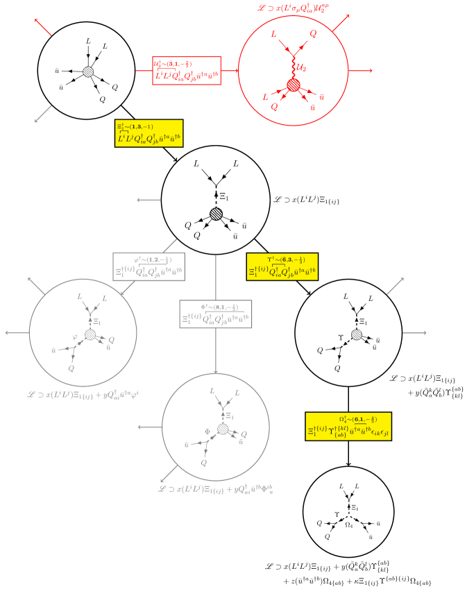
Figure 3: The graph visualises our completion procedure by showing some of the possible ways to explode the operator $\mathcal{O}_{12a\delta}=L^{i}L^{j}Q^{\dagger}_{ia}Q^{\dagger}_{jb}\bar{u}^{\dagger a}\bar{u}^{\dagger b}$. The options are only followed to a fully UV-complete model on one branch, shown in bold with yellow edge labels. In each step groups of fields are contracted at a vertex, fixing the properties of the exotic field as well as the structure of the term describing the interaction, shown alongside each diagram. The effective operator is gradually opened up until each vertex in the diagram corresponds to a term with mass-dimension $d\leq 4$. Opening up the operator fully requires repeating this procedure for all possible contractions. In this case this includes other scalar-only completions and scalar-plus-fermion models. We also show steps that we choose to forbid in our approach in red, like the vector contraction giving rise to the vector leptoquark $\mathcal{U}_{2}$ in the figure. Flavour indices have been suppressed.

Given an effective operator, we have established a simple rule for reducing it to a renormalisable interaction through a processes of contracting fields into each other, corresponding diagrammatically to pairing the fields off into Yukawa or scalar interaction vertices according to a system of rewrite rules. Applying these groupings in all possible ways and following quantum numbers through index structure allows one to efficiently write down not only the particle content generating the operator at tree-level, but also the pertinent interaction terms in the Lagrangian. In the next section, we discuss how to expand this rule to reducing operators containing derivatives.

3.2 Tree-level completions of derivative operators

In the following we broaden the discussion to exploratory model building through effective operators containing (covariant) derivatives and field-strength tensors. We begin by summarising the main results of this section. We argue that (if only scalars and fermions are introduced) a large class of such operators do not contribute new completions to the pool of models. That is, models derived from these operators could be found by opening up operators without derivatives and field strengths. With notable exceptions, it is usually sufficient to study only single-derivative operators. Some of the derivative operators also admit fermion-only completions, which are otherwise only found for the Weinberg-like operators Anamiati:2018cuq . The completion of operators containing derivatives has been studied before in the context of $\Delta L=2$ physics delAguila:2011gr ; delAguila:2012nu ; Herrero-Garcia:2016uab , and our work expands on this.

3.2.1 Exploding derivative operators

In our setup, derivatives in effective operators arise at tree-level by the expansions given in Eqs. (24) and (17). It is clear that derivatives occur in one of two ways: (1) in pairs as $D^{2}$ or $X$ from next-to-leading order terms in the EFT expansion, or (2) as single derivatives contracted with fermions ($\not{D}$ in traditional notation) coming about from arrow-preserving fermion propagators. The job of finding the completions of operators containing derivatives is therefore equivalent to enumerating all possible tree graphs with the appropriate external-leg structure including arrow-preserving propagators proportional to momentum for heavy fermion fields and taking powers of momentum from past the leading order in the expansion of all propagators. As in the non-derivative case, the quantum numbers of the heavy fields can then be deduced by imposing Lorentz and gauge invariance at each vertex.

It is not always guaranteed that a tree-level topology with internal fermion and scalar lines exists for an effective operator containing derivatives. This is in contrast to the non-derivative case, where this is guaranteed for all operators of mass dimension larger than four. For example, at dimension seven there are $\Delta L=2$ effective operators like $\bar{d}_{\alpha}\bar{u}^{\dagger}_{\dot{\alpha}}L^{i\beta}D^{\alpha\dot{\alpha}}L_{\beta}^{i}\epsilon_{ij}$ containing four fermions: three with undotted indices and one with a dotted index. In this case there is no tree-level topology that allows a arrow-preserving fermion propagator to give rise to the derivative, and so the operator can only be generated with loops. We call such operators non-explosive. This distinction between tree and loop operators has been discussed in the literature in the context of the dimension-six operators of the SMEFT, see e.g. Arzt:1994gp ; Einhorn:2013kja ; deBlas:2017xtg , and more recently for the dimension-eight operators Craig:2019wmo .

The derivatives originating from arrow-preserving fermion propagators in the UV theory enter the effective Lagrangian through the first term in Eq. (24). Here, the derivative acts on an object with which it shares a contracted index, i.e. it is contracted as $(\mathbf{2},\mathbf{2})\otimes(\mathbf{1},\mathbf{2})=(\mathbf{2},\mathbf{1})$ with the object carrying the index $\dot{\beta}$. This object must be a $(\mathbf{1},\mathbf{2})$-fermion if it comes from a renormalisable interaction, which in our case is uniquely a Yukawa interaction. Thus,

$$\frac{\partial\mathscr{L}^{lh}}{\partial\Pi_{\dot{\beta}}^{\dagger}}=\sum_{i}\psi^{\dagger\dot{\beta}}_{i}\phi_{i},$$ (33)

with $\psi_{i}$ and $\phi_{i}$ defined as in Eq. (27). For example, a structure like $D^{\alpha\dot{\alpha}}\psi_{1}^{\dagger\dot{\beta}}\phi_{1}\epsilon_{\dot{\alpha}\dot{\beta}}$ could enter an effective operator by integrating out a heavy fermion $\Pi$ that couples through $\mathscr{L}\supset\Pi^{\dagger}\psi^{\dagger}_{1}\phi_{1}$. For clarity, the effective Lagrangian looks like

$$\mathscr{L}_{\text{eff}}[\pi] \supset\frac{\partial\mathscr{L}^{lh}}{\partial\Pi_{\beta}}\frac{1}{m_{\Pi}^{2}}D^{\alpha\dot{\alpha}}\frac{\partial\mathscr{L}^{lh}}{\partial\Pi^{\dagger}_{\dot{\beta}}}\epsilon_{\alpha\beta}\epsilon_{\dot{\alpha}\dot{\beta}}+\cdots$$ (34)

$$=\frac{\partial\mathscr{L}^{lh}}{\partial\Pi_{\beta}}\frac{1}{m_{\Pi}^{2}}D^{\alpha\dot{\alpha}}\left(\psi_{1}^{\dagger\dot{\beta}}\phi_{1}+\cdots\right)\epsilon_{\alpha\beta}\epsilon_{\dot{\alpha}\dot{\beta}}$$ (35)

in this case. The fields $\phi_{i}$ and $\psi_{i}$ need not be light, and could have arisen from the contraction of fields in a complicated way. For example, $\phi_{1}$ may have come from the contraction of two light fermions $\phi_{1}\sim\xi_{1}\xi_{2}$. This situation is visualised diagrammatically in Fig. 4(a). The figure shows the $\xi_{i}$ fermions coupling to the heavy $\phi$ propagator, which in turn couples to $\psi_{1}^{\dagger}$ leading to the arrow-preserving fermion propagator for the heavy $\Pi$ carrying momentum $k^{\alpha\dot{\alpha}}$. It is clear from Eq. (35) that the derivative acts on both the fermion and the scalar, reflecting the fact that in the diagram $k$ is the sum of the $\psi$ and $\phi$ momenta. So, derivatives acting on fermions or scalars can be grouped off into a Yukawa interaction in this way, leaving a arrow-preserving fermion propagator in their wake. This corresponds to the replacement rules

$$\wick{D^{\alpha\dot{\alpha}}(\c{\psi}^{\dagger}_{\dot{\alpha}})\c{\phi}}\to\Pi^{\alpha},\qquad\wick{D^{\alpha\dot{\alpha}}(\c{\psi}^{\dagger}_{\dot{\alpha}}\c{\phi})}\to\Pi^{\alpha},\qquad\wick{D^{\alpha\dot{\alpha}}(\c{\phi})\c{\psi}^{\dagger}_{\dot{\alpha}}}\to\Pi^{\alpha}.$$ (36)

We highlight that the arrow-preserving propagator implies that only one chirality of the Dirac fermion $\Pi$ is necessary for LNV in these models. However, we still only work with vector-like fermions in our completions to guarantee anomaly cancellation and straightforwardly give them large masses.

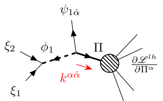
(a)

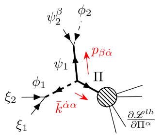
(b)

Figure 4: (a) The diagram shows an example opening of an operator containing at least one derivative. The derivative can be understood as arising from the leading-order term in the expansion of the arrow-preserving fermion propagator, emphasised in the diagram. As shown, the fields $\xi_{i}$ and $\psi_{1}$ are external and therefore light, but in general they could themselves be heavy propagators. (b) The case where the fermion $\psi_{1}$ is heavy, coupling to the light fields $\psi_{2}$ and $\phi_{2}$. The $\sigma$-matrix structure of the propagators is in accordance with the conventions of Ref. Dreiner:2008tw . Here, the Lorentz structure is such that the momenta are contracted, which arises from contractions of derivatives which share one contracted index.

In an effective operator the derivative may act on a fermion with which it does not share a contracted index. For example, in the model shown in Fig. 4(a), the effective operator at the low scale looks something like

$$D^{\beta\dot{\beta}}(\xi^{\alpha}_{1}\xi_{2\alpha}\psi^{\dagger}_{1\dot{\beta}})\frac{\partial\mathscr{L}^{lh}}{\partial\Pi^{\beta}}=D^{\beta\dot{\beta}}(\xi^{\alpha}_{1})\xi_{2\alpha}\psi^{\dagger}_{1\dot{\beta}}\frac{\partial\mathscr{L}^{lh}}{\partial\Pi^{\beta}}+\cdots$$ (37)

although as long as the operator is generated at tree-level, the term with the derivative acting on $\psi^{\dagger}$ will always also be present as long as it is not removed by a field redefinition involving its classical EOM. Our approach is the following: act the derivative in all possible ways on the fields constituting the effective operator and discard the topologies in which a contraction like $\wick{(D^{\alpha\dot{\alpha}}\c{\psi}_{1}^{\beta})\c{\phi}}$ is made. After a UV-complete model is derived, the operator it implies will still have the form of the one on the left-hand side of Eq. (37), so no information is lost. This implies the rules

$$\wick{(D^{\alpha\dot{\alpha}}\c{\psi}^{\beta})\c{\phi}}\to\text{\char 55},\qquad\wick{(D^{\alpha\dot{\alpha}}\c{\psi}^{\beta}\c{\phi})}\to\text{\char 55},\qquad\wick{(D^{\alpha\dot{\alpha}}\c{\phi})\c{\psi}^{\beta}}\to\text{\char 55},\qquad\wick{(D^{\alpha\dot{\alpha}}\c{\phi}_{1})\c{\phi}_{2}}\to\text{\char 55}\ .$$ (38)

The first parentheses of Eqs. (24) and (17) contribute powers of $D^{2}$ or $X$ to operators in the effective Lagrangian. They contribute the rules

$$\wick{(D^{\alpha\dot{\alpha}}\c{\psi}_{1}^{\beta})(D_{\alpha\dot{\alpha}}\c{\psi}_{2\beta})}\to\Phi^{\dagger},\quad\wick{(D^{\alpha\dot{\alpha}}\c{\phi}_{1})(D_{\alpha\dot{\alpha}}\c{\phi}_{2})}\to\Phi^{\dagger}$$ (39)

$$\wick{(D^{\alpha\dot{\alpha}}\c{\psi}^{\beta})(D_{\alpha\dot{\alpha}}\c{\phi})}\to\bar{\Psi}^{\beta},\quad\wick[positions={-1,1},offset=1em]{(D^{\alpha\dot{\alpha}}\c{2}\phi_{1})(D_{\alpha\dot{\alpha}}\c{1}{\c{2}\phi_{2}})\c{1}\phi_{3}}\to\Phi^{\dagger}$$

to those discussed previously. We intend these to stand in for similar rules like e.g. $\wick{\c{\phi}_{1}\Box\c{\phi}_{2}}$ as well. For the field-strength contractions, there is the additional requirement that one or both of the fields in the contraction be charged under the corresponding gauge interaction, but these cannot be contracted into a gauge singlet, since the field-strength tensor comes about from the anticommutator of the covariant derivatives acting on the exotic fermion. These rules are

$$\contraction[1ex]{}{\psi}{{}^{\beta}}{X}\bcontraction[1.3ex]{\psi^{\beta}}{X}{{}_{\alpha\mathsf{j}}^{\mathsf{i}\beta}}{\phi}\psi^{\alpha}_{\mathsf{i}}{X_{\alpha\mathsf{j}}^{\mathsf{i}\beta}}\phi\to\bar{\Psi}^{\beta}_{\mathsf{j}},\quad\contraction[1ex]{}{\phi}{}{X}\bcontraction[1.3ex]{\phi}{X}{{}_{\alpha}^{\beta}}{\phi}\phi{X_{\alpha}^{\beta}}\phi\to\text{\char 55},\quad\contraction[1ex]{}{\psi}{{}^{\beta}}{X}\bcontraction[1.3ex]{\psi^{\beta}}{X}{{}_{\alpha\mathsf{j}}^{\mathsf{i}\beta}}{\phi}\psi^{\alpha}_{\mathsf{i}}{X_{\alpha\mathsf{j}}^{\mathsf{i}\beta}}\phi^{\mathsf{j}}\to\text{\char 55},\quad$$ (40)

where $\mathsf{i}$ and $\mathsf{j}$ stand in for fundamental indices of $\mathrm{SU}(2)_{L}$, $\mathrm{SU}(3)_{c}$, or no indices at all for the field-strength tensor of $\mathrm{U}(1)_{Y}$.

Operators with derivatives coming about as this way, i.e. as $D^{2}$ or $X$, are often redundant from the perspective of model discovery, since they imply the existence of the leading-order operator in which these derivatives do not appear. Thus, the tree-level completions of these operators can be found by studying the lower-dimensional operators without those derivatives or field-strength tensors. It may however be the case that the leading-order operator is absent, in which case these operators may be important. For the $n_{f}=3$ SMEFT with one Higgs doublet, we conjecture this can only come about from operators with a structure like

$$\mathcal{O}^{\mu}H^{i}\partial_{\mu}H^{j}\epsilon_{ij},$$ (41)

which vanishes when the derivative is removed. (Similar structures like $L^{i}_{r}L^{j}_{s}\epsilon_{ij}$ are non-vanishing since there is an additional space of flavour indices to carry the antisymmetry.) This exception does not apply to the case of field-strength tensors, since $[X^{\mu\nu},H]=0$ for all field strengths $X$. This is the justification for our earlier comments that operators containing field-strength tensors are not interesting from the perspective of model discovery.

The replacement rules given in Eq. (39) do not exhaust the possible Lorentz-structures for two derivatives, scalars and fermions. The additional structures involve single indices contracted between the derivatives, and others contracted into fermions. Diagrammatically, we find that these combinations come about from fermion lines containing two arrow-preserving propagators, each contributing a factor of momentum. This would be the case, for example, if $\psi$ in Fig. 4 were a heavy arrow-preserving propagator, as shown in Fig. 4(b). Here the rules are

$$\wick{(D^{\alpha\dot{\alpha}}\c{\psi}_{1\alpha})(D^{\beta\dot{\beta}}\c{\psi}_{2\beta})\epsilon_{\dot{\alpha}\dot{\beta}}}\to\Phi^{\dagger},\quad\wick{(D^{\alpha\dot{\alpha}}\c{\psi})(D^{\beta\dot{\beta}}\c{\phi})\epsilon_{\dot{\alpha}\dot{\beta}}}\to\bar{\Psi}^{\beta},\quad\text{other combinations}\to\text{\char 55}.$$ (42)

In summary, exploding derivative operators can lead to novel models that would not be found by exploding non-derivative operators. We have already seen that this happens when a structure such as Eq. (41) is present in the operator. It can also happen when the presence of an odd number of derivatives allows new topologies with novel chirality structures. The presence of an even number of derivatives implies either that the derivatives arose as $D^{2}$ or $X$, which usually do not contribute new models, or else from the contractions of structures like those in Eq. (42). It is clear from Fig. 4(b) that in such cases, the two arrow-preserving fermion propagators can be replaced with arrow-violating propagators, and indeed these will generically be present since we work with vector-like fermions. So, with the exception of operators with structures like Eq. (41), studying single derivative operators is sufficient for model discovery.

3.2.2 Derivative operator examples

Among the simplest derivative operators in the $\Delta L=2$ SMEFT is the dimension seven operator

$$\mathcal{O}_{D3}=L^{i}_{\alpha}\bar{e}^{\dagger}_{\dot{\beta}}H^{j}(DH)^{\alpha\dot{\beta}k}H^{l}\epsilon_{ij}\epsilon_{kl}$$ (43)

which we use as a paradigm for showing how single-derivative operators can be opened up. We note that the operator’s tree-level completions have also been discussed in Ref. delAguila:2012nu . The placement of the derivative on the Higgs field is enforced by the unique $\mathrm{SU}(2)_{L}$ contraction. This is not generally true, and the derivative should be acted in all possible ways if it can be. The contraction of $(DH)$ into another Higgs is forbidden by Eq. (38). Thus, the $(DH)$ must be contracted into a fermion. The options are

$$\wick{\c{L}^{i}_{\alpha}(D{\c{H}})^{\alpha\dot{\beta}k}}\epsilon_{ij}\epsilon_{kl}\sim\Sigma^{\dagger\dot{\beta}}_{jl}\quad\text{ and }\quad\wick{\c{\bar{e}}_{\dot{\beta}}^{\dagger}{(D{\c{H}})^{\alpha\dot{\beta}k}}}\sim\bar{\Delta}_{1}^{\alpha k}$$ (44)

with the Dirac fermion $\Delta_{1}+\bar{\Delta}_{1}^{\dagger}\sim(\mathbf{1},\mathbf{2},-\tfrac{1}{2})$ transforming like $L$ under $G_{\text{SM}}$. The field $\Sigma$ is the protagonist in the type-III seesaw model, and further contractions on the resulting operator $\Sigma^{\dagger}_{jl}\bar{e}^{\dagger}H^{j}H^{l}$ lead to the models $\{\Sigma,\Delta_{1}+\bar{\Delta}^{\dagger}_{1}\}$ (from $\wick{\c{\bar{e}^{\dagger}}\c{H}}$) and $\{\Sigma,\Xi_{1}\}$ (from $\wick{\c{H}\c{H}}$) in that case. The second option in Eq. (44) leads to the operator $L^{i}\Delta_{1}^{k}H^{j}H^{l}\epsilon_{ij}\epsilon_{jl}$, which is the Weinberg operator with the second $L$ replaced with the exotic vector-like lepton. This contraction is illustrated diagrammatically in Fig. 5(a). It thus implies the same completions as $\mathcal{O}_{1}$, each along with $\Delta_{1}+\bar{\Delta}^{\dagger}_{1}$. This is expected since $\bar{e}^{\dagger}(DH)$ transforms like $L$. There are then a total of five completions, but four models, since two have the same particle content: $\{\Sigma,\Delta_{1}+\bar{\Delta}^{\dagger}_{1}\}$. In Fig. 5(b) we show how this can be seen as coming about from the fact that the chirality structure of the diagram allows two positions for the arrow-preserving fermion propagator. Note that this is not the case for the completion with the singlet fermion $N$. Interestingly, there are two fermion-only models found: $\{N,\Delta_{1}+\bar{\Delta}^{\dagger}_{1}\}$ and $\{\Sigma,\Delta_{1}+\bar{\Delta}^{\dagger}_{1}\}$. Both of them contain seesaw fields, which is consistent with the proof of Ref. Klein:2019iws that models containing two exotic fermion fields must contain one of $N$ or $\Sigma$ if they violate lepton-number by two units. Since the structure of the operator $\mathcal{O}_{D3}$ is unique, there is no work to be done in writing down the organic operator generated by these models at the low scale.

(a)

(b)

Figure 5: (a) An intermediate topology representing the operator $\mathcal{O}_{D3}$ with all heavy fields except $\Delta_{1}$ integrated out. The contraction $\bar{e}^{\dagger}H\sim\Delta^{\dagger}_{1}$ gives rise to an effective operator similar to the Weinberg operator $\mathcal{O}_{1}$, shown in blue. This branch of the completion tree therefore involves models featuring $\Delta_{1}$ along with one of the seesaw fields. (b) The model with field content $\{\Sigma,\Delta_{1}+\bar{\Delta}^{\dagger}\}$ arises from two similar diagrams, shown here. These correspond to the two ways the arrow-preserving and arrow-violating fermion propagators can be placed in the graphs for this furnishing of the topology.

We move on to a two-derivative operator example by studying a completion of

$$\mathcal{O}_{18d}=L^{i}L^{j}H^{k}H^{l}(D^{\mu}H)^{m}(D_{\mu}\tilde{H})^{n}\epsilon_{ij}\epsilon_{km}\epsilon_{ln},$$ (45)

which has the property that it vanishes when the derivatives are removed. (Note that, comparing to the operator in Table LABEL:tab:long, the first derivative has been moved onto a Higgs field.) Applying the only allowed replacement rule on the derivatives first implies the presence of the real triplet scalar $\Xi\sim(\mathbf{1},\mathbf{3},0)_{S}$ in the theory

$$\wick{L^{i}L^{j}H^{k}H^{l}(D^{\mu}\c{H})^{m}(D_{\mu}\c{\tilde{H}})^{n}}\epsilon_{ij}\epsilon_{km}\epsilon_{ln}\to L^{i}L^{j}H^{k}H^{l}\Xi^{mn}\epsilon_{ij}\epsilon_{km}\epsilon_{ln}.$$ (46)

From here there are a number of choices. We choose to look at a particular scalar-only completion involving the unit-hypercharge isosinglet scalar present in the Zee model $\mathcal{S}_{1}\sim(\mathbf{1},\mathbf{1},1)$:

$$\wick{\c{L}^{i}\c{L}^{j}H^{k}H^{l}\Xi^{mn}}\epsilon_{ij}\epsilon_{km}\epsilon_{ln}\to\mathcal{S}^{\dagger}_{1}H^{k}H^{l}\Xi^{\dagger}_{kl},$$ (47)

implying the interaction Lagrangian

$$\mathscr{L}_{\text{int}}\supset x_{[rs]}L_{r}L_{s}\mathcal{S}_{1}+\kappa H^{i}\tilde{H}^{j}\Xi_{\{ij\}}+\lambda\mathcal{S}_{1}\Xi^{ij}H^{\dagger}_{i}H^{\dagger}_{j}+\text{h.c.}$$ (48)

This model was studied in Ref. Law:2013dya and identified as the simplest neutrino mass model according to their assumptions. It has remarkably few free parameters since the scalar $\Xi$ does not have Yukawa couplings to SM fermions, and the couplings of $\mathcal{S}_{1}$ to leptons are antisymmetric in flavour. As in the minimal Zee–Wolfenstein scenario Wolfenstein:1980sy , this model implies a neutrino-mass matrix with zeros down the diagonal and is therefore incompatible with neutrino oscillation data He:2003ih . It is, however, a good example of how interesting models can be missed when overlooking operators with derivatives in this model-building framework. The model generates the following combination of basis operators at the low scale

$$\mathcal{O}^{[rs]}_{\mathcal{S}_{1}+\Xi}=(L_{r}^{i}L_{s}^{j})H^{k}H^{l}\Box(H^{m}\tilde{H}^{n})\epsilon_{ij}\epsilon_{km}\epsilon_{ln}.$$ (49)

Note that the operator is already symmetric under the interchage $m\leftrightarrow n$, so another structure need not be added.

3.3 An algorithm for model building

With our basic completion recipe established, in the following we outline the procedures we use to build the UV models that generate the operators listed in Table LABEL:tab:long, along with relevant metadata: the tree-level diagrams and the models’ Lagrangians. The methods are presented as they are implemented in our example code neutrinomass2020 .

We use a computational representation for tensors representing fields transforming as irreducible representations of $\mathrm{SU}(2)_{+}\otimes\mathrm{SU}(2)_{-}\otimes G_{\text{SM}}$ built on top of the SymPy package 10.7717/peerj-cs.103 for symbolic computation in Python, as well as BasisGen Criado:2019ugp for group-theory functionality. The code implements the Butler–Portugal algorithm butler1991 ; MANSSUR_2002 for obtaining the canonical form of tensorial expressions, which we use to simplify operators and compare them for equality. Strings of fields and their derivatives representing gauge- and Lorentz-invariant effective operators are dressed with $\epsilon$ and $\delta$ tensors to form all possible invariants. In our specific case, the content of these operators is constructed directly by taking the product of all field combinations and keeping only those that contain a singlet part in the decomposition. We checked this against results from the Hilbert series, projecting out the $\Delta L=2$ component for the pertinent operators, and removing the spurions accounting for redundancies from field redefinitions involving the classical EOM and IBP. For our study of the $\Delta L=2$ operators, since we are interested in model discovery, we excluded derivative operators that are non-explosive along with those that contain field-strength tensors and contracted pairs of derivatives that do not lead to a vanishing structure upon removal.

In practice we start with a template pattern of contractions corresponding to the topologies that can accommodate the field content of the operators at tree-level. These are generated using FeynArts Hahn:2000kx through Mathematica, and filtered for isomorphism with graph-theory tools igraph2006 ; the_igraph_core_team_2020_3774399 ; szabolcs_horvat_2020_3739056 ; SciPyProceedings_11 . These templates provide the order and pattern of contractions for classes of operators based on the number of scalars and fermions they contain. Since no distinction is made at this level between $(\mathbf{2},\mathbf{1})$- and $(\mathbf{1},\mathbf{2})$-fermions, for some operators only a subset of these templates will be relevant for our purposes, since some contractions may always imply Proca fields. These templates are used to open up the operator with the assumptions and methods presented in Sec. 3. Every time a replacement rule is applied, the Feynman graph information is updated and a Lagrangian term is generated as described in Sec. 3.1.1. After the procedure is finished, the full Lagrangian of the model can be generated in the same way as the input effective operators, described above.

We keep track of the quantum numbers of the heavy fields so as to be economic with exotic degrees of freedom, while still providing some flexibility in the model database. Concretely, if a field arises from a contraction whose corresponding term has already appeared in the Lagrangian, the two associated exotic fields are identified. If two fields come about from different contractions but share the same quantum numbers they are distinguished, since it may be possible that some symmetry would forbid one term but not the other. The choice to identify fields not only reduces the number of fields in each model, but may also reduce the total number of completions for a given operator. This is due to couplings between exotic fields that vanish in the absence of some exotic generational structure. For example, $\phi^{i}\phi^{j}\epsilon_{ij}=0$ for some exotic isodoublet $\phi$, or $\eta^{a}\eta^{b}\eta^{c}\epsilon_{abc}=0$ for a colour-triplet $\eta$.

We have attempted to validate our example code against many results in the literature. We have been able to reproduce the results of Refs. delAguila:2012nu ; Cai:2014kra ; Herrero-Garcia:2016uab ; deBlas:2017xtg ; deGouvea:2019xzm , which give systematic listings of models that generate effective operators at tree-level. Ref. deBlas:2017xtg provides a UV dictionary for the dimension-six SMEFT. Validation of these results first required the adaptation of the dimension-six operators to something analogous to the overcomplete spanning set of type-3 operators used here. The entire process in this case—including generating the set of operators, finding the completions and matching examples back onto the Warsaw basis—is provided as an interactive notebook accompanying our example code. We note that such matching calculations can also be automated with the help of automated tools Criado:2017khh ; Bakshi:2018ics . For the other studies mentioned, we provide our validation of their results along with our example code.

4 Neutrino mass model building

Up until now we have tried to keep the discussion of exploding operators general, but in this and following sections we specialise to the case of opening up operators to build radiative models of Majorana neutrino mass. We discuss the process of turning $\Delta L=2$ operators into neutrino self-energy graphs, the tree-level topologies of the operators, and the methods we use to ensure a given model’s contribution to the neutrino mass is the dominant one.

4.1 Operator closures and neutrino-mass estimates

For operators other than the Weinberg-like ones, neutrino masses are necessarily generated at loop level. The fields of the $\Delta L=2$ operator need to be looped off using SM interactions in such a way that a Weinberg-like operator is generated after the SM fields are integrated out. We call this the operator closure and it represents the mixing between the $\Delta L=2$ operator and the Weinberg-like ones. Examples of $\Delta L=2$ operator closures are given in Table LABEL:tab:example-closures, and these are referred to throughout this section. The closure provides enough information to know the number of loops in the neutrino self-energy graph (since the $\Delta L=2$ operator is generated at tree level) and to estimate the scale of the new physics underlying the operator. We automate the operator-closure process by applying the methods discussed below through a pattern-matching algorithm krebber2018 ; krebber2017nonlinear . The program is a part of our public example-code repository.

Current neutrino oscillation data provide a lower bound on the mass of the heaviest neutrino, coming from the measured atmospheric mass-squared difference $\Delta m^{2}_{\text{atm}}\approx(0.05\text{ eV})^{2}$ nufitweb ; Esteban:2018azc . We take the neutrino-mass scale $m_{\nu}\approx 0.05\text{ eV}$, so that the new-physics scale is bounded above by the implied scale we estimate for each operator. This is derived by estimating the loop-level operator closure diagrams. In our case we are interested in estimating the scale of the neutrino mass in the UV models generating the operator, rather than the calculable loop-level contributions to the neutrino mass in the EFT. We associate a factor of $(16\pi^{2})^{-1}\approx 6.3\cdot 10^{-3}$ with each loop and assume unit operator coefficients for the non-renormalisable $\Delta L=2$ vertices. We take the SM Yukawa couplings to be diagonal and include factors of $g\approx 0.63$ appropriately for interaction vertices involving $W$ bosons. Neutrino-mass matrices proportional to Yukawa couplings will be dominated by the contributions from the third generation of SM fermions in the absence of any special flavour hierarchy in the new-physics couplings. For this reason, we consider only the effects of third-generation SM fermions in our estimates, but mention that our program can be straightforwardly extended to accommodate the general case where light-fermion Yukawas and off-diagonal CKM matrix elements appear in the neutrino-mass matrix. For derivative-operator closures, we can include the $W$ boson from the covariant derivative if it is present and necessary to correctly close off the diagram. Otherwise, the vertex should come with an additional factor of momentum. We work in the Feynman gauge to avoid spurious factors of $\Lambda$ in the neutrino-mass estimates delAguila:2012nu . The overall scale-suppression of the neutrino mass is determined by the Weinberg-like operator generated at the low scale. In most cases, this is the dimension-five operator $\mathcal{O}_{1}$, which implies $m^{\mathcal{O}_{1}}_{\nu}\sim v^{2}/\Lambda$. Closures leading to the loop-level generation of $\mathcal{O}_{1}^{\prime}$ and $\mathcal{O}_{1}^{\prime\prime}$ can also be found, and these naively imply a significant suppression of the neutrino mass compared to the $\mathcal{O}_{1}$ case: $m^{\mathcal{O}_{1}^{\prime}}_{\nu}\sim v^{4}/\Lambda^{3}$ and $m^{\mathcal{O}_{1}^{\prime\prime}}_{\nu}\sim v^{6}/\Lambda^{5}$. However, a diagram with additional Higgs loops can always be drawn to recover the Weinberg operator at the low scale. Despite the additional loop suppression, these diagrams will dominate over those generating $\mathcal{O}_{1}^{\prime}$ and $\mathcal{O}_{1}^{\prime\prime}$ as long as $\Lambda\gtrsim 4\pi v\approx$2.2\text{\,}\mathrm{TeV}$$ Babu:2001ex ; deGouvea:2007qla .

It is still true that higher-dimensional operators typically imply smaller neutrino masses. There are two main reasons for this. First, the number of loops required for the closure of the operator generally increases with increasing mass dimension. Second, operators containing more fields imply neutrino self-energy diagrams containing more couplings. Many of these are SM Yukawas which (with the exception of $y_{t}$) are small and tend to suppress the neutrino mass, despite the contributions being dominated by the third generation. Non-minimal choices such as small exotic Yukawa couplings or hierarchical flavour structures in the operator coefficients can also lead to additional suppression of the neutrino mass, and in turn of the implied scale of the new physics.

In Fig. 6 we show the new-physics scales $\Lambda$ associated with neutrino-mass generation from the $\Delta L=2$ operators in the SMEFT up to dimension 13, assuming unit operator coefficients and the dominance of third-generation couplings. We separate single-derivative operators from those that contain no derivatives, and choose not to include operators containing more than one derivative in the figure. This is because these operators most often arise at next-to-leading order in the EFT expansion, and therefore usually imply a neutrino-mass scale identical to that of lower-dimensional operators. The dimension-eleven operators with derivatives as well as the dimension-13 operators are constructed only as products of lower-dimensional ones, making the set of operators incomplete. We highlight that similar kinds of product operators at dimensions eleven and nine do not imply special values for the estimated neutrino-mass scale or $\Lambda$, and therefore we expect the results to be representative of the situation up to dimension 13. From the figure, it is clear that there is a trend towards smaller values of $\Lambda$ with increasing mass dimension. By dimension 13, the implied new-physics scale is between $1$ and $100~{}\text{TeV}$ for most operators. It seems to be the case that the most constrained closures are generally those of non-derivative operators.

Table 3: The table shows an assortment of $\Delta L=2$ operator closures, displaying a number of paradigmatic motifs. We represent flavour indices in a sans-serif typeface here to avoid confusion with subscripts labelling the Yukawa couplings. The expressions given for $m_{\nu}^{\textsf{rs}}$ needs to be symmetrised in rs, something we do not explicitly indicate in the table. These expressions carry flavour indices in alphabetical order on the fields as they appear in Table LABEL:tab:long. Here $\kappa$ represents the operator coefficient, $V$ is the CKM matrix and $y^{\textsf{r}}_{e,u,d}$ are the diagonal electron, up-type and down-type Yukawa couplings in the SM. A number of operators require an external electron to be converted into a neutrino. This often necessitates the introduction of a $W$ boson or an unphysical charged Higgs $H^{+}$. Operator $\mathcal{O}_{8}$ generates the dimension-seven analogue of the Weinberg operator with the two-loop diagram shown. (There is a lower order diagram with an $H^{+}$ in place of the $W$ that happens to vanish Babu:2010vp .) A three-loop diagram in which two of the external Higgs lines are looped off leads to mixing with the Weinberg operator. Operator $\mathcal{O}_{76}$ generates the dimension-nine operator $LLHH(H^{\dagger}H)^{2}$, and hence five- and six-loop diagrams are also implied. There is usually more than one choice about where to attach the $W$ boson if one is present in a diagram, and the additional diagrams with the $W$ connecting in other possible ways are left implicit.

Operator	Diagram	$m_{\nu}^{\textsf{rs}}$
$4b$		$\displaystyle\kappa_{\textsf{[rs]tt}}\frac{g^{2}y_{u}^{\textsf{t}}}{(16\pi^{2})^{2}}\frac{v^{2}}{\Lambda}$
$8$		$\displaystyle\kappa_{\textsf{rstu}}V_{\textsf{tu}}\frac{g^{2}y_{e}^{\textsf{s}}y_{u}^{\textsf{t}}y_{d}^{\textsf{u}}}{(16\pi^{2})^{2}}\frac{v^{2}}{\Lambda}\left(\frac{v^{2}}{\Lambda^{2}}+\frac{1}{16\pi^{2}}\right)$
$D3$		$\displaystyle\kappa_{\textsf{rs}}\frac{y_{e}^{\textsf{s}}}{16\pi^{2}}\frac{v^{2}}{\Lambda}$
$11b$		$\displaystyle\kappa_{\textsf{rstutu}}\frac{y_{d}^{\textsf{t}}y_{d}^{\textsf{u}}}{(16\pi^{2})^{2}}\frac{v^{2}}{\Lambda}$
$76$		$\displaystyle\kappa_{\textsf{rstuvw}}V_{\textsf{tv}}V_{\textsf{uw}}\frac{g^{4}y^{\textsf{r}}_{e}y^{\textsf{s}}_{e}y_{u}^{\textsf{t}}y_{u}^{\textsf{u}}y_{d}^{\textsf{v}}y_{d}^{\textsf{w}}}{(16\pi^{2})^{4}}\frac{v^{2}}{\Lambda}\left(\frac{v^{2}}{\Lambda^{2}}+\frac{1}{16\pi^{2}}\right)^{2}$
$47a$		$\displaystyle\kappa_{\textsf{rstuvw}}\frac{1}{(16\pi^{2})^{2}}\frac{v^{2}}{\Lambda}$
$56$		$\displaystyle\kappa_{\textsf{rsttvv}}\frac{y_{e}^{\textsf{s}}y_{d}^{\textsf{t}}}{(16\pi^{2})^{3}}\frac{v^{2}}{\Lambda}$

We note that at dimension eleven it begins to become clear that the neutrino-mass estimates associated with a category of operators remain large. These operators include $\mathcal{O}_{47a}$, whose closure is shown in Table LABEL:tab:example-closures, and 44 others like it which have loops that contain no connecting Higgs, and therefore no additional suppression from SM Yukawa couplings. These operators have the form

$$\mathcal{O}_{1}\cdot\prod_{i=1}^{n}\psi_{i}^{\dagger}\psi_{i},$$ (50)

where $\psi_{i}$ are SM fermion fields, and imply

$$m_{\nu}\sim\kappa\frac{1}{(16\pi^{2})^{n}}\frac{v^{2}}{\Lambda},$$ (51)

with $\kappa$ the operator coefficient. The loop suppression becomes too great to meet the atmospheric bound at $n=6$. Although five loops are viable in the absence of any other suppression, the operators $\mathcal{O}_{1}\cdot\prod_{i=1}^{5}(\psi_{i}^{\dagger}\psi_{i})$ cannot form a Lorentz-singlet without a derivative. This suggests that dimension-21 operators of the form

$$LLH(\partial^{\mu}H)\cdot(\psi_{0}\sigma_{\mu}\psi_{0}^{\dagger})\prod_{i=1}^{4}\psi_{i}^{\dagger}\psi_{i}$$ (52)

are the highest-dimensional operators leading to phenomenologically viable neutrino masses. They require new physics below $\sim 6~{}\text{TeV}$. All of the tree-level topologies associated with the structure in Eq. (52) imply that the neutrino mass depends on the product of nine or more dimensionless couplings. It is clear from Fig. 6 that these operators are outliers, and the associated new-physics scale is already heavily constrained by dimension 13 for most.

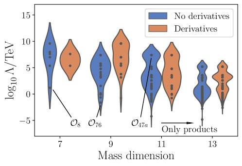
Figure 6: The figure shows smoothed histograms of the number of operators that have an estimated upper bound of $\Lambda$ on the new-physics scale. Black dots generally represent more than one operator. The strips are broken up by mass dimension and whether the operators contain derivatives or not. We assume unit operator coefficients and the dominance of third-generation SM-fermion contributions in the closure diagrams. Operators containing no derivatives (blue) are separated from those containing one derivative (orange). Those containing more than one derivative are not included in the figure, since in most cases these come about at next-to-leading order in the EFT expansion, and therefore imply the same $\Lambda$ values as the lower-dimensional operator with two fewer derivatives. The dimension-eleven operators containing one derivative and all of the dimension-13 operators shown are constructed from the lower-dimensional operators in our listing only as products. This means that the set of operators plotted above that do not feature in Table LABEL:tab:long are incomplete. However, we do not find that similar product-type operators at dimensions nine and eleven give special estimates for the neutrino mass or $\Lambda$, and so we expect these results to be representative of the true situation up to mass-dimension 13. The general decrease in $\Lambda$ with increasing operator mass dimension is evident in the figure. The most suppressed closures tend to be of non-derivative operators. By mass-dimension eleven it becomes clear that a class of operators, those with the structure shown in Eq. (50), are less suppressed than the rest.

Estimates for the neutrino mass for the majority of the $\Delta L=2$ operators without derivatives have been given previously in Ref. deGouvea:2007qla . Those that we present here differ in two ways:

1. We aim to estimate the contribution to the neutrino mass implied by the completions of the operator, not the operator alone. This means, for example, that we do not need more loops of gauge bosons to provide additional factors of momentum on fermion loops with no mass insertions, since it is implicit that the appropriate factors of momentum will arise at higher orders in the EFT expansion. Such arrow-preserving loops, as shown in the closures of $\mathcal{O}_{47a}$ and $\mathcal{O}_{56}$ in Table LABEL:tab:example-closures, vanish by even–odd parity arguments absent these higher-order contributions deGouvea:2007qla . Indeed, in UV models built from these operators the additional gauge-boson loops are not necessary Angel:2012ug ; Gargalionis:2019drk . This means that for operators such as $\mathcal{O}_{47a}$ and $\mathcal{O}_{56}$, our neutrino-mass estimates are enhanced with respect to those presented in Ref. deGouvea:2007qla by $16\pi^{2}/g^{2}$.

2. In some cases, operators containing a factor of $\bar{u}^{\dagger}\bar{d}$ require a closure with $W$ bosons rather than $H^{+}$, since the sum of the diagrams with the unphysical Higgs fields vanishes Babu:2010vp . The situation is shown in Fig. 7 for a general one-loop case of this phenomenon. Ultimately this comes from the relative negative sign in the Lagrangian between the up- and down-type Yukawa interactions:

   $$\mathscr{L}_{\text{Yuk}}\supset y_{u}^{r}V_{rt}d_{t}\bar{u}_{r}H^{+}-y_{d}^{r}V_{tr}\bar{d}^{\dagger}_{r}u^{\dagger}_{t}H^{+}\ .$$ (53)

   As shown in the Fig. 7, the fermion loop requires a mass insertion on the quark line to which the $H^{+}$ does not connect, making both loops proportional to $y_{u}y_{d}$ but with differing signs. Care must be taken to ensure that the loop functions are also necessarily the same in cases where this property is used.

It might be possible that, in a similar way to (2) above, the sum of diagrams with different $W$ placements or of the neutrino-flavour-symmetrised diagrams might also lead to additional cancellations which further decrease the upper bound on the new-physics scale. This not a possibility we explore in detail here, but note that similar cancellations have been noted in the literature Gargalionis:2019drk .

Figure 7: For some operators containing $\bar{d}\bar{u}^{\dagger}$ the operator closure involves a motif like that shown in the figure. There is always an additional diagram with the roles of the unphysical Higgs and $H^{0}$ interchanged. Both diagrams are proportional to $y_{u}y_{d}$ but related by a negative sign coming from the couplings of $H^{+}$ to up- and down-type quarks as shown in Eq. (53), and therefore their sum vanishes.

Our estimates for the neutrino mass are provided as symbolic mathematical expressions in our model database. Where possible these been checked against more detailed calculations and UV models in the literature generating the operators to ensure acceptable agreement Duerr:2011zd ; Babu:2009aq ; Babu:2010vp ; delAguila:2012nu ; Cai:2014kra ; Zee:1985id ; Babu:1988ki ; Angel:2013hla ; Gargalionis:2019drk . The predictions for the new-physics scale associated with each operator are provided in Table LABEL:tab:long, along with the number of loops in the closure. Operators for which a range is given for the number of loops are those that generate the dimension-seven or dimension-nine analogues of the Weinberg operator. As touched on above, the additional Higgs fields in these closures can always be closed off, adding more loops to the neutrino self-energy diagram while reducing the overall scale suppression. The contribution with the highest number of loops will dominate for scales $\Lambda\gtrsim 4\pi v$.

We note that in some cases, more insights can be made about the structure of the neutrino-mass matrix from the nature of the operator, even in the general form with which they appear in our classification. For example, there is only one independent Lorentz-structure associated with $\mathcal{O}_{4b}$: $\kappa^{\mathcal{O}_{4b}}_{rstt}(L^{i}_{r}L^{j}_{s}\epsilon_{ij})(Q^{\dagger}_{tk}\bar{u}^{\dagger}_{t})H^{k}$, from which it can be seen that the operator coefficient must be antisymmetric in $rs$ from Fermi–Dirac statistics. It is clear from the diagram associated with the operator in Table LABEL:tab:example-closures that the loop integral will depend on an external lepton flavour, and this dependence can only come from charged-lepton masses, i.e. $I(m_{e}^{r})$. Then the complete expression for the estimated neutrino mass will be something like

$$m_{\nu}^{\{rs\}} \sim\sum_{t}\frac{g_{2}^{2}y_{u}^{t}}{(16\pi^{2})^{2}}\frac{v^{2}}{\Lambda}[\kappa_{[rs]tt}I(m_{e}^{r})+\kappa_{[sr]tt}I(m_{e}^{s})]$$ (54)

$$=\sum_{t}\frac{g_{2}^{2}y_{u}^{t}}{(16\pi^{2})^{2}}\frac{v^{2}}{\Lambda}\kappa_{[rs]tt}[I(m_{e}^{r})-I(m_{e}^{s})],$$ (55)

which implies a neutrino-mass matrix with zeros down the diagonal, similar to that following from the Lagrangian in Eq. (48). Such a texture is disfavoured by neutrino oscillation data. Studying the structure of the neutrino-mass matrices implied by a complete basis of $\Delta L=2$ operators would allow more, similar conclusions to be drawn in a model-independent way. Recently, a complete basis of operators in the SMEFT at dimension nine has been written down Li:2020xlh , and this could facilitate such an effort.

4.2 UV considerations

We now turn to the UV structure of the operators: their completion topologies, the associated neutrino self-energy graphs, and the nature of the exotic fields that feature therein. Central to our study of neutrino mass is the requirement that a model represent the leading contribution to the neutrino mass, a condition we impose through a process of model filtering, also discussed in the present section.

4.2.1 Tree-level completion topologies

The tree-level UV topologies depend on the number of fermions and scalars in the operator, and this is how we choose to label them. Thus, a dimension-eleven operator with two scalars and six fermions has topologies labelled $2s6f_{i}$. We do not distinguish between $(\mathbf{2},\mathbf{1})$- and $(\mathbf{1},\mathbf{2})$-fermions in this classification, and some of these topologies will therefore always imply the existence of heavy vector particles in the completions. In our analysis these models are not considered, but the topologies are still presented here in general. Each topology corresponds to a pattern of contractions in the language of Sec. 3, and sometimes we use this perspective.

We present the different topology types in Table 4 along with peripheral information relating to these. The number of propagators in the diagrams represents an inclusive upper bound on the number of exotic fields allowed in the completions of the associated operators, counting Dirac fermions as one exotic field. In many cases, repetition in the operator’s field content can lead to fewer fields furnishing the internal lines of the diagram, since we identify fields with the same quantum numbers. To avoid clutter we keep the complete gallery of tree-level diagrams in our online example-code repository, and instead only show some of the graphs here. For some topology types the relevant diagrams have already appeared in earlier parts of the paper, and these figures are referenced in the table. We make more specific comments about the topology types by operator mass dimension below.

Topology type	Operators	Topologies	Propagators	Figure
$0s4f$	$2$	1	1	$\hookrightarrow$
$0s6f$	$16$	2	3	2
$1s4f$	$16$	2	2	8(b)
$2s2f$	$7$	1	1	1
$2s4f$	$29$	8	2,3	9(b)
$2s6f$	$137$	35	4,5	11
$3s2f$	$3$	4	1,2	10(b)
$3s4f$	$15$	23	3,4	9(a)
$4s2f$	$8$	10	2,3	8(a)
$5s2f$	$1$	24	2,3,4	10(a)
$5s4f$	$15$	264	4,5,6	$\hookrightarrow$
$6s2f$	$1$	66	3,4,5	$\hookrightarrow$

Table 4: The table shows the topology classes encountered in our operator listing along with related information: the number of pertinent operators, the number of tree-level topologies associated with each topology type, the number of internal lines featuring in the diagrams (given as a range), and the appropriate figure reference in the text. Although there is one $0s4f$ topology, all of the pertinent operators in our listing are non-explosive because they contain derivatives. The symbol $\hookrightarrow$ indicates that we do not present these topologies in this paper; instead, we point the interested reader to our online database and example code for the relevant diagrams. We highlight that although the topologies are labelled only by their field content, the pertinent operators may include one or more derivatives. We point the reader to the main text for a detailed breakdown by mass-dimension of the topologies that are relevant to each operator.

Dimension seven

At dimension seven there are three broad classes of $\Delta L=2$ operators by field-content: $0s4f$, $1s4f$ and $4s2f$ in our classification scheme. Operator $\mathcal{O}_{D1}$ is one of only two $0s4f$ operators in the entire listing, both of which are non-explosive. The Weinberg-like $\mathcal{O}_{1}^{\prime}$ is the only $4s2f$ operator at dimension seven, while there are six $4s2f$ operators: $\mathcal{O}_{2}$, $\mathcal{O}_{3a,b}$, $\mathcal{O}_{4a,b}$ and $\mathcal{O}_{8}$. The UV topologies relevant for the dimension-seven operators are presented in Fig. 8. There are only two tree-level topologies associated with the $1s4f$ operators. One involves two exotic scalars, the other an exotic scalar and a heavy fermion with an arrow-violating propagator line. There are ten topologies associated with the $4s2f$ class, for which the only pertinent operator is $\mathcal{O}_{1}^{\prime}$. Only topology $4s2f_{3}$ is associated with a model that does not contain seesaw fields. Topology $4s2f_{6}$ accommodates up to three exotic scalars and $4s2f_{8}$ allows up to three exotic fermions. Such fermion-only models are expected only for the Weinberg-like operators, in the absence of derivatives. The remaining topologies allow all other combinations up to three fields for the number of exotic scalars and fermions introduced. Radiative neutrino mass from the dimension-seven operators without derivatives was also studied in Ref. Cai:2014kra .

(a)

(b)

Figure 8: (a) The tree-level topologies relevant for the completions of the four-scalar–two-fermion operator $\mathcal{O}_{1}^{\prime}$. Only topology $4s2f_{3}$ leads to a novel completion that does not feature a seesaw field. We point out that topology $4s2f_{8}$ permits fermion-only completions, which are expected only for the Weinberg-like operators in the absence of derivatives. (b) The two tree-level topologies relevant for the completions of the one-scalar–four-fermion dimension-seven operators in Table LABEL:tab:long. The internal fermion line on $1s4f_{2}$ must be arrow-violating for all of the operators we consider.

Dimension nine

At dimension nine there are 79 operators in our catalogue. There are 16 operators containing six fermions, these are $\mathcal{O}_{9}$ through to $\mathcal{O}_{20}$ as well as $\mathcal{O}_{76}$. The relevant tree-level topologies are presented in Fig. 2. There are 15 $3s4f$ operators, most of which have the form $\mathcal{O}_{1}\cdot\mathcal{O}_{\text{SM Yukawa}}$ or $H^{\dagger}H$ times a $1s4f$ dimension-seven operator. These are operators $\mathcal{O}_{5}$ through to $\mathcal{O}_{7}$ as well as $\mathcal{O}_{61}$, $\mathcal{O}_{71}$, $\mathcal{O}_{77}$, $\mathcal{O}_{78}$ and $\mathcal{O}_{8}^{\prime}$. These topologies are shown in Fig. 9(a). There is a single $6s2f$ operator: the Weinberg-like $\mathcal{O}_{1}^{\prime\prime}$. The remaining 47 operators contain derivatives. Those that contain an even number share topologies with dimension-five or dimension-seven operators. These include $\mathcal{O}_{D19}$, a $2s2f$ operator, $\mathcal{O}_{D18}$ and $\mathcal{O}_{D22}$ which are $4s2f$ operators with associated topologies shown in Fig. 8(a), as well as $\mathcal{O}_{D4}$, $\mathcal{O}_{D7}$, $\mathcal{O}_{D13}$ and $\mathcal{O}_{D15}$ for which the $1s4f$ topologies of Fig. 8(b) are relevant. The remaining operators contain an odd number of derivatives. The operators $\mathcal{O}_{D5}$, $\mathcal{O}_{D6}$, $\mathcal{O}_{D8}\text{ -- }\mathcal{O}_{D10}$, $\mathcal{O}_{D12}$, $\mathcal{O}_{D14}$, $\mathcal{O}_{D16}$ and $\mathcal{O}_{D17}$ are of type $2s4f$, implying entirely new topologies, shown in Fig. 9(b). To these we add the $5s2f$ operator $\mathcal{O}_{D20}$ and the $3s2f$ operator $\mathcal{O}_{D21}$, which also have novel structure. Fig. 10(a) and Fig. 10(b) are relevant in this case. For the operators that contain an odd number of derivatives, only the topologies allowing at least one arrow-preserving fermion propagator do not contain exotic Proca fields. Some $3s4f$ and $5s2f$ topologies have the interesting property that they involve exotic fields that couple only to other exotic fields in the diagram. These are the lowest-dimensional operators in our listing having this feature, although this becomes more common at dimension eleven.

We note that the tree-level topologies can also be important in telling which derivative operators might provide novel completions. As discussed in Sec. 3.2.1, many operators containing more than one derivative have no model-discovery utility. These are operators generated past the leading order in the expansion of the heavy propagators in the UV theory, and their completions are always found by exploding the lower-dimensional operators with an even number of fewer derivatives. One way to diagnose such a situation is to check how many arrow-preserving fermion lines are present in the tree-level topologies associated with an operator. If all of the graphs contain fewer such propagators than the number of derivatives in the operator, then any model generating this operator will also generate the corresponding lower-dimensional one. At dimension nine there are seven operator classes that fall into this category. The four operator families $\mathcal{O}_{D4}$, $\mathcal{O}_{D7}$, $\mathcal{O}_{D13}$ and $\mathcal{O}_{D15}$ each contain two derivatives. These operators are identified above as fitting into the $1s4f$ topology class. It is clear from Fig. 8(b) that no two-fermion completions are relevant to this class, and the Lorentz structure of these operators is such that the internal fermion can only by arrow-violating. This suggests that models generating these operators at tree-level will always also generate the derivative-free dimension-seven operators $\mathcal{O}_{2}$, $\mathcal{O}_{3}$, $\mathcal{O}_{4}$ and $\mathcal{O}_{8}$, respectively. There are two three-derivative operators: $\mathcal{O}_{D21}$, of topology class $3s2f$, and $\mathcal{O}_{D11}$, a $0s4f$ operator. The latter is non-explosive and therefore not relevant to a discussion of tree-level model building. The $3s2f$ class admits completions that contain one and two fermions: those associated with topologies $3s2f_{4}$ and $3s2f_{2}$, respectively. In both both cases we find that the operator’s structure allows for only a single arrow-preserving propagator in each diagram. As before, this suggests that $\mathcal{O}_{D21}$ is not interesting for model discovery, and its completions will be found by studying $\mathcal{O}_{D3}$. Finally, there is also one four-derivative operator at dimension nine: the $2s2f$ operator $\mathcal{O}_{D19}$ whose completions coincide with those of the Weinberg operator $\mathcal{O}_{1}$. This means that the only two-derivative operators in our listing that could contribute new completions to the pool of neutrino-mass models are $\mathcal{O}_{D18}$ and $\mathcal{O}_{D22}$. Operator $\mathcal{O}_{D22}$ has the feature that the removal of the derivatives causes the operator to vanish, while this is not true for all of the $\mathrm{SU}(2)_{L}$ structures associated with $\mathcal{O}_{D18}$.

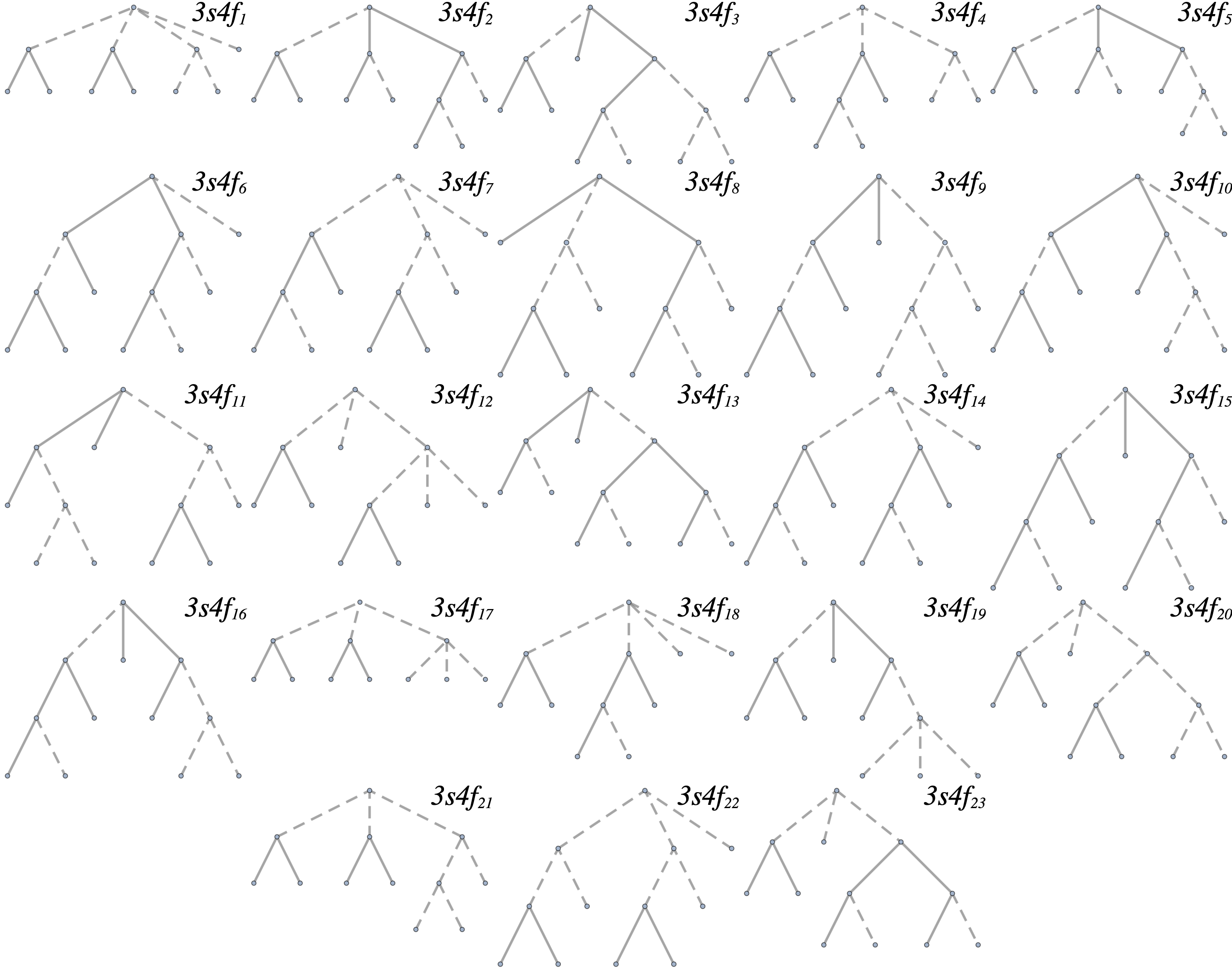
(a)

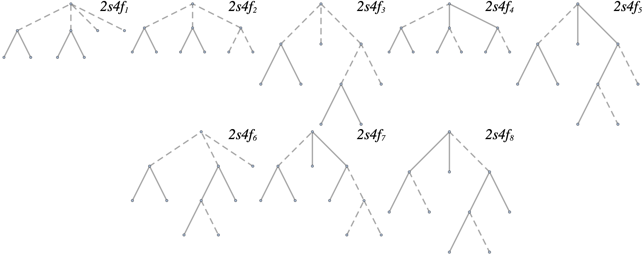
(b)

Figure 9: (a) The figure shows the tree-level topologies relevant to $3s4f$ operators. Topologies $3s4f_{3}$, $3s4f_{13}$, $3s4f_{20}$ and $3s4f_{23}$ imply one exotic field that couples only to other exotics in the diagram. This topology class is relevant to a large number of dimension-nine operators, and these are the lowest-dimensional examples of operators containing this property in our listing. (b) The two-scalar–four-fermion topologies associated with dimension-nine single-derivative operators in our catalogue. Since only single-derivative operators furnish these graphs, only those topologies containing at least one arrow-preserving internal fermion line are relevant. These are topologies $2s4f_{4}$ – $2s4f_{8}$; the other fermion propagator in $2s4f_{4}$ and $2s4f_{5}$ must be arrow violating. Topologies $2s4f_{1}$ – $2s4f_{3}$ each give rise to completions involving exotic Proca fields.

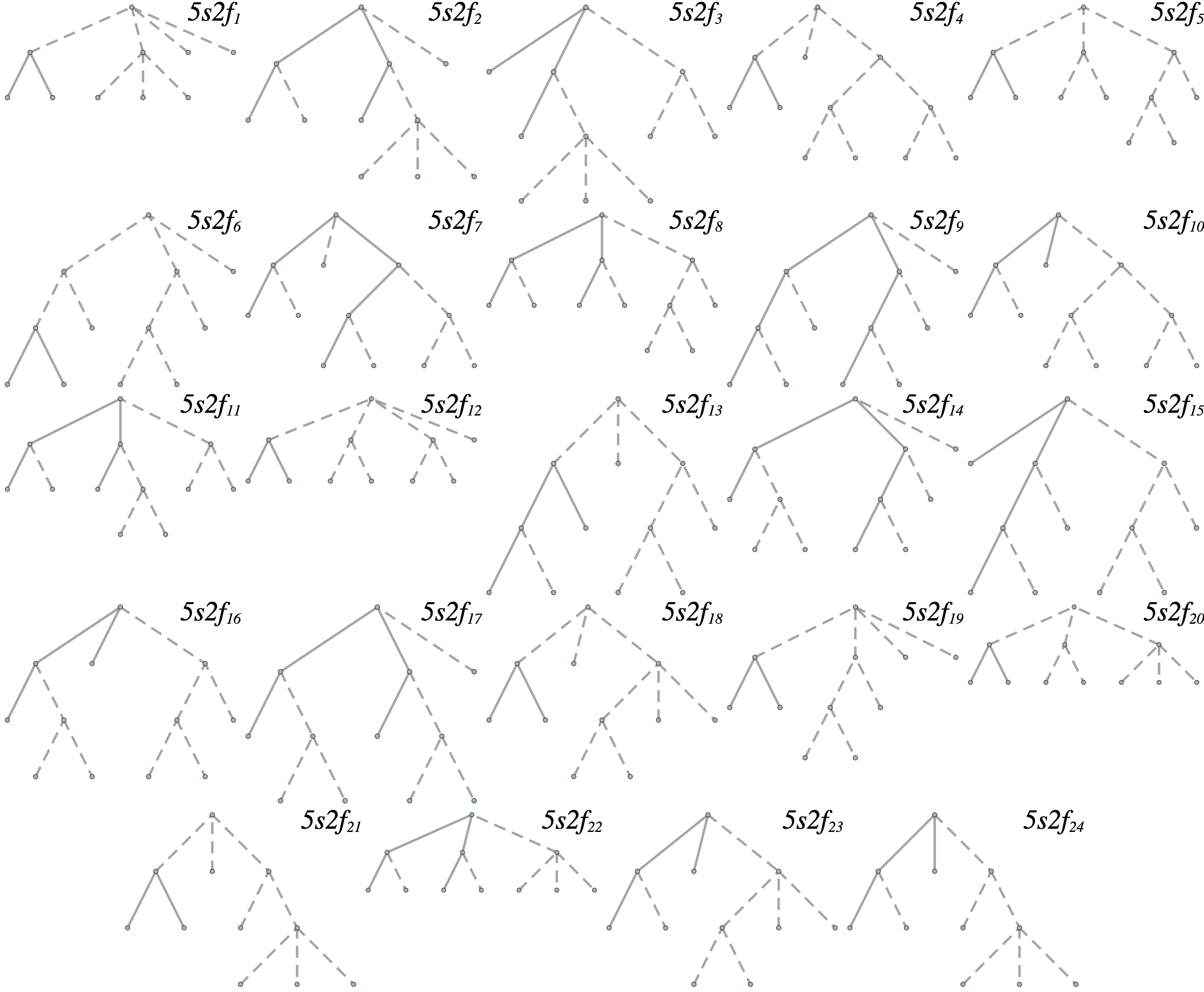
(a)

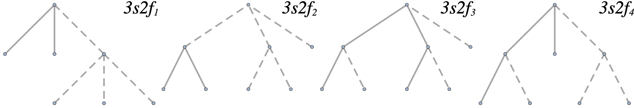
(b)

Figure 10: (a) The $5s2f$ topologies relevant only to the single-derivative operator $\mathcal{O}_{D20}$. Only those topologies allowing one arrow-preserving internal fermion line give completions allowed in our framework. Topologies $5s2f_{4}$, $5s2f_{7}$ and $5s2f_{10}$ contain heavy fields that couple only to other exotics in the diagram. (b) The UV diagrams associated with the $3s2f$ operator $\mathcal{O}_{D21}$. Only the last two diagrams can generate the operator under our model-building assumptions.

Dimension eleven

By far the largest class of operators at dimension eleven is the $2s6f$ topology type, for which the topologies are presented in Fig. 11. These operators are mostly formed as products of $0s6f$ dimension-nine operators with $H^{\dagger}H$, or $1s4f$ dimension-seven operators with SM Yukawa couplings. They are operators $\mathcal{O}_{21}$ through to $\mathcal{O}_{65}$, excluding the structures associated with $\mathcal{O}_{61}$, as well as $\mathcal{O}_{75}$, $\mathcal{O}_{76}^{\prime}$ and $\mathcal{O}_{82}$. The only other major class relevant to the derivative-free dimension-eleven operators is $5s4f$ for which there are 264 tree-level topologies. These are presented with our example code, along with the topologies relevant to the single $6s2f$ operator $\mathcal{O}_{1}^{\prime\prime\prime}$. This dimension-eleven generalisation of the Weinberg operator has already received some attention in the literature Anamiati:2018cuq .

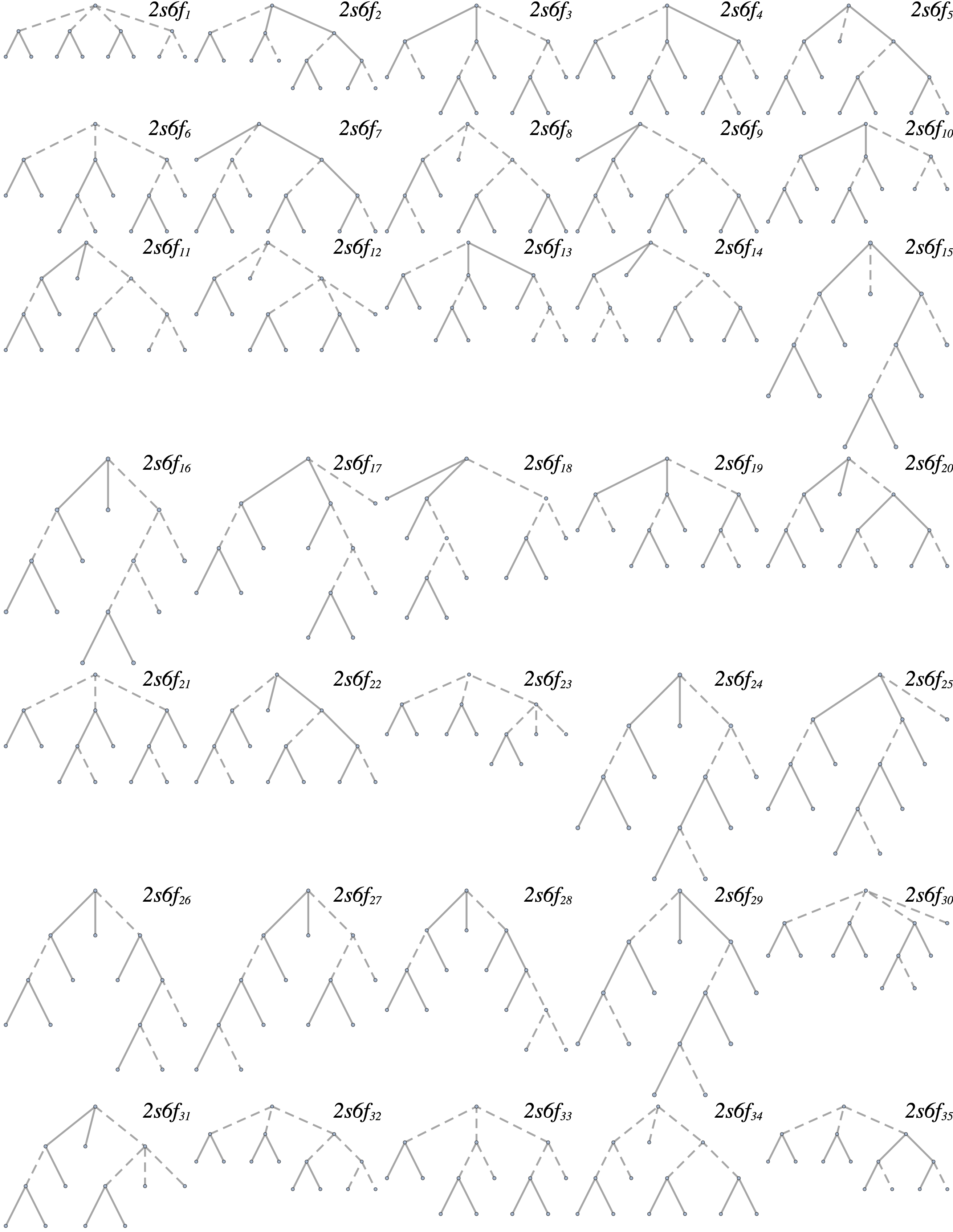
Figure 11: The tree-level topologies associated with the large class of $2s6f$ dimension-eleven operators in our listing. A number of graphs display the feature — less common at dimension nine — that an exotic field in the diagram couples only to other internal lines.

4.2.2 Model filtering

The completions constructed by exploding the $\Delta L=2$ operators are not all automatically guaranteed to provide the leading-order contribution to the neutrino mass. The same $\Delta L=2$ Lagrangian may, for example, inevitably imply another, larger contribution. Alternatively, the dominant contribution may come from other LNV combinations of couplings in the model’s full Lagrangian. The relative importance of different mechanisms may also depend on the assumptions of the model builder. Some neutrino-mass diagrams will dominate over others only in certain regions of parameter space. Are these regions accessible without large hierarchies in exotic couplings? Are such hierarchies acceptable, if necessary to render a mechanism dominant? What about exotic flavours or additional symmetries? Model filtering is the process of removing those models that, under some set of assumptions, do not provide the leading-order contribution to the neutrino mass. Our approach to filtering neutrino mass models is contrasted against other possible approaches below, and we also make more general comments about model filtering in other contexts. We mention that the following discussion of filtering is similar in intent to that of ‘genuineness’ in the loop-level matching paradigm Bonnet:2012kz ; Sierra:2014rxa ; Cepedello:2018rfh ; Farzan:2012ev . We sometimes adopt this notation as well, and call models ‘genuine’ if they represent the dominant contribution to the neutrino mass.

Filtering criterion

We begin by noting that model filtering is ubiquitous when considering tree-level effects. Here, the filtering criterion is unambiguously the operator dimension, since higher-dimensional operators are inevitably suppressed compared to lower-dimensional ones. With regard to the $\Delta L=2$ EFT, such a dimension-focused criterion is useful for thinking about LNV scattering events, for example. As discussed in Sec. 4.1, the operator dimension is also a rough indication of the predicted neutrino-mass scale, and therefore has some utility in anticipating which models will dominate the neutrino mass.

We point out that this approach to model filtering allows for the immediate rejection of some models, already during the process of opening up the operator. This can happen, for example, when a contraction introduces an exotic particle transforming like a SM field. Taking $\mathcal{O}_{2}$ as an example, contractions like

$$\overset{\tiny\varphi^{\dagger}\sim(\mathbf{1},\mathbf{2},\tfrac{1}{2})}{\wick{L^{i}\c{L}^{j}L^{k}\c{\bar{e}}H^{l}}\epsilon_{ij}\epsilon_{kl}}\rightarrow L^{i}L^{k}\tilde{\varphi}^{j}H^{l}\epsilon_{ij}\epsilon_{kl},$$ (56)

with $\tilde{\varphi}$ a second Higgs doublet, always imply that further contractions will produce seesaw fields, since the RHS of Eq. (56) has the same structure as the Weinberg operator. We note that for fermions the situation is more subtle because of the Lorentz structure. Specifically, although $H\bar{u}$ transforms like $Q^{\dagger}$ under $G_{\text{SM}}$, the Lorentz transformation properties are different. The derivative contraction $(D^{\alpha\dot{\alpha}}H)\bar{u}_{\alpha}$ does transform like $Q$ under $\mathrm{SU}(2)_{+}\otimes\mathrm{SU}(2)_{-}\otimes G_{\text{SM}}$ and that makes a number of such contractions forbidden if one is interested in only dominant contributions according to the mass-dimension criterion. This is the same phenomenon as that seen in the paradigmatic opening of the derivative operator $\mathcal{O}_{D3}$ given in Sec. 3.2.2, where an exotic field transforming like $L$ [see Eq. (44)] lead to a similar Weinberg-like operator at an intermediate stage in the completion procedure. We note that this does not completely rule out exotic copies of SM fields featuring in radiative neutrino mass models. Using $\mathcal{O}_{2}$ again as an example:

$$\overset{\tiny\varphi^{\dagger}\sim(\mathbf{1},\mathbf{2},\tfrac{1}{2})}{\wick{L^{i}L^{j}\c{L}^{k}\c{\bar{e}}H^{l}}\epsilon_{ij}\epsilon_{kl}}\rightarrow L^{i}L^{j}\tilde{\varphi}^{k}H^{l}\epsilon_{ij}\epsilon_{kl}$$ (57)

is allowed, since the $\mathrm{SU}(2)_{L}$ structure of this operator differs to that of the Weinberg operator. Similarly, vector-like quarks and leptons are extensively found in completions of both derivative and non-derivative operators after the filtering procedure, but their SM and Lorentz quantum numbers are interchanged with respect to their SM counterparts. For example, a particular completion of $\mathcal{O}_{3a}$ is

$$\overset{\tiny U\sim(\mathbf{3},\mathbf{1},\tfrac{2}{3})}{\wick{L^{i}L^{j}\c{Q}^{k}\bar{d}\c{H}^{l}\epsilon_{ij}\epsilon_{kl}}}\rightarrow\overset{\tiny\mathcal{S}^{\dagger}_{1}\sim(\mathbf{1},\mathbf{1},-1)}{\wick{\c{L}^{i}\c{L}^{j}U\bar{d}\epsilon_{ij}\epsilon_{kl}}}\rightarrow\mathcal{S}^{\dagger}_{1}U\bar{d}\ ,$$ (58)

which contains the vector-like quark $U+\bar{U}^{\dagger}$. Note however that $U$ transforms like $\bar{u}^{\dagger}$ under $G_{\text{SM}}$, but oppositely under the Lorentz group. It is true that $\bar{U}$, the vector-like partner of $U$, does transform like $\bar{u}$, but this plays no role in the operator.

Since we are most interested in radiative neutrino mass, a more direct and relevant filtering criterion in our case is the neutrino-mass estimate from the closure graph of the operator. This is the metric we use to compare and filter models in the results we present in Sec. 5. Whichever filtering criterion is chosen, the conditions for generating the lower-dimensional operator or the dominant neutrino self-energy graph still depend on the filtering philosophy.

Filtering philosophy

The filtering criterion defines a hierarchy among the effective operators. If one is interested in tree-level effects, then operators of low dimension have a high priority in the sense that their effects are dominant over those of high-dimensional operators, whose influence is suppressed by additional powers of $\Lambda$. Similarly, the operators whose closure graphs imply large contributions to the neutrino mass have a higher priority than those implying small contributions.

One could take the view that it is sufficient for a subset of the field content associated with a completion of a high-priority operator to be present in that of a lower-priority one for it to be filtered out, even if the relevant diagrams depend on entirely different couplings and interactions. We call this perspective democratic, in the sense that it treats all allowed couplings and interactions fairly and ignores possible hierarchies in free parameters. A democratic approach would then filter out all completions of $\Delta L=2$ operators of mass dimension larger than five containing one of the seesaw fields, for example, since these always imply a dominant contribution from the dimension-five Weinberg operator. Even if the same couplings are not present in both diagrams, there is no reason, on this view, for one coupling to be very much larger than another, making the tree-level contribution dominant.

An alternative approach might be to filter out only those completions that necessarily lead to subdominant contributions to the neutrino mass in all regions of parameter space. Naively it seems that neutrino-mass mechanisms involving different couplings would all survive the filtering process in this case, since the relative ordering of the contributions from each diagram depends on the chosen values of the coupling constants. This is in general only guaranteed if a symmetry is recovered in the Lagrangian when one coupling is turned off, so that the forbidden coupling is not generated at some higher order in perturbation theory. We call this approach stringent filtering, since the conditions for removing a model are more difficult to satisfy.

For our results in Sec. 5 we take an intermediate view, leaning more towards the democratic side. We filter on the basis of particle content, but always keep track of the baryon-number assignment of the field. We then keep models with identical SM quantum numbers if the baryon-number assignments of the fields differ. With a concrete example, we treat $\zeta^{(\prime)}\sim(\bar{\mathbf{3}},\mathbf{1},\tfrac{1}{3})$ in $x(L^{i}Q^{j})\zeta^{\{kl\}}\epsilon_{ik}\epsilon_{jl}$ and $y(Q^{i}Q^{j})\zeta^{\prime\{kl\}}\epsilon_{ik}\epsilon_{jl}$ as different fields.

In practice, we enumerate the completions of the operators in order of their estimated contribution to the neutrino mass. We associate a prime number with each exotic field encountered, including baryon-number as a distinguishing property. Models then correspond to products of prime numbers. As we explode each operator in order, we remove models from the list of completions if their characteristic number is divisible by that of any models already seen. In this way, we remove those mechanisms that are subdominant contributions to the neutrino mass in the democratic sense.

We emphasise that this procedure is not sufficient to fully ensure that the remaining models are genuinely dominant contributions to the neutrino mass. For example, it may be the case that the Weinberg operator is generated by loops of a subset of the exotic particles in one of our models. We are not sensitive to these models since we are concerned only with tree-level completions of the operators. One-loop contributions to the neutrino mass from heavy loops can be diagnosed easily on topological grounds. For example, topology T-3 of Ref. Bonnet:2009ej will come about whenever the neutrinos in the diagram are connected by a single exotic fermion Angel:2012ug . At two-loops, one could check the full gauge- and Lorentz-invariant Lagrangian for each model against Table 1 of Ref. Sierra:2014rxa , for example. We do not include this in our default filtering procedure, since it would require generating the full Lagrangian of each model. This is a computationally prohibitive task, especially since Table 4 suggests that the completions of some operators can contain up to six exotic fields. Should any model from our database be chosen for further study, the full Lagrangian can be generated with the functions in our example code and studied for the presence such heavy loops. We note that sometimes the presence of a heavy loop can be diagnosed from the neutrino self-energy graph, or even the tree-level topology, and we give a detailed example of such a case in Sec. 5.2.1. An additional filter on the models that goes beyond our initial tree-level filtering analysis is the possibility of exotic fields gaining vacuum expectation values. In this case, diagrams may exist that imply larger contributions to the neutrino mass than that suggested by our approach, and we are not sensitive to these since they generate exotic operators other than the Weinberg operator at the low scale. Examples are presented in Refs. Popov:2019tyc ; Babu:2020hun , where in both cases a two-loop completion of the Weinberg operator also generates the exotic operator $LLH^{\dagger}\Theta_{3}$, where $\Theta_{3}\sim(\mathbf{1},\mathbf{4},\tfrac{3}{2})_{S}$.

We note that our model database gargalionis_john_2020_4054618 contains both the unfiltered completions of the operators in Table LABEL:tab:long, as well as the models filtered according to the above method. Our example code also includes functions for filtering on interactions rather than fields, and finding $\mathrm{U}(1)$ symmetries present in models’ Lagrangians. Thus, the results presented in Sec. 5 and Table LABEL:tab:long can be readily reproduced with alternative filtering criteria, philosophies or approaches.

5 Models

In this section we present the radiative models derived by exploding the $\Delta L=2$ operators catalogued in Table LABEL:tab:long. We give an overview of the models, and explore their particle content and the effects of the partial model-filtering method we present in Sec. 4.2.2. We do not provide the entire listing of models here because there are very many, but instead give some examples. We point the interested reader to our database for the full searchable listing.

We distinguish the terms ‘model’ and ‘neutrino-mass mechanism’ or ‘$\Delta L=2$ Lagrangian’ in this section. By model we mean a collection of particle content. Those same multiplets may have many combinations of couplings that violate lepton-number by two units, leading to meany neutrino-mass mechanisms, or $\Delta L=2$ Lagrangians. We use the word ‘completion’ here to mean a neutrino-mass mechanism derived from a particular effective operator. Used in this way, the same $\Delta L=2$ Lagrangian may be shared by two completions, but they correspond to the same model. We also remind the reader that we use the words ‘field’ and ‘multiplet’ interchangeably.

We note here that the following analysis does not include the dimension-eleven generalisation of the Weinberg operator $\mathcal{O}_{1}^{\prime\prime\prime}$, since the operator has an unwieldy number of topologies and the relevant tree-level completions have already been studied in the literature Anamiati:2018cuq .

5.1 Overview

The models are generated by running the algorithm summarised in Sec. 3.3, as found in our example code, on our catalogue of the $\Delta L=2$ operators. The results for the number of completions before and after filtering are presented in Table LABEL:tab:long. In the language of Sec. 4.2.2, we use the democratic filtering procedure with the neutrino-mass scale as the filtering criterion for these data. We note again that this leaves us with an overestimate of the actual number of genuine neutrino-mass models. Even so, one can see that 54 operators end up with no completions after filtering, ruling them out as possibly playing a dominant role in generating the neutrino masses, at least according to our model-building assumptions. The complete list of unfiltered $\Delta L=2$ Lagrangians and tree-level completion diagrams is compiled in our database, and the documentation provides information for how to perform different kinds of filtering on the models.

The database contains 430,810 inequivalent $\Delta L=2$ Lagrangians before filtering. Counted democratically (i.e. by particle content) these correspond to 141,989 unfiltered models. Of the distinct Lagrangians, only around $3\%$ (11,483) survive democratic filtering with the neutrino-mass criterion. This corresponds to 11,216 distinct models. In our filtering analysis we also incorporate information from the one-loop study of the Weinberg operator done in Ref. Bonnet:2012kz . We generate a listing of the models from Tables 2 and 3 of Ref. Bonnet:2012kz with hypercharges that are multiples of $1/6$ in the range $[-3,3]$ and ranges for the $\mathrm{SU}(3)_{c}$ and $\mathrm{SU}(2)_{L}$ representations that cover those of the exotic fields featuring in our models. We remove the completions in our listing that contain a subset of these fields and imply neutrino masses suppressed by more than one loop factor, since the models presented in Ref. Bonnet:2012kz generate the Weinberg operator at one loop.

We visualise the number of models with democratic and no filtering in Fig. 12 broken down by mass dimension. After filtering there are three models at dimension five, 16 models at dimension seven, 244 models at dimension nine and 10,969 models at dimension eleven. It is clear that the number of filtered neutrino-mass models grows with operator dimension, which is perhaps unintuitive. For any high dimensional operator, there are competing effects influencing the number of viable completions. First, the large number of models derived already from lower-dimensional operators means that the chances some model will be filtered out are larger. Second, high dimensional operators involve more fields, meaning that there are more combinations of contractions that can be made, and therefore more completions expected. Despite the increased filtering odds, evidently the combinatorial explosion of different models wins.

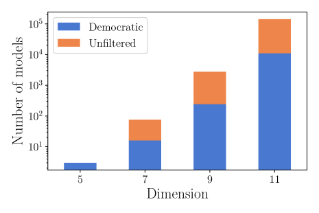
Figure 12: The bar chart shows the number of distinct Lagrangians derived from operators of different mass dimension. The orange bars show the number of distinct unfiltered models. The blue bars show the number after democratic filtering. The number of filtered completions grows with mass dimension.

In Fig. 13 we present data relevant to the number of fields present in the models. Fig. 13(a) shows the number of exotic scalars and fermions present in the completions. Despite the fact that the UV topologies associated with some derivative operators allow completions containing no scalars, we find that only the Weinberg-like operators keep their fermion-only models after the democratic filtering procedure. By far the most common kinds of models contain five heavy fields, especially three fermions and two scalars, or two fermions and three scalars. This is due to the fact that, as is clear from Fig. 12, most of the models generate dimension-eleven operators. In Fig. 13(b) we show the estimated new-physics scale $\Lambda$ against the number of fields featuring in the models. With the exception of one model with two fields, those required to lie at collider-accessible energies contain three or more fields. Models with few fields that imply suppressed neutrino masses, or equivalently a low new-physics scale, have a kind of selection pressure acting against them: since there are few fields, it is likely they will arise in the completion of other operators, that generally will filter out the former and imply a larger value of $\Lambda$. At dimension-seven, for example, $\mathcal{O}_{8}$ is generated by models featuring two fields and predicts that these should not be heavier than about $15\text{\,}\mathrm{TeV}$. However, of its four tree-level completions, only one survives the filtering procedure. This is the outlier two-field model evident in the figure. It was first derived in Ref. Cai:2014kra and later in Ref. Klein:2019iws . The model contains the fields $\Pi_{1}\sim(\mathbf{3},\mathbf{1},\tfrac{1}{6})_{S}$ and $Q_{7}\sim(\mathbf{3},\mathbf{2},\tfrac{7}{6})_{F}$. We list the models containing three exotic fields that are required to lie below $100\text{\,}\mathrm{TeV}$ in Sec. 5.2.

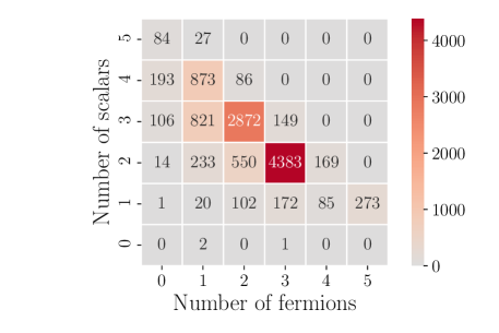
(a)

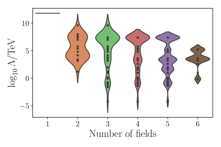
(b)

Figure 13: (a) The number of filtered models containing different numbers of exotic scalar and fermion fields. Most models contain five fields, with the most common combination being three fermions and two scalars. The fermion-only models are associated only with Weinberg-like operators. (b) The rough upper bound on the new-physics scale $\Lambda$ shown against the number of exotic fields introduced in the models. The black dots show the upper bound on the scale of the new physics for each model. A given black dot generally denotes more than one model. Each strip is a smoothed histogram of the number of models having a given $\Lambda$ as the new-physics upper bound for the specified number of fields. A sizeable class of models are testable at current or future collider experiments.

Of the unfiltered 430,810 models, close to $67\%$ (290,492) contain at least one of the seesaw fields: $N\sim(\mathbf{1},\mathbf{1},0)_{F}$, $\Xi_{1}\sim(\mathbf{1},\mathbf{3},1)_{S}$ or $\Sigma\sim(\mathbf{1},\mathbf{3},0)_{F}$. We present the exact breakdown by the interactions involved in the models in Table 5. These are by far the most common fields appearing in the list of unfiltered models. Since our default filtering philosophy in this analysis is democratic, all of these are absent from the filtered list of models, and they only appear in completions of the Weinberg operator and $\mathcal{O}_{D2}$.

Field	Interactions	$\Delta L=2$ Lagrangians	Models
$N\sim(\mathbf{1},\mathbf{1},0)_{F}$	$LHN$	51,245 (11.9%)	17,139 (17.1%)
	Other	12,433 (2.9%)
$\Sigma\sim(\mathbf{1},\mathbf{3},0)_{F}$	$LH\Sigma$	87,535 (20.3%)	31,629 (31.5%)
	Other	28,157 (6.5%)
$\Xi_{1}\sim(\mathbf{1},\mathbf{3},1)_{S}$	$LL\Xi_{1}$	59,791 (13.0%)	51,576 (51.4%)
	$HH\Xi_{1}^{\dagger}$	95,410 (22.1%)
	Both	10,323 (2.4%)
	Other	30,761 (7.1%)

Table 5: The table shows the number of unfiltered models in which the seesaw fields appear. The category ‘other’ includes interactions such as $L\varphi N$, where one of the SM fields in the interaction has been replaced with an exotic copy, as well as couplings involving other exotic fields whose quantum numbers are unrelated to those of SM fields.

The distinct exotic fields appearing in the completions number 171, although five fields are completely removed following filtering. These are $(\mathbf{\bar{6}},\mathbf{1},\tfrac{7}{6})_{S}^{1/3}$, $(\mathbf{\bar{6}},\mathbf{3},\tfrac{5}{3})_{S}^{1/3}$, $(\mathbf{1},\mathbf{3},3)^{0}_{S}$, $(\mathbf{1},\mathbf{5},2)^{0}_{F}$ and $(\mathbf{\bar{6}},\mathbf{1},\tfrac{5}{3})^{1/3}_{S}$, where the superscript represents the $B$ assignment of the field. There are 83 different scalar fields and 83 different fermion species. We distinguish three broad classes of scalars on the basis of their interaction with the SM fermions: leptoquarks, diquarks and dileptons. For exotic fermions we differentiate between those arising from contractions between the Higgs and a SM quark (vectorlike quarks), and the Higgs and a SM lepton (vectorlike leptons). The relative frequencies with which these field classes appear in the filtered completions are shown in Fig. 14 as pie charts. The wedges represent the number of Lagrangians in which the field couples as a leptoquark, diquark, dilepton, vectorlike quark or vectorlike lepton. We label fields coupling in all other ways as ‘other’ in the figure. The most represented family of scalars are leptoquarks, with the most common field being $\Pi_{7}\sim(\mathbf{3},\mathbf{2},\tfrac{7}{6})_{S}$, commonly called $R_{2}$ in the literature Dorsner:2016wpm . This leptoquark appears in simplified models of $R_{D^{(*)}}$ and the neutral-current flavour anomalies like $R_{K^{(*)}}$, see e.g. Refs. Sakaki:2013bfa ; Angelescu:2018tyl ; Becirevic:2018uab ; Popov:2019tyc ; Becirevic:2017jtw . It was recently shown to be able to reconcile the discrepant measurements in the anomalous magnetic moments of both the muon and the electron Bigaran:2020jil ; Dorsner:2020aaz . The second most common scalar appearing in our neutrino-mass models is $\zeta\sim(\mathbf{\bar{3}},\mathbf{3},\tfrac{1}{3})_{S}$, frequently referred to as $S_{3}$. This leptoquark is a popular explanation of the neutral-current $b\to s$ anomalies such as $R_{K^{(*)}}$, see e.g. Hiller:2014yaa ; Gripaios:2014tna ; Hiller:2017bzc ; Dorsner:2017ufx ; Angelescu:2018tyl . The most frequently encountered fermions are vectorlike quarks, with the most common being $T_{2}\sim(\mathbf{3},\mathbf{3},\tfrac{2}{3})_{F}$. It contains components that mix with both the up- and down-type SM quarks. We emphasise that the plots and numbers presented here are directly related to our filtering and model-counting conventions. In Fig. 14 for example, we do not count fields just by their quantum numbers, but also include coupling information as discussed above. Additionally, we count independent Lagrangians as different models rather than just counting distinct sets of fields, which is perhaps more in line with our ‘democratic’ approach to filtering. We note that the qualitative features discussed here are all relatively robust against these different conventions. We encourage the interested reader to explore our model database to see how different approaches to filtering and counting can answer specific questions they may have of the data.

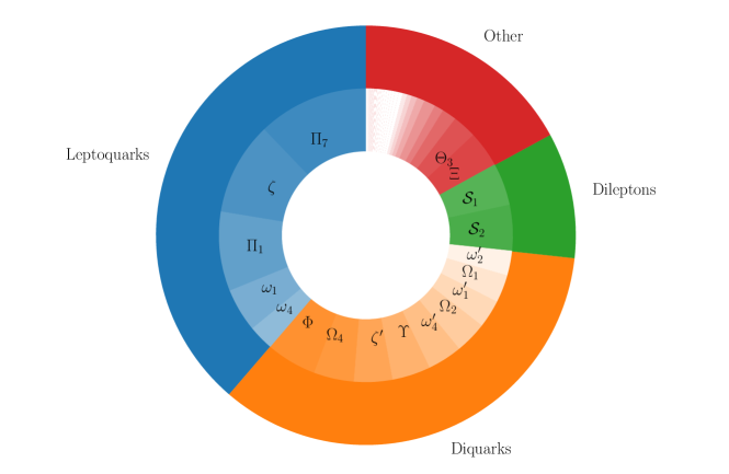
(a)

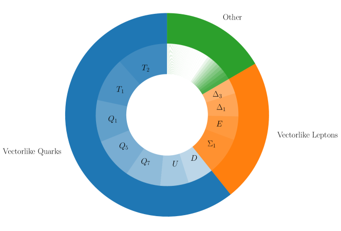
(b)

Figure 14: The number of models in which each field appears in the completions shown as a pie chart for scalars and fermions separately. The exotics are distinguished by their couplings to SM fields. (a) The pie chart of scalar fields appearing in the completions. Primed fields represent leptoquarks whose baryon-number assignment allows only the diquark couplings. (b) The pie chart of fermion fields appearing in the completions. See Table 2 or Ref. deBlas:2017xtg for the convention used for the field names.

We are also interested in the connectivity between fields as they feature in the models. To explore this we study a graph in which each vertex represents one of the 163 exotic fields introduced in the completions that contain at least two fields, and an edge is drawn between fields featuring together in a model. The graph is shown shown Fig. 15. The exterior sectors at each node represent the number of degree of the node. The edges in the graph are weighted by the number of times the corresponding pair of fields appears in the models; this is shown with a linear colour scaling in the figure. There are 3036 edges in the graph, and the average node degree is approximately 37. About a fifth of all possible connections in the graph are realised. The ten most heavily weighted edges, representing the ten most common pairs of fields appearing in the models, are shown in Table 6. Many of these correlations can be understood on the basis of common contractions in the derivation of the models, especially those involving $H$ or $L$. There is a propensity for scalars and fermions with the same gauge quantum numbers to appear in models together. This seems to come about from the fact that $H\otimes L$ is a gauge singlet but transforms like $(\mathbf{2},\mathbf{1})$ under $\mathrm{SU}(2)_{+}\otimes\mathrm{SU}(2)_{-}$. We note that all of the fields in the table have $|B|=\tfrac{1}{3}$, and so this edge cannot come about from $(\mathbf{\bar{3}},\mathbf{2},\tfrac{5}{6})_{F}\otimes\bar{d}\sim(\mathbf{3},\mathbf{2},\tfrac{7}{6})_{S}$.

Rank	Edge
1	$(\mathbf{3},\mathbf{3},\tfrac{2}{3})_{F}$, $(\mathbf{3},\mathbf{4},\tfrac{1}{6})_{S}$
2	$(\mathbf{3},\mathbf{2},\tfrac{1}{6})_{S}$, $(\mathbf{3},\mathbf{2},\tfrac{1}{6})_{F}$
3	$(\mathbf{3},\mathbf{3},\tfrac{2}{3})_{S}$, $(\mathbf{3},\mathbf{2},\tfrac{7}{6})_{S}$
4	$(\mathbf{3},\mathbf{2},\tfrac{7}{6})_{F}$, $(\mathbf{3},\mathbf{2},\tfrac{1}{6})_{S}$
5	$(\mathbf{3},\mathbf{3},\tfrac{2}{3})_{F}$, $(\mathbf{3},\mathbf{4},\tfrac{7}{6})_{F}$
6	$(\mathbf{\bar{3}},\mathbf{3},\tfrac{1}{3})_{S}$, $(\mathbf{3},\mathbf{4},\tfrac{1}{6})_{S}$
7	$(\mathbf{3},\mathbf{2},\tfrac{1}{6})_{F}$, $(\mathbf{3},\mathbf{3},\tfrac{2}{3})_{S}$
8	$(\mathbf{\bar{3}},\mathbf{3},\tfrac{4}{3})_{F}$, $(\mathbf{\bar{3}},\mathbf{2},\tfrac{5}{6})_{F}$
9	$(\mathbf{3},\mathbf{2},\tfrac{1}{6})_{S}$, $(\mathbf{3},\mathbf{3},\tfrac{2}{3})_{S}$
10	$(\mathbf{3},\mathbf{2},\tfrac{7}{6})_{S}$, $(\mathbf{\bar{3}},\mathbf{2},\tfrac{5}{6})_{F}$

Table 6: The table shows the pairs of fields that most often appear together in the filtered completions of the $\Delta L=2$ operators we consider. In the context of the graph of field connections introduced in the main text, these are the top ten edges by edge weight. Many of the connections can be understood on the basis of common couplings to SM fields, especially $L$ and $H$. For example, $(\mathbf{3},\mathbf{3},\tfrac{2}{3})_{F}\otimes L\sim(\mathbf{3},\mathbf{4},\tfrac{1}{6})_{S}$ and $(\mathbf{3},\mathbf{3},\tfrac{2}{3})_{S}\otimes H\sim(\mathbf{3},\mathbf{2},\tfrac{7}{6})_{S}$. All of the fields in the table have $|B|=\tfrac{1}{3}$.

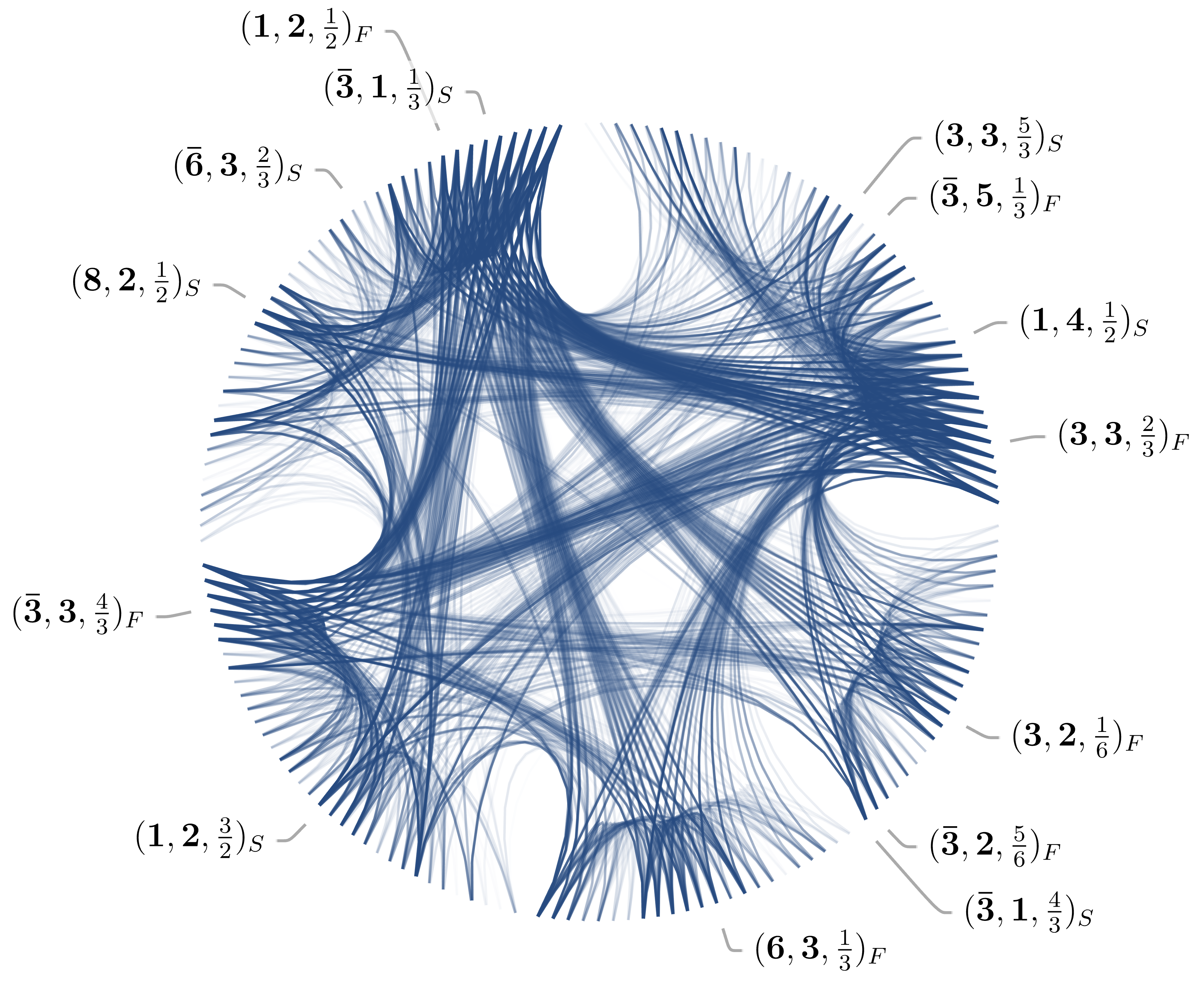
Figure 15: The graph is a representation of the connectivity between exotic fields in the neutrino-mass models. Each node represents an exotic field and edges connect fields featuring together in a neutrino-mass model. The colour is an indication of the weight of the edge, i.e. the number of times the two nodes appear in models together. The graph is clustered into roughly five communities within which there are many mutual connections. Only a handful of node labels are shown.

5.2 Example models

In this section we present some example neutrino-mass models, illustrating use cases of the model database, aspects to be careful of in its use, and representative features of the novel models derived from dimension-eleven and dimension-nine operators.

5.2.1 Simple models at the TeV scale

We are particularly interested in models that are simple, in the sense that they involve few exotic fields, and testable, in that they predict new physics at currently or nearly accessible energy ranges. We query our model database to return models featuring three fields or fewer with the estimated upper bound on the new-physics scale required to be between $700\text{\,}\mathrm{GeV}$ and $100\text{\,}\mathrm{TeV}$. The results of the query are presented in Table 7. There are twelve models listed, only one of which has explicitly appeared before in the literature to our knowledge: the completion of $\mathcal{O}_{8}$ discussed in Sec. 5.1. It is interesting to note that the scalar leptoquark $\Pi_{1}\sim(\mathbf{3},\mathbf{2},\tfrac{1}{6})_{S}$ appears in almost every model listed in the table. This suggests that our general analysis of the frequency of fields appearing in the completions in Sec. 5.1 may look different if specific selection criteria are placed on the data. We have checked the full Lagrangians implied by the field content of each model and found that seven of the models listed in the table imply the generation of the Weinberg operator through heavy loops. We emphasise that these non-genuine completions are potentially interesting and new radiative models, although the neutrino self-energy diagram will look different to that implied by the closure of the tree-level graph from which the model was derived. This means that the bound on the implied new-physics scale is in general higher than that suggested by the closure of the original operator. In this class are all of the models for which the upper bound on the new-physics scale is larger than $15\text{\,}\mathrm{TeV}$. This means that there are only five models in our database with fewer than four fields for which the upper bound on $\Lambda$ is between $700\text{\,}\mathrm{GeV}$ and $100\text{\,}\mathrm{TeV}$, and they all predict new physics below $15\text{\,}\mathrm{TeV}$. In the following we present two example models from the table:

1. We look at one of the models—the one derived from $\mathcal{O}_{62b}$—that generates the Weinberg operator through a heavy loop. We intend this to be an example of how this phenomenon can appear and how it is easy to diagnose in some cases.

2. We present a brief study of the implications for neutrino mass implied by the model given in the last row.

Field content	Operators	$\Lambda~{}[]$	Dominant?
$(\mathbf{3},\mathbf{2},\tfrac{1}{6})_{S}$, $(\mathbf{3},\mathbf{2},\tfrac{7}{6})_{F}$	$8$, $D15$	15	Y
$(\mathbf{1},\mathbf{2},\tfrac{1}{2})_{F}$, $(\mathbf{1},\mathbf{1},1)_{S}$, $(\mathbf{1},\mathbf{2},\tfrac{3}{2})_{S}$	$62b$	16	N
$(\mathbf{\bar{3}},\mathbf{2},\tfrac{5}{6})_{S}$, $(\mathbf{3},\mathbf{2},\tfrac{1}{6})_{F}$, $(\mathbf{3},\mathbf{2},\tfrac{1}{6})_{S}$	$8^{\prime}$	1	N
$(\mathbf{\bar{3}},\mathbf{1},\tfrac{1}{3})_{S}$, $(\mathbf{\bar{6}},\mathbf{2},\tfrac{1}{6})_{S}$, $(\mathbf{3},\mathbf{2},\tfrac{1}{6})_{F}$	$24f$	89	N
$(\mathbf{\bar{3}},\mathbf{3},\tfrac{1}{3})_{F}$, $(\mathbf{\bar{6}},\mathbf{2},\tfrac{1}{6})_{S}$, $(\mathbf{3},\mathbf{2},\tfrac{1}{6})_{S}$	$24d$	89	N
$(\mathbf{\bar{3}},\mathbf{2},\tfrac{5}{6})_{S}$, $(\mathbf{1},\mathbf{2},\tfrac{3}{2})_{F}$, $(\mathbf{3},\mathbf{2},\tfrac{1}{6})_{S}$	$8^{\prime}$	1	N
$(\mathbf{\bar{3}},\mathbf{3},\tfrac{1}{3})_{F}$, $(\mathbf{\bar{6}},\mathbf{4},\tfrac{1}{6})_{S}$, $(\mathbf{3},\mathbf{2},\tfrac{1}{6})_{S}$	$24f$	89	N
$(\mathbf{\bar{3}},\mathbf{1},\tfrac{1}{3})_{F}$, $(\mathbf{\bar{6}},\mathbf{2},\tfrac{1}{6})_{S}$, $(\mathbf{3},\mathbf{2},\tfrac{1}{6})_{S}$	$24d$	89	N
$(\mathbf{\bar{6}},\mathbf{2},\tfrac{7}{6})_{F}$, $(\mathbf{8},\mathbf{2},\tfrac{1}{2})_{S}$, $(\mathbf{3},\mathbf{2},\tfrac{1}{6})_{S}$	$20$	0.8	Y
$(\mathbf{6},\mathbf{1},\tfrac{4}{3})_{S}$, $(\mathbf{6},\mathbf{1},\tfrac{1}{3})_{F}$, $(\mathbf{3},\mathbf{2},\tfrac{1}{6})_{S}$	$20$	0.8	Y
$(\mathbf{6},\mathbf{2},\tfrac{5}{6})_{S}$, $(\mathbf{3},\mathbf{2},\tfrac{1}{6})_{F}$, $(\mathbf{3},\mathbf{2},\tfrac{1}{6})_{S}$	$50a,b$	10	Y
$(\mathbf{\bar{6}},\mathbf{2},\tfrac{1}{6})_{S}$, $(\mathbf{\bar{3}},\mathbf{2},\tfrac{5}{6})_{F}$, $(\mathbf{3},\mathbf{2},\tfrac{1}{6})_{S}$	$50a,b$	10	Y

Table 7: The table shows the models in our filtered list that contain fewer than four fields with the estimate of the upper-bound on the new-physics scale $\Lambda$ in the range $$700\text{\,}\mathrm{GeV}$<\Lambda<$100\text{\,}\mathrm{TeV}$$. Models containing colour sextet fields can be replaced with the corresponding colour-triplet fields with a different baryon-number assignment. The fields and models are listed in no special order. The scalar leptoquark $\Pi_{1}\sim(\mathbf{3},\mathbf{2},\tfrac{1}{6})$ appears in almost all of the models listed. Completions marked as non-dominant may be viable and interesting neutrino-mass models, but the main contribution to the neutrino mass does not come from the closure of the tree-level diagram from which the particle content was derived. This means, among other things, that the upper bound on the scale of the new physics associated with the model will differ to that presented here.

Model derived from $\mathcal{O}_{62b}$

The model derived from $\mathcal{O}_{62b}$ is especially simple since it does not require the imposition of $\mathrm{U}(1)_{B}$. The exotic fields introduced are $\Delta_{1}\sim(\mathbf{1},\mathbf{2},\tfrac{1}{2})_{F}$, $\mathcal{S}_{1}\sim(\mathbf{1},\mathbf{1},1)_{S}$ and $\chi\sim(\mathbf{1},\mathbf{2},\tfrac{3}{2})_{S}$. The additional interaction Lagrangian necessary to generate $\mathcal{O}_{62b}$ at tree level is $\Delta\mathscr{L}=\mathscr{L}_{Y}-\mathcal{V}$, with

$$-\mathscr{L}_{Y} =m_{\Delta_{1}}\bar{\Delta}_{1}\Delta_{1}+x_{[rs]}L^{i}_{r}L^{j}_{s}\mathcal{S}_{1}\epsilon_{ij}+y_{r}\bar{e}_{r}\bar{\Delta}_{1}^{i}\tilde{H}^{j}\epsilon_{ij}+z_{r}\bar{e}_{r}\tilde{\chi}^{i}\Delta_{1}^{j}\epsilon_{ij}\ ,$$ (59)

$$\mathcal{V} =m_{\mathcal{S}_{1}}^{2}\mathcal{S}_{1}^{\dagger}\mathcal{S}_{1}+m_{\chi}^{2}\chi^{\dagger}\chi+wH^{i}\chi^{j}\mathcal{S}^{\dagger}_{1}\mathcal{S}^{\dagger}_{1}\epsilon_{ij}\ .$$ (60)

This implies that the neutrino-mass mechanism depends on 13 new parameters: nine Yukawa couplings, $w$ and the three masses; although there are a much larger number of terms present in the full Lagrangian of the model. Importantly, one of these is $x^{\prime}_{r}L_{r}^{i}\bar{\Delta}^{j}_{1}\mathcal{S}_{1}\epsilon_{ij}$, which we now show is sufficient to generate the Weinberg operator through a two-loop diagram containing one heavy loop.

The tree-level completion diagram and the neutrino-mass diagram relevant to the model are shown in Fig. 16. There are two- and three-loop neutrino self-energies, where the three-loop models arise by connecting the $H$ and $H^{\dagger}$ lines in Fig. 16(b) in all possible ways. In this case, the first part of the fermion line (highlighted in Fig. 16(b)) can be replaced with the aforementioned $L\bar{\Delta}_{1}\mathcal{S}_{1}$ vertex so that the left loop contains only $\mathcal{S}_{1}$, $\chi$ and the Dirac fermion $\Delta_{1}+\bar{\Delta}_{1}^{\dagger}$. (It can also be noticed from the tree-level opening in Fig. 16(a) that the $\Delta_{1}$ line can be connected directly to one of the $LL\mathcal{S}_{1}$ vertices, giving rise to a loop-level completion of $\mathcal{O}_{2}$.) This heavy-loop neutrino-mass diagram, although interesting in its own right, predicts a different mass-scale for the exotic fields (roughly ${10}^{6}\text{\,}\mathrm{TeV}$), and a different structure for the neutrino-mass matrix.

(a)

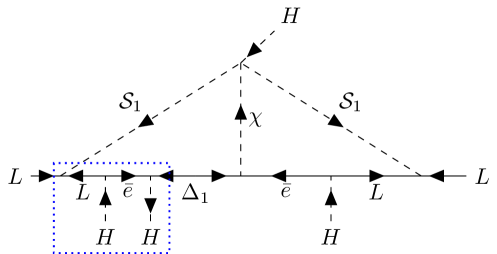
(b)

Figure 16: (a) The furnishing of the tree-level topology, labelled $2s6f_{4}$ in our scheme, that generates $\mathcal{O}_{62b}$ at tree level. The interactions allowed in the theory are such that the $\Delta_{1}$ line can be connected straight into one of the $LL\mathcal{S}_{1}$ vertices in place of an $L$, leading to a loop-level completion of $\mathcal{O}_{2}$. (b) The neutrino self-energy diagram relevant to the non-genuine completion of $\mathcal{O}_{62b}$. It is clear that this diagram does not represent the dominant contribution to the neutrino mass, since the the highlighted collection of fields can be replaced with the interaction $\bar{\Delta}_{1}L\mathcal{S}_{1}$. This leads to a diagram with heavy loop involving $\Delta_{1}$, $\chi$ and $\mathcal{S}_{1}$, which dominates the neutrino masses. In both cases, the relevant topology is CLBZ-7 in the classification of Ref. Sierra:2014rxa .

A genuine low-scale model

Below we present a brief exploration of the model derived from $\mathcal{O}_{50}$ that contains the exotic fields $\phi\sim(\mathbf{6},\mathbf{2},-\tfrac{1}{6})_{F}$, $\Pi_{1}\sim(\mathbf{3},\mathbf{2},\tfrac{1}{6})_{S}$ and $Q_{5}\sim(\mathbf{3},\mathbf{2},-\tfrac{5}{6})_{F}$. The estimate for the neutrino mass derived from the operator closure suggests this model’s exotic particle content should live roughly below $10\text{\,}\mathrm{TeV}$. The corresponding $\Delta L=2$ Lagrangian we write again as $\Delta\mathscr{L}=\mathscr{L}_{Y}-\mathcal{V}$, with

$$-\mathscr{L}_{Y} =x_{rs}L^{i}_{r}\bar{d}_{sa}\Pi_{1}^{aj}\epsilon_{ij}+y_{r}\phi^{\{ab\}i}\bar{u}_{ra}\bar{Q}^{j}_{5b}\epsilon_{ij}+z_{r}\bar{d}_{ra}H^{i}Q^{aj}_{5}\epsilon_{ij}+\text{h.c.}$$ (61)

$$\mathcal{V} =\lambda\tilde{\Pi}_{1a}^{i}\tilde{\Pi}_{1b}^{j}\phi^{\{ab\}k}H^{l}(\epsilon_{ik}\epsilon_{jl}+\epsilon_{il}\epsilon_{jk})\ .$$ (62)

We note that $\mathrm{U}(1)_{B}$ must be imposed on the Lagrangian to prevent terms like $\Pi^{3}_{1}H^{\dagger}$, $|\phi|^{2}\phi^{\dagger}\Pi_{1}$ and $|\Pi_{1}|^{2}\Pi_{1}\phi$ that destabilise the proton in the presence of the Yukawa interactions of Eq. (61). The field $\phi$ only couples to SM fermions together with $Q_{5}$ in this model, and so it generates no dimension-six operators at tree level. The completion graph and one of the neutrino self-energy diagrams are shown in Fig. 17. The tree-level topology is again $2s6f_{4}$, and the neutrino masses are realised at three and four loops, with the additional loop arising from the connection of an $H$ and $H^{\dagger}$. One of the loops involves a $W$ boson, and so the diagram does not fit into existing topological classifications. The three-loop diagram is similar to the topology $D_{9}^{M}$ of Ref. Cepedello:2018rfh , with one of the scalar lines replaced with a vector boson. The $W$ boson line must connect to $Q$ in the diagram, but could end on any field with non-trivial $\mathrm{SU}(2)_{L}$ charge. The connection to the $L$ line is shown, since the loop integral then depends on leptonic flavour indices, which can change the structure of the neutrino-mass matrix. There are also several ways of connecting the Higgs lines and only one combination is shown in the figure. The four-loop diagrams will be the dominant contribution to the neutrino masses for exotic fields above $4\pi v\approx$2\text{\,}\mathrm{TeV}$$.

The neutrino-mass matrix in this model can be estimated as

$$[\mathbf{m}_{\nu}]_{rs}=\frac{\lambda g^{2}}{(16\pi^{2})^{3}}\left(\frac{v^{2}}{\Lambda^{2}}+\frac{1}{16\pi^{2}}\right)\frac{1}{\Lambda}\sum_{t,u,v}x_{rt}z^{*}_{t}y^{*}_{u}[\mathbf{m}_{u}]_{u}V_{uv}[\mathbf{m}_{d}]_{v}x_{sv}I_{rstuv}+(r\leftrightarrow s)\ ,$$ (63)

where the $V_{rs}$ are CKM matrix elements, $\Lambda$ is the generic UV scale, and $I_{rstuv}$ is the loop function. The dependence on the masses of the up- and down-type quarks implies that the largest contributions to the neutrino masses will come from loops containing top and bottom quarks. If the parameters $y_{1,2}$, $x_{r1}$ and $x_{r2}$ play no significant role in the physics of neutrino mass, then the matrix will have rank 1 if the loop function carries no leptonic flavour indices. It may be the case that an additional generation of $Q_{5}$, $\phi$ or $\Pi_{7}$ is therefore required for the model to successfully reproduce the measured pattern of neutrino masses and mixings.

(a)

(b)

Figure 17: (a) The tree-level completion diagram for the model derived from exploding $\mathcal{O}_{50}$ and discussed in the main text. The topology is $2s6f_{4}$ in our classification scheme. The closure involves an arrow-preserving loop connecting the $\bar{d}^{\dagger}$ to one of the $\bar{d}$ lines, and the $W$-boson closure motif discussed in Sec. 4.1. (b) One of the neutrino-mass diagrams relevant to the model derived from $\mathcal{O}_{50}$. There is a three-loop diagram with the $H$ line broken into an $H^{\dagger},H$ pair that generates the dimension-seven generalised Weinberg operator. The four-loop diagrams all involve connecting the $H^{\dagger}$ to each of the three $H$ legs in the diagram. There are also multiple places the $W$ could end in the diagram, although it must couple to the $Q$ line. The four-loop diagrams will give larger contributions to the neutrino mass than the three-loop diagrams for $\Lambda\gtrsim$2\text{\,}\mathrm{TeV}$$.

5.2.2 A model derived from a derivative operator

We move on to discuss a model generating the single-derivative dimension-nine operators $\mathcal{O}_{D10a,b,c}$. The estimated upper-bound on the exotic scale is close to $1.5\text{\times}{10}^{3}\text{\,}\mathrm{TeV}$ in this case. The model contains the fields $\rho\sim(\mathbf{1},\mathbf{2},\tfrac{3}{2})_{S}$, $Q_{5}\sim(\mathbf{3},\mathbf{2},\tfrac{5}{6})_{F}$ and $\Sigma_{1}\sim(\mathbf{1},\mathbf{3},1)_{F}$. Such two-fermion–one-scalar models are unique to completions of single-derivative operators at dimension nine.

The part of the Lagrangian relevant to lepton-number violation is

$$-\Delta\mathscr{L}=x_{r}L_{r}^{i}\Sigma_{1}^{\{jk\}}H^{\dagger}_{k}\epsilon_{ij}+y_{r}L_{r}^{i}\rho^{j}\bar{\Sigma}_{1}^{\{kl\}}\epsilon_{ik}\epsilon_{jl}+z_{r}\bar{d}_{ra}H^{i}Q^{aj}_{5}\epsilon_{ij}+w_{r}\bar{u}_{ra}\rho^{i}Q_{5}^{aj}\epsilon_{ij}+\text{h.c.}$$ (64)

The only additions to the scalar potential are the expected $|\rho|^{2}|H|^{2}$ and $|\rho|^{4}$ terms, and these play no role in the lepton-number violation. Notably, there are no Yukawa couplings involving $\bar{Q}_{5}$, and the field $\rho$ generates no dimension-six operators at tree-level, since the naively expected coupling $H^{i}H^{j}H^{k}\rho_{k}\epsilon_{ij}$ vanishes. The model also has the nice feature that no baryon-number violating interactions are present.

The tree-level completion diagram and one of the neutrino-mass diagrams are shown in Fig. 18. The completion diagram has topology $2s4f_{8}$, which requires one of the heavy fermions to have an arrow-preserving propagator. The neutrino-mass diagram shown is cocktail-like Gustafsson:2012vj , although there are also two-loop diagrams generating $\mathcal{O}_{1}^{\prime}$ at the low scale, as well as other diagrams with the $W$ and $H$ lines in different places. The topology of the neutrino self-energy diagram is similar to $D^{M}_{15}$ in Ref. Cepedello:2018rfh .

The flavour structure of the neutrino-mass matrix has the approximate form

$$[\mathbf{m}_{\nu}]_{rs}=\frac{g^{2}}{(16\pi^{2})^{3}}\frac{1}{\Lambda}\sum_{t,u}y_{r}x_{s}w^{*}_{t}z_{t}[\mathbf{m}_{d}]_{t}V_{ut}[\mathbf{m}_{u}]_{u}I_{rstu}+(r\leftrightarrow s)\ .$$ (65)

The dependence on the up- and down-type mass matrices, as in the example presented in Sec. 5.2.1, means that the couplings $w_{1,2}$ and $z_{1,2}$ will not play an important role in generating the observed pattern of neutrino masses and mixings. In this case the matrix has at least rank 2, even if the leptonic-flavour structure of the loop integrals $I_{rstu}$ is flat. Thus, the structure of the neutrino masses and mixing parameters emerges mostly from the six parameters $x_{r}$ and $y_{r}$.

(a)

(b)

Figure 18: (a) The tree-level completion diagram for the model that generates the single-derivative operators $\mathcal{O}_{D10,a,b,c}$ and discussed in the main text. The topology is $2s4f_{8}$ in our classification scheme. This class of topologies is only relevant to single-derivative operators, and contains an arrow-preserving fermion propagator, that of $Q_{5}$ in the diagram. The closure of the diagram involves a $W$-boson loop, similar to that required in Fig. 17. (b) One of the neutrino-mass diagrams relevant to the model generating $\mathcal{O}_{D10a,b,c}$. The diagram generates the Weinberg operator as drawn, but additional diagrams exist with the central $H$ line cut into an $H,H^{\dagger}$ pair that generate $\mathcal{O}^{\prime}_{1}$ instead. These diagrams will only be relevant for exotic masses less than about $2\text{\,}\mathrm{TeV}$. Additional three-loop diagrams exist in which the Higgs coming from the $\Sigma_{1}LH^{\dagger}$ interaction loops into any of the other external $H$ fields. The $W$ boson must connect to the $Q$ line, but could end on any other field with non-trivial $\mathrm{SU}(2)_{L}$ charge. The topology is cocktail-like Gustafsson:2012vj , and resembles $D^{M}_{15}$ in Ref. Cepedello:2018rfh .

5.2.3 A model of neutrino mass and the flavour anomalies

Here we present a model designed specifically to generate a particular set of dimension-six operators. The example is motivated by the recent flavour anomalies: deviations from the SM seen in charged- and neutral-current $B$-meson decays. Key examples are the lepton-flavour-universality (LFU) ratios Lees:2012xj ; Lees:2013uzd ; Huschle:2015rga ; Hirose:2016wfn ; Abdesselam:2016cgx ; Aaij:2017tyk ; Aaij:2017uff

$$R_{D^{(*)}}=\frac{\Gamma(B\to D^{(*)}\tau\nu)}{\Gamma(B\to D^{(*)}\ell\nu)}\quad\text{ with }\ell\in\{e,\mu\}\ ,$$ (66)

for which the combined significance of the deviation from the SM is $3.1\sigma$ Amhis:2019ckw , and

$$R_{K^{(*)}}=\frac{\Gamma(B\to K^{(*)}\mu\mu)}{\Gamma(B\to K^{(*)}ee)}\ ,$$ (67)

both measured to be about $2.5\sigma$ away from $R_{K^{(*)}}\approx 1$ Aaij:2019wad ; Aaij:2017vbb . Along with the ratios $R_{K^{(*)}}$ sit a large class of discrepant measurements in $b\to s\ell\ell$ processes. These include differences from the SM expectation of angular observables in $B\to K^{*}\mu\mu$ Aaij:2015oid ; ATLAS-CONF-2017-023 ; CMS-PAS-BPH-15-008 ; Khachatryan:2015isa and suppressed branching ratios measured for $B\to K^{(*)}\mu\mu$ Aaij:2014pli and $B_{s}\to\phi\mu\mu$ Aaij:2015esa . The LFU ratios given in Eqs. (66) and (67) are theoretically very clean, since a large part of the theory uncertainty cancels in the ratio.

In the following we adhere to the conventions of Ref. Aebischer:2017ugx relevant to the Warsaw basis for the SMEFT and the flavio basis Straub:2018kue for the Weak Effective Theory (WET). The leptoquarks $\omega_{1}\sim(\mathbf{\bar{3}},\mathbf{1},\tfrac{1}{3})_{S}$ and $\Pi_{7}\sim(\mathbf{3},\mathbf{2},\tfrac{7}{6})_{S}$ can provide an explanation of the anomalies in $R_{D^{(*)}}$ with contributions to the SMEFT operators

$$[C_{lequ}^{(1)}]_{3332}=\begin{cases}-4[C_{lequ}^{(3)}]_{3332}&\text{for }\omega_{1}\\ 4[C_{lequ}^{(3)}]_{3332}&\text{for }\Pi_{7}\\ \end{cases}\ ,$$ (68)

since they have Yukawa couplings to left- and right-handed SM fields. [We note that Eq. (68) holds at the high scale, and the relation between the operators is altered by running.] The Yukawa terms are

$$-\mathcal{L}_{\omega_{1}} =f_{rs}L_{r}Q_{s}\omega_{1}+g_{rs}\bar{e}^{\dagger}_{r}\bar{u}^{\dagger}_{s}\omega_{1}+\text{h.c.}$$ (69)

$$-\mathcal{L}_{\Pi_{7}} =x_{rs}L_{r}\bar{u}_{s}\Pi_{7}+y_{rs}\bar{e}^{\dagger}_{r}Q^{\dagger}_{s}\Pi_{7}+\text{h.c.}$$ (70)

and these imply

$$[C_{lequ}^{(1)}]_{3332}=\begin{cases}\dfrac{f_{33}g_{32}^{*}}{2m_{\omega_{1}}^{2}}&\text{for }\omega_{1}\\ \dfrac{x_{32}^{*}y_{33}}{2m_{\Pi_{7}}^{2}}&\text{for }\Pi_{7}\\ \end{cases}$$ (71)

at tree level. A satisfactory explanation of $R_{D^{(*)}}$ requires $\mathcal{O}(1)$ couplings, e.g. Cai:2017wry ; Popov:2019tyc , and for $\Pi_{7}$ fits are consistent with the operator coefficient being purely imaginary, e.g. Angelescu:2018tyl .

The $b\to s$ data can be explained by the tree-level exchange of the leptoquark $\zeta\sim(\mathbf{\bar{3}},\mathbf{3},\tfrac{1}{3})_{S}$, which generates

$$[C_{lq}^{(1)}]_{2223}=3[C_{lq}^{(3)}]_{2223}\ ,$$ (72)

relevant for the neutral-current anomalies. Fits are usually performed to four-fermion operators in the WET, defined below the electroweak scale. For the $b\to s\ell\ell$ data, a good fit is given for Aebischer:2019mlg

$$C_{9}^{bs\mu\mu}=-C_{10}^{bs\mu\mu}=\frac{1}{2}\left(V_{tb}V_{ts}^{*}\frac{e^{2}}{16\pi^{2}}\frac{4G_{F}}{\sqrt{2}}\right)^{-1}\left[C_{lq}^{(1)}+C_{lq}^{(3)}\right]_{2232}\approx-0.5\ .$$ (73)

It was pointed out in Ref. Aebischer:2019mlg that there exists a mild tension between the fit to $R_{K^{(*)}}$ and the other anomalous $b\to s$ data, which can be reconciled with an additional LFU contribution to $C_{9}^{bs\ell\ell}$ such that

$$C_{9}^{bs\mu\mu}\approx-0.44\quad\text{ and }\quad C_{9}^{bs\ell\ell}\approx-0.5\ ,$$ (74)

for $\ell\in\{e,\mu,\tau\}$. A potential source of this universal contribution to $C_{9}$ is new physics in four-quark operators like Aebischer:2019mlg

$$[\mathcal{O}_{qu}^{(1)}]_{2322}=(\bar{Q}_{2}\gamma_{\mu}Q_{3})(\bar{u}_{2}\gamma^{\mu}\bar{u}_{2})\ ,$$ (75)

which can be generated, for example, by $\Phi\sim(\mathbf{8},\mathbf{2},\tfrac{1}{2})_{S}$. The relevant Yukawa terms are

$$-\mathscr{L}_{\Phi}=w_{rs}Q_{r}^{ai}\bar{u}_{sb}\Phi^{bj}_{\ a}\epsilon_{ij}+\text{h.c.}$$ (76)

and a contribution of about the right size to $C_{9}^{bs\ell\ell}$ can be generated while avoiding dijet exclusion bounds from the LHC for $m_{\Phi}\sim$2\text{\,}\mathrm{TeV}$$ and $|w_{22}|,|w_{32}|\sim 1$ Aebischer:2019mlg .

We construct a UV model that contains $\zeta$ and $\Phi$ as well as one of $\omega_{1}$ or $\Pi_{7}$ in an attempt to incorporate this explanation into a model of neutrino mass. We emphasise that our goal here is not to present the most elegant or motivated model of neutrino mass and the flavour anomalies, but rather to show that our database can be used to motivate complex models with a specific structure.

We query the filtered model database for neutrino-mass models that contain the interactions $Q\bar{u}\Phi$, needed to generate $\mathcal{O}_{qu}^{(1)}$; $LQ\zeta$, needed to generate $C_{9}^{bs\mu\mu}=-C_{10}^{bs\mu\mu}$; and one of $\omega_{1}$ or $\Pi_{7}$, required to explain $R_{D^{(*)}}$. Our query returns a number of models, and we choose one to study briefly below. We note that none of the models involve the leptoquark $\omega_{1}$, and none feature the interaction $\bar{e}^{\dagger}Q^{\dagger}\Pi_{7}$, implying some freedom in the explanation of $R_{D^{(*)}}$ since the couplings $y_{rs}$ of Eqs. (70) and (71) will be unrelated to the neutrino mass.

The model contains the additional fields $\Phi$, $\zeta$, $\Pi_{7}$ and $\eta\sim(\mathbf{8},\mathbf{1},1)_{S}$, necessary for lepton-number violation. It generates $\mathcal{O}_{29b}$, which implies an upper bound on the new-physics scale of roughly ${10}^{7}\text{\,}\mathrm{TeV}$. The additional piece of the Lagrangian is $\Delta\mathscr{L}=\mathscr{L}_{Y}-\mathcal{V}$, with

$$-\mathscr{L}_{Y} =x_{rs}L^{i}_{r}\bar{u}_{sa}\Pi^{ja}_{7}\epsilon_{ij}+y_{rs}\bar{e}^{\dagger}_{r}Q_{sai}^{\dagger}\Pi^{ai}_{7}+z_{rs}L^{i}_{r}Q^{ja}_{s}\zeta_{a}^{\{kl\}}\epsilon_{ik}\epsilon_{jl}+w_{rs}Q^{ai}_{r}\bar{u}_{sb}\Phi^{bj}_{\ a}\epsilon_{ij}+\text{h.c.}$$ (77)

$$\mathcal{V} =\kappa H^{i}\Phi^{aj}_{\ b}\eta^{\dagger b}_{\ \ a}\epsilon_{ij}+\lambda H^{i}\eta^{a}_{\ b}\tilde{\Pi}^{j}_{7a}\tilde{\zeta}^{b\{kl\}}\epsilon_{ik}\epsilon_{jl}+\text{h.c.}+\cdots\ ,$$ (78)

where we have only shown the part of the scalar potential relevant to lepton-number violation in this model, since the full expression contains a large number of terms. The leptoquark $\zeta$ has a diquark coupling which we forbid by imposing $\mathrm{U}(1)_{B}$ on the Lagrangian, assigning baryon numbers of $-\tfrac{1}{3}$ and $\tfrac{1}{3}$ to $\zeta$ and $\Pi_{7}$, respectively. (All other exotic fields have $B=0$.) The model contains 33 free parameters, although not all of them are necessary to address the flavour anomalies and generate viable neutrino masses.

The tree-level completion diagram and the neutrino self-energy diagram are shown in Fig. 19. The neutrino mass arises at two loops, and the topology has the feature that no fermion propagators are arrow-violating. This implies that the neutrino masses are not proportional to any SM-fermion masses. This feature has been studied before in the context of a specific UV model in Ref. Gargalionis:2019drk . The phenomenon is particular to models derived from operators whose closures feature arrow-preserving loops, as discussed in Sec. 4.1. From a model-building perspective, one consequence is that the neutrino masses need not be dominated by Yukawa couplings to SM fermions of the third generation. Indeed, motivated by the pattern of operators required to explain the flavour anomalies, we adopt textures for the Yukawa couplings of Eq. (77) that imply dominance of the bottom-quark couplings for $\zeta$, but the charm-quark couplings for $\Pi_{7}$:

$$\mathbf{x}=\begin{pmatrix}0&x_{12}&0\\ 0&x_{22}&0\\ 0&x_{32}&0\\ \end{pmatrix},\quad\mathbf{z}=\begin{pmatrix}0&0&z_{13}\\ 0&z_{22}&z_{23}\\ 0&0&z_{33}\\ \end{pmatrix}\ ,$$ (79)

where the additional coupling $z_{22}$ is required to generate the relevant dimension-six operators $[\mathcal{O}_{lq}^{(1,3)}]_{2232}$. Interestingly, the minimal set of couplings $w_{rs}$ that gives viable neutrino masses while incorporating the key ingredients required to generate both $[\mathcal{O}_{lq}^{(1,3)}]_{2232}$ and $[\mathcal{O}_{lequ}^{(1,3)}]_{3332}$ is

$$\mathbf{w}=\begin{pmatrix}0&0&0\\ 0&w_{22}&0\\ 0&w_{32}&0\\ \end{pmatrix}\ ,$$ (80)

which is exactly the correct set required to also generate the operator given in Eq. (75). Thus, there is a natural connection in this model between the explanation of the charged- and neutral-current anomalies through the neutrino masses. With the exception of $y_{33}$, all of the couplings featuring in the explanation of the flavour anomalies also play a role in the generation of the neutrino masses. The structure of the neutrino-mass matrix is

_rs $$\simeq\frac{\lambda\kappa}{(16\pi^{2})^{2}}\frac{v^{2}}{\Lambda^{2}}\sum_{t,u}[z_{rt}w_{tu}x_{su}+(r\leftrightarrow s)]$$ (81)

$$=\frac{\lambda\kappa}{(16\pi^{2})^{2}}\frac{v^{2}}{\Lambda^{2}}[z_{r2}w_{22}x_{s2}+z_{r3}w_{32}x_{s2}+(r\leftrightarrow s)]\ .$$

The matrix is rank 2, and so implies an almost massless neutrino. Since there is no suppression of the neutrino-mass scale by SM Yukawa couplings, we distinguish the UV scales $\Lambda$ and $\kappa$ so that

$$\Lambda\simeq\max\left(m_{\zeta},m_{\Phi},m_{\eta},m_{\Pi_{7}}\right)$$ (82)

and consider the region of parameter space in which $\lambda\kappa\ll\Lambda$.

An explanation of the flavour anomalies in this picture can be achieved with $\mathcal{O}(1)$ couplings for $\Pi_{7}$ and $\Phi$ at a few , and $\zeta$ at tens of . We take $\eta$ slightly heavier at $\sim$50\text{\,}\mathrm{TeV}$$ to decouple its phenomenology and aid in suppressing the neutrino mass. This implies $\lambda\kappa\sim$0.05\text{\,}\mathrm{GeV}$$ for neutrino masses saturating the atmospheric bound. This choice is technically natural, since in the limit of vanishing $\lambda$ or $\kappa$ the Lagrangian regains $\mathrm{U}(1)_{L}$. We rewrite Eq. (81) as

$$[\mathbf{m}_{\nu}]_{rs}=m_{0}[x_{s2}(z_{r2}w_{22}+z_{r3}w_{32})+(r\leftrightarrow s)]\ ,$$ (83)

where $m_{0}\approx\lambda\kappa v^{2}(16\pi^{2})^{-2}m_{\eta}^{-2}$. This allows for the adoption of a Casas–Ibarra-like parametrisation of the vectors $x_{s2}$ and

$$\mathbf{Z}=\begin{pmatrix}z_{13}w_{32}\\ z_{22}w_{22}+z_{23}w_{32}\\ z_{33}w_{32}\end{pmatrix}\ ,$$ (84)

so that Cai:2014kra

$$x_{r2} =\frac{\xi}{\sqrt{2m_{0}}}\left(\sqrt{m_{2}}u_{2}^{*}+i\sqrt{m_{3}}u_{3}^{*}\right)\ ,$$ (85)

$$Z_{r} =\frac{1}{\xi\sqrt{2m_{0}}}\left(\sqrt{m_{2}}u_{2}^{*}-i\sqrt{m_{3}}u_{3}^{*}\right)\ ,$$ (86)

where the $u_{i}$ are the $i$th columns of the PMNS matrix; $m_{i}$ are the neutrino masses, fixed by the measured squared mass differences and the choice of normal ordering; and $\xi$ is a free complex parameter. We find, for example, that the choices $m_{\Phi}=$2\text{\,}\mathrm{TeV}$$, $m_{\Pi_{7}}=$1\text{\,}\mathrm{TeV}$$, $m_{\zeta}=$15\text{\,}\mathrm{TeV}$$, $m_{\eta}=$50\text{\,}\mathrm{TeV}$$, $\lambda\kappa=$0.05\text{\,}\mathrm{GeV}$$, $\xi=e^{3i/2}$, $z_{23}=1$, $w_{22}=-w_{32}=1$ and $y_{33}=2e^{2i}$ give approximately the right values to generate the pattern of dimension-six operators discussed and explain the flavour anomalies. This includes the additional lepton-flavour universal contribution to $C_{9}^{bs\ell\ell}$, discussed in Ref. Aebischer:2019mlg . Although a more detailed study of the phenomenological implications of the model is beyond the scope of this simple example, we have shown how a specific UV scenario can be embedded into a radiative model in a way consistent with the measured neutrino masses and mixing parameters.

(a)

(b)

Figure 19: (a) The figure shows the tree-level completion diagram for the model constructed to address the flavour anomalies and neutrino masses. The topology is labelled $2s6f_{2}$ in our scheme. The closure contains two arrow-preserving loops, which arise by looping the $\bar{u}$ into the $\bar{u}^{\dagger}$ and the $Q$ into the $Q^{\dagger}$. (b) The self-energy diagram for the same model. The diagram has a CLBZ-10 topology in the language of Ref. Sierra:2014rxa . The neutrino masses are not suppressed by SM-fermion masses on account of the arrow-preserving fermion lines. This feature raises the bound on the new-physics scale relevant to the model, but also allows couplings to the second generation of fermions to play a role in the physics of neutrino mass. This is beneficial in our case since many of these couplings are involved in generating the pattern of dimension-six operators that motivates this example, and so provides for a more intimate connection between the flavour anomalies and neutrino masses.

6 Conclusions

We have described a procedure for building UV-complete models from effective operators in a way amenable to automation. We have applied the algorithm, as found in our publicly available example code neutrinomass2020 , to the $\Delta L=2$ operators in the SMEFT up to and including dimension eleven, producing just over 11,000 minimal and predictive models of radiative Majorana neutrino mass. We share our complete listing of models, as well as the set reduced by model filtering, in our searchable model database gargalionis_john_2020_4054618 .

Our analysis includes new operators that have not appeared in previous catalogues, along with updated estimates for the upper bounds on the new-physics scales associated with these. We performed a preliminary study of the UV models, showing that the most represented exotic fields featuring in the completions are leptoquarks. We find that a number of simple models predict new physics that must live below $100\text{\,}\mathrm{TeV}$. Adding the additional requirements that the models contain fewer than four exotic fields and that the new-physics scale should be larger than $700\text{\,}\mathrm{GeV}$ gives at most five models fitting this description, all of which predict new fields below $15\text{\,}\mathrm{TeV}$. One of these models was studied briefly, along with a model derived from a derivative operator, and one that addresses the flavour anomalies.

Our model database is perhaps a good laboratory for experiments in automated phenomenological analysis. Now that the models have been written down and compiled into this computationally accessible format, our hope is that a large number of them can be ruled out in a systematic way through improved model filtering, neutrino oscillation data, or collider constraints. Our results also pave the way for more detailed studies of the models that are currently accessible to experiments. As each model is tested, we will either get very lucky and discover the origin of neutrino masses at low energies, or else falsify these scenarios and build a stronger circumstantial case for those that cannot be tested at collider experiments.

Appendix A Table of operators

Below we present the catalogue of $\Delta L=2$ operators we use in our study. The operators are listed and labelled in a way consistent with the previous catalogues Babu:2001ex ; deGouvea:2007qla , although we enforce that operators with the same field content carry the same numerical labels. This means that our listing may contain more $\mathrm{SU}(2)_{L}$ structures for any numbered family of operators. Product operators as presented in the table must be read with care. This is just a convenient shorthand to represent the field-content of an operator and illustrate that isospin indices are internally contracted. For example, by writing $\mathcal{O}_{5b}=\mathcal{O}_{1}Q^{i}\bar{d}\tilde{H}^{j}\epsilon_{ij}$, we do not mean to suggest that Lorentz indices must be contracted internally to $\mathcal{O}_{1}$ and the down-type Yukawa.

In each row we also provide information relevant to the number of completions. The number of unfiltered models (sets of field content) derived from the operator using our techniques is presented, along with the number that survive the democratic filtering procedure with the neutrino-mass filtering criterion. A sizeable number of operators end up with no completions that can play a dominant role in the physics of neutrino mass.

Other information relevant to the operators is also shown, including the number of loops required for the operator closure (the same as the number of loops appearing in the associated neutrino self-energy diagram) and the upper-bound on the scale of the new physics generating the operator at tree level, derived from the atmospheric lower bound on the mass of the heaviest neutrino. Operators for which a range is given for the number of loops are those that generate the dimension-seven or dimension-nine analogues of the Weinberg operator. The additional Higgs fields in these diagrams can always be closed off, adding more loops to the neutrino self-energy while reducing the overall scale suppression. The contribution with the highest number of loops will dominate for scales $\Lambda\gtrsim 4\pi v$.

We remind the reader that our analysis does not include the number of unfiltered completions of $\mathcal{O}_{1}^{\prime\prime\prime}$. In this case, the number of filtered models comes from Ref. Anamiati:2018cuq . Other operators featuring a ‘—’ are non-explosive, i.e. they do not support tree-level topologies containing only scalars and fermions.

Table 8: The table displays our listing of the $\Delta L=2$ operators along with the number of completions before and after our model-filtering procedure, the number of loops in the neutrino self-energy diagram, and the upper bound on the new-physics scale associated with each operator. See the main text of the appendix for more information.

Labels	Operator	Models	Filtered	Loops	$\Lambda~{}[\text{TeV}]$
$1$	$L^{i}L^{j}H^{k}H^{l}\cdot\epsilon_{ik}\epsilon_{jl}$	3	3	0	$605\,520\,000\,000.000$
$2$	$L^{i}L^{j}L^{k}\bar{e}H^{l}\cdot\epsilon_{ik}\epsilon_{jl}$	8	2	1	$39\,226\,496.247\,131\,0$
$3a$	$L^{i}L^{j}Q^{k}\bar{d}H^{l}\cdot\epsilon_{ij}\epsilon_{kl}$	9	2	2	$231\,157.260\,299\,850$
$3b$	$L^{i}L^{j}Q^{k}\bar{d}H^{l}\cdot\epsilon_{ik}\epsilon_{jl}$	14	5	1	$92\,116\,154.108\,431\,4$
$4a$	$L^{i}L^{j}\tilde{Q}^{k}\bar{u}^{\dagger}H^{l}\cdot\epsilon_{ik}\epsilon_{jl}$	5	0	1	$3\,807\,173\,871.715\,94$
$4b$	$L^{i}L^{j}\tilde{Q}^{k}\bar{u}^{\dagger}H^{l}\cdot\epsilon_{ij}\epsilon_{kl}$	4	2	2	$9\,553\,762.748\,660\,82$
$5a$	$L^{i}L^{j}Q^{k}\bar{d}H^{l}H^{m}\tilde{H}^{n}\cdot\epsilon_{il}\epsilon_{jn}\epsilon_{km}$	790	36	2	$583\,332.360\,427\,892$
$5b$	$\mathcal{O}_{1}\cdot Q^{i}\bar{d}\tilde{H}^{j}\cdot\epsilon_{ij}$	492	14	1,2	$583\,332.360\,436\,087$
$5c$	$\mathcal{O}_{3a}\cdot H^{i}\tilde{H}^{j}\cdot\epsilon_{ij}$	509	0	2,3	$1463.823\,717\,411\,27$
$5d$	$\mathcal{O}_{3b}\cdot H^{i}\tilde{H}^{j}\cdot\epsilon_{ij}$	799	16	1,2	$583\,332.360\,436\,087$
$6a$	$L^{i}L^{j}\tilde{Q}^{k}\bar{u}^{\dagger}H^{l}H^{m}\tilde{H}^{n}\cdot\epsilon_{il}\epsilon_{jn}\epsilon_{km}$	289	14	2	$24\,109\,210.188\,402\,6$
$6b$	$\mathcal{O}_{1}\cdot\tilde{Q}^{i}\bar{u}^{\dagger}\tilde{H}^{j}\cdot\epsilon_{ij}$	177	0	1,2	$24\,109\,210.188\,402\,7$
$6c$	$\mathcal{O}_{4a}\cdot H^{i}\tilde{H}^{j}\cdot\epsilon_{ij}$	262	0	1,2	$24\,109\,210.188\,402\,7$
$6d$	$\mathcal{O}_{4b}\cdot H^{i}\tilde{H}^{j}\cdot\epsilon_{ij}$	208	0	2,3	$60\,499.909\,449\,799\,1$
$7$	$L^{i}\bar{e}^{\dagger}Q^{j}\tilde{Q}^{k}H^{l}H^{m}H^{n}\cdot\epsilon_{il}\epsilon_{jm}\epsilon_{kn}$	240	15	2	$248\,404.689\,368\,816$
$8$	$L^{i}\bar{e}^{\dagger}\bar{u}^{\dagger}\bar{d}H^{j}\cdot\epsilon_{ij}$	5	1	2,3	$15.176\,616\,300\,330\,9$
$9$	$L^{i}L^{j}L^{k}L^{l}\bar{e}\bar{e}\cdot\epsilon_{ik}\epsilon_{jl}$	14	1	2	$2541.151\,419\,979\,84$
$10$	$L^{i}L^{j}L^{k}\bar{e}Q^{l}\bar{d}\cdot\epsilon_{ik}\epsilon_{jl}$	50	1	2	$5967.422\,997\,480\,72$
$11a$	$L^{i}L^{j}Q^{k}Q^{l}\bar{d}\bar{d}\cdot\epsilon_{ij}\epsilon_{kl}$	48	0	3	$35.165\,341\,876\,509\,2$
$11b$	$L^{i}L^{j}Q^{k}Q^{l}\bar{d}\bar{d}\cdot\epsilon_{ik}\epsilon_{jl}$	72	16	2	$14\,013.386\,589\,589\,6$
$12a$	$L^{i}L^{j}\tilde{Q}^{k}\tilde{Q}^{l}\bar{u}^{\dagger}\bar{u}^{\dagger}\cdot\epsilon_{ik}\epsilon_{jl}$	19	0	2	$23\,937\,397.426\,140\,4$
$12b$	$L^{i}L^{j}\tilde{Q}^{k}\tilde{Q}^{l}\bar{u}^{\dagger}\bar{u}^{\dagger}\cdot\epsilon_{ij}\epsilon_{kl}$	17	4	3	$60\,068.760\,591\,350\,4$
$13$	$L^{i}L^{j}L^{k}\bar{e}\tilde{Q}^{l}\bar{u}^{\dagger}\cdot\epsilon_{ik}\epsilon_{jl}$	12	0	2	$246\,634.449\,053\,772$
$14a$	$L^{i}L^{j}Q^{k}\tilde{Q}^{l}\bar{u}^{\dagger}\bar{d}\cdot\epsilon_{ij}\epsilon_{kl}$	29	1	3	$1453.388\,627\,412\,85$
$14b$	$L^{i}L^{j}Q^{k}\tilde{Q}^{l}\bar{u}^{\dagger}\bar{d}\cdot\epsilon_{ik}\epsilon_{jl}$	43	1	2	$579\,175.279\,238\,636$
$15$	$L^{i}L^{j}L^{k}\tilde{L}^{l}\bar{u}^{\dagger}\bar{d}\cdot\epsilon_{ik}\epsilon_{jl}$	12	1	3	$1453.388\,627\,412\,85$
$16$	$L^{i}L^{j}\bar{e}\bar{e}^{\dagger}\bar{u}^{\dagger}\bar{d}\cdot\epsilon_{ij}$	13	1	3	$1453.388\,627\,412\,85$
$17$	$L^{i}L^{j}\bar{u}^{\dagger}\bar{d}\bar{d}\bar{d}^{\dagger}\cdot\epsilon_{ij}$	18	12	3	$1453.388\,627\,412\,85$
$18$	$L^{i}L^{j}\bar{u}\bar{u}^{\dagger}\bar{u}^{\dagger}\bar{d}\cdot\epsilon_{ij}$	22	8	3	$1453.388\,627\,412\,85$
$19$	$L^{i}\bar{e}^{\dagger}Q^{j}\bar{u}^{\dagger}\bar{d}\bar{d}\cdot\epsilon_{ij}$	27	0	3,4	$0.221\,892\,467\,282\,772$
$20$	$L^{i}\bar{e}^{\dagger}\tilde{Q}^{j}\bar{u}^{\dagger}\bar{u}^{\dagger}\bar{d}\cdot\epsilon_{ij}$	27	3	3,4	$0.797\,031\,006\,138\,724$
$21a$	$L^{i}L^{j}L^{k}\bar{e}Q^{l}\bar{u}H^{m}H^{n}\cdot\epsilon_{il}\epsilon_{jm}\epsilon_{kn}$	3943	1	2,3	$1561.833\,955\,204\,21$
$21b$	$L^{i}L^{j}L^{k}\bar{e}Q^{l}\bar{u}H^{m}H^{n}\cdot\epsilon_{ik}\epsilon_{jm}\epsilon_{ln}$	4080	4	3	$1561.830\,894\,069\,01$
$22a$	$L^{i}L^{j}L^{k}\tilde{L}^{l}\bar{e}\bar{e}^{\dagger}H^{m}H^{n}\cdot\epsilon_{il}\epsilon_{jm}\epsilon_{kn}$	726	0	2	$24\,282\,256.151\,783\,0$
$22b$	$\mathcal{O}_{2}\cdot\tilde{L}^{i}\bar{e}^{\dagger}H^{j}\epsilon_{ij}$	931	0	2	$24\,282\,256.151\,783\,0$
$23a$	$L^{i}L^{j}L^{k}\bar{e}\tilde{Q}^{l}\bar{d}^{\dagger}H^{m}H^{n}\cdot\epsilon_{il}\epsilon_{jm}\epsilon_{kn}$	780	0	2,3	$37.914\,827\,868\,419\,3$
$23b$	$\mathcal{O}_{2}\cdot\tilde{Q}^{i}\bar{d}^{\dagger}H^{j}\cdot\epsilon_{ij}$	969	0	2,3	$37.914\,827\,868\,419\,3$
$24a$	$L^{i}L^{j}Q^{k}Q^{l}\bar{d}\bar{d}H^{m}\tilde{H}^{n}\cdot\epsilon_{il}\epsilon_{jn}\epsilon_{km}$	9613	193	3	$88.740\,807\,255\,929\,8$
$24b$	$L^{i}L^{j}Q^{k}Q^{l}\bar{d}\bar{d}H^{m}\tilde{H}^{n}\cdot\epsilon_{im}\epsilon_{jn}\epsilon_{kl}$	6058	110	3	$88.740\,807\,255\,929\,8$
$24c$	$\mathcal{O}_{3a}\cdot Q^{i}\bar{d}\tilde{H}^{j}\cdot\epsilon_{ij}$	6022	34	3,4	$1.100\,991\,783\,783\,89$
$24d$	$\mathcal{O}_{3b}\cdot Q^{i}\bar{d}\tilde{H}^{j}\cdot\epsilon_{ij}$	9616	211	2,3	$88.794\,617\,915\,346\,5$
$24e$	$\mathcal{O}_{11a}\cdot H^{i}\tilde{H}^{j}\cdot\epsilon_{ij}$	3834	18	3,4	$1.100\,991\,783\,783\,89$
$24f$	$\mathcal{O}_{11b}\cdot H^{i}\tilde{H}^{j}\cdot\epsilon_{ij}$	5915	131	2,3	$88.794\,617\,915\,346\,5$
$25a$	$L^{i}L^{j}Q^{k}Q^{l}\bar{u}\bar{d}H^{m}H^{n}\cdot\epsilon_{im}\epsilon_{jn}\epsilon_{kl}$	5960	151	2,3	$3667.671\,605\,352\,31$
$25b$	$\mathcal{O}_{3a}\cdot Q^{i}\bar{u}H^{j}\cdot\epsilon_{ij}$	5913	9	3,4	$9.673\,886\,314\,146\,53$
$25c$	$\mathcal{O}_{3b}\cdot Q^{i}\bar{u}H^{j}\cdot\epsilon_{ij}$	14036	470	2,3	$3667.671\,605\,352\,31$
$26a$	$L^{i}L^{j}\tilde{L}^{k}\bar{e}^{\dagger}Q^{l}\bar{d}H^{m}H^{n}\cdot\epsilon_{ik}\epsilon_{jm}\epsilon_{ln}$	1600	0	3	$37.789\,147\,587\,453\,4$
$26b$	$L^{i}L^{j}\tilde{L}^{k}\bar{e}^{\dagger}Q^{l}\bar{d}H^{m}H^{n}\cdot\epsilon_{im}\epsilon_{jn}\epsilon_{kl}$	1040	0	2,3	$37.914\,827\,868\,419\,3$
$26c$	$\mathcal{O}_{3a}\cdot\tilde{L}^{i}\bar{e}^{\dagger}H^{j}\cdot\epsilon_{ij}$	1149	0	3	$37.789\,147\,587\,453\,4$
$26d$	$\mathcal{O}_{3b}\cdot\tilde{L}^{i}\bar{e}^{\dagger}H^{j}\cdot\epsilon_{ij}$	1797	0	2,3	$37.914\,827\,868\,419\,3$
$27a$	$L^{i}L^{j}Q^{k}\tilde{Q}^{l}\bar{d}\bar{d}^{\dagger}H^{m}H^{n}\cdot\epsilon_{ik}\epsilon_{jm}\epsilon_{ln}$	3851	164	2	$24\,282\,256.151\,783\,0$
$27b$	$L^{i}L^{j}Q^{k}\tilde{Q}^{l}\bar{d}\bar{d}^{\dagger}H^{m}H^{n}\cdot\epsilon_{im}\epsilon_{jn}\epsilon_{kl}$	2226	74	2	$24\,282\,256.151\,783\,0$
$27c$	$\mathcal{O}_{3a}\cdot\tilde{Q}^{i}\bar{d}^{\dagger}H^{j}\cdot\epsilon_{ij}$	2469	33	3	$60\,934.152\,758\,246\,8$
$27d$	$\mathcal{O}_{3b}\cdot\tilde{Q}^{i}\bar{d}^{\dagger}H^{j}\cdot\epsilon_{ij}$	3443	165	2	$24\,282\,256.151\,783\,0$
$28a$	$L^{i}L^{j}Q^{k}\tilde{Q}^{l}\bar{u}^{\dagger}\bar{d}H^{m}\tilde{H}^{n}\cdot\epsilon_{il}\epsilon_{jn}\epsilon_{km}$	4038	64	3	$3667.670\,301\,802\,50$
$28b$	$L^{i}L^{j}Q^{k}\tilde{Q}^{l}\bar{u}^{\dagger}\bar{d}H^{m}\tilde{H}^{n}\cdot\epsilon_{im}\epsilon_{jn}\epsilon_{kl}$	4103	0	3,4	$9.673\,886\,314\,146\,53$
$28c$	$L^{i}L^{j}Q^{k}\tilde{Q}^{l}\bar{u}^{\dagger}\bar{d}H^{m}\tilde{H}^{n}\cdot\epsilon_{ik}\epsilon_{jn}\epsilon_{lm}$	4305	123	3	$3667.670\,301\,802\,50$
$28d$	$\mathcal{O}_{3a}\cdot\tilde{Q}^{i}\bar{u}^{\dagger}\tilde{H}^{j}\cdot\epsilon_{ij}$	2749	7	3,4	$9.673\,886\,314\,146\,53$
$28e$	$\mathcal{O}_{3b}\cdot\tilde{Q}^{i}\bar{u}^{\dagger}\tilde{H}^{j}\cdot\epsilon_{ij}$	4304	90	2,3	$3667.671\,605\,352\,31$
$28f$	$\mathcal{O}_{4a}\cdot Q^{i}\bar{d}\tilde{H}^{j}\cdot\epsilon_{ij}$	4039	74	2,3	$3667.671\,605\,352\,31$
$28g$	$\mathcal{O}_{4b}\cdot Q^{i}\bar{d}\tilde{H}^{j}\cdot\epsilon_{ij}$	2748	14	3,4	$9.673\,886\,314\,146\,53$
$28h$	$\mathcal{O}_{14a}\cdot H^{i}\tilde{H}^{j}\cdot\epsilon_{ij}$	2701	10	3,4	$9.673\,886\,314\,146\,53$
$28i$	$\mathcal{O}_{14b}\cdot H^{i}\tilde{H}^{j}\cdot\epsilon_{ij}$	4177	90	3	$3667.670\,301\,802\,50$
$29a$	$L^{i}L^{j}Q^{k}\tilde{Q}^{l}\bar{u}\bar{u}^{\dagger}H^{m}H^{n}\cdot\epsilon_{im}\epsilon_{jn}\epsilon_{kl}$	2226	267	2	$24\,282\,256.151\,783\,0$
$29b$	$L^{i}L^{j}Q^{k}\tilde{Q}^{l}\bar{u}\bar{u}^{\dagger}H^{m}H^{n}\cdot\epsilon_{ik}\epsilon_{jm}\epsilon_{ln}$	3846	498	2	$24\,282\,256.151\,783\,0$
$29c$	$\mathcal{O}_{4a}\cdot Q^{i}\bar{u}H^{j}\cdot\epsilon_{ij}$	3444	422	2	$24\,282\,256.151\,783\,0$
$29d$	$\mathcal{O}_{4b}\cdot Q^{i}\bar{u}H^{j}\cdot\epsilon_{ij}$	2468	64	3	$60\,934.152\,758\,246\,8$
$30a$	$L^{i}L^{j}\tilde{L}^{k}\bar{e}^{\dagger}\tilde{Q}^{l}\bar{u}^{\dagger}H^{m}H^{n}\cdot\epsilon_{ik}\epsilon_{jm}\epsilon_{ln}$	1772	0	3	$1561.830\,894\,069\,01$
$30b$	$L^{i}L^{j}\tilde{L}^{k}\bar{e}^{\dagger}\tilde{Q}^{l}\bar{u}^{\dagger}H^{m}H^{n}\cdot\epsilon_{im}\epsilon_{jn}\epsilon_{kl}$	1140	2	3	$1561.830\,894\,069\,01$
$30c$	$\mathcal{O}_{4a}\cdot\tilde{L}^{i}\bar{e}^{\dagger}H^{j}\cdot\epsilon_{ij}$	1776	2	2,3	$1561.833\,955\,204\,21$
$30d$	$\mathcal{O}_{4b}\cdot\tilde{L}^{i}\bar{e}^{\dagger}H^{j}\cdot\epsilon_{ij}$	1398	11	3	$1561.830\,894\,069\,01$
$31a$	$\mathcal{O}_{4a}\cdot\tilde{Q}^{i}\bar{d}^{\dagger}H^{j}\cdot\epsilon_{ij}$	3107	10	2,3	$3667.671\,605\,352\,31$
$31b$	$L^{i}L^{j}\tilde{Q}^{k}\tilde{Q}^{l}\bar{u}^{\dagger}\bar{d}^{\dagger}H^{m}H^{n}\cdot\epsilon_{im}\epsilon_{jn}\epsilon_{kl}$	1404	4	2,3	$3667.671\,605\,352\,31$
$31c$	$\mathcal{O}_{4b}\cdot\tilde{Q}^{i}\bar{d}^{\dagger}H^{j}\cdot\epsilon_{ij}$	1654	8	3,4	$9.673\,886\,314\,146\,53$
$32a$	$L^{i}L^{j}\tilde{Q}^{k}\tilde{Q}^{l}\bar{u}^{\dagger}\bar{u}^{\dagger}H^{m}\tilde{H}^{n}\cdot\epsilon_{il}\epsilon_{jn}\epsilon_{km}$	2103	157	3	$151\,585.340\,033\,349$
$32b$	$L^{i}L^{j}\tilde{Q}^{k}\tilde{Q}^{l}\bar{u}^{\dagger}\bar{u}^{\dagger}H^{m}\tilde{H}^{n}\cdot\epsilon_{im}\epsilon_{jn}\epsilon_{kl}$	1493	151	3	$151\,585.340\,033\,349$
$32c$	$\mathcal{O}_{4a}\cdot\tilde{Q}^{i}\bar{u}^{\dagger}\tilde{H}^{j}\cdot\epsilon_{ij}$	2100	56	3	$151\,585.340\,033\,349$
$32d$	$\mathcal{O}_{4b}\cdot\tilde{Q}^{i}\bar{u}^{\dagger}\tilde{H}^{j}\cdot\epsilon_{ij}$	1747	26	3,4	$380.402\,438\,028\,539$
$32e$	$\mathcal{O}_{12a}\cdot H^{i}\tilde{H}^{j}$	1250	36	3	$151\,585.340\,033\,349$
$32f$	$\mathcal{O}_{12b}\cdot H^{i}\tilde{H}^{j}$	1143	24	3,4	$380.402\,438\,028\,539$
$33$	$\mathcal{O}_{1}\cdot\bar{e}\bar{e}\bar{e}^{\dagger}\bar{e}^{\dagger}$	451	5	2	$24\,282\,256.151\,783\,0$
$34$	$L^{i}\bar{e}\bar{e}^{\dagger}\bar{e}^{\dagger}Q^{j}\bar{d}H^{k}H^{l}\cdot\epsilon_{ik}\epsilon_{jl}$	1377	231	3	$37.789\,147\,587\,453\,4$
$35$	$L^{i}\bar{e}\bar{e}^{\dagger}\bar{e}^{\dagger}\tilde{Q}^{j}\bar{u}^{\dagger}H^{k}H^{l}\cdot\epsilon_{ik}\epsilon_{jl}$	1126	15	3	$1561.830\,894\,069\,01$
$36$	$\bar{e}^{\dagger}\bar{e}^{\dagger}Q^{i}Q^{j}\bar{d}\bar{d}H^{k}H^{l}\cdot\epsilon_{ik}\epsilon_{jl}$	970	208	4	$0.000\,058\,809\,184\,223\,249\,2$
$37$	$\bar{e}^{\dagger}\bar{e}^{\dagger}Q^{i}\tilde{Q}^{j}\bar{u}^{\dagger}\bar{d}H^{k}H^{l}\cdot\epsilon_{ik}\epsilon_{jl}$	2470	58	4,5,6,7	$0.042\,559\,911\,294\,150\,7$
$38$	$\bar{e}^{\dagger}\bar{e}^{\dagger}\tilde{Q}^{i}\tilde{Q}^{j}\bar{u}^{\dagger}\bar{u}^{\dagger}H^{k}H^{l}\cdot\epsilon_{ik}\epsilon_{jl}$	3358	451	4	$0.100\,456\,717\,300\,928$
$39a$	$\mathcal{O}_{1}\cdot L^{i}L^{j}\tilde{L}^{k}\tilde{L}^{l}\cdot\epsilon_{ik}\epsilon_{jl}$	296	0	2	$24\,282\,256.151\,783\,0$
$39b$	$L^{i}L^{j}L^{k}L^{l}\tilde{L}^{m}\tilde{L}^{n}H^{p}H^{q}\cdot\epsilon_{ik}\epsilon_{jl}\epsilon_{mp}\epsilon_{nq}$	220	6	2	$24\,282\,256.151\,783\,0$
$39c$	$L^{i}L^{j}L^{k}L^{l}\tilde{L}^{m}\tilde{L}^{n}H^{p}H^{q}\cdot\epsilon_{il}\epsilon_{jn}\epsilon_{kp}\epsilon_{mq}$	588	0	2	$24\,282\,256.151\,783\,0$
$39d$	$\mathcal{O}_{1}\cdot L^{i}L^{j}\tilde{L}^{k}\tilde{L}^{l}\cdot\epsilon_{ij}\epsilon_{kl}$	324	0	2	$24\,282\,256.151\,783\,0$
$40a$	$L^{i}L^{j}L^{k}\tilde{L}^{l}Q^{m}\tilde{Q}^{n}H^{p}H^{q}\cdot\epsilon_{il}\epsilon_{jn}\epsilon_{kp}\epsilon_{mq}$	963	22	2	$24\,282\,256.151\,783\,0$
$40b$	$L^{i}L^{j}L^{k}\tilde{L}^{l}Q^{m}\tilde{Q}^{n}H^{p}H^{q}\cdot\epsilon_{il}\epsilon_{jp}\epsilon_{kq}\epsilon_{mn}$	729	25	2	$24\,282\,256.151\,783\,0$
$40c$	$L^{i}L^{j}L^{k}\tilde{L}^{l}Q^{m}\tilde{Q}^{n}H^{p}H^{q}\cdot\epsilon_{in}\epsilon_{jp}\epsilon_{kq}\epsilon_{lm}$	759	25	2	$24\,282\,256.151\,783\,0$
$40d$	$L^{i}L^{j}L^{k}\tilde{L}^{l}Q^{m}\tilde{Q}^{n}H^{p}H^{q}\cdot\epsilon_{ik}\epsilon_{jl}\epsilon_{mp}\epsilon_{nq}$	953	0	3	$60\,934.152\,758\,246\,8$
$40e$	$L^{i}L^{j}L^{k}\tilde{L}^{l}Q^{m}\tilde{Q}^{n}H^{p}H^{q}\cdot\epsilon_{il}\epsilon_{jm}\epsilon_{kp}\epsilon_{nq}$	1321	31	2	$24\,282\,256.151\,783\,0$
$40f$	$L^{i}L^{j}L^{k}\tilde{L}^{l}Q^{m}\tilde{Q}^{n}H^{p}H^{q}\cdot\epsilon_{ik}\epsilon_{jn}\epsilon_{lp}\epsilon_{mq}$	963	100	2	$24\,282\,256.151\,783\,0$
$40g$	$L^{i}L^{j}L^{k}\tilde{L}^{l}Q^{m}\tilde{Q}^{n}H^{p}H^{q}\cdot\epsilon_{im}\epsilon_{jn}\epsilon_{kp}\epsilon_{lq}$	1339	30	2	$24\,282\,256.151\,783\,0$
$40h$	$L^{i}L^{j}L^{k}\tilde{L}^{l}Q^{m}\tilde{Q}^{n}H^{p}H^{q}\cdot\epsilon_{ik}\epsilon_{jm}\epsilon_{lp}\epsilon_{nq}$	820	56	2	$24\,282\,256.151\,783\,0$
$40i$	$L^{i}L^{j}L^{k}\tilde{L}^{l}Q^{m}\tilde{Q}^{n}H^{p}H^{q}\cdot\epsilon_{im}\epsilon_{jp}\epsilon_{kq}\epsilon_{ln}$	844	9	2	$24\,282\,256.151\,783\,0$
$40j$	$L^{i}L^{j}L^{k}\tilde{L}^{l}Q^{m}\tilde{Q}^{n}H^{p}H^{q}\cdot\epsilon_{ik}\epsilon_{jp}\epsilon_{ln}\epsilon_{mq}$	908	60	2	$24\,282\,256.151\,783\,0$
$40k$	$L^{i}L^{j}L^{k}\tilde{L}^{l}Q^{m}\tilde{Q}^{n}H^{p}H^{q}\cdot\epsilon_{ik}\epsilon_{jp}\epsilon_{lm}\epsilon_{nq}$	970	98	2	$24\,282\,256.151\,783\,0$
$40l$	$L^{i}L^{j}L^{k}\tilde{L}^{l}Q^{m}\tilde{Q}^{n}H^{p}H^{q}\cdot\epsilon_{ik}\epsilon_{jp}\epsilon_{lq}\epsilon_{mn}$	933	87	2	$24\,282\,256.151\,783\,0$
$41a$	$L^{i}L^{j}L^{k}\tilde{L}^{l}\bar{d}\bar{d}^{\dagger}H^{m}H^{n}\cdot\epsilon_{il}\epsilon_{jm}\epsilon_{kn}$	729	6	2	$24\,282\,256.151\,783\,0$
$41b$	$L^{i}L^{j}L^{k}\tilde{L}^{l}\bar{d}\bar{d}^{\dagger}H^{m}H^{n}\cdot\epsilon_{ik}\epsilon_{jm}\epsilon_{ln}$	933	71	2	$24\,282\,256.151\,783\,0$
$42a$	$L^{i}L^{j}L^{k}\tilde{L}^{l}\bar{u}\bar{u}^{\dagger}H^{m}H^{n}\cdot\epsilon_{il}\epsilon_{jm}\epsilon_{kn}$	729	21	2	$24\,282\,256.151\,783\,0$
$42b$	$L^{i}L^{j}L^{k}\tilde{L}^{l}\bar{u}\bar{u}^{\dagger}H^{m}H^{n}\cdot\epsilon_{ik}\epsilon_{jm}\epsilon_{ln}$	933	120	2	$24\,282\,256.151\,783\,0$
$43a$	$L^{i}L^{j}L^{k}\tilde{L}^{l}\bar{u}^{\dagger}\bar{d}H^{m}\tilde{H}^{n}\cdot\epsilon_{ik}\epsilon_{jn}\epsilon_{lm}$	1068	7	3,4	$9.673\,886\,314\,146\,53$
$43b$	$L^{i}L^{j}L^{k}\tilde{L}^{l}\bar{u}^{\dagger}\bar{d}H^{m}\tilde{H}^{n}\cdot\epsilon_{il}\epsilon_{jm}\epsilon_{kn}$	1438	7	3,4	$9.673\,886\,314\,146\,53$
$43c$	$L^{i}L^{j}L^{k}\tilde{L}^{l}\bar{u}^{\dagger}\bar{d}H^{m}\tilde{H}^{n}\cdot\epsilon_{ik}\epsilon_{jm}\epsilon_{ln}$	1068	8	3,4	$9.673\,886\,314\,146\,53$
$43d$	$L^{i}L^{j}L^{k}\tilde{L}^{l}\bar{u}^{\dagger}\bar{d}H^{m}\tilde{H}^{n}\cdot\epsilon_{ik}\epsilon_{jl}\epsilon_{mn}$	1068	8	3,4	$9.673\,886\,314\,146\,53$
$44a$	$L^{i}L^{j}\bar{e}\bar{e}^{\dagger}Q^{k}\tilde{Q}^{l}H^{m}H^{n}\cdot\epsilon_{il}\epsilon_{jm}\epsilon_{kn}$	1571	155	2	$24\,282\,256.151\,783\,0$
$44b$	$L^{i}L^{j}\bar{e}\bar{e}^{\dagger}Q^{k}\tilde{Q}^{l}H^{m}H^{n}\cdot\epsilon_{im}\epsilon_{jn}\epsilon_{kl}$	1016	91	2	$24\,282\,256.151\,783\,0$
$44c$	$L^{i}L^{j}\bar{e}\bar{e}^{\dagger}Q^{k}\tilde{Q}^{l}H^{m}H^{n}\cdot\epsilon_{ij}\epsilon_{km}\epsilon_{ln}$	1137	2	3	$60\,934.152\,758\,246\,8$
$44d$	$L^{i}L^{j}\bar{e}\bar{e}^{\dagger}Q^{k}\tilde{Q}^{l}H^{m}H^{n}\cdot\epsilon_{ik}\epsilon_{jm}\epsilon_{ln}$	1765	133	2	$24\,282\,256.151\,783\,0$
$45$	$L^{i}L^{j}\bar{e}\bar{e}^{\dagger}\bar{d}\bar{d}^{\dagger}H^{k}H^{l}\cdot\epsilon_{ik}\epsilon_{jl}$	1016	81	2	$24\,282\,256.151\,783\,0$
$46$	$L^{i}L^{j}\bar{e}\bar{e}^{\dagger}\bar{u}\bar{u}^{\dagger}H^{k}H^{l}\cdot\epsilon_{ik}\epsilon_{jl}$	1016	49	2	$24\,282\,256.151\,783\,0$
$47a$	$L^{i}L^{j}Q^{k}Q^{l}\tilde{Q}^{m}\tilde{Q}^{n}H^{p}H^{q}\cdot\epsilon_{im}\epsilon_{jn}\epsilon_{kp}\epsilon_{lq}$	1013	236	2	$24\,282\,256.151\,783\,0$
$47b$	$L^{i}L^{j}Q^{k}Q^{l}\tilde{Q}^{m}\tilde{Q}^{n}H^{p}H^{q}\cdot\epsilon_{im}\epsilon_{jp}\epsilon_{kn}\epsilon_{lq}$	2253	423	2	$24\,282\,256.151\,783\,0$
$47c$	$L^{i}L^{j}Q^{k}Q^{l}\tilde{Q}^{m}\tilde{Q}^{n}H^{p}H^{q}\cdot\epsilon_{ip}\epsilon_{jq}\epsilon_{km}\epsilon_{ln}$	1007	200	2	$24\,282\,256.151\,783\,0$
$47d$	$L^{i}L^{j}Q^{k}Q^{l}\tilde{Q}^{m}\tilde{Q}^{n}H^{p}H^{q}\cdot\epsilon_{il}\epsilon_{jn}\epsilon_{kp}\epsilon_{mq}$	2838	690	2	$24\,282\,256.151\,783\,0$
$47e$	$L^{i}L^{j}Q^{k}Q^{l}\tilde{Q}^{m}\tilde{Q}^{n}H^{p}H^{q}\cdot\epsilon_{in}\epsilon_{jp}\epsilon_{kl}\epsilon_{mq}$	1730	387	2	$24\,282\,256.151\,783\,0$
$47f$	$L^{i}L^{j}Q^{k}Q^{l}\tilde{Q}^{m}\tilde{Q}^{n}H^{p}H^{q}\cdot\epsilon_{ij}\epsilon_{kn}\epsilon_{lp}\epsilon_{mq}$	1702	60	3	$60\,934.152\,758\,246\,8$
$47g$	$L^{i}L^{j}Q^{k}Q^{l}\tilde{Q}^{m}\tilde{Q}^{n}H^{p}H^{q}\cdot\epsilon_{il}\epsilon_{jp}\epsilon_{kn}\epsilon_{mq}$	2796	530	2	$24\,282\,256.151\,783\,0$
$47h$	$L^{i}L^{j}Q^{k}Q^{l}\tilde{Q}^{m}\tilde{Q}^{n}H^{p}H^{q}\cdot\epsilon_{ij}\epsilon_{kp}\epsilon_{lq}\epsilon_{mn}$	924	46	3	$60\,934.152\,758\,246\,8$
$47i$	$L^{i}L^{j}Q^{k}Q^{l}\tilde{Q}^{m}\tilde{Q}^{n}H^{p}H^{q}\cdot\epsilon_{il}\epsilon_{jp}\epsilon_{kq}\epsilon_{mn}$	2078	369	2	$24\,282\,256.151\,783\,0$
$47j$	$L^{i}L^{j}Q^{k}Q^{l}\tilde{Q}^{m}\tilde{Q}^{n}H^{p}H^{q}\cdot\epsilon_{ip}\epsilon_{jq}\epsilon_{kl}\epsilon_{mn}$	902	183	2	$24\,282\,256.151\,783\,0$
$47k$	$L^{i}L^{j}Q^{k}Q^{l}\tilde{Q}^{m}\tilde{Q}^{n}H^{p}H^{q}\cdot\epsilon_{ik}\epsilon_{jl}\epsilon_{mp}\epsilon_{nq}$	1203	258	2	$24\,282\,256.151\,783\,0$
$47l$	$L^{i}L^{j}Q^{k}Q^{l}\tilde{Q}^{m}\tilde{Q}^{n}H^{p}H^{q}\cdot\epsilon_{ij}\epsilon_{kl}\epsilon_{mp}\epsilon_{nq}$	814	46	3	$60\,934.152\,758\,246\,8$
$48$	$L^{i}L^{j}\bar{d}\bar{d}\bar{d}^{\dagger}\bar{d}^{\dagger}H^{k}H^{l}\cdot\epsilon_{ik}\epsilon_{jl}$	921	125	2	$24\,282\,256.151\,783\,0$
$49$	$L^{i}L^{j}\bar{u}\bar{u}^{\dagger}\bar{d}\bar{d}^{\dagger}H^{k}H^{l}\cdot\epsilon_{ik}\epsilon_{jl}$	2086	384	2	$24\,282\,256.151\,783\,0$
$50a$	$L^{i}L^{j}\bar{u}^{\dagger}\bar{d}\bar{d}\bar{d}^{\dagger}H^{k}\tilde{H}^{l}\cdot\epsilon_{ik}\epsilon_{jl}$	2285	68	3,4	$9.673\,886\,314\,146\,53$
$50b$	$\mathcal{O}_{17}\cdot H^{i}\tilde{H}^{j}\cdot\epsilon_{ij}$	1523	52	3,4	$9.673\,886\,314\,146\,53$
$51$	$L^{i}L^{j}\bar{u}\bar{u}\bar{u}^{\dagger}\bar{u}^{\dagger}H^{k}H^{l}\cdot\epsilon_{ik}\epsilon_{jl}$	921	225	2	$24\,282\,256.151\,783\,0$
$52a$	$L^{i}L^{j}\bar{u}\bar{u}^{\dagger}\bar{u}^{\dagger}\bar{d}H^{k}\tilde{H}^{l}\cdot\epsilon_{ik}\epsilon_{jl}$	2896	170	3,4	$9.673\,886\,314\,146\,53$
$52b$	$\mathcal{O}_{18}\cdot H^{i}\tilde{H}^{j}\cdot\epsilon_{ij}$	1872	94	3,4	$9.673\,886\,314\,146\,53$
$53$	$L^{i}L^{j}\bar{u}^{\dagger}\bar{u}^{\dagger}\bar{d}\bar{d}\tilde{H}^{k}\tilde{H}^{l}\cdot\epsilon_{ik}\epsilon_{jl}$	939	162	4,5,6	$0.151\,764\,140\,756\,919$
$54a$	$L^{i}\bar{e}^{\dagger}Q^{j}Q^{k}\tilde{Q}^{l}\bar{d}H^{m}H^{n}\cdot\epsilon_{il}\epsilon_{jm}\epsilon_{kn}$	2203	92	3	$37.789\,147\,587\,453\,4$
$54b$	$L^{i}\bar{e}^{\dagger}Q^{j}Q^{k}\tilde{Q}^{l}\bar{d}H^{m}H^{n}\cdot\epsilon_{im}\epsilon_{jl}\epsilon_{kn}$	3393	89	3	$37.789\,147\,587\,453\,4$
$54c$	$L^{i}\bar{e}^{\dagger}Q^{j}Q^{k}\tilde{Q}^{l}\bar{d}H^{m}H^{n}\cdot\epsilon_{im}\epsilon_{jk}\epsilon_{ln}$	2456	30	3	$37.789\,147\,587\,453\,4$
$54d$	$L^{i}\bar{e}^{\dagger}Q^{j}Q^{k}\tilde{Q}^{l}\bar{d}H^{m}H^{n}\cdot\epsilon_{ik}\epsilon_{jm}\epsilon_{ln}$	3835	100	3	$37.789\,147\,587\,453\,4$
$55a$	$L^{i}\bar{e}^{\dagger}Q^{j}\tilde{Q}^{k}\tilde{Q}^{l}\bar{u}^{\dagger}H^{m}H^{n}\cdot\epsilon_{il}\epsilon_{jm}\epsilon_{kn}$	3478	143	3	$1561.830\,894\,069\,01$
$55b$	$L^{i}\bar{e}^{\dagger}Q^{j}\tilde{Q}^{k}\tilde{Q}^{l}\bar{u}^{\dagger}H^{m}H^{n}\cdot\epsilon_{im}\epsilon_{jl}\epsilon_{kn}$	3493	144	3	$1561.830\,894\,069\,01$
$55c$	$L^{i}\bar{e}^{\dagger}Q^{j}\tilde{Q}^{k}\tilde{Q}^{l}\bar{u}^{\dagger}H^{m}H^{n}\cdot\epsilon_{im}\epsilon_{jn}\epsilon_{kl}$	2049	86	3	$1561.830\,894\,069\,01$
$55d$	$L^{i}\bar{e}^{\dagger}Q^{j}\tilde{Q}^{k}\tilde{Q}^{l}\bar{u}^{\dagger}H^{m}H^{n}\cdot\epsilon_{ij}\epsilon_{km}\epsilon_{ln}$	2156	106	3	$1561.830\,894\,069\,01$
$56$	$L^{i}\bar{e}^{\dagger}Q^{j}\bar{d}\bar{d}\bar{d}^{\dagger}H^{k}H^{l}\cdot\epsilon_{ik}\epsilon_{jl}$	2273	252	3	$37.789\,147\,587\,453\,4$
$57$	$L^{i}\bar{e}^{\dagger}\tilde{Q}^{j}\bar{u}^{\dagger}\bar{d}\bar{d}^{\dagger}H^{k}H^{l}\cdot\epsilon_{ik}\epsilon_{jl}$	4251	481	3	$1561.830\,894\,069\,01$
$58$	$L^{i}\bar{e}^{\dagger}\tilde{Q}^{j}\bar{u}\bar{u}^{\dagger}\bar{u}^{\dagger}H^{k}H^{l}\cdot\epsilon_{ik}\epsilon_{jl}$	2408	183	3	$1561.830\,894\,069\,01$
$59a$	$L^{i}\bar{e}^{\dagger}Q^{j}\bar{u}^{\dagger}\bar{d}\bar{d}H^{k}\tilde{H}^{l}\cdot\epsilon_{ik}\epsilon_{jl}$	2638	65	3,4,5	$0.201\,597\,798\,274\,807$
$59b$	$\mathcal{O}_{19}\cdot H^{i}\tilde{H}^{j}\cdot\epsilon_{ij}$	2583	65	3,4,5	$0.201\,597\,798\,274\,807$
$59c$	$\mathcal{O}_{8}\cdot Q^{i}\bar{d}\tilde{H}^{j}\cdot\epsilon_{ij}$	2639	42	4,5,6	$0.060\,682\,491\,442\,209\,8$
$60a$	$L^{i}\bar{e}^{\dagger}\tilde{Q}^{j}\bar{u}^{\dagger}\bar{u}^{\dagger}\bar{d}H^{k}\tilde{H}^{l}\cdot\epsilon_{il}\epsilon_{jk}$	2687	35	4,5	$0.141\,649\,379\,630\,778$
$60b$	$\mathcal{O}_{8}\cdot\tilde{Q}^{i}\bar{u}^{\dagger}\tilde{H}^{j}\cdot\epsilon_{ij}$	2687	121	3,4,5	$0.429\,379\,935\,617\,762$
$60c$	$\mathcal{O}_{20}\cdot H^{i}\tilde{H}^{j}\cdot\epsilon_{ij}$	2687	104	3,4,5	$0.429\,379\,935\,617\,762$
$61a$	$\mathcal{O}_{1}\cdot L^{i}\bar{e}\tilde{H}^{j}\cdot\epsilon_{ij}$	382	0	1,2	$248\,404.689\,388\,061$
$61b$	$\mathcal{O}_{2}\cdot H^{i}\tilde{H}^{j}\cdot\epsilon_{ij}$	408	0	1,2	$248\,404.689\,388\,061$
$62a$	$L^{i}L^{j}L^{k}L^{l}\bar{e}\bar{e}H^{m}\tilde{H}^{n}\cdot\epsilon_{il}\epsilon_{jm}\epsilon_{kn}$	1820	0	2,3	$16.378\,819\,260\,181\,1$
$62b$	$\mathcal{O}_{9}\cdot H^{i}\tilde{H}^{j}\cdot\epsilon_{ij}$	830	1	2,3	$16.378\,819\,260\,181\,1$
$63a$	$L^{i}L^{j}L^{k}\bar{e}Q^{l}\bar{d}H^{m}\tilde{H}^{n}\cdot\epsilon_{ik}\epsilon_{jn}\epsilon_{lm}$	4619	12	3	$37.789\,147\,587\,453\,4$
$63b$	$L^{i}L^{j}L^{k}\bar{e}Q^{l}\bar{d}H^{m}\tilde{H}^{n}\cdot\epsilon_{il}\epsilon_{jm}\epsilon_{kn}$	7216	77	2,3	$37.914\,827\,868\,419\,3$
$63c$	$\mathcal{O}_{2}\cdot Q^{i}\bar{d}\tilde{H}^{j}\cdot\epsilon_{ij}$	4621	49	2,3	$37.914\,827\,868\,419\,3$
$63d$	$\mathcal{O}_{10}\cdot H^{i}\tilde{H}^{j}\cdot\epsilon_{ij}$	4590	45	2,3	$37.914\,827\,868\,419\,3$
$64a$	$L^{i}L^{j}L^{k}\bar{e}\tilde{Q}^{l}\bar{u}^{\dagger}H^{m}\tilde{H}^{n}\cdot\epsilon_{il}\epsilon_{jm}\epsilon_{kn}$	1370	0	3	$1561.830\,894\,069\,01$
$64b$	$L^{i}L^{j}L^{k}\bar{e}\tilde{Q}^{l}\bar{u}^{\dagger}H^{m}\tilde{H}^{n}\cdot\epsilon_{ik}\epsilon_{jn}\epsilon_{lm}$	1050	0	3	$1561.830\,894\,069\,01$
$64c$	$\mathcal{O}_{2}\cdot\tilde{Q}^{i}\bar{u}^{\dagger}\tilde{H}^{j}\cdot\epsilon_{ij}$	1049	0	2,3	$1561.833\,955\,204\,21$
$64d$	$\mathcal{O}_{13}\cdot H^{i}\tilde{H}^{j}\cdot\epsilon_{ij}$	1008	0	3	$1561.830\,894\,069\,01$
$65a$	$L^{i}L^{j}\bar{e}\bar{e}^{\dagger}\bar{u}^{\dagger}\bar{d}H^{k}\tilde{H}^{l}\cdot\epsilon_{ik}\epsilon_{jl}$	1925	17	3,4	$9.673\,886\,314\,146\,53$
$65b$	$\mathcal{O}_{16}\cdot H^{i}\tilde{H}^{j}\cdot\epsilon_{ij}$	1259	11	3,4	$9.673\,886\,314\,146\,53$
$71$	$\mathcal{O}_{1}\cdot Q^{i}\bar{u}H^{j}\cdot\epsilon_{ij}$	396	9	2	$24\,109\,210.188\,402\,6$
$75$	$\mathcal{O}_{8}\cdot Q^{i}\bar{u}H^{j}\cdot\epsilon_{ij}$	3951	84	3	$37.789\,147\,587\,453\,4$
$76$	$\bar{e}^{\dagger}\bar{e}^{\dagger}\bar{u}^{\dagger}\bar{u}^{\dagger}\bar{d}\bar{d}$	16	4	4,5,6	$0.024\,227\,238\,906\,130\,6$
$77$	$\mathcal{O}_{1}\cdot\tilde{L}^{i}\bar{e}^{\dagger}H^{j}\cdot\epsilon_{ij}$	156	0	2	$248\,404.689\,368\,816$
$78$	$\mathcal{O}_{1}\cdot\tilde{Q}^{i}\bar{d}^{\dagger}H^{j}\cdot\epsilon_{ij}$	156	0	2	$583\,332.360\,427\,892$
$1^{\prime}$	$\mathcal{O}_{1}\cdot\tilde{H}^{i}H^{j}\cdot\epsilon_{ij}$	53	1	0,1	$3\,834\,500\,194.944\,27$
$8^{\prime}$	$\mathcal{O}_{8}\cdot\tilde{H}^{i}H^{j}\cdot\epsilon_{ij}$	301	4	2,3,4	$1.319\,930\,723\,791\,50$
$1^{\prime\prime}$	$\mathcal{O}_{1}\cdot\tilde{H}^{i}H^{j}\tilde{H}^{k}H^{l}\cdot\epsilon_{ij}\epsilon_{kl}$	1893	6	0,1,2	$24\,282\,256.151\,783\,4$
$1^{\prime\prime\prime}$	$\mathcal{O}_{1}\cdot\tilde{H}^{i}H^{j}\tilde{H}^{k}H^{l}\tilde{H}^{m}H^{n}\cdot\epsilon_{ij}\epsilon_{kl}\epsilon_{mn}$	—	2	0,1,2	$24\,282\,256.151\,783\,4$
$7^{\prime}$	$\mathcal{O}_{7}\cdot\tilde{H}^{i}H^{j}\cdot\epsilon_{ij}$	24951	374	2,3	$1573.044\,111\,142\,62$
$8^{\prime\prime}$	$\mathcal{O}_{8}\cdot\tilde{H}^{i}H^{j}\tilde{H}^{k}H^{l}\cdot\epsilon_{ij}\epsilon_{kl}$	19229	197	2,3,4,5	$0.706\,389\,586\,862\,170$
$71^{\prime}$	$\mathcal{O}_{71}\cdot\tilde{H}^{i}H^{j}\cdot\epsilon_{ij}$	39331	446	2,3	$152\,673.357\,091\,994$
$76^{\prime}$	$\mathcal{O}_{76}\cdot\tilde{H}^{i}H^{j}\cdot\epsilon_{ij}$	679	209	4,5,6,7	$0.042\,559\,911\,294\,150\,7$
$77^{\prime}$	$\mathcal{O}_{77}\cdot\tilde{H}^{i}H^{j}\cdot\epsilon_{ij}$	14598	0	1,2,3	$1573.047\,150\,445\,39$
$78^{\prime}$	$\mathcal{O}_{78}\cdot\tilde{H}^{i}H^{j}\cdot\epsilon_{ij}$	14644	1	2,3	$3693.996\,620\,224\,70$
$79a$	$\mathcal{O}_{61a}\cdot\tilde{H}^{i}H^{j}\cdot\epsilon_{ij}$	31791	14	1,2,3	$1573.047\,150\,445\,39$
$79b$	$\mathcal{O}_{2}\cdot\tilde{H}^{i}H^{j}\tilde{H}^{k}H^{l}\cdot\epsilon_{ij}\epsilon_{kl}$	23931	14	1,2,3	$1573.047\,150\,445\,39$
$80a$	$\mathcal{O}_{5a}\cdot\tilde{H}^{i}H^{j}\cdot\epsilon_{ij}$	72694	154	2,3	$3693.996\,620\,224\,70$
$80b$	$\mathcal{O}_{5b}\cdot\tilde{H}^{i}H^{j}\cdot\epsilon_{ij}$	49108	371	1,2,3	$3693.997\,914\,483\,48$
$80c$	$\mathcal{O}_{3a}\cdot\tilde{H}^{i}H^{j}\tilde{H}^{k}H^{l}\cdot\epsilon_{ij}\epsilon_{kl}$	31569	16	2,3,4	$10.150\,070\,414\,527\,9$
$80d$	$\mathcal{O}_{3b}\cdot\tilde{H}^{i}H^{j}\tilde{H}^{k}H^{l}\cdot\epsilon_{ij}\epsilon_{kl}$	49505	367	1,2,3	$3693.997\,914\,483\,48$
$81a$	$\mathcal{O}_{6a}\cdot\tilde{H}^{i}H^{j}\cdot\epsilon_{ij}$	26174	95	2,3	$152\,673.357\,091\,994$
$81b$	$\mathcal{O}_{6b}\cdot\tilde{H}^{i}H^{j}\cdot\epsilon_{ij}$	17298	18	1,2,3	$152\,673.357\,123\,309$
$81c$	$\mathcal{O}_{4a}\cdot\tilde{H}^{i}H^{j}\tilde{H}^{k}H^{l}\cdot\epsilon_{ij}\epsilon_{kl}$	15575	18	1,2,3	$152\,673.357\,123\,309$
$81d$	$\mathcal{O}_{4b}\cdot\tilde{H}^{i}H^{j}\tilde{H}^{k}H^{l}\cdot\epsilon_{ij}\epsilon_{kl}$	12400	41	2,3,4	$383.145\,107\,084\,499$
$82$	$L^{i}\tilde{L}^{j}\bar{e}^{\dagger}\bar{e}^{\dagger}\bar{u}^{\dagger}\bar{d}H^{k}H^{l}\cdot\epsilon_{ik}\epsilon_{jl}$	1151	56	3,4,5	$0.169\,788\,542\,155\,929$
$D1$	$(DL)^{i}L^{j}{\bar{u}^{\dagger}}\bar{d}\cdot\epsilon_{ij}$	—	—	3,4,5	$0.169\,788\,542\,155\,929$
$D2a$	$(DL)^{i}L^{j}(DH)^{k}H^{l}\cdot\epsilon_{ij}\epsilon_{kl}$	1	0	1	$1\,519\,498\,350.875\,62$
$D2b$	$(DL)^{i}L^{j}(DH)^{k}H^{l}\cdot\epsilon_{il}\epsilon_{jk}$	3	3	0	$605\,520\,000\,000.000$
$D2c$	$(DL)^{i}L^{j}(DH)^{k}H^{l}\cdot\epsilon_{ik}\epsilon_{jl}$	3	3	0	$605\,520\,000\,000.000$
$D3$	$L^{i}{\bar{e}^{\dagger}}H^{j}H^{k}(DH)^{l}\cdot\epsilon_{ik}\epsilon_{jl}$	4	0	1	$39\,226\,496.247\,131\,0$
$D4a$	$L^{i}L^{j}(DL)^{k}(D\bar{e})H^{l}\cdot\epsilon_{ik}\epsilon_{jl}$	8	2	1	$39\,226\,496.247\,131\,0$
$D4b$	$L^{i}L^{j}(DL)^{k}(D\bar{e})H^{l}\cdot\epsilon_{ij}\epsilon_{kl}$	8	2	1	$39\,226\,496.247\,131\,0$
$D5a$	$L^{i}L^{j}(DL)^{k}\tilde{L}^{l}H^{m}H^{n}\cdot\epsilon_{il}\epsilon_{jm}\epsilon_{kn}$	21	0	1	$3\,834\,500\,194.944\,28$
$D5b$	$L^{i}L^{j}(DL)^{k}\tilde{L}^{l}H^{m}H^{n}\cdot\epsilon_{ik}\epsilon_{jm}\epsilon_{ln}$	30	4	1	$3\,834\,500\,194.944\,28$
$D5c$	$L^{i}L^{j}(DL)^{k}\tilde{L}^{l}H^{m}H^{n}\cdot\epsilon_{ij}\epsilon_{km}\epsilon_{ln}$	30	4	1	$3\,834\,500\,194.944\,28$
$D5d$	$L^{i}L^{j}(DL)^{k}\tilde{L}^{l}H^{m}H^{n}\cdot\epsilon_{im}\epsilon_{jn}\epsilon_{kl}$	21	0	1	$3\,834\,500\,194.944\,28$
$D6a$	$L^{i}L^{j}\bar{e}{\bar{e}^{\dagger}}(DH)^{k}H^{l}\cdot\epsilon_{ik}\epsilon_{jl}$	30	2	1	$3\,834\,500\,194.944\,28$
$D6b$	$L^{i}L^{j}\bar{e}{\bar{e}^{\dagger}}(DH)^{k}H^{l}\cdot\epsilon_{ij}\epsilon_{kl}$	16	0	2	$9\,622\,335.715\,831\,10$
$D7a$	$(DL)^{i}L^{j}Q^{k}(D\bar{d})H^{l}\cdot\epsilon_{ij}\epsilon_{kl}$	9	2	2	$231\,157.260\,299\,850$
$D7b$	$(DL)^{i}L^{j}Q^{k}(D\bar{d})H^{l}\cdot\epsilon_{ik}\epsilon_{jl}$	14	5	1	$92\,116\,154.108\,431\,4$
$D7c$	$(DL)^{i}L^{j}Q^{k}(D\bar{d})H^{l}\cdot\epsilon_{il}\epsilon_{jk}$	14	5	1	$92\,116\,154.108\,431\,4$
$D8a$	$L^{i}L^{j}Q^{k}\tilde{Q}^{l}(DH)^{m}H^{n}\cdot\epsilon_{in}\epsilon_{jk}\epsilon_{lm}$	53	11	1	$3\,834\,500\,194.944\,28$
$D8b$	$L^{i}L^{j}Q^{k}\tilde{Q}^{l}(DH)^{m}H^{n}\cdot\epsilon_{in}\epsilon_{jl}\epsilon_{km}$	44	6	1	$3\,834\,500\,194.944\,28$
$D8c$	$L^{i}L^{j}Q^{k}\tilde{Q}^{l}(DH)^{m}H^{n}\cdot\epsilon_{ik}\epsilon_{jl}\epsilon_{mn}$	25	0	2	$9\,622\,335.715\,831\,10$
$D8d$	$L^{i}L^{j}Q^{k}\tilde{Q}^{l}(DH)^{m}H^{n}\cdot\epsilon_{im}\epsilon_{jk}\epsilon_{ln}$	53	11	1	$3\,834\,500\,194.944\,28$
$D8e$	$L^{i}L^{j}Q^{k}\tilde{Q}^{l}(DH)^{m}H^{n}\cdot\epsilon_{im}\epsilon_{jl}\epsilon_{kn}$	44	6	1	$3\,834\,500\,194.944\,28$
$D8f$	$L^{i}L^{j}Q^{k}\tilde{Q}^{l}(DH)^{m}H^{n}\cdot\epsilon_{im}\epsilon_{jn}\epsilon_{kl}$	30	5	1	$3\,834\,500\,194.944\,28$
$D8g$	$L^{i}L^{j}Q^{k}\tilde{Q}^{l}(DH)^{m}H^{n}\cdot\epsilon_{ij}\epsilon_{km}\epsilon_{ln}$	35	7	2	$9\,622\,335.715\,831\,10$
$D8h$	$L^{i}L^{j}Q^{k}\tilde{Q}^{l}(DH)^{m}H^{n}\cdot\epsilon_{ij}\epsilon_{kn}\epsilon_{lm}$	35	7	2	$9\,622\,335.715\,831\,10$
$D8i$	$L^{i}L^{j}Q^{k}\tilde{Q}^{l}(DH)^{m}H^{n}\cdot\epsilon_{ij}\epsilon_{kl}\epsilon_{mn}$	16	3	2	$9\,622\,335.715\,831\,10$
$D9a$	$L^{i}L^{j}\bar{d}{\bar{d}^{\dagger}}(DH)^{k}H^{l}\cdot\epsilon_{ik}\epsilon_{jl}$	30	5	1	$3\,834\,500\,194.944\,28$
$D9b$	$L^{i}L^{j}\bar{d}{\bar{d}^{\dagger}}(DH)^{k}H^{l}\cdot\epsilon_{ij}\epsilon_{kl}$	16	4	2	$9\,622\,335.715\,831\,10$
$D10a$	$(DL)^{i}L^{j}{\bar{u}^{\dagger}}\bar{d}H^{k}\tilde{H}^{l}\cdot\epsilon_{il}\epsilon_{jk}$	56	13	2,3	$1453.391\,916\,947\,77$
$D10b$	$(DL)^{i}L^{j}{\bar{u}^{\dagger}}\bar{d}H^{k}\tilde{H}^{l}\cdot\epsilon_{ij}\epsilon_{kl}$	36	7	2,3	$1453.391\,916\,947\,77$
$D10c$	$(DL)^{i}L^{j}{\bar{u}^{\dagger}}\bar{d}H^{k}\tilde{H}^{l}\cdot\epsilon_{ik}\epsilon_{jl}$	56	13	2,3	$1453.391\,916\,947\,77$
$D11$	$(DL)^{i}L^{j}(D\bar{u}^{\dagger})(D\bar{d})\cdot\epsilon_{ij}$	—	—	2,3	$1453.391\,916\,947\,77$
$D12a$	$L^{i}L^{j}\bar{u}{\bar{u}^{\dagger}}(DH)^{k}H^{l}\cdot\epsilon_{ik}\epsilon_{jl}$	30	5	1	$3\,834\,500\,194.944\,28$
$D12b$	$L^{i}L^{j}\bar{u}{\bar{u}^{\dagger}}(DH)^{k}H^{l}\cdot\epsilon_{ij}\epsilon_{kl}$	16	4	2	$9\,622\,335.715\,831\,10$
$D13a$	$(DL)^{i}L^{j}\tilde{Q}^{k}(D{\bar{u}^{\dagger}})H^{l}\cdot\epsilon_{ij}\epsilon_{kl}$	4	2	2	$9\,553\,762.748\,660\,82$
$D13b$	$(DL)^{i}L^{j}\tilde{Q}^{k}(D{\bar{u}^{\dagger}})H^{l}\cdot\epsilon_{ik}\epsilon_{jl}$	5	0	1	$3\,807\,173\,871.715\,94$
$D14a$	$L^{i}{\bar{e}^{\dagger}}Q^{j}\bar{d}(DH)^{k}H^{l}\cdot\epsilon_{ik}\epsilon_{jl}$	53	0	2	$5967.422\,997\,480\,72$
$D14b$	$L^{i}{\bar{e}^{\dagger}}Q^{j}\bar{d}(DH)^{k}H^{l}\cdot\epsilon_{il}\epsilon_{jk}$	53	0	2	$5967.422\,997\,480\,72$
$D14c$	$L^{i}{\bar{e}^{\dagger}}Q^{j}\bar{d}(DH)^{k}H^{l}\cdot\epsilon_{ij}\epsilon_{kl}$	27	0	2	$5967.422\,997\,480\,72$
$D15$	$(DL)^{i}{\bar{e}^{\dagger}}(D\bar{u}^{\dagger})\bar{d}H^{j}\cdot\epsilon_{ij}$	5	1	2,3	$15.176\,616\,300\,330\,9$
$D16a$	$L^{i}{\bar{e}^{\dagger}}\tilde{Q}^{j}{\bar{u}^{\dagger}}(DH)^{k}H^{l}\cdot\epsilon_{ik}\epsilon_{jl}$	58	8	2	$246\,634.449\,053\,772$
$D16b$	$L^{i}{\bar{e}^{\dagger}}\tilde{Q}^{j}{\bar{u}^{\dagger}}(DH)^{k}H^{l}\cdot\epsilon_{il}\epsilon_{jk}$	58	8	2	$246\,634.449\,053\,772$
$D16c$	$L^{i}{\bar{e}^{\dagger}}\tilde{Q}^{j}{\bar{u}^{\dagger}}(DH)^{k}H^{l}\cdot\epsilon_{ij}\epsilon_{kl}$	27	4	2	$246\,634.449\,053\,772$
$D17$	${\bar{e}^{\dagger}}{\bar{e}^{\dagger}}{\bar{u}^{\dagger}}\bar{d}(DH)^{i}H^{j}\cdot\epsilon_{ij}$	16	7	3,4	$0.166\,691\,257\,659\,305$
$D18a$	$(DL)^{i}L^{j}H^{k}H^{l}(DH)^{m}\tilde{H}^{n}\cdot\epsilon_{ik}\epsilon_{jm}\epsilon_{ln}$	53	1	0,1	$3\,834\,500\,194.944\,27$
$D18b$	$(DL)^{i}L^{j}H^{k}H^{l}(DH)^{m}\tilde{H}^{n}\cdot\epsilon_{ik}\epsilon_{jl}\epsilon_{mn}$	53	1	0,1	$3\,834\,500\,194.944\,27$
$D18c$	$(DL)^{i}L^{j}H^{k}H^{l}(DH)^{m}\tilde{H}^{n}\cdot\epsilon_{im}\epsilon_{jl}\epsilon_{kn}$	53	1	0,1	$3\,834\,500\,194.944\,27$
$D18d$	$(DL)^{i}L^{j}H^{k}H^{l}(DH)^{m}\tilde{H}^{n}\cdot\epsilon_{ij}\epsilon_{km}\epsilon_{ln}$	24	1	1,2	$9\,622\,335.715\,831\,60$
$D18e$	$(DL)^{i}L^{j}H^{k}H^{l}(DH)^{m}\tilde{H}^{n}\cdot\epsilon_{in}\epsilon_{jl}\epsilon_{km}$	34	0	1	$3\,834\,500\,194.944\,28$
$D18f$	$(DL)^{i}L^{j}H^{k}H^{l}(DH)^{m}\tilde{H}^{n}\cdot\epsilon_{il}\epsilon_{jn}\epsilon_{km}$	34	0	1	$3\,834\,500\,194.944\,28$
$D19a$	$(D^{2}L)^{i}L^{j}(D^{2}H)^{k}H^{l}\cdot\epsilon_{ij}\epsilon_{kl}$	1	0	1	$1\,519\,498\,350.875\,62$
$D19b$	$(D^{2}L)^{i}L^{j}(D^{2}H)^{k}H^{l}\cdot\epsilon_{il}\epsilon_{jk}$	3	3	0	$605\,520\,000\,000.000$
$D19c$	$(D^{2}L)^{i}L^{j}(D^{2}H)^{k}H^{l}\cdot\epsilon_{ik}\epsilon_{jl}$	3	3	0	$605\,520\,000\,000.000$
$D20$	$L^{i}{\bar{e}^{\dagger}}H^{j}H^{k}H^{l}(DH)^{m}\tilde{H}^{n}\cdot\epsilon_{il}\epsilon_{jm}\epsilon_{kn}$	129	0	1,2	$248\,404.689\,388\,061$
$D21$	$(DL)^{i}(D\bar{e}^{\dagger})H^{j}H^{k}(DH)^{l}\cdot\epsilon_{ik}\epsilon_{jl}$	2	0	1	$39\,226\,496.247\,131\,0$
$D22$	${\bar{e}^{\dagger}}{\bar{e}^{\dagger}}(DH)^{i}(DH)^{j}H^{k}H^{l}\cdot\epsilon_{ik}\epsilon_{jl}$	9	0	2	$2541.151\,419\,979\,84$

- (1) P. Minkowski, at a rate of one out of muon decays?, Physics Letters B 67 (1977) 421 – 428.
- (2) T. Yanagida, Horizontal gauge symmetry and masses of neutrinos, Conf. Proc. C7902131 (1979) 95–99.
- (3) M. Gell-Mann, P. Ramond and R. Slansky, Complex Spinors and Unified Theories, Conf. Proc. C790927 (1979) 315–321, [1306.4669].
- (4) R. N. Mohapatra and G. Senjanović, Neutrino mass and spontaneous parity nonconservation, Phys. Rev. Lett. 44 (Apr, 1980) 912–915.
- (5) S. L. Glashow, The Future of Elementary Particle Physics, NATO Sci. Ser. B 61 (1980) 687.
- (6) M. Magg and C. Wetterich, Neutrino Mass Problem and Gauge Hierarchy, Phys. Lett. 94B (1980) 61–64.
- (7) J. Schechter and J. W. F. Valle, Neutrino masses in su(2) u(1) theories, Phys. Rev. D 22 (Nov, 1980) 2227–2235.
- (8) G. Lazarides, Q. Shafi and C. Wetterich, Proton lifetime and fermion masses in an so(10) model, Nuclear Physics B 181 (1981) 287 – 300.
- (9) C. Wetterich, Neutrino Masses and the Scale of B-L Violation, Nucl. Phys. B187 (1981) 343–375.
- (10) R. N. Mohapatra and G. Senjanović, Neutrino masses and mixings in gauge models with spontaneous parity violation, Phys. Rev. D 23 (Jan, 1981) 165–180.
- (11) R. Foot, H. Lew, X. G. He and G. C. Joshi, Seesaw Neutrino Masses Induced by a Triplet of Leptons, Z. Phys. C44 (1989) 441.
- (12) A. Zee, A Theory of Lepton Number Violation, Neutrino Majorana Mass, and Oscillation, Phys. Lett. 93B (1980) 389.
- (13) A. Zee, Quantum Numbers of Majorana Neutrino Masses, Nucl. Phys. B264 (1986) 99–110.
- (14) K. S. Babu, Model of ‘Calculable’ Majorana Neutrino Masses, Phys. Lett. B203 (1988) 132–136.
- (15) S. M. Boucenna, S. Morisi and J. W. F. Valle, The low-scale approach to neutrino masses, Adv. High Energy Phys. 2014 (2014) 831598, [1404.3751].
- (16) Y. Cai, J. Herrero-García, M. A. Schmidt, A. Vicente and R. R. Volkas, From the trees to the forest: a review of radiative neutrino mass models, Front.in Phys. 5 (2017) 63, [1706.08524].
- (17) Y. Cai, T. Han, T. Li and R. Ruiz, Lepton Number Violation: Seesaw Models and Their Collider Tests, Front.in Phys. 6 (2018) 40, [1711.02180].
- (18) A. de Gouvea and J. Jenkins, A Survey of Lepton Number Violation Via Effective Operators, Phys. Rev. D77 (2008) 013008, [0708.1344].
- (19) ATLAS collaboration, G. Aad et al., Search for doubly-charged Higgs bosons in like-sign dilepton final states at TeV with the ATLAS detector, Eur. Phys. J. C 72 (2012) 2244, [1210.5070].
- (20) ATLAS collaboration, G. Aad et al., Search for anomalous production of prompt same-sign lepton pairs and pair-produced doubly charged Higgs bosons with TeV collisions using the ATLAS detector, JHEP 03 (2015) 041, [1412.0237].
- (21) ATLAS collaboration, M. Aaboud et al., Search for doubly charged Higgs boson production in multi-lepton final states with the ATLAS detector using proton–proton collisions at , Eur. Phys. J. C 78 (2018) 199, [1710.09748].
- (22) CMS collaboration, S. Chatrchyan et al., A Search for a Doubly-Charged Higgs Boson in Collisions at TeV, Eur. Phys. J. C 72 (2012) 2189, [1207.2666].
- (23) CMS collaboration, Search for a doubly-charged Higgs boson with collisions at the CMS experiment, .
- (24) CMS collaboration, A search for doubly-charged Higgs boson production in three and four lepton final states at , .
- (25) Y. Farzan, S. Pascoli and M. A. Schmidt, Recipes and Ingredients for Neutrino Mass at Loop Level, JHEP 03 (2013) 107, [1208.2732].
- (26) F. Bonnet, M. Hirsch, T. Ota and W. Winter, Systematic study of the d=5 Weinberg operator at one-loop order, JHEP 07 (2012) 153, [1204.5862].
- (27) D. Aristizabal Sierra, A. Degee, L. Dorame and M. Hirsch, Systematic classification of two-loop realizations of the Weinberg operator, JHEP 03 (2015) 040, [1411.7038].
- (28) R. Cepedello, R. M. Fonseca and M. Hirsch, Systematic classification of three-loop realizations of the Weinberg operator, JHEP 10 (2018) 197, [1807.00629].
- (29) R. Cepedello, M. Hirsch and J. Helo, Loop neutrino masses from operator, JHEP 07 (2017) 079, [1705.01489].
- (30) K. S. Babu and C. N. Leung, Classification of effective neutrino mass operators, Nucl. Phys. B619 (2001) 667–689, [hep-ph/0106054].
- (31) P. W. Angel, N. L. Rodd and R. R. Volkas, Origin of neutrino masses at the lhc: effective operators and their ultraviolet completions, Phys. Rev. D 87 (Apr, 2013) 073007.
- (32) Y. Cai, J. D. Clarke, M. A. Schmidt and R. R. Volkas, Testing Radiative Neutrino Mass Models at the LHC, JHEP 02 (2015) 161, [1410.0689].
- (33) F. Bonnet, D. Hernandez, T. Ota and W. Winter, Neutrino masses from higher than d=5 effective operators, JHEP 10 (2009) 076, [0907.3143].
- (34) G. Anamiati, O. Castillo-Felisola, R. M. Fonseca, J. C. Helo and M. Hirsch, High-dimensional neutrino masses, JHEP 12 (2018) 066, [1806.07264].
- (35) C. Klein, M. Lindner and S. Ohmer, Minimal Radiative Neutrino Masses, JHEP 03 (2019) 018, [1901.03225].
- (36) C. Klein, M. Lindner and S. Vogl, Radiative neutrino masses and successful unification, Phys. Rev. D 100 (2019) 075024, [1907.05328].
- (37) J. Gargalionis, “neutrinomass.” https://github.com/johngarg/neutrinomass, 2020.
- (38) J. de Blas, J. C. Criado, M. Perez-Victoria and J. Santiago, Effective description of general extensions of the Standard Model: the complete tree-level dictionary, JHEP 03 (2018) 109, [1711.10391].
- (39) H. K. Dreiner, H. E. Haber and S. P. Martin, Two-component spinor techniques and Feynman rules for quantum field theory and supersymmetry, Phys. Rept. 494 (2010) 1–196, [0812.1594].
- (40) R. M. Fonseca, Enumerating the operators of an effective field theory, 1907.12584.
- (41) C. Arzt, Reduced effective Lagrangians, Phys. Lett. B342 (1995) 189–195, [hep-ph/9304230].
- (42) L. Lehman and A. Martin, Hilbert Series for Constructing Lagrangians: expanding the phenomenologist’s toolbox, Phys. Rev. D91 (2015) 105014, [1503.07537].
- (43) B. Henning, X. Lu, T. Melia and H. Murayama, Hilbert series and operator bases with derivatives in effective field theories, Commun. Math. Phys. 347 (2016) 363–388, [1507.07240].
- (44) L. Lehman and A. Martin, Low-derivative operators of the Standard Model effective field theory via Hilbert series methods, JHEP 02 (2016) 081, [1510.00372].
- (45) B. Henning, X. Lu, T. Melia and H. Murayama, 2, 84, 30, 993, 560, 15456, 11962, 261485, …: Higher dimension operators in the SM EFT, JHEP 08 (2017) 016, [1512.03433].
- (46) B. Henning, X. Lu, T. Melia and H. Murayama, Operator bases, -matrices, and their partition functions, JHEP 10 (2017) 199, [1706.08520].
- (47) L. Lehman, Extending the Standard Model Effective Field Theory with the Complete Set of Dimension-7 Operators, Phys. Rev. D90 (2014) 125023, [1410.4193].
- (48) A. Kobach, Baryon Number, Lepton Number, and Operator Dimension in the Standard Model, Phys. Lett. B758 (2016) 455–457, [1604.05726].
- (49) J. Gargalionis, I. Popa-Mateiu and R. R. Volkas, Radiative neutrino mass model from a mass dimension-11 effective operator, 1912.12386.
- (50) A. De Gouvêa, W.-C. Huang, J. König and M. Sen, Accessible Lepton-Number-Violating Models and Negligible Neutrino Masses, Phys. Rev. D 100 (2019) 075033, [1907.02541].
- (51) H.-L. Li, Z. Ren, M.-L. Xiao, J.-H. Yu and Y.-H. Zheng, Complete Set of Dimension-9 Operators in the Standard Model Effective Field Theory, 2007.07899.
- (52) O. Catà and T. Mannel, Linking lepton number violation with anomalies, 1903.01799.
- (53) B. Gripaios and D. Sutherland, DEFT: A program for operators in EFT, JHEP 01 (2019) 128, [1807.07546].
- (54) J. C. Criado, BasisGen: automatic generation of operator bases, Eur. Phys. J. C79 (2019) 256, [1901.03501].
- (55) R. M. Fonseca, Calculating the renormalisation group equations of a SUSY model with Susyno, Comput. Phys. Commun. 183 (2012) 2298–2306, [1106.5016].
- (56) R. M. Fonseca, The Sym2Int program: going from symmetries to interactions, J. Phys. Conf. Ser. 873 (2017) 012045, [1703.05221].
- (57) U. Banerjee, J. Chakrabortty, S. Prakash and S. U. Rahaman, Characters and Group Invariant Polynomials of (Super)fields: Road to ”Lagrangian”, 2004.12830.
- (58) C. Arzt, M. B. Einhorn and J. Wudka, Patterns of deviation from the standard model, Nucl. Phys. B433 (1995) 41–66, [hep-ph/9405214].
- (59) M. B. Einhorn and J. Wudka, The Bases of Effective Field Theories, Nucl. Phys. B876 (2013) 556–574, [1307.0478].
- (60) P. W. Angel, N. L. Rodd and R. R. Volkas, Origin of neutrino masses at the LHC: effective operators and their ultraviolet completions, Phys. Rev. D87 (2013) 073007, [1212.6111].
- (61) B. Henning, X. Lu and H. Murayama, How to use the Standard Model effective field theory, JHEP 01 (2016) 023, [1412.1837].
- (62) J. Herrero-García and M. A. Schmidt, Neutrino mass models: New classification and model-independent upper limits on their scale, Eur. Phys. J. C 79 (2019) 938, [1903.10552].
- (63) U. Banerjee, J. Chakrabortty, S. Prakash, S. U. Rahaman and M. Spannowsky, Effective Operator Bases for Beyond Standard Model Scenarios: An EFT compendium for discoveries, 2008.11512.
- (64) F. del Aguila, A. Aparici, S. Bhattacharya, A. Santamaria and J. Wudka, A realistic model of neutrino masses with a large neutrinoless double beta decay rate, JHEP 05 (2012) 133, [1111.6960].
- (65) F. del Aguila, A. Aparici, S. Bhattacharya, A. Santamaria and J. Wudka, Effective Lagrangian approach to neutrinoless double beta decay and neutrino masses, JHEP 06 (2012) 146, [1204.5986].
- (66) J. Herrero-Garcia, N. Rius and A. Santamaria, Higgs lepton flavour violation: UV completions and connection to neutrino masses, JHEP 11 (2016) 084, [1605.06091].
- (67) N. Craig, M. Jiang, Y.-Y. Li and D. Sutherland, Loops and Trees in Generic EFTs, 2001.00017.
- (68) S. S. Law and K. L. McDonald, The simplest models of radiative neutrino mass, Int. J. Mod. Phys. A 29 (2014) 1450064, [1303.6384].
- (69) L. Wolfenstein, A Theoretical Pattern for Neutrino Oscillations, Nucl. Phys. B 175 (1980) 93–96.
- (70) X.-G. He, Is the Zee model neutrino mass matrix ruled out?, Eur. Phys. J. C 34 (2004) 371–376, [hep-ph/0307172].
- (71) A. Meurer, C. P. Smith, M. Paprocki, O. Čertík, S. B. Kirpichev, M. Rocklin et al., Sympy: symbolic computing in python, PeerJ Computer Science 3 (Jan., 2017) e103.
- (72) G. Butler, ed., Fundamental Algorithms for Permutation Groups. Springer Berlin Heidelberg, 1991. 10.1007/3-540-54955-2.
- (73) L. R. U. Manssur, R. Portugal and B. F. Svaiter, Group-theoretic approach for symbolic tensor manipulation, International Journal of Modern Physics C 13 (Sep, 2002) 859–879.
- (74) T. Hahn, Generating Feynman diagrams and amplitudes with FeynArts 3, Comput. Phys. Commun. 140 (2001) 418–431, [hep-ph/0012260].
- (75) G. Csardi and T. Nepusz, The igraph software package for complex network research, InterJournal Complex Systems (2006) 1695.
- (76) T. igraph Core Team, igraph, Apr., 2020. 10.5281/zenodo.3774399.
- (77) S. Horvát, Igraph/m, Apr., 2020. 10.5281/zenodo.3739056.
- (78) A. A. Hagberg, D. A. Schult and P. J. Swart, Exploring network structure, dynamics, and function using networkx, in Proceedings of the 7th Python in Science Conference (G. Varoquaux, T. Vaught and J. Millman, eds.), (Pasadena, CA USA), pp. 11 – 15, 2008.
- (79) J. C. Criado, MatchingTools: a Python library for symbolic effective field theory calculations, Comput. Phys. Commun. 227 (2018) 42–50, [1710.06445].
- (80) S. Das Bakshi, J. Chakrabortty and S. K. Patra, CoDEx: Wilson coefficient calculator connecting SMEFT to UV theory, Eur. Phys. J. C79 (2019) 21, [1808.04403].
- (81) M. Krebber and H. Barthels, MatchPy: Pattern Matching in Python, Journal of Open Source Software 3 (June, 2018) 2.
- (82) M. Krebber, Non-linear associative-commutative many-to-one pattern matching with sequence variables, 2017.
- (83) “Nufit 5.0 (2020).” www.nu-fit.org.
- (84) I. Esteban, M. Gonzalez-Garcia, A. Hernandez-Cabezudo, M. Maltoni and T. Schwetz, Global analysis of three-flavour neutrino oscillations: synergies and tensions in the determination of , , and the mass ordering, JHEP 01 (2019) 106, [1811.05487].
- (85) K. S. Babu and J. Julio, Two-Loop Neutrino Mass Generation through Leptoquarks, Nucl. Phys. B841 (2010) 130–156, [1006.1092].
- (86) K. Babu, P. B. Dev, S. Jana and A. Thapa, Non-Standard Interactions in Radiative Neutrino Mass Models, JHEP 03 (2020) 006, [1907.09498].
- (87) M. Duerr, M. Lindner and A. Merle, On the Quantitative Impact of the Schechter-Valle Theorem, JHEP 06 (2011) 091, [1105.0901].
- (88) K. Babu, S. Nandi and Z. Tavartkiladze, New Mechanism for Neutrino Mass Generation and Triply Charged Higgs Bosons at the LHC, Phys. Rev. D 80 (2009) 071702, [0905.2710].
- (89) P. W. Angel, Y. Cai, N. L. Rodd, M. A. Schmidt and R. R. Volkas, Testable two-loop radiative neutrino mass model based on an effective operator, JHEP 10 (2013) 118, [1308.0463].
- (90) O. Popov, M. A. Schmidt and G. White, as a single leptoquark solution to and , Phys. Rev. D 100 (2019) 035028, [1905.06339].
- (91) K. Babu, P. B. Dev, S. Jana and A. Thapa, Unified Framework for -Anomalies, Muon , and Neutrino Masses, 2009.01771.
- (92) J. Gargalionis and R. R. Volkas, Database of tree-level completions of lepton- number-violating effective operators, Sept., 2020. 10.5281/zenodo.4054618.
- (93) I. Doršner, S. Fajfer, A. Greljo, J. F. Kamenik and N. Košnik, Physics of leptoquarks in precision experiments and at particle colliders, Phys. Rept. 641 (2016) 1–68, [1603.04993].
- (94) Y. Sakaki, M. Tanaka, A. Tayduganov and R. Watanabe, Testing leptoquark models in , Phys. Rev. D 88 (2013) 094012, [1309.0301].
- (95) A. Angelescu, D. Bečirević, D. Faroughy and O. Sumensari, Closing the window on single leptoquark solutions to the -physics anomalies, JHEP 10 (2018) 183, [1808.08179].
- (96) D. Bečirević, B. Panes, O. Sumensari and R. Zukanovich Funchal, Seeking leptoquarks in IceCube, JHEP 06 (2018) 032, [1803.10112].
- (97) D. Bečirević and O. Sumensari, A leptoquark model to accommodate and , JHEP 08 (2017) 104, [1704.05835].
- (98) I. Bigaran and R. R. Volkas, Getting chirality right: single scalar leptoquark solution/s to the puzzle, 2002.12544.
- (99) I. Doršner, S. Fajfer and S. Saad, selecting scalar leptoquark solutions for the puzzles, 2006.11624.
- (100) G. Hiller and M. Schmaltz, and future physics beyond the standard model opportunities, Phys. Rev. D90 (2014) 054014, [1408.1627].
- (101) B. Gripaios, M. Nardecchia and S. A. Renner, Composite leptoquarks and anomalies in -meson decays, JHEP 05 (2015) 006, [1412.1791].
- (102) G. Hiller and I. Nisandzic, and beyond the standard model, Phys. Rev. D 96 (2017) 035003, [1704.05444].
- (103) I. Doršner, S. Fajfer, D. A. Faroughy and N. Košnik, Saga of the two GUT leptoquarks in flavor universality and collider searches, 1706.07779.
- (104) J. M. Arnold, B. Fornal and M. B. Wise, Simplified models with baryon number violation but no proton decay, Phys. Rev. D 87 (2013) 075004, [1212.4556].
- (105) M. Gustafsson, J. M. No and M. A. Rivera, Predictive Model for Radiatively Induced Neutrino Masses and Mixings with Dark Matter, Phys. Rev. Lett. 110 (2013) 211802, [1212.4806].
- (106) BaBar collaboration, J. Lees et al., Evidence for an excess of decays, Phys. Rev. Lett. 109 (2012) 101802, [1205.5442].
- (107) BaBar collaboration, J. Lees et al., Measurement of an Excess of Decays and Implications for Charged Higgs Bosons, Phys. Rev. D 88 (2013) 072012, [1303.0571].
- (108) Belle collaboration, M. Huschle et al., Measurement of the branching ratio of relative to decays with hadronic tagging at Belle, Phys. Rev. D92 (2015) 072014, [1507.03233].
- (109) Belle collaboration, S. Hirose et al., Measurement of the lepton polarization and in the decay , Phys. Rev. Lett. 118 (2017) 211801, [1612.00529].
- (110) Belle collaboration, A. Abdesselam et al., Measurement of the branching ratio of relative to decays with a semileptonic tagging method, in 51st Rencontres de Moriond on EW Interactions and Unified Theories, 3, 2016. 1603.06711.
- (111) LHCb collaboration, R. Aaij et al., Measurement of the ratio of branching fractions /, Phys. Rev. Lett. 120 (2018) 121801, [1711.05623].
- (112) LHCb collaboration, R. Aaij et al., Measurement of the ratio of the and branching fractions using three-prong -lepton decays, Phys. Rev. Lett. 120 (2018) 171802, [1708.08856].
- (113) HFLAV collaboration, Y. S. Amhis et al., Averages of -hadron, -hadron, and -lepton properties as of 2018, 1909.12524.
- (114) LHCb collaboration, R. Aaij et al., Search for lepton-universality violation in decays, Phys. Rev. Lett. 122 (2019) 191801, [1903.09252].
- (115) LHCb collaboration, R. Aaij et al., Test of lepton universality with decays, JHEP 08 (2017) 055, [1705.05802].
- (116) LHCb collaboration, R. Aaij et al., Angular analysis of the decay using 3 fb-1 of integrated luminosity, JHEP 02 (2016) 104, [1512.04442].
- (117) ATLAS collaboration, Angular analysis of decays in collisions at TeV with the ATLAS detector, Tech. Rep. ATLAS-CONF-2017-023, CERN, Geneva, Apr, 2017.
- (118) CMS collaboration, Measurement of the and angular parameters of the decay in proton-proton collisions at , Tech. Rep. CMS-PAS-BPH-15-008, CERN, Geneva, 2017.
- (119) CMS collaboration, V. Khachatryan et al., Angular analysis of the decay from pp collisions at TeV, Phys. Lett. B 753 (2016) 424–448, [1507.08126].
- (120) LHCb collaboration, R. Aaij et al., Differential branching fractions and isospin asymmetries of decays, JHEP 06 (2014) 133, [1403.8044].
- (121) LHCb collaboration, R. Aaij et al., Angular analysis and differential branching fraction of the decay , JHEP 09 (2015) 179, [1506.08777].
- (122) J. Aebischer et al., WCxf: an exchange format for Wilson coefficients beyond the Standard Model, Comput. Phys. Commun. 232 (2018) 71–83, [1712.05298].
- (123) D. M. Straub, flavio: a Python package for flavour and precision phenomenology in the Standard Model and beyond, 1810.08132.
- (124) Y. Cai, J. Gargalionis, M. A. Schmidt and R. R. Volkas, Reconsidering the One Leptoquark solution: flavor anomalies and neutrino mass, JHEP 10 (2017) 047, [1704.05849].
- (125) J. Aebischer, W. Altmannshofer, D. Guadagnoli, M. Reboud, P. Stangl and D. M. Straub, -decay discrepancies after Moriond 2019, Eur. Phys. J. C 80 (2020) 252, [1903.10434].
- (126) J. Ellis, TikZ-Feynman: Feynman diagrams with TikZ, Comput. Phys. Commun. 210 (2017) 103–123, [1601.05437].