Generalized Wigner crystallization in moiré materials

Abstract

Recent experiments on the twisted transition metal dichalcogenide (TMD) material, $\rm WSe_{2}/WS_{2}$, have observed insulating states at fractional occupancy of the moiré bands. Such states were conceived as generalized Wigner crystals (GWCs). In this article, we investigate the problem of Wigner crystallization in the presence of an underlying (moiré) lattice. Based on the best estimates of the system parameters, we find a variety of homobilayer and heterobilayer TMDs to be excellent candidates for realizing GWCs. In particular, our analysis based on $r_{s}$ indicates that $\rm MoSe_{2}$ (among the homobilayers) and $\rm MoSe_{2}/WSe_{2}$ or $\rm MoS_{2}/WS_{2}$ (among the heterobilayers) are the best candidates for realizing GWCs. We also establish that due to larger effective mass of the valence bands, in general, hole-crystals are easier to realize that electron-crystals as seen experimentally. For completeness, we show that satisfying the Mott criterion $n_{\rm Mott}^{1/2}a_{\ast}=1$ requires densities nearly three orders of magnitude larger than the maximal density for GWC formation. This indicates that for the typical density of operation, HoM or HeM systems are far from the Mott insulating regime. These crystals realized on a moiré lattice, unlike the conventional Wigner crystals, are incompressible due the gap arising from pinning with the lattice. Finally, we capture this many-body gap by variationally renormalizing the dispersion of the vibration modes. We show these low-energy modes, arising from coupling of the WC with the moiré lattice, can be effectively modeled as a Sine-Gordon theory of fluctuations.

I Introduction

A strongly interacting dilute gas of electrons minimizes its energy by spontaneously breaking translation invariance to form a Wigner crystal (WC) Wigner (1934). Though this physics is a simple and intuitive manifestation of a strongly interacting many-body phase, experimental realizations of quantum Wigner crystals have been far and few between. Thus far, they have been seen in a two dimensional electron gas (2DEG) realized in semiconducting heterostructures Grimes and Adams (1979) and liquid helium Monarkhaa and V. E. Syvokon (2012). Recently, moiré materials, synthetic materials constituted from stacked monolayers with a mismatch in lattice size or orientation, have emerged as a highly tunable and experimentally accessible platform to study the physics of strong electronic correlations as well as topology Cao et al. (2018a, b); Yankowitz et al. (2019); Lu et al. (2019); Kerelsky et al. (2018); Choi et al. (2019); Wong et al. (2020); Zondiner et al. (2020); Stepanov et al. (2019); Regan et al. (2020); Xu et al. (2020); Jin et al. (2020); Shimazaki et al. (2020a); Tang et al. (2020); Wu et al. (2018, 2019).

In particular, homobilayer moiré (HoM) materials or heterobilayer moiré (HeM) materials based on transition metal dichalcogenides (TMD), see Fig. 1, have emerged as prime candidates for realizing WCs Regan et al. (2020); Xu et al. (2020); Jin et al. (2020). This can be largely attributed to the fact that the low energy moiré electrons in TMDs often reside in extremely narrow (quasi-flat) bands Bistritzer and MacDonald (2011); Wu et al. (2019, 2018); Wang et al. (2019) or have very large effective masses, even compared to the traditional 2DEG systems Monarkhaa and V. E. Syvokon (2012). This makes them highly susceptible to charge localization. Such factors, coupled with the high controllability of TMDs for studying correlated phenomena Tang et al. (2020); Wu et al. (2018, 2019), make them great candidates for studying Wigner crystallization. Given the plethora of TMDs, a primary goal in this article is to explore material characteristics–lattice constant ($a$), dielectric constant ($\epsilon$), effective mass ($m_{\ast}$)–to characterize the ideal candidates for hosting a WC.

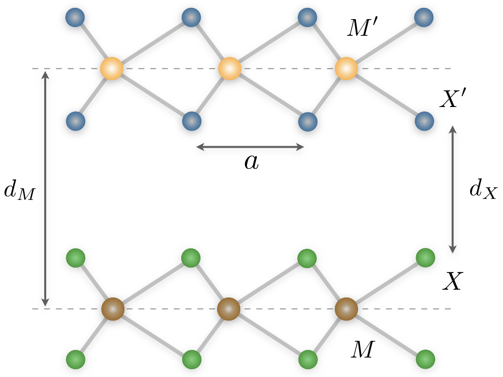
(a)

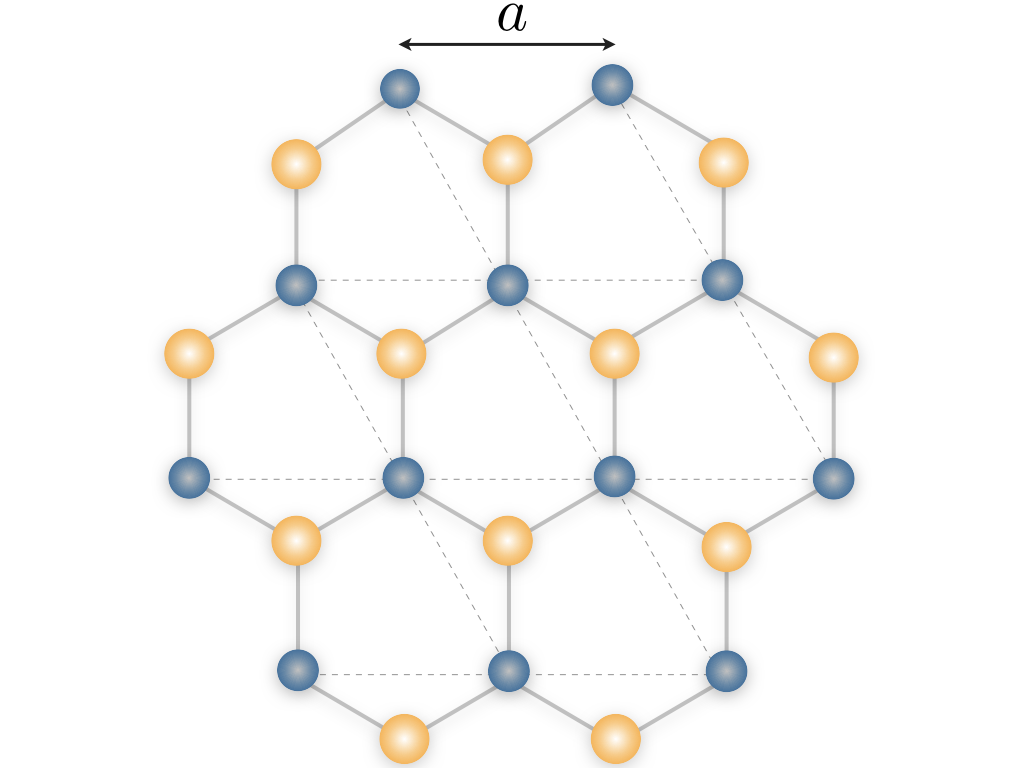
(b)

Figure 1: Schematic of AA stacked TMD bilayer: (a) the side-view shows the $MX_{2}$ layer, with trigonal prismatic (H) coordination, stacked on top of the $M^{\prime}X^{\prime}_{2}$ layer. The large (yellow or brown) balls represent the metal ions, $M$ or $M^{\prime}$, and the small (blue or green) balls represent the chalcogens, $X$ or $X^{\prime}$. The distance between the metal ions and the chalcogens are, respectively, denoted by $d_{M}$ and $d_{X}$. (b) The top-view is a honeycomb lattice of lattice of lattice constant $a$.

Typically, a pure WC formed in a 2DEG slides when subjected to a nonzero electric field due to the lack of a momentum relaxation mechanism. A key signature of such a WC is its negative compressibility Eisenstein et al. (1992); Li et al. (2011); Skinner and Shklovskii (2010); Bello et al. (1981); Chitra et al. (2001). Disorder, however, pins the WC and renders it incompressible as a result of the activation or pinning gap. A WC realized in moiré materials Padhi et al. (2018); Padhi and Phillips (2019) is however, ineluctably influenced by the underlying moiré lattice, which provides a uniform periodic background potential as illustrated in Fig. 2. This provides a pinning mechanism distinct from that induced by disorder which will strongly influence its properties. Such a crystal is often referred to as a ‘generalized Wigner crystal’ (GWC) Hubbard (1978), see Fig. 2. Although disorder-pinned-WCs have been studied widely Grimes and Adams (1979); Monarkhaa and V. E. Syvokon (2012); Chen et al. (2003); Jang et al. (2017); Hatke et al. (2015); Monceau (2012); Delacrétaz et al. (2019), an in-depth study of GWCs is still lacking.

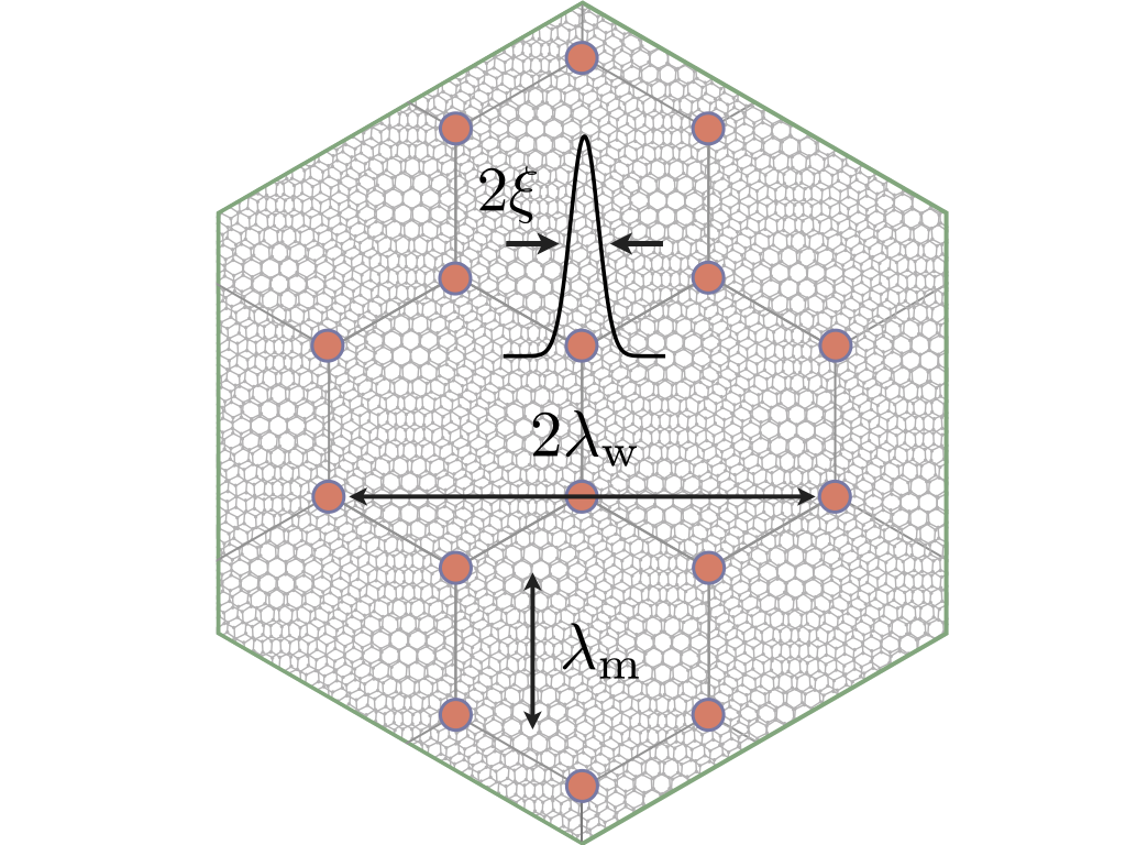
Figure 2: A cartoon rendition of a WC and the relevant length scales: A Wigner lattice is realized on a moiré superlattice (gray background) at filling fraction $2/3$. The distance between two nearest dark (or bright) spots is the moiré periodicity, $\lambda_{\mathrm{m}}$. The distance between the two nearest localized particles (red dots) is the Wigner lattice periodicity, $\lambda_{\mathrm{w}}$. The bell-shaped curve, representing the wavefunction of a localized particle, has a width of $2\xi$. Our discussion in this paper is confined to a crystal where the moiré electrons are highly localized, $\xi\ll\lambda_{\rm w}$.

In light of the recent experiments in TMD platforms exploring the physics of strong correlations Regan et al. (2020); Xu et al. (2020); Jin et al. (2020); Shimazaki et al. (2020a, b), a study of the properties of the GWC is timely as it helps distinguish the GWC from other density ordered gapped states that a lattice system may host alongside a GWC Noda and Imada (2002); Jin et al. (2020); Slagle and Fu (2020); Shimazaki et al. (2020b); Pan et al. (2020). Insulating states observed in $\rm WSe_{2}/WS_{2}$ are at fractional fillings, $\nu=1/3,2/3$, Regan et al. (2020) and those in the twisted bilayer of graphene (TBLG) are at integer fillings Cao et al. (2018a, b); Yankowitz et al. (2019); Lu et al. (2019); Kerelsky et al. (2018); Choi et al. (2019); Wong et al. (2020); Zondiner et al. (2020); Stepanov et al. (2019). Simple observables like compressibility (or capacitance) are often misguiding and insufficient Tomarken et al. (2019); Camjayi et al. (2008); Eisenstein et al. (1994); Zhang et al. (2014) to discern between a pinned WC and a Mott state as these exhibit similar capacitive signatures Eisenstein et al. (1994); Zhang et al. (2014). However, in the presence of the moiré lattice, Mott states must preserve the underlying (moiré) lattice symmetry, and can only be observed at fillings for which a placement of the electrons preserves the underlying symmetry of the moiré lattice. While this is difficult for integer fillings exceeding unity Padhi et al. (2018); Padhi and Phillips (2019), it is impossible at fractional filling observed in $\rm WSe_{2}/WS_{2}$. Consequently, the nature of the insulating states at integer fillings remains ambiguous. In TBLG, our earlier works Padhi et al. (2018); Padhi and Phillips (2019), based on the Mott criterion, precluded the interpretation of the observed insulating states at integer fillings as Mott states. Wigner crystallization Padhi et al. (2018); Padhi and Phillips (2019) was envisaged to be more favorable than Mott insulation at low charge densities in TBLG.

In this paper, we explore from a materials perspective the viability of both homo- and hetero-bilayer TMDs for realizing WCs . Additionally, we study the impact of the moiré lattice on collective excitations Grimes and Adams (1979); Monarkhaa and V. E. Syvokon (2012); Chen et al. (2003) of GWCs and present estimates for the gap in the deep crystalline limit which can be directly accessed in transport experiments. Our results are directly of relevance to a slew of recent experiments in these systems exploring the physics of the GWC Regan et al. (2020); Shimazaki et al. (2020a). We organize this article as follows. In Sec. II, we analyze the material parameters of various HoM and HeM systems and assess their candidacy for crystal formation using several criteria. We identify a wide range of TMD materials that can support GWC phases and establish, broadly speaking, HeM to be better candidates than HoM for this purpose. In Sec. III, in the elastic limit Giamarchi and Le Doussal (1995, 1997); Chitra et al. (2001), we obtain an effective Hamiltonian that describes harmonic fluctuations in a GWC pinned to a moiré lattice. We then move to obtaining the self-consistent equations for the pinning gaps corresponding to a GWC in Sec. IV. Finally, we conclude by connecting our results to the recent experiments in Sec. V. Technical details are relegated to various appendices.

II TMD Candidacy For Wigner Crystallization

In this section, we discuss the key criteria for assessing the candidacy of various TMD bilayers, both HoM and HeM for Wigner crystallization. Generally, a material with low carrier density and a high degree of correlation can be susceptible to forming a WC. A natural way to measure correlation is to compare the strength of electronic interaction ($U$) with the kinetic energy ($W$) of the relevant charge carriers. Assuming the mean separation between the moiré particles to be of the order of the moiré periodicity, $\lambda_{\mathrm{m}}$, we set the scale of the Coulomb repulsion to $U={e^{2}}/{\epsilon\lambda_{m}}$, where, $e$ is electronic charge and $\epsilon$ is the dielectric constant. In principle, one can also use a more realistic interaction potential for TMDs that can account for the encapsulating environment (such as the $\rm hBN/SiO_{2}$ surroundings) Cudazzo et al. (2011); Danovich et al. (2018); Scharf et al. (2019). However, at long distances, such a potential distills to a Coulomb-type potential Yang et al. (1991). Therefore, our assumption remains useful for discussing the low energy physics of TMDs. Another simplifying assumption we make is to ignore the full details of the TMD bandstructure Wu et al. (2019, 2018). We simply set $W={\hbar^{2}k^{2}}/{2m^{e}_{\ast}}$ with $k\simeq\pi/\lambda_{\mathrm{m}}$. $m^{e}_{\ast}$ ($m^{h}_{\ast}$) is the effective mass of the electrons (holes) in the conduction (valence) band. We will later see that typically, $W\sim\mathcal{O}(1\,\text{meV})$ and $U\sim\mathcal{O}(10\,\mathrm{meV})$.

Here, we reiterate that the important (in-plane) length scales in the problem, as shown in Figs. 1 and 2, are – the monolayer lattice constant ($a$), the moiré periodicity ($\lambda_{\rm m}$), the Wigner lattice periodicity ($\lambda_{\rm w}$), and the localization length of the moiré particles ($\xi$). $a$ is the smallest scale and can be neglected in a low energy theory. $\lambda_{\rm m}$ is a geometric scale which is fixed for a given TMD device. Unlike these two lengths, $\xi$ and $\lambda_{\rm w}$ are dynamically generated. By working in the deep crystalline limit where $\xi\ll\lambda_{\rm m},\lambda_{\rm w}$ we can drop $\xi$. Thus, the most important scale in our problem is $\lambda_{\rm w}$, and its interplay with $\lambda_{\rm m}$. Since $\lambda_{\rm w}=1/\sqrt{\pi n_{e}}$ is a function of electronic density $n_{e}$ (or hole density $n_{h}$), it allows us to study crystallization as a function of doping levels. Using this, the kinetic $(W)$ and potential $(U)$ energies can be recast as $W^{-1}=2m\pi n_{e}$ and $U^{-1}=\epsilon\sqrt{\pi n_{e}}$. The dimensionless ratio of these two parameters, also known as $r_{s}$, provides crucial insight into nature of a correlated state Tanatar and Ceperley (1989). Ignoring the effect of the moiré potential on the energies, we obtain

$$r_{s}=\frac{\rm g}{a_{0}m_{0}}\frac{m^{e}_{\ast}}{\epsilon}\lambda_{\rm w}\quad,\quad\lambda_{\rm w}=\frac{1}{\sqrt{\pi n_{e}}},$$ (1)

where $a_{0}=\hbar^{2}/m_{0}e^{2}=0.529\,\rm{\AA}$ is the Bohr radius with $m_{0}$ as the bare electron mass. And, $\mathrm{g}=2$ is a valley degeneracy factor for TMDs. This valley degree of freedom can significantly alter the correlation properties and the threshold for Wigner crystallization. In a 2-valley 2DEG the crystallization threshold drops to $r_{s}=29.5$ Zarenia et al. (2017) from $r_{s}=37$ in a 1-valley system Tanatar and Ceperley (1989); Drummond and Needs (2009). The further $r_{s}$ exceeds this threshold value, the easier it is to form a WC. For further discussion on a more fine-tuned definition of $r_{s}$, see Padhi and Phillips (2019). Note however, due to the availability of a set of potential minima facilitated by the underlying moiré lattice, the threshold value for GWCs could be lower than $r_{s}=29.5$.

Clearly, Eq. (1) shows that the material parameters that favor Wigner crystallization (or enhance $r_{s}$) are a high effective mass, reduced screening or a small dielectric constant and low carrier density. Firstly, low energy carriers in TMDs or twisted bilayers of TMDs are particularly heavy. Secondly, though the dielectric constant of a material is fixed, it can be altered by introducing a spacer layer Shimazaki et al. (2020a), such as a hexagonal boron nitride (hBN) monolayer. Screening can then be reduced by a judicious choice of spacer material , thereby favoring Wigner crystallization.

Evidently however, the moiré scale dependence of $r_{s}$ is not manifest in Eq. (1). This can be naturally restored by measuring the carrier density through the filling fraction of a moiré unit supercell. This can be understood as follows. The area of a (hexagonal) moiré unit supercell is given by $A_{s}=\sqrt{3}\lambda_{\mathrm{m}}^{2}/2$. If the full occupancy of the relevant low energy band is $N_{0}$, usually determined by the discrete symmetries of the system, then the supercell density is given by $n_{s}=N_{0}/A_{s}\sim 10^{11\text{-}12}$ cm${}^{\text{-}2}$. A state consisting of $N$ electrons in this band is observed at a filling fraction of $N/N_{0}\equiv\nu$, or at a density $n_{e}=\nu n_{s}$. Inserting this in Eq. (1), we observe that, for a given material, there exists a critical density, $n_{e}^{\rm max}$, or a maximal filling fraction, $\nu_{\rm max}$, above which a GWC cannot exist. Correspondingly, since $r_{s}\propto\lambda_{m}$ [replacing $\lambda_{\rm w}$ with $\lambda_{\rm m}$ in Eq. (1)], there also exists a critical moiré length below which a material cannot host a GWC. It is worth noting here that the true advantage of moiré materials in realizing WC is this availability of large length scales that govern most of the physics.

Before proceeding further, we note the above discussions are pertinent for zero temperature WC (or quantum WC) only. As the temperature increases, one needs to confront the problem of crystal melting. Although an accurate estimation of this melting temperature can be a subtle issue Illing et al. (2017); Khrapak (2020); Ma et al. (2020), for simplicity, we estimate it using the classical Lindemann criterion, $k_{B}T_{\mathrm{L}}\simeq 0.01U$. Our discussions in this paper will be confined to the physics of a GWC at $T\ll T_{\mathrm{L}}$. In the subsections below, we will explicitly evaluate all the above mentioned parameters for several TMDs.

II.1 Homobilayers

Table 1: Wigner crystallization criteria for HoMs: The effective mass of the conduction band ($m_{e}^{\ast}$) is obtained using DFT-LDA in Ref. Kormányos et al. (2015). Monolayer and bilayer dielectric constants ($\epsilon_{\perp},\epsilon_{\parallel}$ and $\epsilon_{\perp}^{(2)},\epsilon_{\parallel}^{(2)}$) are adapted from Ref. Kumar and Ahluwalia (2012). Experimental lattice constant ($a$) data and the distance between the TMD layers ($d_{X}$) are compiled in Ref. Kormányos et al. (2015). For this table, we set the twist angle to $\theta=1^{\circ}$. Eq. (1) reduces to $r_{s}=674{m_{e}^{*}}/{m_{0}\epsilon}$ for $n_{e}=10^{11}$cm${}^{\text{-}2}$, which we also use as the unit for densities mentioned thereafter. The critical density, or the closest rational filling fraction, $\nu_{\rm max}=n_{e}^{\rm max}/n_{s}$, below which a HoM system can host GWC is obtained by setting $r_{s}=29.5$ in Eq. (1). The Lindemann melting temperature ($T_{\rm L}$) of a GWC and the density ($n_{\rm Mott}$) for which the Mott criterion is satisfied are obtained in the end. We observe that due to the larger effective masses, the $\rm Mo$-based compounds are generally better suited to forming GWCs as compared to the $\rm W$-based compounds. In regard to $r_{s}$, or $U/W$, we conclude a twisted bilayer of $\rm MoSe_{2}$ to be the best candidate for Wigner crystallization.

HoMs	${\rm MoS_{2}}$	$\rm MoSe_{2}$	$\rm MoTe_{2}$	$\rm WS_{2}$	$\rm WSe_{2}$	$\rm WTe_{2}$
$m_{\ast}^{e}/m_{0}$	$0.46$	$0.56$	$0.62$	$0.26$	$0.28$	$0.26$
$\epsilon_{\perp}(\epsilon_{\parallel})$	$4.8(3.0)$	$6.9(3.8)$	$8(4.4)$	$4.4(2.9)$	$4.5(2.9)$	$5.7(3.3)$
$\epsilon^{(2)}_{\perp}(\epsilon^{(2)}_{\parallel})$	$6.9(4.4)$	$7.9(4.6)$	$8.6(5.5)$	$6.1(4.2)$	$6.3(4.3)$	$8.4(5.2)$
$d_{X}$ [Å]	$3.17$	$3.33$	$3.60$	$3.14$	$3.34$	$3.60$
$a$ [Å]	$3.16$	$3.29$	$3.52$	$3.15$	$3.28$	$3.50$
$\lambda_{\mathrm{m}}$ [nm]	$18.1$	$18.8$	$20.2$	$18.0$	$18.8$	$20.0$
$U/W$	$5.0$	$5.8$	$6.0$	$3.1$	$3.3$	$2.6$
$r_{s}\rvert_{10^{11}\text{cm}^{\text{-2}}}$	$56.3$	$62.6$	$60.8$	$34.7$	$36.3$	$26.5$
$n_{e}^{\rm max}$	$3.6$	$4.5$	$4.2$	$1.4$	$1.5$	$0.8$
$\nu_{\rm max}$	$1.02$	$1.38$	$1.48$	$0.40$	$0.46$	$0.28$
$T_{\mathrm{L}}$ [K]	$1.7$	$1.5$	$1.2$	$1.8$	$1.7$	$1.3$
$n_{\rm Mott}10^{-3}$	$2.5$	$3.1$	$2.9$	$0.9$	$1.0$	$0.6$

In a HoM system, the top and the bottom layers consist of the same TMD where each layer projects to a 2D honeycomb lattice (see Fig. 1b). This, therefore, is geometrically equivalent to a twisted bilayer graphene system. The moiré periodicity in a HoM is thus given by Lopes dos Santos et al. (2007) $\lambda_{\mathrm{m}}(\theta)=\frac{a}{2\sin(\theta/2)}\simeq a/\theta$. Here, $\theta$ is the twist angle between the two TMD layers. ($\epsilon_{\mkern 3.0mu\vphantom{\perp}\vrule depth=0.0pt\mkern 2.0mu\vrule depth=0.0pt\mkern 3.0mu}^{\phantom{2}},\epsilon_{\perp}^{\phantom{2}}$) and ($\epsilon_{\mkern 3.0mu\vphantom{\perp}\vrule depth=0.0pt\mkern 2.0mu\vrule depth=0.0pt\mkern 3.0mu}^{2},\epsilon_{\perp}^{2}$) denote the in-plane and out of plane dielectric constants of a monolayer and a homobilayer TMD respectively. We identify the geometric mean of these two constants, $\epsilon^{(2)}=\sqrt{\epsilon^{(2)}_{\perp}\epsilon^{(2)}_{\mkern 3.0mu\vphantom{\perp}\vrule depth=0.0pt\mkern 2.0mu\vrule depth=0.0pt\mkern 3.0mu}}$, as the dielectric constant of the bilayer system Mak et al. (2013).

Using these parameters, we summarize our results for crystallization criteria in different candidate HoMs in Table 1. For a typical twist angle $\theta=1^{\circ}$, we find that, $U/W>1$ for all the homobilayers in Table 1, rendering them strongly interacting systems. The corresponding $r_{s}$ computed using Eq. (1) shows that all the HoMs in Table 1 are susceptible to forming GWCs since they all have $r_{s}$ fairly above the crystallization threshold. The critical density for crystallization is found to be nearly the order of $n_{s}$. The filling fraction ($\nu_{\rm max}$) below which the GWCs can be observed are also evaluated along with it. Based on the Lindemann criteria, our results predict that the GWCs should be stable in the range of $1$K-$3$K. Our simple analysis shows that $\rm Mo$-based HoMs are more viable than $\rm W$-based compounds for the realization of GWCs.

Finally, we evaluate the Mott criterion, , $n_{e}^{1/2}a_{0}^{\ast}\approx O(1)$, which a system needs to satisfy in order to host Mott insulating states Mott and Davis (2012). The effective Bohr radius, $a_{0}^{\ast}=\hbar^{2}/m^{e}_{\ast}e_{\ast}^{2}$ and $e_{\ast}=e^{2}/\epsilon$. Evalutating this for HoMs, we find that for experimentally relevant densities (that is near the fractional fillings of a moiré unit supercell) the Mott criterion is far from being met, $n_{e}^{1/2}a_{0}^{\ast}\sim\mathcal{O}(10^{-2})\ll 1$. Satisfying the Mott criterion, $n_{\rm Mott}^{1/2}a_{\ast}=1$ requires densities nearly three orders of magnitude larger than the maximal density for GWC formation. This indicates that for the typical density of operation, HoM systems are far from the Mott insulating regime.

Table 2: Wigner crystallization criteria for a nearly-aligned HeMs: Any experimental study of the pertaining heterostructure is referenced here. The electron (hole) effective mass $m_{e}(m_{h})$ are adapted from Ref. Xu et al. (2018). The moiré length is evaluated following Eq. (2). Like before, we set the twist angle to $\theta=0.5^{\circ}$ and the particle density to $n_{e}=10^{12}\rm cm^{-2}$. Asterisked values in the $r_{s}$ row indicate values crossing the crystallization threshold. Note that the Lindemann temperature is the same for both electron and hole crystals since $U$, under our assumptions, simply depends on the geometry and not on the effective mass. Since the hole bands have higher effective mass they display larger correlation than the electron bands. In particular, among the heterobilayers listed here, $\rm MoSe_{2}/WSe_{2}$ and $\rm MoS_{2}/WS_{2}$ seem to be the most susceptible to forming an electronic and hole GWC, respectively.

HeMs	$\rm WSe_{2}/WS_{2}$	$\rm MoSe_{2}/MoS_{2}$	$\rm MoTe_{2}/MoSe_{2}$	$\rm MoSe_{2}/WS_{2}$	$\rm MoSe_{2}/WSe_{2}$	$\rm MoS_{2}/WS_{2}$	$\rm MoTe_{2}/WSe_{2}$
Refs.	Regan et al. (2020); Jin et al. (2019)	Zhang et al. (2018)	Kozawa et al. (2016); Alexeev et al. (2019)	Seyler et al. (2019)	Hong et al. (2014); Yang et al. (2018)	Gong et al. (2014)	Yamaoka et al. (2018)
$m_{e(h)}^{*}/m_{0}$	$0.28\,(0.46)$	$0.42\,(0.71)$	$0.46\,(1.37)$	$0.28\,(0.71)$	$0.54\,(0.44)$	$0.46\,(1.70)$	$0.30\,(1.33)$
$2/(\epsilon_{1}^{-1}+\epsilon_{2}^{-1})$	$2.9$	$3.35$	$4.08$	$3.29$	$3.29$	$2.95$	$3.5$
$\lambda_{\mathrm{m}}$ [nm]	$8.1$	$8.1$	$5.3$	$7.6$	$35.6$	$34.0$	$5.1$
$U/W\rvert_{e(h)}$	$3.0\,(4.9)$	$3.9\,(6.6)$	$2.3\,(6.9)$	$2.5\,(6.3)$	$22.4\,(18.2)$	$20.3\,(75.1)$	$1.7\,(7.5)$
$r_{s}^{e(h)}\rvert_{10^{12}\text{cm}^{\text{-2}}}$	$20.6\,(33.8^{*})$	$26.7\,(45.2^{*})$	$24.0\,(71.6^{*})$	$18.2\,(46.0^{*})$	$35.0^{*}\,(28.5)$	$33.3^{*}\,(122.9^{*})$	$18.3\,(81.1^{*})$
$T_{\mathrm{L}}$ [K]	$7.1$	$6.1$	$7.6$	$6.7$	$1.4$	$1.7$	$9.3$
$n_{e(h)}^{\rm max}\,[10^{12}$ cm${}^{\text{-}2}$]	$0.5\,(1.3)$	$0.8\,(2.3)$	$0.7\,(5.9)$	$0.4\,(2.4)$	$1.4\,(0.9)$	$1.3\,(17.4)$	$0.4\,(7.5)$
$\nu_{\rm max}^{e(h)}$	$0.28\,(0.73)$	$0.46\,(1.31)$	$0.17\,(1.46)$	$0.2\,(1.19)$	$15.56\,(10.0)$	$13.0\,(174.0)$	$0.09\,(1.7)$

II.2 Heterobilayers

In HeM materials, the top and bottom layers contain different TMDs. We now explore the potential for GWCs in HeMs in the manner done in the preceding section for homobilayers. Although the planar projection of each layer is a honeycomb lattice with different periodicities, a moiré pattern emerges even without introducing any twist angle (‘near-aligned sample’). Twisting alters the moiré periodicity; in particular, it reduces with increasing twist angle and often approaches the original lattice constant at ‘large-twist-angles’. For example, in a HeM with a small difference in lattice constants  Lu et al. (2014), the moiré periodicity is  Jin et al. (2019); Ruiz-Tijerina et al. (2020)

$$\lambda_{m}\simeq\frac{a_{>}}{\sqrt{\delta_{a}^{2}+4\sin^{2}(\theta/2)}}\quad,\quad\delta_{a}=1-\frac{a_{<}}{a_{>}}.$$ (2)

Here $a_{>(<)}$ is the largest (smallest) lattice constant among the two layers. We see that $\lambda_{m}$ is strongly influenced by the twist angle for samples with small $\delta_{a}$. As shown inTable 1, this is the case of HeMs with differing metal ions [$\mathit{MX_{2}/M^{\prime}X_{2}}$] which have $\delta_{a}\lesssim 0.1\%$. HeMs with differing chalcogens [${\mathit{MX_{2}/MX^{\prime}_{2}}}$] tend to have large $\delta_{a}$, i.e. around $4\%$ and are less sensitive to small angle twists. Motivated by the experiment of Ref. Regan et al. (2020) which concern $\theta\lesssim 1^{\circ}$ Jin et al. (2019), we confine our discussion to nearly-aligned heterobilayers.

The effective dielectric constant of the HeM system is obtained by treating the two layers as two dielectrics (or capacitors) in series,

$$\frac{d_{1}+d_{2}}{\epsilon}=\frac{d_{1}}{\epsilon_{1}}+\frac{d_{2}}{\epsilon_{2}},$$ (3)

where $\epsilon_{i}$ and $d_{i}$ are the dielectric constants and the thickness of the top and bottom layers, respectively. We assume $d_{1}=d_{2}$ and as the two layers are different and stacked along the direction that is normal to the dielectric plane, we set $\epsilon_{i}$ to be the in-plane monolayer dielectric constants, $\epsilon_{{\mkern 3.0mu\vphantom{\perp}\vrule depth=0.0pt\mkern 2.0mu\vrule depth=0.0pt\mkern 3.0mu},i}$. For near-aligned samples with $\theta=0.5^{\circ}$, using Eq. (2) and Eq. (1) we evaluate $U/W$ and $r_{s}$ for different HeMs. Our results are summarized in Table 2. We find generically that hole carriers have larger $r_{s}$ due to their larger effective masses. Almost all the HeMs considered in Table 2 can Wigner crystallize for a hole density of $10^{12}$ cm${}^{\text{-}2}$or less. However, except for a few, most of the electronic carriers do not crystallize.

Since $\rm MoSe_{2}/WSe_{2}$ and $\rm MoS_{2}/WS_{2}$ share the same chalcogens, they are quite sensitive to twist angle. For $\theta\sim 0^{\circ}$, the moiré length can be as large as a micrometer and it gradually reduces to about a deca-nanometer by $5^{\circ}$ of twisting. The correlation factor $U/W$, therefore, also reduces by nearly two orders of magnitude. For the remainder of the HoMs, though the above mentioned trend is still valid, however, quantitatively, no significant change is observed in the correlation factor since the moiré length scale remains largely insensitive to small changes in the twist angle. In particular, for $\rm WSe_{2}/WS_{2}$, we find that at filling fraction $\nu=1/3$, $r_{s}=44.0$ ($26.8$) for holes (electrons), and at $\nu=2/3$, it is $31.1$ ($19.0$) for holes (electrons). This thus explains why Regan et al. Regan et al. (2020) observe GWC states on the hole side but not on the electronic side. This is one of our key results as it bares directly on the experiments.

Lastly, we evaluate the critical density, or filling fraction, above which the heterostructure will be unable to host GWCs. In particular, for $\rm WSe_{2}/WS_{2}$ we observe that no hole-crystal can exist above a filling fraction of $0.73\,(\approx 3/4)$. States at any filling fraction below this, even other than those at $1/3$ and $2/3$ Slagle and Fu (2020), are perfectly allowed. Similarly, on the electron side, GWC can exist up to $\nu=0.28\,(\approx 1/4)$.

To summarize, based on the best estimates of the system parameters, we find a variety of homobilayer and heterobilayer TMDs to be excellent candidates for realizing WCs. In particular, our analysis based on $r_{s}$ indicates that $\rm MoSe_{2}$ (among the homobilayers) and $\rm MoSe_{2}/WSe_{2}$ or $\rm MoS_{2}/WS_{2}$ (among the heterobilayers) are the best candidates for realizing WCs. We also establish that due to larger effective masses of the valence bands, hole-crystals in general, are easier to realize than electron-crystals, an observation consistent with experiments. In the remainder of the paper, we focus on the properties of a GWC.

III Effective Theory of GWC

Understanding the collective excitations of a GWC is critical in distinguishing them from the other density ordered states observed in the lattice system. Here, we will focus on the vibrational modes of the GWC in absence of an external magnetic field. For analytical tractability we will confine our discussion to the limit when the GWC is deep in the crystalline regime. We represent the particle density of the system using a lattice of Gaussian wave-packets of size $2\xi$ (see Fig. (2)),

$$\begin{split}\rho(\boldsymbol{x})&=\sum_{i}|\psi\left(\boldsymbol{x}-\boldsymbol{R}_{i}\right)|^{2},\\ |\psi(\boldsymbol{x})|^{2}&=\frac{1}{2\pi\xi}\exp\left(-|\boldsymbol{x}^{2}|/{4\xi^{2}}\right).\end{split}$$ (4)

where $\boldsymbol{R}_{i}=\boldsymbol{R}_{i}^{0}+u_{i}(t)$, describes fluctuations around the mean lattice sites $\boldsymbol{R}_{i}^{0}$. The GWC we consider is far away from the phase boundary with the liquid phase so that we can treat the mean fluctuation in the position of the localized electrons, $\langle\boldsymbol{r}^{2}\rangle\sim\xi^{2}$, to be much smaller than the Wigner lattice periodicity, $\xi\ll\lambda_{\mathrm{w}}$, as in Fig. 2. Since the field $\boldsymbol{u}_{i}(t)$ measures the fluctuation around the mean position of a particle, it is naturally $\mathcal{O}(\xi)$. For a GWC at $T=0$, $\xi$ (hence, $\boldsymbol{u}_{i}$) can be tuned by changing the density alone. A self-consistent solution of $\xi$ as a function of density is discussed in Ref. Chitra and Giamarchi (2005). Finally, since $\xi$ increases with increasing temperature, we will restrict our discussion to low temperature, $T\ll T_{\mathrm{L}}$.

In this regime, the above density functional can be written in terms of harmonics (see App. A for a derivation)

$$\rho(\boldsymbol{x})\simeq\rho_{0}\Big{[}1-\boldsymbol{\nabla}\cdot\boldsymbol{u}(\boldsymbol{x})+\sum_{l\neq 0}e^{i\boldsymbol{K}_{l}\cdot\boldsymbol{x}}\rho_{l}(\boldsymbol{x})\Big{]}.$$ (5)

Here, $\rho_{l}(\boldsymbol{x})=e^{-i\boldsymbol{K}_{l}\cdot\boldsymbol{u}(\boldsymbol{x})}$ and $\rho_{0}$ is the average density (over the entire sample). The second term accounts for long range density fluctuations over several $\lambda_{\mathrm{w}}$ and couples to couples to the long-range (or $q\sim 0$) component of the Coulomb interaction. The remaining terms take care of the density fluctuations at a length scale comparable to or smaller than $\lambda_{\mathrm{w}}$ and hence can be referred to as un-smeared density. The wave vectors $\boldsymbol{K}_{l}=\{\pm l\boldsymbol{\kappa}_{n}\}$ denote the Brillouin zone (BZ) vectors of the undeformed GWC. Here, $l=1,2,\cdots$ are simply ‘size multipliers’ of the BZ. Formally, the $l=0$ term is nothing other than $\rho_{0}$ in Eq. (5). The last term above also contains a summation over the index $n$ appearing through $K_{l}$. We perform this summation implicitly since it does not play any significant role in our analysis.

The long wavelength theory describing the fluctuations of the crystal is given by an elastic Hamiltonian

$$H_{\mathrm{eff}}=\frac{1}{2}\sum_{\omega_{n}}\int\frac{d^{2}\boldsymbol{q}}{(2\pi)^{2}}u_{\alpha}(\boldsymbol{q},\omega_{n})\,\Phi_{\alpha\beta}(\boldsymbol{q},\omega_{n})\,u_{\beta}(-\boldsymbol{q},-\omega_{n}),$$ (6)

where $\alpha,\beta=x,y$ are summed over, momenta $\{\boldsymbol{q}\}$ form the Fourier basis, and the kernel $\Phi_{\alpha\beta}(\boldsymbol{q},\omega_{n})$ is the elastic matrix. Henceforth, we will express all the quantities after performing the frequency ($\omega_{n}$) summation. In case of a classical ($\omega_{n}=0$) free theory, this matrix is $\Phi_{\alpha\beta}=cq^{2}\delta_{\alpha\beta}$, with the real space Hamiltonian $H_{\mathrm{eff}}=\frac{c}{2}\int d^{2}\boldsymbol{x}\left[\boldsymbol{\nabla}\cdot\boldsymbol{u}(\boldsymbol{x})\right]^{2}$. Here $c$ is an elastic modulus. The presence of the moiré potential and the Coulomb interaction between the particles generates the following terms in the hamiltonian

$$H_{1}=H_{\mathrm{e}\text{--}\mathrm{l}}+H_{\mathrm{e}\text{--}\mathrm{e}},$$ (7)

where electron-moiré lattice interaction and the electron-electron interaction terms, respectively, are

$$H_{\mathrm{e}\text{--}\mathrm{l}}=-\int_{\boldsymbol{x}}\,V(\boldsymbol{x})\rho(\boldsymbol{x}),$$ (8a)

$$H_{\mathrm{e}\text{--}\mathrm{e}}=\frac{1}{2}\int_{\boldsymbol{x},\boldsymbol{x}^{\prime}}\,U(\boldsymbol{x}-\boldsymbol{x}^{\prime})[\rho(\boldsymbol{x})-\rho_{0}][\rho(\boldsymbol{x}^{\prime})-\rho_{0}]\,.$$ (8b)

We will approximate the (triangular) moiré potential, $V(\boldsymbol{x})$, by Wu et al. (2019); Zhang et al. (2019)

$$V(\boldsymbol{x})=2\tilde{V}\sum_{m=1}^{3}\cos\left(\boldsymbol{x}\cdot\boldsymbol{g}_{m}+\phi\right),$$ (9)

where $\tilde{V}\sim\mathcal{O}(10\,\text{meV})$ sets the depth of the moiré potential and $\phi$ determines the shape of the potential. These two (intrinsic) parameters can be fixed for a given TMD using methods developed in Ref. Zhang et al. (2019). Lastly, the unit vectors of the moiré Brillouin zone (MBZ) are given by $\boldsymbol{g}_{m}=\frac{4\pi}{\sqrt{3}\lambda_{\mathrm{m}}}\left(\cos\frac{2\pi m}{3},\sin\frac{2\pi m}{3}\right)$.

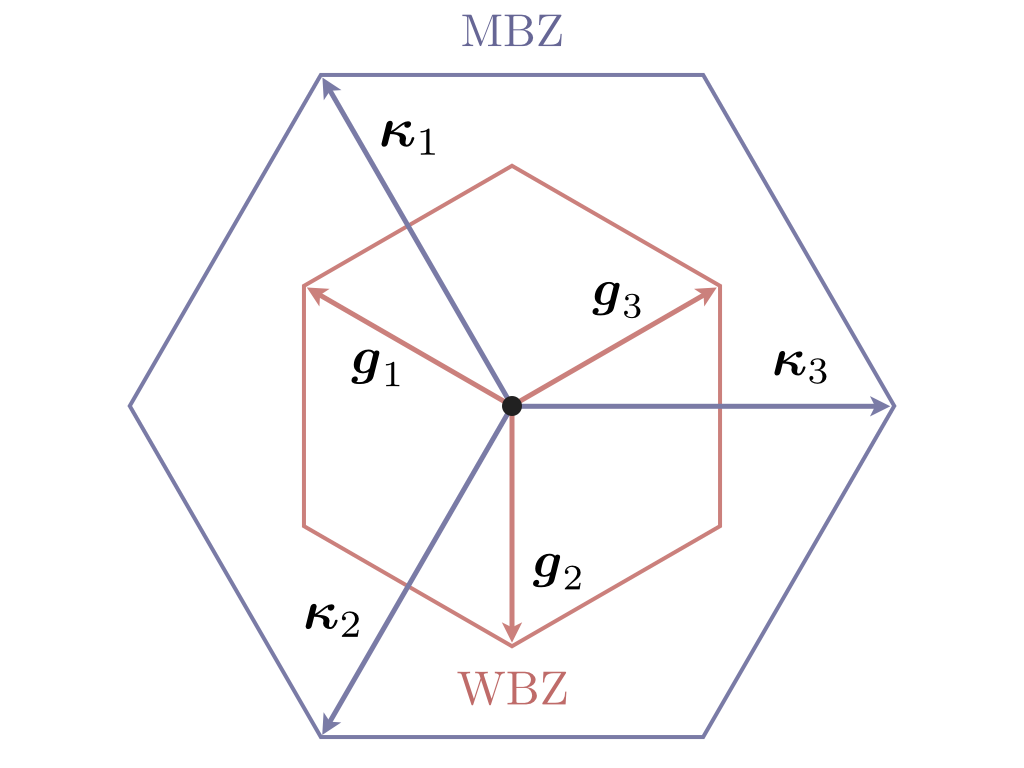
Figure 3: Schematic of a moiré BZ (MBZ, blue) and a Wigner BZ (WBZ, red). The BZ vectors are, $g_{n}=\frac{4\pi}{\sqrt{3}\lambda_{\rm m}}\left(\cos\frac{2\pi n}{3},\sin\frac{2\pi n}{3}\right)e^{i\pi/6}$ and $\kappa_{n}=\frac{4\pi}{\sqrt{3}\lambda_{\rm w}}\left(\cos\frac{2\pi n}{3},\sin\frac{2\pi n}{3}\right)$. In general, since $\lambda_{\rm w}>\lambda_{\rm m}$, the WBZ is smaller than the MBZ. For the particular case drawn above, $\lambda_{\rm w}=3\lambda_{\rm m}$. In other words, the third WBZ is the same as the first MBZ ($|\boldsymbol{\kappa}_{n}|=3|\boldsymbol{g}_{n}|$).

III.1 Interaction with the moiré potential

We now focus on the moiré potential given by the first term term in Eq. (7). In terms of a reciprocal vector of the MBZ, $\boldsymbol{G}_{m}=\{\pm m\boldsymbol{g}_{n}\}$, where $\boldsymbol{g}_{n}$ are the primitive MBZ vectors, see Fig. 3, the periodic moiré potential is Wu et al. (2019); Jin et al. (2019)

$$V(\boldsymbol{x})=\sum_{m}V_{m}\,e^{i\boldsymbol{G}_{m}\cdot\boldsymbol{x}}.$$ (10)

As before, $m$ is a size multiplier for the principal MBZ and a summation over the index $n$ is made implicit. We assume the potential to be an even function in position space and set the $m=0$ mode to zero. For the potential in Eq. (9), we obtain $V(\boldsymbol{G}_{m})=\tilde{V}e^{i\mathrm{sgn}(m)\phi}$. Substituting Eq. (10) in Eq. (8a), we obtain the following moiré term

$$H_{\mathrm{e}\text{--}\mathrm{l}} =-\rho_{0}\sum_{l,m}\,V_{m}\,\int d\boldsymbol{x}\,e^{i(\boldsymbol{K}_{l}-\boldsymbol{G}_{m})\cdot\boldsymbol{x}}\,\rho_{l}(\boldsymbol{x}).$$ (11)

In writing the above expression, we have set the energy of the moiré lattice, $\sim\int_{\boldsymbol{x}}V(\boldsymbol{x})$, to zero and neglected the gradient term in the density as this term represents an external source term (linear in $\boldsymbol{u}$) and does not contribute to the physics of the pinning gap. Note that the integrand here involves both the WBZ and the MBZ vectors. This term plays a critical role in imposing a certain set of commensuration constraints. In general, a GWC need not conform to the lattice symmetries of a background (e.g., moiré) lattice. With changing density, one often anticipates the GWC to go through a large set of commensurate-incommensurate transitions, also known as the devil’s staircase Bak (1982); Bak and Fukuyama (1980), where the incommensurate structures may also have a completely different lattice symmetry Rademaker et al. (2013) and associated stability issues. These states and the accompanying transitions cannot be described by the elastic (linear harmonic) theory developed here.

In this paper, we focus exclusively on the case where the GWC and the background lattice share the same lattice symmetry, such as in the experiment of Regan et al. Regan et al. (2020). As we will show below, this leads to a geometrical condition $r\boldsymbol{G}_{1}=s\boldsymbol{K}_{1}$, where $(r,s)$ are co-primes and the subscript $1$ refers to the principal BZ vectors. Finally, since usually $\lambda_{\mathrm{w}}\geq\lambda_{\mathrm{m}}$, hence $|\boldsymbol{G}_{1}|\geq|\boldsymbol{K}_{1}|$. As a result, $r\leq s$. For instance, the WC observed in Regan et al. (2020) at $1/3$-filling, or a state at $\nu=1/3^{n}$ in general, simply has its BZ shrunk (without any rotation) by a factor of $2^{n}$. This state of affairs obtains because the GWC at $1/3^{n}$-filling has a unit cell that is $2^{n}$ times larger than that of the moiré lattice. Therefore, for $\nu=1/3^{n}$, $r=1$ and $s=2^{n}$.

III.2 Electronic interaction

Using the underlying translation invariance, we write the interaction term in, Eq. (7) as

$$H_{\mathrm{e}\text{--}\mathrm{e}} =\frac{\rho_{0}^{2}}{2}\int_{\boldsymbol{x},\boldsymbol{x}^{\prime}}U(\boldsymbol{x}-\boldsymbol{x}^{\prime})\left[\boldsymbol{\nabla}\cdot\boldsymbol{u}(\boldsymbol{x})\right]\left[\boldsymbol{\nabla}\cdot\boldsymbol{u}(\boldsymbol{x}^{\prime})\right]+$$

$$\frac{\rho_{0}^{2}}{2}\int_{\boldsymbol{x},\boldsymbol{x}^{\prime}}\sum_{l}U(\boldsymbol{x}-\boldsymbol{x}^{\prime})e^{i\boldsymbol{K}_{l}\cdot(\boldsymbol{x}-\boldsymbol{x}^{\prime})}\rho_{l}(\boldsymbol{x}-\boldsymbol{x}^{\prime}).$$ (12)

Note that terms with $K_{l}\neq K_{m}$ have been discarded as they are highly oscillatory.

We now switch from the cartesian basis $u_{x},u_{y}$ to one described by the longitudinal ($u_{\mkern 3.0mu\vphantom{\perp}\vrule depth=0.0pt\mkern 2.0mu\vrule depth=0.0pt\mkern 3.0mu}$) and transverse ($u_{\perp}$) components with respect to the momentum vectors ($\boldsymbol{q}$)

$$u_{\alpha}(\boldsymbol{q})=u_{\mkern 3.0mu\vphantom{\perp}\vrule depth=0.0pt\mkern 2.0mu\vrule depth=0.0pt\mkern 3.0mu}(\boldsymbol{q})\hat{\boldsymbol{q}}_{\alpha}+u_{\perp}(\boldsymbol{q})\epsilon_{\alpha\beta}\hat{\boldsymbol{q}}_{\beta},$$ (13)

where $\alpha,\beta=\{x,y\}$, and $\epsilon_{\alpha\beta}$ is an antisymmetric tensor, $\epsilon_{xy}=1=-\epsilon_{yx}$. Note that $u_{\mkern 3.0mu\vphantom{\perp}\vrule depth=0.0pt\mkern 2.0mu\vrule depth=0.0pt\mkern 3.0mu}$ and $u_{\perp}$ are the bulk compression and shear modes respectively. In this basis, the first term, $H_{\mathrm{e}\text{--}\mathrm{e}}^{(1)}$, in Eq. (8b) becomes

$$H_{\mathrm{e}\text{--}\mathrm{e}}^{(1)} =\frac{\rho_{0}^{2}}{2}\int_{\boldsymbol{x},\boldsymbol{x}^{\prime}}U(\boldsymbol{x}-\boldsymbol{x}^{\prime})\left[\boldsymbol{\nabla}\cdot\boldsymbol{u}(\boldsymbol{x})\right]\left[\boldsymbol{\nabla}\cdot\boldsymbol{u}(\boldsymbol{x}^{\prime})\right]$$

$$=\frac{d_{\mkern 3.0mu\vphantom{\perp}\vrule depth=0.0pt\mkern 2.0mu\vrule depth=0.0pt\mkern 3.0mu}}{2}\sum_{\boldsymbol{q}}\,q\,u_{\mkern 3.0mu\vphantom{\perp}\vrule depth=0.0pt\mkern 2.0mu\vrule depth=0.0pt\mkern 3.0mu}(\boldsymbol{q})u_{{\mkern 3.0mu\vphantom{\perp}\vrule depth=0.0pt\mkern 2.0mu\vrule depth=0.0pt\mkern 3.0mu}}(-\boldsymbol{q})\quad,\quad\frac{\rho^{2}_{0}e^{2}}{\epsilon}\equiv d_{\mkern 3.0mu\vphantom{\perp}\vrule depth=0.0pt\mkern 2.0mu\vrule depth=0.0pt\mkern 3.0mu}.$$ (14)

We see that the $q=|{\boldsymbol{q}}|$ term results from the long-range (in 2D) nature of the interaction, $U(\boldsymbol{q})\sim 1/q$. Had we considered a shorter-range interaction of the form $U(\boldsymbol{q})\sim 1/q^{\gamma}$, the proportionality above would have been modified to $q^{2-\gamma}$. The transverse modes do not change the local density and remain unaffected by the Coulomb interaction. Typically, long wavelength electrostatic fluctuations, namely the plasma modes, are always longitudinal in the absence of a magnetic field (since $\boldsymbol{q}\times\boldsymbol{E}=0$, where $\boldsymbol{E}$ is an electric field).

In the elastic limit $|\boldsymbol{u}(\boldsymbol{x})-\boldsymbol{u}(\boldsymbol{x}^{\prime})|\ll\lambda_{\mathrm{w}}$, we Taylor expand the second term, $H_{\mathrm{e}\text{--}\mathrm{e}}^{(2)}$, in Eq. (III.2). The first-order term vanishes because the undeformed GWC has an energy minimum at $\boldsymbol{u}=0$ and the second-order term gives the correction

$$H_{\mathrm{e}\text{--}\mathrm{e}}^{(2)}\simeq\frac{\rho_{0}^{2}}{2} \sum_{l}\int_{\boldsymbol{x},\boldsymbol{x}^{\prime}}V(\boldsymbol{x}-\boldsymbol{x}^{\prime})e^{i\boldsymbol{K}_{l}\cdot(\boldsymbol{x}-\boldsymbol{x}^{\prime})}K_{l,\alpha}K_{l,\beta}$$

$$\times\left[u_{\alpha}(\boldsymbol{x})-u_{\alpha}(\boldsymbol{x}^{\prime})\right]\left[u_{\beta}(\boldsymbol{x})-u_{\beta}(\boldsymbol{x}^{\prime})\right]\,.$$ (15)

Here, $\boldsymbol{K}_{l,\alpha}$ denote the $\alpha=x,y$ components of $\boldsymbol{K}_{l}$. Henceforth, unless mentioned, we will set $\rho_{0}=1$.

As shown in App. B, this term can be absorbed into a redefinition of the elastic coefficients  Bonsall and Maradudin (1977); Maki and Zotos (1983); Chitra et al. (2001). We note that we have considered these elastic constants to be $q$-independent, which is a feature of the local elastic theory. One can also extend this analysis to non-local elastic theories where these constants can be considered to be $q$-dependent. Generalizing to an interaction of the form $U(\boldsymbol{x})\sim 1/|\boldsymbol{x}|^{\gamma}$, we find that the full Hamiltonian defining the low energy fluctuations of the GWC can be expressed as

$$H_{\rm eff}=\int_{\boldsymbol{q}}u_{\mkern 3.0mu\vphantom{\perp}\vrule depth=0.0pt\mkern 2.0mu\vrule depth=0.0pt\mkern 3.0mu}(\boldsymbol{q})\,\Omega_{\mkern 3.0mu\vphantom{\perp}\vrule depth=0.0pt\mkern 2.0mu\vrule depth=0.0pt\mkern 3.0mu}u_{\mkern 3.0mu\vphantom{\perp}\vrule depth=0.0pt\mkern 2.0mu\vrule depth=0.0pt\mkern 3.0mu}(-\boldsymbol{q})+u_{\perp}(\boldsymbol{q})\,\Omega_{\perp}u_{\perp}(-\boldsymbol{q})+H_{\mathrm{e}\text{--}\mathrm{l}};$$

$$\Omega_{\mkern 3.0mu\vphantom{\perp}\vrule depth=0.0pt\mkern 2.0mu\vrule depth=0.0pt\mkern 3.0mu}(\boldsymbol{q})=c_{\mkern 3.0mu\vphantom{\perp}\vrule depth=0.0pt\mkern 2.0mu\vrule depth=0.0pt\mkern 3.0mu}q^{2}+d_{\mkern 3.0mu\vphantom{\perp}\vrule depth=0.0pt\mkern 2.0mu\vrule depth=0.0pt\mkern 3.0mu}q^{2-\gamma}\quad,\quad\Omega_{\perp}(\boldsymbol{q})=c_{\perp}q^{2}.$$ (16)

$H_{\mathrm{e}\text{--}\mathrm{l}}$ is given by (11). $\Omega_{a}$ are the dispersions of the longitudinal and the transverse modes. As discussed previously, it is only the longitudinal mode whose dispersion is affected by $\gamma$, see Fig. 4. Secondly, as discussed in App. B, these elastic constants follow $c_{a}\propto{\lambda_{\rm w}^{\gamma}}/{\epsilon}$. Notably, the elastic modulus $d_{\mkern 3.0mu\vphantom{\perp}\vrule depth=0.0pt\mkern 2.0mu\vrule depth=0.0pt\mkern 3.0mu}$ is a density-independent constant only in the low density limit far away from WC melting. Also, as screening ($\epsilon$) increases, the WC becomes loosely bound due to reduced interaction. This makes a WC less rigid, or $c_{a}$ decreases with increasing $\epsilon$.

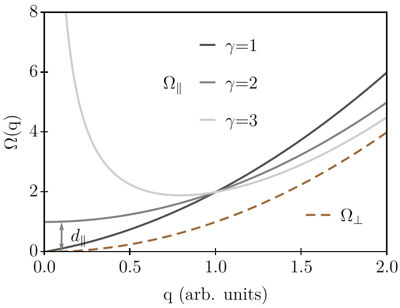
Figure 4: Dispersion of the longitudinal (solid) and transverse (dashed) modes of 2D WCs. Here, we have set $c_{a}=1=d_{\parallel}$. $\gamma=1$ corresponds to the long-range Coulomb interaction. With increasing $\gamma$, the interaction becomes increasingly short-range. For $\gamma=2$, as can be seen from Eq. (16), a gap of size $d_{\parallel}$ appears in the longitudinal mode. With further increase in $\gamma$, this gap diverges.

IV Gaussian Variational Minimization

In this section, we treat the effective Hamiltonian obtained in the previous section using the Gaussian variational method (GVM) developed in Refs. Giamarchi and Le Doussal (1995, 1997); Fukuyama and Lee (1978). This allows us to obtain the dispersion of the vibrational modes of the GWC and the associated pinning gap arising from the interaction between the Wigner lattice and the moiré lattice. Motivated by the experiments, we assume the GWCs to be weakly coupled to the moiré lattice. This allows us to treat the vibrations of the localized particles as harmonic fluctuations. This is formalized by the GVM as follows. Consider a Hamiltonian $H=\frac{1}{2}\int_{q}u(q)\,\Omega(q)u(-q)+H^{\prime}$, where the kernel $\Omega(q)$ is known a priori and $H^{\prime}$ can contain non-linear or polynomial terms in the field $u(q)$. For a vector field $\boldsymbol{u}(\boldsymbol{q})$, this kernel becomes a matrix. The goal is to approximate the Hamiltonian $H$ by the following quadratic form,

$$H_{0}=\frac{1}{2}\int_{q}u(q)\,{\mathcal{G}}^{-1}(q)\,u(-q)\,.$$ (17)

The optimal function $\mathcal{G}(q)$ is then obtained by minimizing the variational free energy of the theory $H$, $F_{\rm var}=F_{0}+\langle H-H_{0}\rangle_{0}$ where $\langle\mathcal{..}\rangle_{0}$ is the expectation value evaluated with $H_{0}$ with respect to $\mathcal{G}(q)$. In App. C we provide a pedagogical discussion on using this GVM method for the simple case of a Sine-Gordon (SG) interaction as the hamiltonian in (16) closely resembles the SG problem.

IV.1 Applying GVM to GWC

We use the GVM to obtain the gap opened by the moiré lattice. Since the displacement is a two component field we have both $\Omega_{\mkern 3.0mu\vphantom{\perp}\vrule depth=0.0pt\mkern 2.0mu\vrule depth=0.0pt\mkern 3.0mu}(\boldsymbol{q})$ and $\Omega_{\perp}(\boldsymbol{q})$. The variational free energy becomes

$$F_{\mathrm{var}}=\frac{T}{2}\int_{q}\sum_{a=\parallel,\perp}\Big{\{}\Omega_{a}(\boldsymbol{q})\mathcal{G}_{a}(\boldsymbol{q})-\log[T\mathcal{G}_{a}(\boldsymbol{q})]\Big{\}}-$$

$$\sum_{l,m}V_{m}\,\delta\left(\boldsymbol{K}_{l}-\boldsymbol{G}_{m}\right)\,\exp\left[-\frac{T}{2}\sum_{b=\parallel,\perp}K_{l,b}^{2}\,\int_{\boldsymbol{q}}\mathcal{G}_{b}(\boldsymbol{q})\right].$$ (18)

Note that in the absence of a magnetic field there is no admixture of the longitudinal and transverse modes.

The Green function that minimizes the free energy in Eq. (IV.1) can be approximated by $\mathcal{G}^{(0)}_{a}(\boldsymbol{q})\simeq\frac{1}{\Omega_{a}(\boldsymbol{q})+\Delta_{a}}$, where the gaps $\Delta_{a}$ satisfy the following self-consistent equations (SCE)

$$\Delta_{a}=\sum_{m\in\mathcal{M}}V_{m}^{\phantom{2}}G_{m,a}^{2}\exp\left(-\frac{T}{2}\int_{\boldsymbol{q}}\sum_{b=\perp,{\mkern 3.0mu\vphantom{\perp}\vrule depth=0.0pt\mkern 2.0mu\vrule depth=0.0pt\mkern 3.0mu}}\frac{G_{m,b}^{2}}{\Omega_{b}(\boldsymbol{q})+\Delta_{b}}\right).$$ (19)

Here $a$ is not in the Cartesian basis but in the orthonormal basis discussed in Eq. (13). Though at first glance Eq. (19) seems independent of $\boldsymbol{K}_{l}$ (or $\lambda_{\mathrm{w}}$), we note that the conservation of momentum imposed through the delta function in Eq. (IV.1), restricts the set of $\boldsymbol{G}_{m}$ to those satisfying $r\boldsymbol{G}_{1}=s\boldsymbol{K}_{1}$. The set of such restricted (momentum conserving) values of $\boldsymbol{G}_{m}$ is denoted by $\mathcal{M}$. For instance, for the WC at $1/3$-filling, since, as explained previously, $r=1$, $\mathcal{M}$ is trivially the first MBZ. After integrating, we find that the gap equations take the form

$$\Delta_{a}\simeq \sum_{m\in\mathcal{M}}V_{m}^{\phantom{2}}G_{m,a}^{2}\left(\frac{\Delta_{\perp}}{c_{\perp}\Lambda^{2}}\right)^{\frac{TG_{m,\perp}^{2}}{8\pi c_{\perp}}}\left(\frac{\Delta_{\mkern 3.0mu\vphantom{\perp}\vrule depth=0.0pt\mkern 2.0mu\vrule depth=0.0pt\mkern 3.0mu}}{c_{\mkern 3.0mu\vphantom{\perp}\vrule depth=0.0pt\mkern 2.0mu\vrule depth=0.0pt\mkern 3.0mu}\Lambda^{2}}\right)^{\frac{TG_{m,{\mkern 3.0mu\vphantom{\perp}\vrule depth=0.0pt\mkern 2.0mu\vrule depth=0.0pt\mkern 3.0mu}}^{2}}{8\pi c_{\mkern 3.0mu\vphantom{\perp}\vrule depth=0.0pt\mkern 2.0mu\vrule depth=0.0pt\mkern 3.0mu}}}$$

$$\times\exp\left[{\frac{TG_{m,{\mkern 3.0mu\vphantom{\perp}\vrule depth=0.0pt\mkern 2.0mu\vrule depth=0.0pt\mkern 3.0mu}}^{2}}{8\pi c_{\mkern 3.0mu\vphantom{\perp}\vrule depth=0.0pt\mkern 2.0mu\vrule depth=0.0pt\mkern 3.0mu}}\tilde{\Delta}_{\mkern 3.0mu\vphantom{\perp}\vrule depth=0.0pt\mkern 2.0mu\vrule depth=0.0pt\mkern 3.0mu}\left(\pi+2\tan^{-1}\tilde{\Delta}_{\mkern 3.0mu\vphantom{\perp}\vrule depth=0.0pt\mkern 2.0mu\vrule depth=0.0pt\mkern 3.0mu}\right)}\right].$$ (20)

Here, ${d_{\mkern 3.0mu\vphantom{\perp}\vrule depth=0.0pt\mkern 2.0mu\vrule depth=0.0pt\mkern 3.0mu}}/{\sqrt{4c_{\mkern 3.0mu\vphantom{\perp}\vrule depth=0.0pt\mkern 2.0mu\vrule depth=0.0pt\mkern 3.0mu}\Delta_{\mkern 3.0mu\vphantom{\perp}\vrule depth=0.0pt\mkern 2.0mu\vrule depth=0.0pt\mkern 3.0mu}-d_{\mkern 3.0mu\vphantom{\perp}\vrule depth=0.0pt\mkern 2.0mu\vrule depth=0.0pt\mkern 3.0mu}^{2}}}\equiv\tilde{\Delta}_{\mkern 3.0mu\vphantom{\perp}\vrule depth=0.0pt\mkern 2.0mu\vrule depth=0.0pt\mkern 3.0mu}$ and $\Lambda$ is a UV cutoff for the momentum space integration. The zero temperature limit for the gap above is $\sum_{m\in\mathcal{M}}V_{m}^{\phantom{2}}G_{m,a}^{2}\equiv\Delta_{a}^{0}$. And, a low temperature expansion is obtained to be

$$\Delta_{\perp}=A_{\perp}+B_{\perp}\log\Delta_{\perp};$$

$$A_{\perp}=\Delta_{\perp}^{0}+T\sum_{m\in\mathcal{M}}V_{m}^{\phantom{2}}G_{m,\perp}^{2}\left[D_{m}^{{\mkern 3.0mu\vphantom{\perp}\vrule depth=0.0pt\mkern 2.0mu\vrule depth=0.0pt\mkern 3.0mu}}-\frac{G_{m,\perp}^{2}}{8\pi c_{\perp}}\log{c_{\perp}\Lambda^{2}}\right],$$

$$D_{m}^{{\mkern 3.0mu\vphantom{\perp}\vrule depth=0.0pt\mkern 2.0mu\vrule depth=0.0pt\mkern 3.0mu}}=\frac{G_{m,{\mkern 3.0mu\vphantom{\perp}\vrule depth=0.0pt\mkern 2.0mu\vrule depth=0.0pt\mkern 3.0mu}}^{2}}{8\pi c_{\mkern 3.0mu\vphantom{\perp}\vrule depth=0.0pt\mkern 2.0mu\vrule depth=0.0pt\mkern 3.0mu}}\log\frac{\Delta_{\mkern 3.0mu\vphantom{\perp}\vrule depth=0.0pt\mkern 2.0mu\vrule depth=0.0pt\mkern 3.0mu}}{c_{\mkern 3.0mu\vphantom{\perp}\vrule depth=0.0pt\mkern 2.0mu\vrule depth=0.0pt\mkern 3.0mu}\Lambda^{2}}+\frac{G_{m,{\mkern 3.0mu\vphantom{\perp}\vrule depth=0.0pt\mkern 2.0mu\vrule depth=0.0pt\mkern 3.0mu}}^{2}}{8\pi c_{\mkern 3.0mu\vphantom{\perp}\vrule depth=0.0pt\mkern 2.0mu\vrule depth=0.0pt\mkern 3.0mu}}\tilde{\Delta}_{\mkern 3.0mu\vphantom{\perp}\vrule depth=0.0pt\mkern 2.0mu\vrule depth=0.0pt\mkern 3.0mu}\left(\pi+2\tan^{-1}\tilde{\Delta}_{\mkern 3.0mu\vphantom{\perp}\vrule depth=0.0pt\mkern 2.0mu\vrule depth=0.0pt\mkern 3.0mu}\right),$$

$$B_{\perp}=T\sum_{m\in\mathcal{M}}V_{m}^{\phantom{2}}\frac{G_{m,\perp}^{4}}{8\pi c_{\perp}}.$$ (21)

Here $A_{\perp}$ is dependent on $\Delta_{{\mkern 3.0mu\vphantom{\perp}\vrule depth=0.0pt\mkern 2.0mu\vrule depth=0.0pt\mkern 3.0mu}}$, and $B_{\perp}$ is a geometric constant. From this, we obtain a closed-form expression for $\Delta_{\perp}$ in terms of $\Delta_{{\mkern 3.0mu\vphantom{\perp}\vrule depth=0.0pt\mkern 2.0mu\vrule depth=0.0pt\mkern 3.0mu}}$. By bringing the above equation to the form $we^{w}=z$, we obtain the solution $w=W_{k}(z)$, where $W_{k}(z)$ is the (multivalued) Lambert $W$ function with its branch indexed by the integer $k$. In fact, when $w<0$ (for us, $w=-\Delta_{\perp}/B_{\perp}$), the solution has two branches, $W_{0}(z)$ and $W_{-1}(z)$. We will drop the latter solution since it is not a regular function at $\Delta_{\perp}=0$. Therefore,

$$\Delta_{\perp}=-B_{\perp}W_{0}\left(-\frac{e^{-A_{\perp}/B_{\perp}}}{B_{\perp}}\right).$$ (22)

This is the explicit dependence of $\Delta_{\perp}$ on $\Delta_{{\mkern 3.0mu\vphantom{\perp}\vrule depth=0.0pt\mkern 2.0mu\vrule depth=0.0pt\mkern 3.0mu}}$ (through $A_{\perp}$ only). Similarly, an SCE for the $\Delta_{{\mkern 3.0mu\vphantom{\perp}\vrule depth=0.0pt\mkern 2.0mu\vrule depth=0.0pt\mkern 3.0mu}}$ component is

$$\Delta_{{\mkern 3.0mu\vphantom{\perp}\vrule depth=0.0pt\mkern 2.0mu\vrule depth=0.0pt\mkern 3.0mu}}^{\phantom{0}}=\Delta_{{\mkern 3.0mu\vphantom{\perp}\vrule depth=0.0pt\mkern 2.0mu\vrule depth=0.0pt\mkern 3.0mu}}^{0}+T\sum_{m\in\mathcal{M}}V_{m}^{\phantom{2}}G_{m,{\mkern 3.0mu\vphantom{\perp}\vrule depth=0.0pt\mkern 2.0mu\vrule depth=0.0pt\mkern 3.0mu}}^{2}\frac{G_{m,\perp}^{2}}{8\pi c_{\perp}}\log\frac{\Delta_{\perp}}{c_{\perp}\Lambda^{2}},$$ (23)

where $\Delta_{\perp}$ is given by Eq. (22). In the next subsection we discuss the solutions obtained here, especially in conjunction with the recent experiments.

IV.2 Discussions

Note that the last term in Eq. (IV.1) is an artifact of the long-range interaction which vanishes if $d_{\parallel}=0$. This term, which is the compression term, purely accounts for the elastic contribution to the gap. For $d_{{\mkern 3.0mu\vphantom{\perp}\vrule depth=0.0pt\mkern 2.0mu\vrule depth=0.0pt\mkern 3.0mu}}=0$, the gap equation is equivalent to the vector SG potential, see Eq. (C15).

Secondly, since $\Lambda$ appears in the denominator of Eq. (IV.1), the gap vanishes for temperatures larger than a characteristic temperature, $\mathrm{min}\left(\frac{8\pi c_{\mkern 3.0mu\vphantom{\perp}\vrule depth=0.0pt\mkern 2.0mu\vrule depth=0.0pt\mkern 3.0mu}}{G_{{\mkern 3.0mu\vphantom{\perp}\vrule depth=0.0pt\mkern 2.0mu\vrule depth=0.0pt\mkern 3.0mu}}^{2}},\frac{8\pi c_{\perp}}{G_{\perp}^{2}}\right)\equiv T_{\ast}$. This is a feature of the equivalence of the effective interaction Hamiltonian to that with the SG potential, see discussions in the App. C. The analysis is valid only if $T_{\ast}$ is much smaller than the melting temperature (such as $T_{\rm L}$) of a GWC. Note that since $T_{\ast}\sim{c_{a}}{\lambda^{2}_{\rm w}}$, this temperature scale can be controlled by means of the twist angle.

The pinning frequency is related to the zero temperature gap as Fukuyama and Lee (1978) $\omega_{p}^{a}=\sqrt{\Delta^{0}_{a}/\rho_{0}}$. Notably, since the pinning frequency scales with the size of the WBZ, $\omega_{p}^{a}\propto G_{a}$, it becomes increasingly difficult to de-pin a WC of smaller unit cell. This is since a WC with large unit cell (or small $\boldsymbol{G}$) will be loosely bound compared to one with smaller unit cell (as the particles are more tightly packed). Therefore, the former can be easily de-pinned by an external electric field. Similarly, for a deeper moiré potential the pinning frequency increases ($\omega_{p}^{a}\propto\tilde{V}^{1/2}$) since the particles get tightly bound to the potential minima. Introduction of a spacer layer can further modulate this frequency. Geometrical factors aside, the pinning gap thus becomes $\mathcal{O}(\lesssim\rm meV)$. With increasing temperature, as seen in Eq. (21), this gap softens as the increasing thermal fluctuation facilitates de-pinning. The extent to which this gap decreases depends on various coefficients appearing in Eq. (21). Most notably, via the elastic constants, $c_{\alpha}$, the logarithm term has a coefficient that is directly proportional to the dielectric term. Thus, the larger the screening, the smaller the pinning gap. Therefore, although the geometrical constants associated with various HoM or HeM TMDs may not affect the pinning gap of a GWC, the dielectric constant can however alter the physics. This gap translates into determining which state is a stronger insulator.

V Conclusion

We have addressed the feasibility of realizing Wigner crystals in a host of HoM and HeM systems. Note however, that our results are based on estimated material parameters of the TMD moiré materials. Corrections to these results might arise principally from three sources. The first is from the full band structure of the TMD heterostructures Padhi and Phillips (2019). Second, a material correction arising from twist-angle inhomogeneity across a sample Uri et al. (2020); Padhi et al. (2020) which may cause additional pinning or de-pinning of the WC could also affect the physics. Similar effects may also arise from atomic relaxations Nam and Koshino (2017); Uchida et al. (2014). Third, the presence or absence of a spacer layer Shimazaki et al. (2020a), such as a monolayer hBN, may also affect the correlation energy, thereby affecting Wigner crystallization. A first principles calculation of the elastic coefficients of the GWC is also important to obtain good qualitative and quantitative estimates for the pinning gap and the phonon spectrum. All of these aspects merit further studies as this will help narrow the density and temperature regimes where WC is feasible.

Due to the presence of a pinning gap, transport measurements to confirm the existence of WC states can be misleading as there can be many other kinds of insulating states with similar transport characteristics. Although observation of such states at fractional occupancy increases their likelihood of being Wigner states, especially for those observed at incommensurate fillings, however, the possibility of other density ordered states cannot be ruled out, particularly for commensurate fractional occupancies. Devising smoking gun evidence for various density ordered states may be an interesting task for theorists and experimentalists alike.

As was mentioned before, once a system meets the material constraints to realize a GWC, there exists a plethora of crystalline states below the filling fraction $\nu^{\rm max}$. These states constitute a devil’s staircase and have a rich physics of commensurate-incommensurate transitions Bak (1982); Aubry (1983); Pokrovsky and Virosztek (1983). Due to various stability criteria, only a few such states might display clear experimental signatures. However, with careful analysis or improvements in experimental conditions, one may gain insight into the other states as well. In fact, a theoretical framework to understand these commensurate-incommensurate transitions in presence of an underlying lattice is an interesting theoretical task and is left for future work.

B.P. and P.W.P. thank the NSF under grant DMR19-19143 for partial funding of this project.

Appendix

Appendix A Harmonic Expansion of Density

Following Giamarchi and Le Doussal (1995), we derive the elastic limit of the density written in Eq. (5). A continuum limit can be easily obtained if we treat the equilibrium GWC configuration, $\boldsymbol{R}_{i}^{0}=\boldsymbol{R}_{i}-\boldsymbol{u}(\boldsymbol{R}_{i}^{0})$, as a slowly varying smooth vector field, $\boldsymbol{\varphi}(\boldsymbol{x})$, over the position of the particles

$$\boldsymbol{\varphi}(\boldsymbol{x})=\boldsymbol{x}-\boldsymbol{u}\left(\boldsymbol{\varphi}(\boldsymbol{x})\right)\,.$$ (A1)

Clearly a solution of $\boldsymbol{\varphi}(\boldsymbol{x})$ is given by, $\boldsymbol{\varphi}(\boldsymbol{R}_{i})=\boldsymbol{\varphi}\left(\boldsymbol{R}_{i}^{0}+\boldsymbol{u}(\boldsymbol{R}_{i}^{0})\right)=\boldsymbol{R}_{i}^{0}$. Using the above equality we can rewrite the density in terms of this new field as

$$\rho(\boldsymbol{x})= \sum_{i}\delta^{(2)}\left[\boldsymbol{R}_{i}-\boldsymbol{\varphi}(\boldsymbol{x})-\boldsymbol{u}(\boldsymbol{\varphi}(\boldsymbol{x}))\right]$$ (A2a)

$$\simeq \det[\boldsymbol{\partial}_{\alpha}\boldsymbol{\varphi}_{\beta}(\boldsymbol{x})]\sum_{i}\delta^{(2)}\left(\boldsymbol{R}_{i}-\boldsymbol{\varphi}(\boldsymbol{x})\right)$$ (A2b)

$$= \det[\boldsymbol{\partial}_{\alpha}\boldsymbol{\varphi}_{\beta}(\boldsymbol{x})]\int\frac{d\boldsymbol{q}}{(2\pi)^{2}}\rho_{0}(\boldsymbol{q})e^{i\boldsymbol{q}\cdot\boldsymbol{\varphi}(\boldsymbol{x})}\,.$$ (A2c)

The first simplification was done using the elastic limit, $\boldsymbol{\partial}_{\alpha}\boldsymbol{u}_{\beta}\ll 1$. In the last line, we have used the integral representation of the delta function. In the presence of an undeformed GWC, we can introduce its reciprocal vectors, $e^{i\boldsymbol{K}_{l}\cdot\boldsymbol{R}_{i}}=1$, to write

$$\rho_{0}(\boldsymbol{q})=\sum_{i}e^{i\boldsymbol{q}\cdot\boldsymbol{R}_{i}}=\rho_{0}(2\pi)^{2}\sum_{l}\delta^{(2)}(\boldsymbol{q}-\boldsymbol{K}_{l})\,.$$ (A3)

Here $\rho_{0}$ is the average number density. Introducing the above simplification in Eq. (A2c) and using Eq. (A1), we obtain

$$\rho(\boldsymbol{x})= \rho_{0}\det[\boldsymbol{\partial}_{\alpha}\boldsymbol{\varphi}_{\beta}(\boldsymbol{x})]\sum_{l}e^{i\boldsymbol{K}_{l}\cdot\boldsymbol{\varphi}(\boldsymbol{x})}$$

$$= \rho_{0}\det[1-\boldsymbol{\partial}_{\alpha}\boldsymbol{u}_{\beta}\left(\boldsymbol{\varphi}(\boldsymbol{x})\right)]\sum_{l}e^{i\boldsymbol{K}_{l}\cdot\left[\boldsymbol{x}-\boldsymbol{u}(\boldsymbol{\varphi}(\boldsymbol{x}))\right]}$$

$$\simeq \rho_{0}-\rho_{0}\boldsymbol{\nabla}\cdot\boldsymbol{u}(\boldsymbol{x})+\rho_{0}\sum_{l}e^{i\boldsymbol{K}_{l}\cdot\left[\boldsymbol{x}-\boldsymbol{u}(\boldsymbol{x})\right]}\,.$$ (A4)

We again used the elastic limit by first Taylor-expanding the determinant operator, $\det$, and then substituting $\boldsymbol{u}(\boldsymbol{\varphi}(\boldsymbol{x}))\approx\boldsymbol{u}(\boldsymbol{x})$ which works for $\boldsymbol{x}$ close to the equilibrium position and in the elastic limit. This leads us to Eq. (5). Note there is complete decoupling between the gradient term and the terms with $\boldsymbol{K}_{l}$. This occurs because $\boldsymbol{u}(\boldsymbol{x})$ has negligible Fourier components outside the WBZ.

Appendix B Elastic Interaction Hamiltonian

In this Appendix, we clarify the derivation of Eq. (15). First, we Fourier transform the second part of Eq. (III.2),

$$H_{\mathrm{e}\text{--}\mathrm{e}}^{(2)} =\frac{1}{2}\sum_{l}\int_{\boldsymbol{x},\boldsymbol{x}^{\prime}}U(\boldsymbol{x}-\boldsymbol{x}^{\prime})e^{i\boldsymbol{K}_{l}\cdot(\boldsymbol{x}-\boldsymbol{x}^{\prime})}K_{l,\alpha}K_{l,\beta}\,\times$$

$$\int_{\boldsymbol{q},\boldsymbol{q}^{\prime}}u_{\alpha}(\boldsymbol{q})\,u_{\beta}(\boldsymbol{q}^{\prime})\,\left(e^{i\boldsymbol{q}\cdot\boldsymbol{x}}-e^{i\boldsymbol{q}\cdot\boldsymbol{x}^{\prime}}\right)\left(e^{i\boldsymbol{q}^{\prime}\cdot\boldsymbol{x}}-e^{i\boldsymbol{q}^{\prime}\cdot\boldsymbol{x}^{\prime}}\right).$$ (B5)

In order to simplify it further, we introduce the center of mass coordinate, $2\boldsymbol{X}=\boldsymbol{x}+\boldsymbol{x}^{\prime}$ and the relative coordinate $2\boldsymbol{\delta}=\boldsymbol{x}-\boldsymbol{x}^{\prime}$ to obtain

$$H_{\mathrm{e}\text{--}\mathrm{e}}^{(2)}= \sum_{l}K_{l,\alpha}K_{l,\beta}\int_{\boldsymbol{q}}u_{\alpha}(\boldsymbol{q})u_{\beta}(-\boldsymbol{q})\,\times$$

$$\int_{\boldsymbol{\delta}}d\boldsymbol{\delta}\,U(\boldsymbol{\delta})\left[1-\cos(\boldsymbol{q}\cdot\boldsymbol{\delta})\right]e^{i\boldsymbol{K}_{l}\cdot\boldsymbol{\delta}}.$$ (B6)

In coming to this line, we have also integrated out $\boldsymbol{q}^{\prime}$, which introduced a delta function, $\delta^{(2)}(\boldsymbol{q}+\boldsymbol{q}^{\prime})$. Next, we perform the last integration for a generic potential of the form, $U(\boldsymbol{x})=e^{2}/\epsilon|\boldsymbol{x}|^{\gamma}$. One can obtain the long-range Coulomb potential by setting $\gamma=1$, and with increasing $\gamma$ the potential becomes increasingly short-range. For such a $U(\boldsymbol{\delta})$ we find that

$$H_{\mathrm{e}\text{--}\mathrm{e}}^{(2)}= \sum_{l}K_{l,\alpha}K_{l,\beta}\int_{\boldsymbol{q}}u_{\alpha}(\boldsymbol{q})u_{\beta}(-\boldsymbol{q})\,\times$$

$$\frac{e^{2}}{\epsilon}\left(\frac{2}{|\boldsymbol{K}_{l}|^{\gamma}}-\frac{1}{|\boldsymbol{K}_{l}-\boldsymbol{q}|^{\gamma}}-\frac{1}{|\boldsymbol{K}_{l}+\boldsymbol{q}|^{\gamma}}\right).$$ (B7)

For further simplification, we confine our discussion to the low-energy limit. This allows us to Taylor-expand the last term in Eq. (B7) for the limit $|\boldsymbol{q}|\ll|\boldsymbol{K}_{l}|$. The first term in this expansion, which is linear in $\boldsymbol{q}$, vanishes because it involves integrating over a $\cos\theta_{l}$ term. Here, $\theta_{l}$ are the angles between the $\boldsymbol{q}$ vector and $\boldsymbol{K}_{l}$. Therefore, retaining up to the $\mathcal{O}(q^{2})$ term we obtain,

$$H_{\mathrm{e}\text{--}\mathrm{e}}^{(2)}\simeq\gamma\frac{e^{2}}{\epsilon}\, \sum_{l}\frac{K_{l,\alpha}K_{l,\beta}}{|\boldsymbol{K}_{l}|^{2+\gamma}}\int_{\boldsymbol{q}}q^{2}u_{\alpha}(\boldsymbol{q})u_{\beta}(-\boldsymbol{q})\,\times$$

$$\left[(2+\gamma)\cos^{2}\theta_{l}-1\right].$$ (B8)

Note that unlike the long-distance term, $H_{\mathrm{e}\text{--}\mathrm{e}}^{(1)}$ in Eq. (14), the leading dispersion corresponding to $H_{\mathrm{e}\text{--}\mathrm{e}}^{(2)}$ remains quadratic regardless of the choice of $\gamma$.

$$H_{\mathrm{e}\text{--}\mathrm{e}}^{(2)}=\int_{\boldsymbol{q}}c_{\mkern 3.0mu\vphantom{\perp}\vrule depth=0.0pt\mkern 2.0mu\vrule depth=0.0pt\mkern 3.0mu}q^{2}u_{\mkern 3.0mu\vphantom{\perp}\vrule depth=0.0pt\mkern 2.0mu\vrule depth=0.0pt\mkern 3.0mu}(\boldsymbol{q})u_{\mkern 3.0mu\vphantom{\perp}\vrule depth=0.0pt\mkern 2.0mu\vrule depth=0.0pt\mkern 3.0mu}(-\boldsymbol{q})+c_{\perp}q^{2}u_{\perp}(\boldsymbol{q})u_{\perp}(-\boldsymbol{q}).$$ (B9)

Appendix C GVM for Sine-Gordon Potential

In this Appendix, we demonstrate the GVM method discussed in the main text for a Sine-Gordon (SG) potential,

$$H=\frac{1}{2}c\int dx\,\left[\nabla\phi(x)\right]^{2}-g\int dx\cos[2\phi(x)].$$ (C10)

Here $c$ and $g$ are free parameters. Using the simplifications discussed in the main text [and using $\Omega(q)=cq^{2}$], we obtain the variational free energy to be

$$F_{\mathrm{var}} =-\frac{T}{2}\int_{q}\log[T\mathcal{G}(q)]+\frac{T}{2}\int_{q}cq^{2}\mathcal{G}(q)-$$

$$g\left.\exp\left[\frac{T}{2}\int_{q}\mathcal{G}(q)\frac{\partial^{2}}{\partial\phi^{2}}\right]\int dx\cos(2\phi)\right\rvert_{\phi=0}.$$ (C11)

Further simplifications of the last term leads us to

$$F_{\mathrm{var}}= -\frac{T}{2}\int_{q}\log[T\mathcal{G}(q)]+\frac{T}{2}\int_{q}cq^{2}\mathcal{G}(q)-ge^{-2\int_{q}T\mathcal{G}(q)}.$$ (C12)

In these equations, we fixed the sample area to $\int dx=1$. The saddle point solution of the above free energy is

$$\mathcal{G}^{-1}=cq^{2}+4ge^{-2\int_{q}T\mathcal{G}(q)}.$$ (C13)

We now set $\mathcal{G}^{-1}(q)=cq^{2}+m$ and solve $m$ self-consistently,

$$m=4ge^{-2T\int_{q}^{\Lambda}\frac{1}{cq^{2}+m}}\simeq 4g\left(\frac{m}{c\Lambda^{2}}\right)^{T/2\pi c}.$$ (C14)

Here, $\Lambda$ is a UV cutoff in the momentum-space. A notable feature of this solution is that beyond a certain temperature maximum, $T>2\pi c$, the SG mass must vanish simply due to the presence of the cutoff in the denominator above. Such a maximal temperature will also appear in our discussion in Sec. IV.2. Additionally, from Eq. (C14) one can also deduce the scaling behavior of the mass, $m\sim g^{1/(1-\tau)}$, where $\tau=T/2\pi c$.

Pertaining to our discussion of GVM in the context of GWC, we extend the previous solutions for a SG potential to an $n$-component vector SG system. The interaction term here becomes $H^{\prime}\sim\int dx\cos(\sum_{n}p_{n}\phi_{n})$. The kernel corresponding to the field $\phi_{n}$ is $c_{n}q^{2}$. As before, we obtain the variational free energy

$$F_{\mathrm{var}}= -\frac{T}{2}\sum_{n}\int_{q}\left\{\log[T\mathcal{G}_{n}(q)]-c_{n}q^{2}\mathcal{G}_{n}(q)\right\}$$

$$-ge^{-\frac{T}{2}\sum_{n}a_{n}^{2}\int_{q}\mathcal{G}(q)}.$$ (C15a)

Since, due to the vanishing average of cosine functions, there are no cross terms such as $$\cos\phi_{m}\cos\phi_{n} m\neq n n=1 a_{n}=2$$ (with ), the saddle-point equation (setting and goes back to the original case)

$$\mathcal{G}_{n}^{-1} =c_{n}q^{2}+ga_{n}^{2}e^{-\frac{T}{2}\sum_{n}a^{2}_{n}\int_{q}\mathcal{G}_{n}(q)},$$ (C15b)

$$\therefore\quad m_{n} =ga_{n}^{2}\exp\left[-\sum_{n}\frac{Ta^{2}_{n}}{8\pi c_{n}}\log\left(\frac{c_{n}\Lambda^{2}}{m_{n}}\right)\right].$$ (C15c)

We can solve this SCE exactly and, in this case as well, there exists a similar temperature window where gap vanishes, ${Ta^{2}_{n}}/{8\pi c_{n}}\equiv\tau_{n}>1$. And, like before, the scaling of $m_{n}$ with the coupling constant becomes, $m_{n}\propto g^{\left(1-\sum_{n}\tau_{n}\right)^{-1}}$. These solutions are not exactly transferable for our discussions in the main text since there the kernel has a $d_{{\mkern 3.0mu\vphantom{\perp}\vrule depth=0.0pt\mkern 2.0mu\vrule depth=0.0pt\mkern 3.0mu}}q^{2-\gamma}$ part. See Sec. IV.2 for the case when $d_{{\mkern 3.0mu\vphantom{\perp}\vrule depth=0.0pt\mkern 2.0mu\vrule depth=0.0pt\mkern 3.0mu}}=0$, where the above results are perfectly applicable.

References

- Wigner (1934) E. Wigner, “On the interaction of electrons in metals,” Phys. Rev. 46, 1002–1011 (1934).
- Grimes and Adams (1979) C. C. Grimes and G. Adams, “Evidence for a liquid-to-crystal phase transition in a classical, two-dimensional sheet of electrons,” Phys. Rev. Lett. 42, 795–798 (1979).
- Monarkhaa and V. E. Syvokon (2012) Y. P. Monarkhaa and V. E. V. E. Syvokon, “A two-dimensional wigner crystal (review article),” Low Temperature Physics 38, 1067 (2012).
- Cao et al. (2018a) Y. Cao, V. Fatemi, A. Demir, S. Fang, S. L. Tomarken, J. Y. Luo, J. D. Sanchez-Yamagishi, K. Watanabe, T. Taniguchi, E. Kaxiras, R. C. Ashoori, and P. Jarillo-Herrero, “Correlated insulator behaviour at half-filling in magic-angle graphene superlattices,” Nature 556, 80 (2018a).
- Cao et al. (2018b) Y. Cao, V. Fatemi, S. Fang, K. Watanabe, T. Taniguchi, E. Kaxiras, and P. Jarillo-Herrero, “Unconventional superconductivity in magic-angle graphene superlattices,” Nature 556, 43 (2018b).
- Yankowitz et al. (2019) M. Yankowitz, S. Chen, H. Polshyn, Y. Zhang, K. Watanabe, T. Taniguchi, D. Graf, A. F. Young, and C. R. Dean, “Tuning superconductivity in twisted bilayer graphene,” Science (2019), 10.1126/science.aav1910.
- Lu et al. (2019) X. Lu, P. Stepanov, W. Yang, M. Xie, M. A. Aamir, I. Das, C. Urgell, K. Watanabe, T. Taniguchi, G. Zhang, A. Bachtold, A. H. MacDonald, and D. K. Efetov, “Superconductors, orbital magnets and correlated states in magic-angle bilayer graphene,” Nature 574, 653–657 (2019).
- Kerelsky et al. (2018) A. Kerelsky, L. McGilly, D. M. Kennes, L. Xian, M. Yankowitz, S. Chen, K. Watanabe, T. Taniguchi, J. Hone, C. Dean, A. Rubio, and A. N. Pasupathy, “Magic Angle Spectroscopy,” arXiv e-prints , arXiv:1812.08776 (2018), arXiv:1812.08776 [cond-mat.mes-hall] .
- Choi et al. (2019) Y. Choi, J. Kemmer, Y. Peng, A. Thomson, H. Arora, R. Polski, Y. Zhang, H. Ren, J. Alicea, G. Refael, F. von Oppen, K. Watanabe, T. Taniguchi, and S. Nadj-Perge, “Imaging Electronic Correlations in Twisted Bilayer Graphene near the Magic Angle,” arXiv e-prints , arXiv:1901.02997 (2019), arXiv:1901.02997 [cond-mat.mes-hall] .
- Wong et al. (2020) D. Wong, K. P. Nuckolls, M. Oh, B. Lian, Y. Xie, S. Jeon, K. Watanabe, T. Taniguchi, B. A. Bernevig, and A. Yazdani, “Cascade of electronic transitions in magic-angle twisted bilayer graphene,” Nature 582, 198–202 (2020).
- Zondiner et al. (2020) U. Zondiner, A. Rozen, D. Rodan-Legrain, Y. Cao, R. Queiroz, T. Taniguchi, K. Watanabe, Y. Oreg, F. von Oppen, A. Stern, and et al., “Cascade of phase transitions and dirac revivals in magic-angle graphene,” Nature 582, 203–208 (2020).
- Stepanov et al. (2019) P. Stepanov, I. Das, X. Lu, A. Fahimniya, K. Watanabe, T. Taniguchi, F. H. L. Koppens, J. Lischner, L. Levitov, and D. K. Efetov, “The interplay of insulating and superconducting orders in magic-angle graphene bilayers,” (2019), arXiv:1911.09198 [cond-mat.supr-con] .
- Regan et al. (2020) E. C. Regan, D. Wang, C. Jin, M. I. Bakti Utama, B. Gao, X. Wei, S. Zhao, W. Zhao, Z. Zhang, K. Yumigeta, and et al., “Mott and generalized Wigner crystal states in WSe2/WS2 moiré superlattices,” Nature 579, 359–363 (2020).
- Xu et al. (2020) Y. Xu, S. Liu, D. A. Rhodes, K. Watanabe, T. Taniguchi, J. Hone, V. Elser, K. F. Mak, and J. Shan, “Abundance of correlated insulating states at fractional fillings of wse2/ws2 moiré superlattices,” (2020), arXiv:2007.11128 [cond-mat.str-el] .
- Jin et al. (2020) C. Jin, Z. Tao, T. Li, Y. Xu, Y. Tang, J. Zhu, S. Liu, K. Watanabe, T. Taniguchi, J. C. Hone, L. Fu, J. Shan, and K. F. Mak, “Stripe phases in wse2/ws2 moiré superlattices,” (2020), arXiv:2007.12068 [cond-mat.mes-hall] .
- Shimazaki et al. (2020a) Y. Shimazaki, I. Schwartz, K. Watanabe, T. Taniguchi, M. Kroner, and A. Imamoğlu, “Strongly correlated electrons and hybrid excitons in a moiré heterostructure,” Nature 580, 472–477 (2020a).
- Tang et al. (2020) Y. Tang, L. Li, T. Li, Y. Xu, S. Liu, K. Barmak, K. Watanabe, T. Taniguchi, A. H. MacDonald, J. Shan, et al., “Simulation of hubbard model physics in wse 2/ws 2 moiré superlattices,” Nature 579, 353–358 (2020).
- Wu et al. (2018) F. Wu, T. Lovorn, E. Tutuc, and A. H. MacDonald, “Hubbard model physics in transition metal dichalcogenide moiré bands,” Phys. Rev. Lett. 121, 026402 (2018).
- Wu et al. (2019) F. Wu, T. Lovorn, E. Tutuc, I. Martin, and A. H. MacDonald, “Topological insulators in twisted transition metal dichalcogenide homobilayers,” Phys. Rev. Lett. 122, 086402 (2019).
- Bistritzer and MacDonald (2011) R. Bistritzer and A. H. MacDonald, “Moiré bands in twisted double-layer graphene,” Proceedings of the National Academy of Sciences 108, 12233–12237 (2011).
- Wang et al. (2019) L. Wang, E.-M. Shih, A. Ghiotto, L. Xian, D. A. Rhodes, C. Tan, M. Claassen, D. M. Kennes, Y. Bai, B. Kim, K. Watanabe, T. Taniguchi, X. Zhu, J. Hone, A. Rubio, A. Pasupathy, and C. R. Dean, “Magic continuum in twisted bilayer wse2,” (2019), arXiv:1910.12147 [cond-mat.mes-hall] .
- Eisenstein et al. (1992) J. P. Eisenstein, L. N. Pfeiffer, and K. W. West, “Negative compressibility of interacting two-dimensional electron and quasiparticle gases,” Phys. Rev. Lett. 68, 674–677 (1992).
- Li et al. (2011) L. Li, C. Richter, S. Paetel, T. Kopp, J. Mannhart, and R. Ashoori, “Very large capacitance enhancement in a two-dimensional electron system,” Science 332, 825–828 (2011).
- Skinner and Shklovskii (2010) B. Skinner and B. I. Shklovskii, “Anomalously large capacitance of a plane capacitor with a two-dimensional electron gas,” Phys. Rev. B 82, 155111 (2010).
- Bello et al. (1981) M. Bello, E. Levin, B. Shklovskii, and A. Efros, “Density of localized states in the surface impurity band of a metal–insulator–semiconductor structure,” Sov. Phys. JETP, 80, 822–829 (1981).
- Chitra et al. (2001) R. Chitra, T. Giamarchi, and P. Le Doussal, “Pinned wigner crystals,” Phys. Rev. B 65, 035312 (2001).
- Padhi et al. (2018) B. Padhi, C. Setty, and P. W. Phillips, “Doped twisted bilayer graphene near magic angles: Proximity to wigner crystallization, not mott insulation,” Nano Letters 18, 6175–6180 (2018).
- Padhi and Phillips (2019) B. Padhi and P. W. Phillips, “Pressure-induced metal-insulator transition in twisted bilayer graphene,” Phys. Rev. B 99, 205141 (2019).
- Hubbard (1978) J. Hubbard, “Generalized wigner lattices in one dimension and some applications to tetracyanoquinodimethane (tcnq) salts,” Phys. Rev. B 17, 494–505 (1978).
- Chen et al. (2003) Y. Chen, R. M. Lewis, L. W. Engel, D. C. Tsui, P. D. Ye, L. N. Pfeiffer, and K. W. West, “Microwave resonance of the 2d wigner crystal around integer landau fillings,” Phys. Rev. Lett. 91, 016801 (2003).
- Jang et al. (2017) J. Jang, B. M. Hunt, L. N. Pfeiffer, K. W. West, and R. C. Ashoori, “Sharp tunneling resonance from the vibrations of an electronic Wigner crystal,” Nature Physics 13, 340–344 (2017), arXiv:1604.06220 [cond-mat.str-el] .
- Hatke et al. (2015) A. Hatke, Y. Liu, L. Engel, M. Shayegan, L. Pfeiffer, K. West, and K. Baldwin, “Microwave spectroscopy of the low-filling-factor bilayer electron solid in a wide quantum well,” Nature communications 6, 1–6 (2015).
- Monceau (2012) P. Monceau, “Electronic crystals: an experimental overview,” Advances in Physics 61, 325–581 (2012).
- Delacrétaz et al. (2019) L. V. Delacrétaz, B. Goutéraux, S. A. Hartnoll, and A. Karlsson, “Theory of collective magnetophonon resonance and melting of a field-induced wigner solid,” Phys. Rev. B 100, 085140 (2019).
- Shimazaki et al. (2020b) Y. Shimazaki, C. Kuhlenkamp, I. Schwartz, T. Smolenski, K. Watanabe, T. Taniguchi, M. Kroner, R. Schmidt, M. Knap, and A. Imamoglu, “Optical signatures of charge order in a mott-wigner state,” (2020b), arXiv:2008.04156 [cond-mat.mes-hall] .
- Noda and Imada (2002) Y. Noda and M. Imada, “Quantum phase transitions to charge-ordered and wigner-crystal states under the interplay of lattice commensurability and long-range coulomb interactions,” Phys. Rev. Lett. 89, 176803 (2002).
- Slagle and Fu (2020) K. Slagle and L. Fu, “Charge Transfer Excitations, Pair Density Waves, and Superconductivity in Moiré Materials,” (2020), arXiv:2003.13690 [cond-mat.str-el] .
- Pan et al. (2020) H. Pan, F. Wu, and S. D. Sarma, “Quantum phase diagram of a moiré-hubbard model,” (2020), arXiv:2008.08998 [cond-mat.str-el] .
- Tomarken et al. (2019) S. Tomarken, Y. Cao, A. Demir, K. Watanabe, T. Taniguchi, P. Jarillo-Herrero, and R. Ashoori, “Electronic compressibility of magic-angle graphene superlattices,” Physical Review Letters 123 (2019), 10.1103/physrevlett.123.046601.
- Camjayi et al. (2008) A. Camjayi, K. Haule, V. Dobrosavljević, and G. Kotliar, “Coulomb correlations and the Wigner-Mott transition,” Nature Physics 4, 932–935 (2008).
- Eisenstein et al. (1994) J. P. Eisenstein, L. N. Pfeiffer, and K. W. West, “Compressibility of the two-dimensional electron gas: Measurements of the zero-field exchange energy and fractional quantum hall gap,” Phys. Rev. B 50, 1760–1778 (1994).
- Zhang et al. (2014) D. Zhang, X. Huang, W. Dietsche, K. von Klitzing, and J. H. Smet, “Signatures for wigner crystal formation in the chemical potential of a two-dimensional electron system,” Phys. Rev. Lett. 113, 076804 (2014).
- Giamarchi and Le Doussal (1995) T. Giamarchi and P. Le Doussal, “Elastic theory of flux lattices in the presence of weak disorder,” Phys. Rev. B 52, 1242–1270 (1995).
- Giamarchi and Le Doussal (1997) T. Giamarchi and P. Le Doussal, “Phase diagrams of flux lattices with disorder,” Phys. Rev. B 55, 6577–6583 (1997).
- Cudazzo et al. (2011) P. Cudazzo, I. V. Tokatly, and A. Rubio, “Dielectric screening in two-dimensional insulators: Implications for excitonic and impurity states in graphane,” Phys. Rev. B 84, 085406 (2011).
- Danovich et al. (2018) M. Danovich, D. A. Ruiz-Tijerina, R. J. Hunt, M. Szyniszewski, N. D. Drummond, and V. I. Fal’ko, “Localized interlayer complexes in heterobilayer transition metal dichalcogenides,” Phys. Rev. B 97, 195452 (2018).
- Scharf et al. (2019) B. Scharf, D. Van Tuan, I. Žutić, and H. Dery, “Dynamical screening in monolayer transition-metal dichalcogenides and its manifestations in the exciton spectrum,” Journal of Physics: Condensed Matter 31, 203001 (2019).
- Yang et al. (1991) X. L. Yang, S. H. Guo, F. T. Chan, K. W. Wong, and W. Y. Ching, “Analytic solution of a two-dimensional hydrogen atom. i. nonrelativistic theory,” Phys. Rev. A 43, 1186–1196 (1991).
- Tanatar and Ceperley (1989) B. Tanatar and D. M. Ceperley, “Ground state of the two-dimensional electron gas,” Phys. Rev. B 39, 5005–5016 (1989).
- Zarenia et al. (2017) M. Zarenia, D. Neilson, B. Partoens, and F. M. Peeters, “Wigner crystallization in transition metal dichalcogenides: A new approach to correlation energy,” Phys. Rev. B 95, 115438 (2017).
- Drummond and Needs (2009) N. D. Drummond and R. J. Needs, “Phase diagram of the low-density two-dimensional homogeneous electron gas,” Phys. Rev. Lett. 102, 126402 (2009).
- Illing et al. (2017) B. Illing, S. Fritschi, H. Kaiser, C. L. Klix, G. Maret, and P. Keim, “Mermin–Wagner fluctuations in 2d amorphous solids,” Proceedings of the National Academy of Sciences 114, 1856–1861 (2017).
- Khrapak (2020) S. A. Khrapak, “Lindemann melting criterion in two dimensions,” Phys. Rev. Research 2, 012040 (2020).
- Ma et al. (2020) M. K. Ma, K. Villegas Rosales, H. Deng, Y. Chung, L. Pfeiffer, K. West, K. Baldwin, R. Winkler, and M. Shayegan, “Thermal and Quantum Melting Phase Diagrams for a Magnetic-Field-Induced Wigner Solid,” Physical Review Letters 125 (2020), 10.1103/physrevlett.125.036601.
- Kormányos et al. (2015) A. Kormányos, G. Burkard, M. Gmitra, J. Fabian, V. Zólyomi, N. D. Drummond, and V. Fal’ko, “k p theory for two-dimensional transition metal dichalcogenide semiconductors,” 2D Materials 2, 022001 (2015).
- Kumar and Ahluwalia (2012) A. Kumar and P. Ahluwalia, “Tunable dielectric response of transition metals dichalcogenides MX2 (M=Mo, W; X=S, Se, Te): Effect of quantum confinement,” Physica B: Condensed Matter 407, 4627 – 4634 (2012).
- Lopes dos Santos et al. (2007) J. M. B. Lopes dos Santos, N. M. R. Peres, and A. H. Castro Neto, “Graphene bilayer with a twist: Electronic structure,” Phys. Rev. Lett. 99, 256802 (2007).
- Mak et al. (2013) K. F. Mak, K. He, C. Lee, G. H. Lee, J. Hone, T. F. Heinz, and J. Shan, “Tightly bound trions in monolayer MoS2,” Nature Materials 12, 207–211 (2013), arXiv:1210.8226 [cond-mat.mtrl-sci] .
- Mott and Davis (2012) N. F. Mott and E. A. Davis, Electronic processes in non-crystalline materials (OUP Oxford, 2012).
- Xu et al. (2018) K. Xu, Y. Xu, H. Zhang, B. Peng, H. Shao, G. Ni, J. Li, M. Yao, H. Lu, H. Zhu, and et al., “The role of Anderson’s rule in determining electronic, optical and transport properties of transition metal dichalcogenide heterostructures,” Physical Chemistry Chemical Physics 20, 30351–30364 (2018).
- Jin et al. (2019) C. Jin, E. C. Regan, A. Yan, M. Iqbal Bakti Utama, D. Wang, S. Zhao, Y. Qin, S. Yang, Z. Zheng, S. Shi, and et al., “Observation of moiré excitons in WSe2/WS2 heterostructure superlattices,” Nature 567, 76–80 (2019).
- Zhang et al. (2018) N. Zhang, A. Surrente, M. Baranowski, D. K. Maude, P. Gant, A. Castellanos-Gomez, and P. Plochocka, “Moiré intralayer excitons in a mose2/mos2 heterostructure,” Nano Letters 18, 7651–7657 (2018).
- Kozawa et al. (2016) D. Kozawa, A. Carvalho, I. Verzhbitskiy, F. Giustiniano, Y. Miyauchi, S. Mouri, A. H. Castro Neto, K. Matsuda, and G. Eda, “Evidence for fast interlayer energy transfer in mose2/ws2 heterostructures,” Nano Letters 16, 4087–4093 (2016).
- Alexeev et al. (2019) E. M. Alexeev, D. A. Ruiz-Tijerina, M. Danovich, M. J. Hamer, D. J. Terry, P. K. Nayak, S. Ahn, S. Pak, J. Lee, J. I. Sohn, and et al., “Resonantly hybridized excitons in moiré superlattices in van der waals heterostructures,” Nature 567, 81–86 (2019).
- Seyler et al. (2019) K. L. Seyler, P. Rivera, H. Yu, N. P. Wilson, E. L. Ray, D. G. Mandrus, J. Yan, W. Yao, and X. Xu, Nature 567, 66–70 (2019).
- Hong et al. (2014) X. Hong, J. Kim, S.-F. Shi, Y. Zhang, C. Jin, Y. Sun, S. Tongay, J. Wu, Y. Zhang, and F. Wang, “Ultrafast charge transfer in atomically thin mos2/ws2 heterostructures,” Nature Nanotechnology 9, 682–686 (2014).
- Yang et al. (2018) W. Yang, H. Kawai, M. Bosman, B. Tang, J. Chai, W. L. Tay, J. Yang, H. L. Seng, H. Zhu, H. Gong, H. Liu, K. E. J. Goh, S. Wang, and D. Chi, “Interlayer interactions in 2d ws2/mos2 heterostructures monolithically grown by in situ physical vapor deposition,” Nanoscale 10, 22927–22936 (2018).
- Gong et al. (2014) Y. Gong, J. Lin, X. Wang, G. Shi, S. Lei, Z. Lin, X. Zou, G. Ye, R. Vajtai, B. I. Yakobson, et al., “Vertical and in-plane heterostructures from WS2/MoS2 monolayers,” Nature materials 13, 1135–1142 (2014).
- Yamaoka et al. (2018) T. Yamaoka, H. E. Lim, S. Koirala, X. Wang, K. Shinokita, M. Maruyama, S. Okada, Y. Miyauchi, and K. Matsuda, “Efficient photocarrier transfer and effective photoluminescence enhancement in Type I Monolayer MoTe2/WSe2 heterostructure,” Advanced Functional Materials 28, 1801021 (2018).
- Lu et al. (2014) C.-P. Lu, G. Li, K. Watanabe, T. Taniguchi, and E. Andrei, “Mos2: Choice substrate for accessing and tuning the electronic properties of graphene,” Physical Review Letters 113 (2014), 10.1103/physrevlett.113.156804.
- Ruiz-Tijerina et al. (2020) D. A. Ruiz-Tijerina, I. Soltero, and F. Mireles, “Theory of moiré localized excitons in transition-metal dichalcogenide heterobilayers,” (2020), arXiv:2007.03754 [cond-mat.mes-hall] .
- Chitra and Giamarchi (2005) R. Chitra and T. Giamarchi, “Zero field wigner crystal,” The European Physical Journal B - Condensed Matter and Complex Systems 44, 455–467 (2005).
- Zhang et al. (2019) Y. Zhang, N. F. Q. Yuan, and L. Fu, “Moiré quantum chemistry: charge transfer in transition metal dichalcogenide superlattices,” (2019), arXiv:1910.14061 [cond-mat.str-el] .
- Bak (1982) P. Bak, “Commensurate phases, incommensurate phases and the devil’s staircase,” Reports on Progress in Physics 45, 587–629 (1982).
- Bak and Fukuyama (1980) P. Bak and H. Fukuyama, “Destruction of ”the devil’s staircase” by quantum fluctuations,” Phys. Rev. B 21, 3287–3289 (1980).
- Rademaker et al. (2013) L. Rademaker, Y. Pramudya, J. Zaanen, and V. Dobrosavljević, “Influence of long-range interactions on charge ordering phenomena on a square lattice,” Phys. Rev. E 88, 032121 (2013).
- Bonsall and Maradudin (1977) L. Bonsall and A. A. Maradudin, “Some static and dynamical properties of a two-dimensional wigner crystal,” Phys. Rev. B 15, 1959–1973 (1977).
- Maki and Zotos (1983) K. Maki and X. Zotos, “Static and dynamic properties of a two-dimensional wigner crystal in a strong magnetic field,” Phys. Rev. B 28, 4349–4356 (1983).
- Fukuyama and Lee (1978) H. Fukuyama and P. A. Lee, “Dynamics of the charge-density wave. i. impurity pinning in a single chain,” Phys. Rev. B 17, 535–541 (1978).
- Uri et al. (2020) A. Uri, S. Grover, Y. Cao, J. Crosse, K. Bagani, D. Rodan-Legrain, Y. Myasoedov, K. Watanabe, T. Taniguchi, P. Moon, and et al., “Mapping the twist-angle disorder and landau levels in magic-angle graphene,” Nature 581, 47–52 (2020).
- Padhi et al. (2020) B. Padhi, A. Tiwari, T. Neupert, and S. Ryu, “Transport across twist angle domains in moiré graphene,” (2020), arXiv:2005.02406 [cond-mat.mes-hall] .
- Nam and Koshino (2017) N. N. T. Nam and M. Koshino, “Lattice relaxation and energy band modulation in twisted bilayer graphene,” Phys. Rev. B 96, 075311 (2017).
- Uchida et al. (2014) K. Uchida, S. Furuya, J.-I. Iwata, and A. Oshiyama, “Atomic corrugation and electron localization due to moiré patterns in twisted bilayer graphenes,” Phys. Rev. B 90, 155451 (2014).
- Aubry (1983) S. Aubry, “The twist map, the extended frenkel-kontorova model and the devil’s staircase,” Physica D: Nonlinear Phenomena 7, 240 – 258 (1983).
- Pokrovsky and Virosztek (1983) V. L. Pokrovsky and A. Virosztek, “Long-range interactions in commensurate-incommensurate phase transition,” Journal of Physics C: Solid State Physics 16, 4513–4525 (1983).