Null Hypersurface Caustics, Closed Null Curves, and Super-Entropy

Abstract

Recently it was discovered that null hypersurfaces can develop caustics outside the event horizon of super-entropic Kerr-AdS black holes, in contrast to the usual Kerr-AdS case. In this work we explore a few more examples of black hole spacetimes in which such exterior caustics can develop. If a closed null curve is present, e.g., in the case of Taub-NUT and the “transunital” Kerr-AdS spacetimes, then it coincides with a null hypersurface caustic (NHC) of a minimal separation parameter. Thus a spacetime on the verge of forming closed timelike curves could develop a caustic. Known examples of super-entropic black holes also have exterior NHC, although such spacetimes are free of closed null/timelike curves. Nevertheless the relationship between closed causal curves, NHC, and super-entropy is not straightforward. This is best illustrated with the BTZ black string, which for some choices of the warp factor in the extra dimension and the value of the charge, can be super-entropic. However, even those that are not super-entropic can admit NHC outside the horizon.

I Introduction: Null Hypersurface Caustics

The Lorentzian signature of spacetime manifolds gives rise to the notion of causality, which is of great importance in general relativity. From the concept of black holes to the horizon problem in cosmology, the concept of causality plays a central role. More importantly, in any given physical system, we are often interested in predicting – using physical laws in the form of evolution equations – how the system evolves given initial and/or boundary conditions. Doing so requires that the Cauchy problem be well-posed, i.e., that the evolution is unique. Although we often think of slicing spacetime into a foliation of spacelike hypersurfaces à la Arnowitt-Deser-Misner (ADM) decomposition ADM1 ; ADM2 when discussing the Cauchy problem, for some purposes (notably in the context of black holes) it is more convenient to consider a three-dimensional null foliation 1908.08739 or double-null foliation 9510040 ; 1103.3538 instead.

The causal structure of a given spacetime $M$ is often said to be determined by the behavior of light cones. However, since the light cones at any point $p\in M$ live in the tangent space $T_{p}M$ instead of the spacetime manifold itself, sometimes we are really interested in how null curves in $M$ behave. The study of null hypersurfaces is therefore also a natural generalization of this. If the light cones “fold up” too much, caustics can develop in the null hypersurface. When this happens, the foliation is no longer good for practical purposes such as initial value problem in numerical relativity. Worse still, sometimes it could mean that the causal structure of spacetime has some pathologies, such as a closed null curve. Surprisingly the exterior geometry of both asymptotically flat 9803080 and asymptotically (anti-)de Sitter Kerr 1909.06419 (hereinafter, “Kerr-(A)dS”) black holes are free of such null hypersurface caustics (NHC), despite the complicated ways light rays can behave around rotating black holes. This remains the case even if the black holes are electrically charged.

Imseis et al. 2007.04354 recently showed that the so-called “ultra-spinning” super-entropic Kerr-AdS black hole, which is constructed by a nontrivial procedure when considering the limit $a\to L$ (see below), admits NHC outside the horizon. This prompts a question: could NHC be related to super-entropy in some way? On the other hand, if light cones open up too much there is a risk of admitting a closed timelike curve (CTC) in the spacetime, which would violate causality (whether this is a problem or not remains controversial). Therefore it is also interesting to investigate whether NHC is related to CTC.

In Sec. (II), we will investigate spacetimes with CTC and show that the boundary of the CTC region – a closed null curve – coincides with a NHC with a minimal separation parameter. Of particular interest is the “transunital” Kerr-AdS black hole, with $a>L$. In a sense, this illustrates how null hypersurface foliation is related to causality – if caustic develops it could be a hint that there is a CTC, and thus (global) causality is violated. NHC can occur when closed causal curve is absent, so they are not equivalent notions. In Sec. (III), we will look at some examples of super-entropic black holes. The (limited) evidence suggests that all black holes which (for some parameters) can be super-entropic have NHC outside their horizon, but the converse does not hold. We end with some discussions in Sec. (IV).

II Null Hypersurface Caustics and Closed Null Curves

In this section we will investigate the connection between null hypersurface caustics and CTC, or more precisely the closed null curve that is a boundary of spacetime regions with CTC. It is instructive to begin with the “transunital” black holes, which are just Kerr-AdS black hole with angular momentum parameter $a$ larger than the asymptotic AdS curvature length scale $L$, since the mathematics is rather similiar with the “cisunital” (the usual $a<L$) case and the super-entropic case ($a=L$, but with nontrivial topological construction). The notion of NHC will be defined as we work through this example. (The readers should refer to 2007.04354 for more detailed explanations.)

II.1 Transunital Kerr-AdS Black Hole

The metric of the Kerr-AdS₅ spacetime with a single rotation axes in 5 dimensions is 1906.01169 ; 1911.08222 ; 2005.03869 ; 2006.09385 :

$$g[\text{KAdS}(a>L)]= -\dfrac{\Delta_{r}}{\rho^{2}}\left[\operatorname{d}\!{t}-\dfrac{a}{\Xi}\sin^{2}{\theta}\operatorname{d}\!{\varphi}\right]^{2}$$ (1)

$$+\dfrac{\sin^{2}{\theta}\Delta_{\theta}}{\rho^{2}}\left[a\operatorname{d}\!{t}-\dfrac{r^{2}+a^{2}}{\Xi}\operatorname{d}\!{\varphi}\right]^{2}$$

$$+\dfrac{\rho^{2}}{\Delta_{r}}\operatorname{d}\!{r}^{2}+\dfrac{\rho^{2}}{\Delta_{\theta}}\operatorname{d}\!{\theta}^{2}+r^{2}\cos^{2}\theta\operatorname{d}\!{\psi}^{2},$$

where

$$\rho^{2}:=r^{2}+a^{2}\cos^{2}{\theta},$$

$$\Delta_{r}:=(r^{2}+a^{2})\left(1+\dfrac{r^{2}}{L^{2}}\right)-2M,$$

$$\Delta_{\theta}:=1-\dfrac{a^{2}}{L^{2}}\cos^{2}{\theta},$$

$$\Xi:=1-\frac{a^{2}}{L^{2}}.$$ (2)

Here the angular coordinates are Hopf coordinates on the topological 3-sphere (with $\varphi,\psi\in(0,2\pi)$ and $\theta\in(0,\pi/2)$). Note that $M$ and $a$ are, respectively, the mass and spin parameters of the black hole. The conserved physical mass and angular momentum that enter the thermodynamical laws of this black hole are 0408217

$${\cal{M}}=\dfrac{\pi M(2+\Xi)}{4\ell_{\text{B}}^{3}\Xi^{2}},\ \ {\cal{J}}=\dfrac{\pi Ma}{2\ell_{\text{B}}^{3}\Xi^{2}},$$ (3)

where $\ell_{\text{B}}$ is the gravitational length scale in the bulk. The physical angular momentum to mass ratio ${\cal{A}}$ is defined as ${\cal{J}}={\cal{A}}{\cal{M}}$, hence,

$${\cal{A}}=\dfrac{2a}{2+\Xi}=\dfrac{2a}{3-(a/L)^{2}}.$$ (4)

Following 2005.03869 , we refer to those black holes with $a>L$ as “transunital”, while those with $a<L$ as “cisunital”. There exists a mapping 0601002 ; 0604125 between the metrics of transunital and cisunital black holes, such that the geometries are locally equivalent. However, this is not a global equivalence (e.g., the full ranges of angular coordinates are not preserved under such a coordinate transformation) and so it does not preserve global quantities. It is thus not surprising that transunital black holes can admit closed causal curves but their cisunital cousins do not.

Note that ${\cal{A}}/L$ is a monotonic increasing function of $a/L$ and for $a/L=1$, ${\cal{A}}/L$ is also unity. Of course the metric is not defined exactly at $a=L$, but as we shall see, cosmic censorship does not allow $a$ to come close to $L$ anyway (from either side); see 1906.01169 for details. In fact, the $a=L$ case can only be made sense of by nontrivial topological identification, which gives rise to the super-entropic case that we will discuss in Sec. (III).

Returning to our case, we note that for $a/L\rightarrow\sqrt{3}$ $(\Xi\rightarrow-2)$, ${\cal{A}}/L\rightarrow+\infty$. Depending on the spin parameter $a$, this spacetime may not have an event horizon. To obtain the condition for the horizon to exist (that is, for cosmic censorship condition to hold), we only need to examine the function $\Delta_{r}$, which is a quadratic in $r^{2}$:

$$\dfrac{\Delta_{r}}{L^{2}}=\bar{r}^{4}+\left(1+\dfrac{a^{2}}{L^{2}}\right)\bar{r}^{2}+\dfrac{a^{2}-2M}{L^{2}},$$ (5)

where we have introduced the re-scaled radial coordinate $\bar{r}:=r/L$. For this equation to have a positive real solution, $a$ needs to satisfy the bound $a^{2}<2M$. In terms of $\Xi$, this condition can be written as

$$(1-\Xi)<\frac{2M}{L^{2}}=\dfrac{8\ell_{\text{B}}^{3}{\cal{M}}}{\pi L^{2}}\dfrac{\Xi^{2}}{2+\Xi}=:\mu\dfrac{\Xi^{2}}{2+\Xi},$$ (6)

where $\mu$ is a kind of dimensionless mass parameter. Then, the cosmic censorship condition yields

$$(\mu+1)\Xi^{2}+\Xi-2>0.$$ (7)

This inequality gives

$$\Xi<\Xi^{(-)},\ \ \Xi^{(+)}<\Xi,$$ (8)

where

$$\Xi^{(\pm)}=\dfrac{-1\pm\sqrt{1+8(\mu+1)}}{2(\mu+1)}.$$ (9)

Note that $\Xi^{(-)}<0$ and $\Xi^{(+)}>0$.

For some of the subsequent calculations, we will need the inverse metric. To this aim we introduce the following quantity:

$$D:=g_{t\varphi}^{2}-g_{tt}g_{\varphi\varphi}=\Delta_{r}\Delta_{\theta}\dfrac{\sin^{2}{\theta}}{\Xi^{2}}.$$ (10)

Using this, the component of the inverse metric tensor we need can be obtained as

$$g^{tt}=-\dfrac{g_{\varphi\varphi}}{D}=\dfrac{1}{\rho^{2}}\left[\dfrac{a^{2}\sin^{2}{\theta}}{\Delta_{\theta}}-\dfrac{(r^{2}+a^{2})^{2}}{\Delta_{r}}\right],$$ (11)

the remaining components that we will use are $g^{rr}$ and $g^{\theta\theta}$, which are just the inverse of the components of the metric tensor.

Let us now study the null hypersurfaces of this spacetime to investigate its caustics structure by following the method of 9803080 ; 1909.06419 ; 2007.04354 . We start by introducing the ingoing and outgoing Eddington-Finkelstein coordinates; these are defined in terms of a “generalized tortoise coordinate” $r_{*}(r,\theta)$ with angle dependence:

$$v=t+r_{*}(r,\theta),\ \ u=t-r_{*}(r,\theta).$$ (12)

The exact form of $r_{*}(r,\theta)$ will be determined by Eq. (14). In terms of these coordinates, the null hypersurfaces are given by

$$v=\text{const},\ \ u=\text{const}.$$ (13)

Therefore, the null hypersurface defined by $v=\text{const}$ satisfies the equation

$$g^{\mu\nu}\partial_{\mu}v\partial_{\nu}v=g^{tt}+g^{rr}(\partial_{r}r_{*})^{2}+g^{\theta\theta}(\partial_{\theta}r_{*})^{2}=0.$$ (14)

Note that if we write the above partial differential equation (PDE) in terms of $u$, we obtain the same $r_{*}$. Therefore, once the PDE (14) is solved, we can substitute the solution $r_{*}=r_{*}(r,\theta)$ into Eq. (13) to obtain the null hypersurfaces. Inserting $g^{tt}$ into the PDE, we obtain the separable form

$$\left[\dfrac{a^{2}\sin^{2}{\theta}}{\Delta_{\theta}}-\dfrac{(r^{2}+a^{2})^{2}}{\Delta_{r}}\right]+\Delta_{r}(\partial_{r}r_{*})^{2}+\Delta_{\theta}(\partial_{\theta}r_{*})^{2}=0$$ (15)

Introducing the so-called “constant of separation” ${a^{2}}\lambda$ (hereinafter, $\lambda$ is referred to as the separation constant), we obtain the following system of PDEs:

$$\partial_{r}r_{*}=\dfrac{Q(r)}{\Delta_{r}},\ \ \partial_{\theta}r_{*}=\dfrac{P(\theta)}{\Delta_{\theta}},$$ (16)

where

$$Q(r)^{2}:=(r^{2}+a^{2})^{2}-a^{2}\lambda\Delta_{r},\ \ P(\theta)^{2}:=a^{2}\left(\Delta_{\theta}\lambda-\sin^{2}{\theta}\right).$$ (17)

Writing down the exact differential $\operatorname{d}\!{r}_{*}=\partial_{r}r_{*}\operatorname{d}\!{r}+\partial_{\theta}r_{*}\operatorname{d}\!{\theta}$, we can write

$$\operatorname{d}\!{r}_{*}=\dfrac{Q}{\Delta_{r}}\operatorname{d}\!{r}+\dfrac{P}{\Delta_{\theta}}\operatorname{d}\!{\theta}.$$ (18)

If we integrate this, there will be an integration constant, which we will denote by $(a^{2}/2)g(\lambda)$ with an arbitrary function $g(\lambda)$:

$$r_{*}=\int\dfrac{Q}{\Delta_{r}}\operatorname{d}\!{r}+\int\dfrac{P}{\Delta_{\theta}}\operatorname{d}\!{\theta}+\dfrac{a^{2}}{2}g(\lambda).$$ (19)

To find a general solution $r_{*}(r,\theta)$, we assume $\lambda$ is also a variable: $r_{*}=\eta(r,\theta,\lambda)$, hence the exact differential is

$$\operatorname{d}\!{\eta}=\dfrac{Q}{\Delta_{r}}\operatorname{d}\!{r}+\dfrac{P}{\Delta_{\theta}}\operatorname{d}\!{\theta}+\dfrac{a^{2}}{2}F\operatorname{d}\!{\lambda},$$ (20)

where $\partial_{\lambda}\eta$ is written as $(a^{2}/2)F$ with

$$F(r,\theta,\lambda)=\int_{r}^{\infty}\dfrac{1}{Q(r^{\prime},\lambda)}\operatorname{d}\!{r}^{\prime}+\int_{0}^{\theta}\dfrac{1}{P(\theta^{\prime},\lambda)}\operatorname{d}\!{\theta}^{\prime}+g^{\prime}(\lambda).$$ (21)

If $\lambda=\text{const}$, Eq. (20) reduces back to Eq. (18). However, this result can be obtained by requiring $F=0$ even for $\lambda\neq\text{const}$. The condition $F=0$ determines the $(r,\theta)$-dependence of $\lambda$ for any choice of $g(\lambda)$ and uphold the original exact differential (18). Substituting $\lambda=\lambda(r,\theta)$ into Eq. (19), the most general solution to Eq. (14) is obtained.

The condition $F=0$ implies $\operatorname{d}\!{F}=0$, which gives

$$0=(\partial_{\lambda}F)\operatorname{d}\!{\lambda}+(\partial_{r}F)\operatorname{d}\!{r}+(\partial_{\theta}F)\operatorname{d}\!{\theta},$$ (22)

and we can write it as

$$\nu\operatorname{d}\!{\lambda}=-\dfrac{\operatorname{d}\!{r}}{Q}+\dfrac{\operatorname{d}\!{\theta}}{P},\ \ \text{with}\ \ \nu:=-\partial_{\lambda}F.$$ (23)

Making use of this and Eq. (18), we can rewrite the metric as

$$\operatorname{d}\!{s}^{2} =\dfrac{\Delta_{r}\Delta_{\theta}}{\Xi^{2}R^{2}}(\operatorname{d}\!{r}_{*}^{2}-\operatorname{d}\!{t}^{2})+g_{\varphi\varphi}\operatorname{d}\!{\varpi}^{2}+\dfrac{\nu^{2}P^{2}Q^{2}}{\Xi^{2}R^{2}}\operatorname{d}\!{\lambda}^{2}$$ (24)

$$+r^{2}\cos^{2}{\theta}\operatorname{d}\!{\psi}^{2}$$

$$=:\dfrac{\Delta_{r}\Delta_{\theta}}{\Xi^{2}R^{2}}(\operatorname{d}\!{r}_{*}^{2}-\operatorname{d}\!{t}^{2})+\operatorname{d}\!{h}^{2},$$ (25)

in which we have introduced $\operatorname{d}\!{\varpi}:=\operatorname{d}\!{\varphi}-\omega\operatorname{d}\!{t}$, with $\omega:=-g_{t\varphi}/g_{\varphi\varphi}$ and $R^{2}:=g_{\varphi\varphi}/\sin^{2}{\theta}$. The derivation of this form of the metric is provided in Appendix A.

Under the condition $\operatorname{d}\!{r}_{*}=\pm\operatorname{d}\!{t}$, the spacetime metric degenerates into:

$$\operatorname{d}\!{h}^{2}=g_{\varphi\varphi}\operatorname{d}\!{\varpi}^{2}+\dfrac{\nu^{2}P^{2}Q^{2}}{\Xi^{2}R^{2}}\operatorname{d}\!{\lambda}^{2}+r^{2}\cos^{2}{\theta}\operatorname{d}\!{\psi}^{2}.$$ (26)

Since the determinant is the square of the volume element of this degenerate metric, the points where it becomes zero correspond to the caustics. For the present metric, the condition for the caustics is thus given by

$$\dfrac{r^{2}}{4}\sin^{2}({2\theta})\ \dfrac{\nu^{2}P^{2}Q^{2}}{\Xi^{2}}=0.$$ (27)

We analyze Eq. (27) for ingoing null hypersurface ($\lambda=\text{const}$ and decreasing $r$). Firstly, we note that from Eq. (23), for fixed $\lambda$, for the case that decreasing $\theta$ gives decreasing $r$, we have $P>0$. Therefore, $Q=0$ is (at least) a sufficient condition that gives rise to the caustics.

In the unit of $L$, we can define the following dimensionless quantities

$$\bar{Q}^{2}(\bar{r};\Xi,\lambda,\mu):=Q^{2}/L^{4}=(\bar{r}^{2}+1-\Xi)^{2}-\lambda(1-\Xi)\left[(\bar{r}^{2}+1-\Xi)(1+\bar{r}^{2})-\mu\dfrac{\Xi^{2}}{2+\Xi}\right],$$ (28)

$$\bar{P}^{2}(\theta;\Xi,\lambda):=P^{2}/L^{2}=(1-\Xi)\left[\left(\sin^{2}{\theta}+\Xi\cos^{2}{\theta}\right)\lambda-(1-\Xi)\sin^{2}{\theta}\right].$$ (29)

We shall plot $\bar{Q}=0$ on the $(\bar{r},\Xi)$-plane for given values of $\lambda$ and $\mu$, which give us the NHC. We also plot the horizon location ($\Delta_{r}=0$) curve on the same plane. Moreover, we can now check for the existence of closed null curve and its position in the same plane. These are shown in Fig. (1).

From the equation for $P$, namely Eq. (17), we get a lower bound of $\lambda$ for given $\theta$ and $\Xi$ as

$$\lambda_{\text{min}}=\dfrac{\sin^{2}{\theta}}{\Delta_{\theta}}.$$ (30)

If we substitute this into $\bar{Q}^{2}$, the caustics condition $\bar{Q}^{2}=0$ requires that the expression

$$(\bar{r}^{2}+1-\Xi)^{2}\Delta_{\theta}-(1-\Xi)\sin^{2}{\theta}\left[(\bar{r}^{2}+1-\Xi)(1+\bar{r}^{2})-\mu\dfrac{\Xi^{2}}{2+\Xi}\right]$$ (31)

must vanish. On the other hand, the closed null curve condition $g_{\varphi\varphi}=0$ can be written using $\Xi$ as

$$\dfrac{\sin^{2}{\theta}}{(\Xi^{2}/L^{2})\left[\bar{r}^{2}+(1-\Xi)\cos^{2}{\theta}\right]}\left\{(\bar{r}^{2}+1-\Xi)^{2}\Delta_{\theta}-(1-\Xi)\sin^{2}{\theta}\left[(\bar{r}^{2}+1-\Xi)(1+\bar{r}^{2})-\mu\dfrac{\Xi^{2}}{2+\Xi}\right]\right\}=0.$$ (32)

Therefore, $g_{\varphi\varphi}=0$ and $\bar{Q}^{2}(\bar{r},\Xi,\lambda_{\text{min}},\mu)=0$ give the same curve. That is to say, the boundary of the CTC region coincides with a null hypersurface caustic of a minimal separation parameter.

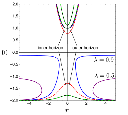
Figure 1: Contour map of ${Q}=0$ for $\lambda=0.9$ (blue), $\lambda=0.5$ (purple), $\lambda=\lambda_{\text{min}}$ (green), horizon (red dashed curve), and $g_{\varphi\varphi}=0$ (black dotted) with $\theta=\pi/6$ shown in the $(\bar{r},\Xi)$-plane, where $\Xi:=1-a^{2}/L^{2}$. Note that for a given value of $\theta$, there can be multiple caustics. For example the $\lambda=\lambda_{\text{min}}$ case here gives two caustic curves for the cisunital case, both of which coincide with a closed null curve. Both are located inside the event horizon. We also see that the caustics are outside the event horizon for transunital black holes ($\Xi<0$) but not for cisunital black holes ($\Xi>0$). Note that there are some ranges of $\Xi$ in which there is no black hole. This is due to the censorship condition given in Eq. (8). The lower panel is the zoom-in contours for the cisunital case.

Before we move on to other examples, let us comment on the CTCs in the transunital black hole spacetime. As discussed in 1906.01169 , the angular coordinate $\psi$ becomes timelike for $\theta<\theta_{a}:=\text{arccos}(L/a)$ (These regions can be excised so that the black hole topology is that of a sphere with two punctures). Thus, there are CTCs for the region close to the poles. These are not the CTCs we discussed here, which is in the $\varphi$-direction. It can be checked that the metric coefficient

$$g_{\varphi\varphi}=\frac{\sin^{2}\theta}{\rho^{2}\Xi^{2}}\left[-\Delta_{r}a^{2}\sin^{2}\theta+\Delta_{\theta}(r^{2}+a^{2})^{2}\right]$$ (33)

can become negative. This always happens at sufficiently large $r$. To see this, one can examine the leading term in $\Delta_{r}a^{2}\sin^{2}\theta$ and $\Delta_{\theta}(r^{2}+a^{2})^{2}$, that is, the coefficients of the $r^{4}$ terms. From this we can conclude that $g_{\phi\phi}<0$ for $a>L$ at large enough $r$.

In our discussion above, the closed null curve $g_{\varphi\varphi}=0$ is the one that corresponds to the caustics. It is not clear whether such closed causal curves are pathological from holographic point of view, since the (conformal) boundary metric (see 1906.01169 ) is free of CTC in the $\varphi$-direction. This is in contrast to the conical defect AdS₃ spacetime examined in 1508.04440 , whose CTCs extend to the boundary. Yet even in that case the holographic dual seemingly admits a consistent and controllable evolution even without imposing additional consistency constraints. In any case the physical relevance (or the lack thereof) is interesting but it is beyond the scope of work to discuss these issues in depth: our objective is merely to discuss the relationship between closed causal curve and NHC.

The aforementioned relationship between caustics and closed null curve also exist when they are inside a black hole horizon. This can be checked, e.g., in the case of asymptotically flat Kerr black hole, in the region $r<0$ “below” the ring singularity. For cisunital and transunital Kerr-AdS₅ black holes, see Fig. (1). It is worth noting at this point that the property that NHC can occur outside a black hole horizon is not unique to super-entropic black holes, since transunital black holes are not super-entropic in the usual sense, that is, with respect to thermodynamic volume (see Sec.(III) for definition). They can, however, be super-entropic with respect to mass 2006.09385 .

The method of searching for caustics explained thus far can be applied to various axisymmetric spacetimes. Therefore in the following parts of this work, we shall employ this method to discuss the caustics in a few other interesting spacetimes, with the hope to learn some shared properties and differences between them.

II.2 Taub-NUT

The Taub-NUT spacetime is a peculiar geometry that admits closed causal curves, but it also shares some similarities with Kerr black holes (in fact, it can be written in a Boyer-Lindquist-like coordinates in which the solution looks like a “twisting” black hole with the two hemispheres rotating in opposite directions 1610.05757 ; 1609.09721 ), so it provides another arena that we can explore to check the relationship between null hypersurface caustics and closed causal curves.

The metric tensor of the Taub-NUT spacetime can be written in the coordinates $(\tau,r,\theta,\varphi)$ as Bonner

$$g[\text{T-N}] =-U(r)\left[\operatorname{d}\!{\tau}+4a\sin^{2}{(\theta/2)}\operatorname{d}\!{\varphi}\right]^{2}+\dfrac{\operatorname{d}\!{r}^{2}}{U(r)}$$ (34)

$$+(r^{2}+a^{2})(\operatorname{d}\!{\theta}^{2}+\sin^{2}\theta\operatorname{d}\!{\varphi}^{2}),$$

where

$$U(r)=\dfrac{r^{2}-2Mr-a^{2}}{r^{2}+a^{2}}.$$ (35)

Here $a$ is not a rotation parameter but the NUT charge, which has no Newtonian analog.

Alternatively, in $(t,r,\theta,\varphi)$ coordinates, in which $t=\tau+2a\varphi$, we can write the metric as

$$g[\text{T-N}]= -U\operatorname{d}\!{t}^{2}-4aU\cos{\theta}\operatorname{d}\!{t}\operatorname{d}\!{\varphi}+\dfrac{\operatorname{d}\!{r}^{2}}{U}+(r^{2}+a^{2})\operatorname{d}\!{\theta}^{2}$$ (36)

$$+\left[-4a^{2}U\cos^{2}{\theta}+(r^{2}+a^{2})\sin^{2}{\theta}\right]\operatorname{d}\!{\varphi}^{2}.$$

To evaluate the null hypersurface, we need the inverse metric component $g^{tt}$:

$$g^{tt} =-\dfrac{g_{\varphi\varphi}}{g_{t\varphi}^{2}-g_{tt}g_{\varphi\varphi}}=\dfrac{4a^{2}U\cos^{2}{\theta}-(r^{2}+a^{2})\sin^{2}{\theta}}{(r^{2}+a^{2})U\sin^{2}{\theta}}$$ (37)

$$=\dfrac{4a^{2}}{(r^{2}+a^{2})}\cot^{2}{\theta}-\dfrac{1}{U(r)}.$$

For $v=t+r_{*}$, the null hypersurface is given by

$$g^{\mu\nu}\partial_{\mu}v\partial_{\nu}v=g^{tt}+g^{rr}(\partial_{r}r_{*})^{2}+g^{\theta\theta}(\partial_{\theta}r_{*})^{2}=0,$$ (38)

which yields

$$(\partial_{r}r_{*})^{2} =\dfrac{r^{2}+a^{2}-a^{2}\lambda U}{U^{2}(r^{2}+a^{2})}$$ (39)

$$=\dfrac{(r^{2}+a^{2})^{2}-a^{2}\lambda(r^{2}-2Mr-a^{2})}{U^{2}(r^{2}+a^{2})^{2}},$$

and

$$(\partial_{\theta}r_{*})^{2}=a^{2}(\lambda-4\cot^{2}{\theta}).$$ (41)

From the second equation, we get the bound on the separation constant

$$\lambda\geqslant 4\cot^{2}{\theta}:=\lambda_{\text{min}}.$$ (42)

Figure 2: Contour map of the caustics $[r^{2}+a^{2}-\lambda U(r)]=0$ for different separation constants $\lambda$ (blue, purple, green), horizon radii (dashed red), and the boundary of the closed timelike curve region, $g_{\varphi\varphi}=0$ (dotted black), for the choice $\theta=\pi/6$, in the Taub-NUT spacetime.

In Fig. (2), the caustics condition $(r^{2}+a^{2})^{2}-a^{2}\lambda(r^{2}-2Mr-a^{2})=0$, the horizon condition $r^{2}-2Mr-a^{2}=0$, as well the CTC condition (null closed curve $g_{\varphi\varphi}=0$) for given $\theta$ on $(r,a)$-plane are plotted. In these plots, for definiteness we have set $\theta=\pi/6$, hence, $\lambda_{\text{min}}=12$.

Once again, we observe that the null closed curve coincides with the NHC with minimal separation constant. This is true both outside and inside the horizon. Note that the negative $r$ region is connected with the positive $r$ region by the 2-surface of finite area at $r=0$ (at which the curvature is finite and hence not a singularity) 1610.06135 .

II.3 Tipler cylinder

As another example of spacetime with CTC, we consider one of the archetypal example of time machine: the Tipler cylinder Tipler , which is an infinitely long and massive spinning object. The metric for the whole region of the spacetime is written in the following form:

$$g[\text{TIP}]=-F\operatorname{d}\!{t}^{2}+2M\operatorname{d}\!{t}\operatorname{d}\!{\varphi}+H(\operatorname{d}\!{r}^{2}+\operatorname{d}\!{z}^{2})+L\operatorname{d}\!{\varphi}^{2}.$$ (43)

The $z$-axis corresponds to the spin axis of the cylinder. The inner region of the surface whose radius is $R$ is given by

$$F=1,\ M=ar^{2},\ H=e^{-a^{2}r^{2}},\ L=r^{2}(1-a^{2}r^{2}),$$ (44)

where $a$ is the angular velocity of the cylinder. Separating the PDE $g^{\mu\nu}\partial_{\mu}v\partial_{\nu}v=0$ with the separation constant $\lambda$, we obtain

$$(\partial_{r}r_{*})^{2}=\dfrac{1-a^{2}r^{2}-\lambda e^{a^{2}r^{2}}}{e^{a^{2}r^{2}}},$$ (45)

$$(\partial_{z}r_{*})^{2}=\lambda.$$ (46)

Considering these equations and $L$, we will see that caustics with $\lambda=\lambda_{\text{min}}=0$ gives the boundary of the CTC region $g_{\varphi\varphi}=0$.

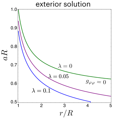
Figure 3: NHC curves and $g_{\varphi\varphi}=0$ (black dotted) for interior solution (upper panel) and exterior solution (lower panel) for several values of $\lambda$ in the Tipler cylinder spacetime.

The exterior solution is classified into the following three classes depending on the radius $R$: $0<aR<1/2$, $aR=1/2$, and $1/2<aR<1$. The upper bound $aR<1$ stems from the fact that the surface velocity of the cylinder is supposed to be slower than the speed of light. According to Tipler , only the third case possesses CTC, therefore, we focus on this case here. The metric functions are

$$F=\dfrac{r\sin{(\beta-\gamma)}}{R\sin{\beta}},\ M=\dfrac{r\sin{(\beta+\gamma)}}{\sin{2\beta}},$$ (47)

$$H=e^{-a^{2}R^{2}}\left(\dfrac{r}{R}\right)^{-2a^{2}R^{2}},\ L=\dfrac{Rr\sin{(3\beta+\gamma)}}{2\sin{2\beta}\cos{\beta}},$$ (48)

with

$$\beta=\tan^{-1}{\left(4a^{2}R^{2}-1\right)^{1/2}},\ \gamma=\left(4a^{2}R^{2}-1\right)^{1/2}\log{(r/R)}.$$ (49)

The PDE for the NHC yields

$$(\partial_{r}r_{*})^{2}=\dfrac{R\sin{(3\beta+\gamma)}-2\lambda e^{a^{2}R^{2}}(r/R)^{2a^{2}R^{2}}r\sin{2\beta}\cos{\beta}}{2r\sin{2\beta}\cos{\beta}e^{a^{2}R^{2}}(r/R)^{2a^{2}R^{2}}},$$ (50)

$$(\partial_{z}r_{*})^{2}=\lambda.$$ (51)

The NHC curves and the closed null curve $g_{\varphi\varphi}=0$ for both interior and exterior solutions are shown in Fig. 3.

To conclude, all spacetimes discussed in this subsection have CTCs. Regardless of the positions of the CTCs, i.e., whether they are located inside or outside the horizon, the NHCs with minimum separation constant coincide with the $g_{\varphi\varphi}=0$ closed null curve.

III Null Hypersurface Caustics and Super-Entropic Black Holes

Since the super-entropic black hole studied in 2007.04354 is free of closed causal curve, there might be some connection between the presence of NHC outside a black hole horizon and the property that said black hole is super-entropic. This is what we propose to study in this section. Let us start with a brief explanation on what it means to be “super-entropic”. In the recent years, the inclusion of the negative cosmological constant as a thermodynamical variable (a “pressure”) in anti-de Sitter spacetime, and its subsequent rich phenomenology, dubbed “black hole chemistry”, has received a lot of attention (see kn:chemistry for a review). Specifically, the thermodynamical pressure is $P=-\Lambda/8\pi G$, where we have restored the Newton’s gravitational constant for clarity. The “thermodynamical volume” $V$ is defined as the thermodynamic conjugate $\partial M/\partial P$. This notion of volume has no geometric meaning in general, for example, it can even be negative for Taub-NUT 1405.5941 . Nevertheless, for static charged or neutral black holes, it coincides with the naive spherical volume $V=({4}/{3})\pi r_{+}^{3}$. There is a conjecture called the “reverse isoperimetric inequality” kn:cvetgib , which states that the AdS-Schwarzschild black hole has the largest entropy among all black holes with the same thermodynamic volume. In this sense AdS-Schwarzschild is the most stable configuration (under the second law of thermodynamics, the black hole would prefer to evolve towards the state with largest entropy). A “super-entropic” black holes are black holes that violate this inequality. There are only a few known super-entropic black holes, so it is possible that the reverse isoperimetric inequality holds for “most” black holes (though the exact meaning of “most” has yet to be defined; in 1411.4309 it is conjectured that all black holes with compact horizon would satisfy the reverse isoperimetric inequality).

The super-entropic Kerr-AdS black hole 1411.4309 ; 1504.07529 ; 1401.3107 is constructed by first re-scaling the coordinate $\phi$ into $\tilde{\phi}:=\phi/\Xi$ and then taking the limit $a\to L$ (this is referred to as the “ultra-spinning” limit). The new coordinate $\tilde{\phi}$ is then (re-)compactified. Recently there has been some doubt on its true status as a counter-example to the reverse isoperimetric inequality 1911.12817 . Nevertheless, motivated by 2007.04354 , let us examine two other known examples of super-entropic black holes.

III.1 Ultra-Spinning Kerr-Sen-AdS Black Hole

Kerr-Sen black hole sen is a rotating charged black hole which is an exact solution of the low-energy heterotic string theory (EMDA theory, short for “Einstein-Maxwell-Dilaton-Axion” theory), obtained via applying a solution generating technique to the Kerr solution. The Lagrangian of the theory is given as

$${\cal{L}}=\sqrt{-g}\left[R-\dfrac{1}{2}(\partial\phi)^{2}-e^{-\phi}F^{2}-\dfrac{1}{12}e^{-2\phi}H^{2}\right],$$ (52)

where $F^{2}=F_{\mu\nu}F^{\mu\nu}$ is the square of the Maxwell field tensor, $\phi$ is the dilaton field, and $H:=-e^{2\phi}\star\operatorname{d}\!{\chi}$ is a third-rank tensor field. Here $\chi$ denotes the axion pseudoscalar Hodge-dual to $H$. The solution with the cosmological constant can also be obtained.

Recently, Wu et al. found that an ultra-spinning Kerr-Sen-AdS₄ black hole can be super-entropic but not always so, depending on the values of the parameters Wu2020 . We shall now check whether super-entropy is related to NHC in this spacetime geometry.

The metric of the ultraspininng Kerr-Sen AdS₄ black hole is

$$g[\text{K-S}]= -\dfrac{\Delta_{r}}{\Sigma}\left(\operatorname{d}\!{t}-L\sin^{2}{\theta}\operatorname{d}\!{\varphi}\right)^{2}+\dfrac{\Sigma}{\Delta_{r}}\operatorname{d}\!{r}^{2}+\dfrac{\Sigma}{\sin^{2}{\theta}}\operatorname{d}\!{\theta}^{2}$$ (53)

$$+\dfrac{\sin^{4}{\theta}}{\Sigma}\left[L\operatorname{d}\!{t}-(r^{2}+2br+L^{2})\operatorname{d}\!{\varphi}\right]^{2},$$

where $b:=q^{2}/(2m)$ is the dilatonic scalar charge, while $m$ and $q$ are the mass and electric charge parameter of the black hole, and

$$\Delta_{r}=(r^{2}+2br+L^{2})^{2}L^{-2}-2mr,\ \ \Sigma=r^{2}+2br+L^{2}\cos^{2}{\theta}.$$ (54)

As discussed in Wu2020 , the black hole is super-entropic for $b/L<1$ and not super-entropic (“sub-entropic”) for $b/L>1$. Note that in order to discuss super/sub-entropy, we need to restrict the parameters $m$ and $b$ so that the black hole spacetime still admits a horizon. It can nevertheless be shown that caustics can appear even around naked singularities, but without a horizon we cannot discuss the notion of entropy.

The $tt$, $t\varphi$, and $\varphi\varphi$ components of the metric are:

$$g_{tt}=\dfrac{1}{\Sigma}\left(-\Delta_{r}+L^{2}\sin^{4}{\theta}\right),$$

$$g_{t\varphi}=\dfrac{L\sin^{2}{\theta}}{\Sigma}\left[\Delta_{r}-\sin^{2}{\theta}(r^{2}+2br+L^{2})\right],$$

$$g_{\varphi\varphi}=\dfrac{2mrL^{2}}{\Sigma}\sin^{4}{\theta}.$$

Since $g_{\varphi\varphi}$ is always positive, much like the ultraspinning Kerr-AdS black hole, the ultraspinning Kerr-Sen-AdS₄ black hole is free of closed causal curve in the entire spacetime. To calculate $g^{tt}$, we need to compute $D:=g_{t\varphi}^{2}-g_{tt}g_{\varphi\varphi}$. The expression is simple:

$$D=\Delta_{r}\sin^{4}{\theta}.$$ (55)

Using this, the inverse component $g^{tt}$ is readily obtained to be

$$g^{tt}=-\dfrac{g_{\varphi\varphi}}{D}=-\dfrac{2mrL^{2}}{\Delta_{r}\Sigma}.$$ (56)

Since the null hypersurface is given by

$$g^{\mu\nu}\partial_{\mu}(t+r_{*})\partial_{\nu}(t+r_{*})=0,$$ (57)

we obtain

$$-\dfrac{2mrL^{2}}{\Delta_{r}}+\Delta_{r}(\partial_{r}r_{*})^{2}+\sin^{2}{\theta}(\partial_{\theta}r_{*})^{2}=0.$$ (58)

As emphasized in 2003.14349 , even in the asymptotically flat case, the Kerr-Sen spacetime is of Petrov Type I 9504139 , thus, a priori, one does not expect it to have a Carter-like constant. Nevertheless, the Hamilton-Jacobi equation is separable for the geodesics 1712.06667 . For our asymptotically AdS case, Introducing a constant for the separation of variables as $L^{2}\lambda$, this equation yields

$$(\partial_{r}r_{*})^{2}=L^{2}\dfrac{(2mr-\lambda\Delta_{r})}{\Delta_{r}^{2}},\ \ (\partial_{\theta}r_{*})^{2}=\dfrac{L^{2}\lambda}{\sin^{2}{\theta}}.$$ (59)

Therefore the caustics condition is $2mr-\lambda\Delta_{r}=0$. We plot this condition and the horizon condition $\Delta_{r}=0$ in Fig. (4).

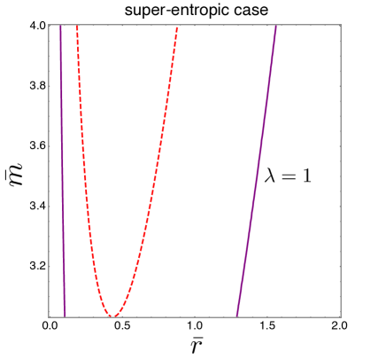
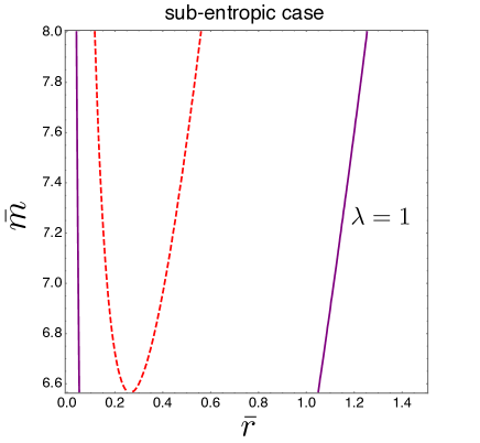
Figure 4: For the ultra-spinning Kerr-Sen-AdS₄ black holes: contours of the caustics $2mr-\lambda\Delta_{r}=0$ with $\lambda=1$ (purple), and horizon curve (dashed red curve) on the $(\bar{r},\bar{m})$-plane for super-entropic case ($\bar{b}=0.5$) and sub-entropic case ($\bar{b}=1.5$), where quantities with bar are normalized by $L$. There exist caustics outside the horizon in both super/sub-entropic cases.

We note that there exist caustics outside the horizon in both super and sub-entropic cases. The result seems to indicate that the existence of NHC outside the horizon is not related to whether the black holes is super-entropic or not at least for Kerr-Sen-AdS case. In the following sub-section, we will see that this is also the case for charged BTZ black strings.

III.2 Charged BTZ Black String

Another example of the super-entropic black hole is the charged BTZ spacetime Johnson2020 . To make a four-dimensional solution, we consider an extra fourth-dimension in the $z$-direction (charged BTZ black string). The metric is written as

$$g[\text{BTZ}]=-f(r)\operatorname{d}\!{t}^{2}+\frac{1}{f(r)}\operatorname{d}\!{r}^{2}+r^{2}\operatorname{d}\!{\varphi}^{2}+h(z)\operatorname{d}\!{z}^{2},$$ (60)

where

$$f(r)=-8M-\dfrac{{q}^{2}}{2}\log{(r/L)}+\dfrac{r^{2}}{L^{2}},$$ (61)

and $h(z)$ is an arbitrary positive definite function. The cosmological constant sets the length scale via $\Lambda:=-1/L^{2}$. As discussed in the Appendix B, this spacetime can be super-entropic, depending on the charge parameter $q$ and the functional form of the warp factor $h(z)$. However, the spacetime geometry is always free of closed causal curves since $g_{\varphi\varphi}\geqslant 0$.

To define the null hypersurfaces, we again start by introducing ingoing and outgoing Eddington-Finkelsteing coordinates:

$$\ \ u=t-r_{*},\ \ v=t+r_{*},$$ (62)

where $r_{*}=r_{*}(r,z)$ is the tortoise coordinate. The equation that null hypersurface satisfies is

$$g^{\mu\nu}\partial_{\mu}v\partial_{\nu}v=g^{tt}+g^{rr}(\partial_{r}r_{*})^{2}+g^{zz}(\partial_{z}r_{*})^{2}=0.$$ (63)

This PDE simplifies into

$$-\dfrac{1}{f(r)}+f(r)(\partial_{r}r_{*})^{2}+\dfrac{1}{h(z)}(\partial_{z}r_{*})^{2}=0.$$ (64)

Therefore, after introducing the constant for the separation of variables $\lambda$, we can obtain

$$(\partial_{r}r_{*})^{2}=\dfrac{1-f\lambda}{f^{2}},\ \ (\partial_{z}r_{*})^{2}=\lambda h(z).$$ (65)

The computation is similar to the other cases explored thus far. The end result yields

$$1-f\lambda=0,$$ (66)

which gives the caustics curve. Note that $\lambda\geqslant 0$ since $h(z)>0$. We plot this condition and the horizon condition $f=0$ on the $(r,q)$-plane in Fig. 5.

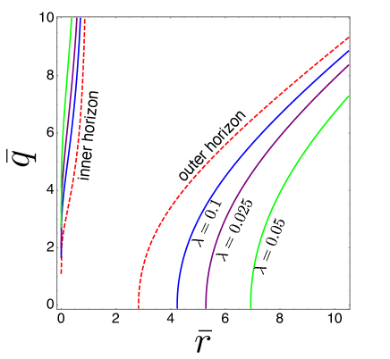
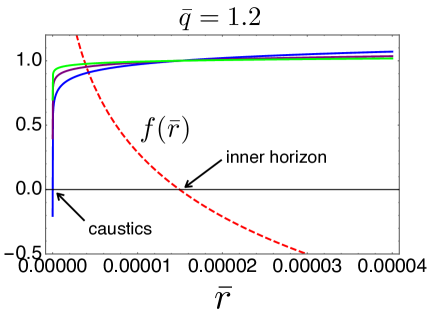
Figure 5: Contour map of the charged BTZ black string caustics $1-f\lambda=0$ for several values of $\lambda=0.025$ (green), $0.05$ (purple), $0.1$ (blue), and the horizon curve (dashed red curve) on the $(\bar{r},\bar{q})$-plane, where $\bar{r}:=r/L$ and $\bar{q}:=q/L$. The lower panel shows the positions of the inner horizon and caustics for fixed $\bar{q}$ to clarify their behaviors around the inner horizon (red dashed curve) for small $\bar{q}$ in the upper panel.

For arbitrary $\lambda$ and arbitrary value of the charge, the caustic curve is outside the horizon. Specifically, and surprisingly, this is also the case for neutral BTZ black string. The charged BTZ black string example shows that it is possible that a class of solution can be super-entropic only for some choices of the parameter and metric coefficients, yet there are always NHC present outside the event horizon.

IV Discussion

In this work, we have discussed the null hypersurface caustics (NHC) of the following spacetimes: transunital AdS₅-Kerr, Taub-NUT, Tipler cylinder, charged (non-rotating) BTZ string, and ultra-spinning Kerr-Sen-AdS₄. Among these, transunital black holes, Tipler cylinder, and Taub-NUT spacetimes admit closed timelike curves (CTC), and the NHC with minimal separation constant coincides with the closed null curve, which corresponds to the boundary of the CTC-region. This can occur outside the black hole horizon. A general proof of this relationship is difficult. The main idea involved in the calculations is to express $g^{tt}$ as $-g_{\varphi\varphi}/D$, however the separation of variables requires knowledge on the detailed form of $g_{\varphi\varphi}$. Such proof should be possible for more restricted class of metric, but then it is doubtful whether such result would shed more light to our understanding.

The relationship between CTC and NHC shows that indeed the caustics in null hypersurfaces reflect the underlying causal structures of the spacetime geometry. In this work we are agnostic about whether CTCs are definitely bad, as it is a matter of ongoing debate, which is outside the scope of our work. (See, e.g., 1912.04702 ; 1711.08334 , which essentially argued that although point particle can travel on a CTC, any macroscopic objects would be constrained by the second law of thermodynamics. See also 2005.05748 .)

The ultra-spinning Kerr-Sen-AdS₄ black holes can be either super-entropic or not, depending on the values of the black hole parameters. Regardless of the fact that such black holes are super-entropic, NHCs appear outside their horizon. Together with the ultra-spinning Kerr-AdS₄ spacetime, our results suggest that black holes that can become super-entropic might have NHC outside the horizon. Further evidence is provided by the charged BTZ black string, which is also super-entropic for some choices of the charge parameter and the warp factor. However, for the charged BTZ black string, all of them – even the sub-entropic ones – have NHC outside the event horizon. More examples of super-entropic black holes are required to study the relationship between super-entropy and NHC.

Appendix A Derivation of the Metric in Eq. (25)

Using Eq. (18) and Eq. (23), we obtain

$$\operatorname{d}\!{r}=\dfrac{Q\Delta_{r}}{Q^{2}\Delta_{\theta}+P^{2}\Delta_{r}}\left(\Delta_{\theta}\operatorname{d}\!{r}_{*}-\nu P^{2}\operatorname{d}\!{\lambda}\right),$$ (67)

$$\operatorname{d}\!{\theta}=\dfrac{P\Delta_{\theta}}{Q^{2}\Delta_{\theta}+P^{2}\Delta_{r}}\left(\Delta_{r}\operatorname{d}\!{r}_{*}+\nu Q^{2}\operatorname{d}\!{\lambda}\right).$$ (68)

Substituting these into $g_{rr}$ and $g_{\theta\theta}$ terms, we get

$$\dfrac{\rho^{2}}{\Delta_{r}}\operatorname{d}\!{r}^{2}+\dfrac{\rho^{2}}{\Delta_{\theta}}\operatorname{d}\!{\theta}^{2}$$

$$=\dfrac{1}{\Xi^{2}R^{2}}\left(\Delta_{r}\Delta_{\theta}\operatorname{d}\!{r}_{*}^{2}+\nu^{2}P^{2}Q^{2}\operatorname{d}\!{\lambda}^{2}\right),$$ (69)

whereas the terms with $g_{tt},\ g_{t\varphi}$, $g_{\varphi\varphi}$ can be rewritten as

$$g_{tt}\operatorname{d}\!{t}^{2}+2g_{t\varphi}\operatorname{d}\!{t}\operatorname{d}\!{\varphi}+g_{\varphi\varphi}\operatorname{d}\!{\varphi}^{2}$$

$$=\left(g_{tt}-\dfrac{g_{t\varphi}^{2}}{g_{\varphi\varphi}}\right)\operatorname{d}\!{t}^{2}+\dfrac{g_{t\varphi}^{2}}{g_{\varphi\varphi}}\operatorname{d}\!{t}^{2}+2g_{t\varphi}\operatorname{d}\!{t}\operatorname{d}\!{\varphi}+g_{\varphi\varphi}\operatorname{d}\!{\varphi}^{2}$$

$$=-\dfrac{D}{g_{\varphi\varphi}}\operatorname{d}\!{t}^{2}+g_{\varphi\varphi}(\operatorname{d}\!{\varphi}-\omega\operatorname{d}\!{t})^{2}=-\dfrac{\Delta_{r}\Delta_{\theta}}{\Xi^{2}R^{2}}\operatorname{d}\!{t}^{2}+g_{\varphi\varphi}\operatorname{d}\!{\varpi}^{2}.$$ (70)

Thus we obtain Eq. (25).

Appendix B Is the charged BTZ black string super-entropic?

Although three-dimensional charged BTZ spacetime is a super-entropic black hole Johnson2020 , it does not trivially follow that the solution with an “extra direction” ($z$-direction) is always super-entropic.

Following the procedure which has already been discussed in the literature kn:cvetgib ; 1411.4309 , we evaluate whether the reverse isoperimetric inequality

$${\cal{R}}:=\left[\frac{(D-1)V}{\omega_{D-2}}\right]^{\frac{1}{D-1}}\left[\frac{\omega_{D-2}}{\cal{A}}\right]^{\frac{1}{D-2}}\geqslant 1,$$ (71)

holds. Here $D$ is the spacetime dimension and $\omega_{D}$ stands for the area of the space orthogonal to constant $(t,r)$. The horizon area ${\cal{A}}$ can be obtained from the metric as follows

$${\cal{A}}=2\pi r_{+}\int_{-\infty}^{+\infty}h(z)dz:=2\pi r_{+}H,$$ (72)

where $r_{+}$ is the radius of the outer horizon.

One immediately notices that one must constrain the horizon area to be finite in order to have any chance for the black string to be super-entropic. This means that the warp factor $h(z)$ should be chosen in such a way that the area integral converges.

Now, $M$ is the energy (mass) of the black hole obtained from the horizon condition $f(r_{+})=0$:

$$M=\dfrac{r_{+}^{2}}{8L^{2}},$$ (73)

and $P$ is the pressure given with the cosmological constant $\Lambda$ as

$$P=-\dfrac{\Lambda}{8\pi}=\dfrac{(D-2)(D-1)}{16\pi L^{2}}.$$ (74)

The thermodynamic volume $V$ is computed using the formula in black hole chemistry kn:chemistry :

$$V=\left(\dfrac{\partial M}{\partial P}\right)_{S,q},$$ (75)

the subscript means that the entropy and charge of the black hole should be fixed when taking the partial derivative. Using (73) and (74), the thermodynamic volume is

$$V=-\dfrac{\pi q^{2}L^{2}}{12}+\dfrac{\pi}{3}r_{+}^{2}.$$ (76)

Therefore, for the present metric ${\cal{R}}$ is obtained as

$${\cal{R}}=\left[\dfrac{3V}{\omega_{2}}\right]^{1/3}\left[\dfrac{\omega_{2}}{{\cal{A}}}\right]^{1/2}=H^{-1/3}r_{+}^{-1/2}\left[\dfrac{r_{+}^{2}}{2}-\dfrac{q^{2}L^{2}}{8}\right]^{1/3},$$ (77)

where we have $\omega_{2}=2\pi H$. Depending on the parameter $q$ and the integrated warp factor $H$, the ratio ${\cal{R}}$ can be either larger or smaller than unity. That is, charged BTZ black string can be super-entropic but only for suitable choices of the charge value and the form of the warped function.

References

- (1) Richard Arnowitt, Stanley Deser, Charles W. Misner, “Dynamical Structure and Definition of Energy in General Relativity”, Phys. Rev. 116 (1959) 1322.
- (2) Richard Arnowitt, Stanley Deser, Charles W. Misner, Gravitation: An Introduction to Current Research, ed. L. Witten (New York: Wiley) Chap. 7, 1962.
- (3) Albert Huber, “Null Foliations of Spacetime and the Geometry of Black Hole Horizons”, [arXiv:1908.08739 [gr-qc]].
- (4) Patrick R. Brady, Serge Droz, Werner Israel, Sharon M. Morsink, “Covariant Double-Null Dynamics: (2+2)-Splitting of the Einstein Equations”, Class. Quant. Grav. 13 (1996) 2211, [arXiv:gr-qc/9510040].
- (5) Giulio Caciotta, Francesco Nicolò, “Local and Global Analytic Solutions for a Class of Characteristic Problems of the Einstein Vacuum Equations in the ’Double Null Foliation Gauge”’, Annales Henri Poincaré 13 (2012) 1167, [arXiv:1103.3538 [gr-qc]].
- (6) Frans Pretorius, Werner Israel, “Quasi-Spherical Light Cones of the Kerr Geometry”, Class. Quant. Grav. 15 (1998) 2289, [arXiv:gr-qc/9803080].
- (7) Abdulrahim Al Balushi, Robert B. Mann, “Null Hypersurfaces In Kerr-(A)dS Spacetimes”, Class. Quant. Grav. 36 (2019) 245017, [arXiv:1909.06419 [gr-qc]].
- (8) Michael T.N. Imseis, Abdulrahim Al Balushi, Robert B. Mann, “Null Hypersurfaces in Kerr-Newman-AdS Black Hole and Super-Entropic Black Hole Spacetimes”, [arXiv:2007.04354 [gr-qc]].
- (9) Brett McInnes, “Cosmic Censorship for AdS5-Kerr”, Nucl. Phys. B 950 (2020) 114845, [arXiv:1906.01169 [hep-th]].
- (10) Brett McInnes, “Cosmic Censorship and Holography”, [arXiv:1911.08222 [hep-th]].
- (11) Brett McInnes, “Fragmentation of AdS5-Kerr Black Holes”, [arXiv:2005.03869 [gr-qc]].
- (12) Brett McInnes, Yen Chin Ong, “Event Horizon Wrinklification”, [arXiv:2006.09385 [gr-qc]].
- (13) Gary W. Gibbons, Malcolm J. Perry, Christopher N. Pope, “The First Law of Thermodynamics for Kerr-anti-de Sitter Black Holes”, Class. Quant. Grav. 22 (2005) 1503, [arXiv:hep-th/0408217].
- (14) Wenbo Chen, Hong Lü, Christopher Pope, “Kerr-de Sitter Black Holes with NUT Charges”, Nucl. Phys. B 762 (2007) 38, [arXiv:hep-th/0601002].
- (15) Wenbo Chen, Hong Lü, Christopher Pope, “General Kerr-NUT-AdS Metrics in All Dimensions”, Class. Quant. Grav. 23 (2006) 5323, [arXiv:hep-th/0604125].
- (16) Irina Arefeva, Andrey Bagrov, Petter Saterskog, Koenraad Schalm, “Holographic Dual of a Time Machine”, Phys. Rev. D 94 (2016) 044059, [arXiv:1508.04440 [hep-th]].
- (17) Yen Chin Ong, “Twisted Black Hole Is Taub-NUT”, JCAP 01 (2017) 001, [arXiv:1610.05757 [gr-qc]].
- (18) Hongsheng Zhang, “Twisted Spacetime in Einstein Gravity”, [arXiv:1609.09721 [gr-qc]].
- (19) William B. Bonnor, “A New Interpretation of the NUT Metric in General Relativity”, Proc. Camb. Phil. Soc. 66 (1969) 145.
- (20) Finnian Gray, Jessica Santiago, Sebastian Schuster, Matt Visser, ““Twisted” Black Holes Are Unphysical”, Mod. Phys. Lett. A 32 (2017) 1771001, [arXiv:1610.06135 [gr-qc]].
- (21) Frank J. Tipler, “Rotating Cylinders and the Possibility of Global Causality Violation”, Phys. Rev. D 9 (1974) 2203.
- (22) David Kubiznak, Robert B. Mann, Mae Teo, “Black Hole Chemistry: Thermodynamics With Lambda”, Class. Quantum Grav. 34 (2017) 063001, [arXiv:1608.06147 [hep-th]].
- (23) Clifford V. Johnson, “Thermodynamic Volumes for AdS-Taub-NUT and AdS-Taub-Bolt”, Class. Quant. Grav. 31 (2014) 235003, [arXiv:1405.5941 [hep-th]].
- (24) Mirjam Cvetic, Gary W. Gibbons, David Kubiznak, Christopher N. Pope”, “Black Hole Enthalpy and an Entropy Inequality for the Thermodynamic Volume”, Phys. Rev. D 84 (2011) 024037, [arXiv:1012.2888 [hep-th]].
- (25) Robie A. Hennigar, David Kubiznak, Robert B. Mann, “Super-Entropic Black Holes”, Phys. Rev. Lett. 115 (2015) 031101, [arXiv:1411.4309 [hep-th]].
- (26) Robie A. Hennigar, David Kubiznak, Robert B. Mann, Nathan Musoke, “Ultraspinning Limits and Super-Entropic Black Holes”, JHEP 1506 (2015) 096, [arXiv:1504.07529 [hep-th]].
- (27) Dietmar Klemm, “Four-Dimensional Black Holes With Unusual Horizons”, Phys. Rev. D 89 (2014) 084007, [arXiv:1401.3107 [hep-th]].
- (28) Michael Appels, Leopoldo Cuspinera, Ruth Gregory, Pavel Krtous, David Kubiznak, “Are Superentropic Black Holes Superentropic?”, JHEP 02 (2020) 195, [arXiv:1911.12817 [hep-th]].
- (29) Ashoke Sen, “Rotating Charged Black Hole Solution in Heterotic String Theory”, Phys. Rev. Lett. 69 (1992) 1006, [arXiv:hep-th/9204046].
- (30) Di Wu, Puxun Wu, Hongwei Yu, Shuang-Qing Wu, “Are Ultra-Spinning Kerr-Sen-AdS4 Black Holes Always Super-Entropic ?”, Phys. Rev. D 102 (2020) 044007, [arXiv:2007.02224 [gr-qc]].
- (31) Sérgio Vinicius M. C. B. Xavier, Pedro V. P. Cunha, Luís C. B. Crispino, Carlos A. R. Herdeiro, “Shadows of Charged Rotating Black Holes: Kerr-Newman Versus Kerr-Sen”, Int. J Modern Phys. D (2020) 2041005, [arXiv:2003.14349 [gr-qc]].
- (32) Alexander Burinskii, “Some Properties of the Kerr Solution to Low-Energy String Theory”, Phys. Rev. D 52 (1995) 5826, [arXiv:hep-th/9504139].
- (33) Roman A. Konoplya, Alexander Zhidenko, “Quasinormal Modes of Massive Fermions in Kerr Spacetime: Long-Lived Modes and the Fine Structure”, Phys. Rev. D 97 (2018) 084034, [arXiv:1712.06667 [gr-qc]].
- (34) Clifford V. Johnson, “Instability of Super-Entropic Black Holes in Extended Thermodynamics”, Mod. Phys. Lett. A 33 (2020) 2050098, [arXiv:1906.00993 [hep-th]].
- (35) Carlo Rovelli, “Can We Travel to the Past? Irreversible Physics Along Closed Timelike Curves”, [arXiv:1912.04702 [gr-qc]].
- (36) Małgorzata Bartkiewicz, Andrzej Grudka, Ryszard Horodecki, Justyna Łodyga, Jacek Wychowaniec, “Closed Timelike Curves and the Second Law of Thermodynamics”, Phys. Rev. A 99 (2019) 022304, [arXiv:1711.08334 [gr-qc]].
- (37) Claudio F. Paganini, “Nothing Happens on Closed Causal Curves”, [arXiv:2005.05748 [gr-qc]].