Polarization as a signature of local parity violation in hot QCD matter

Abstract

We show that local parity violation due to chirality imbalance in relativistic nuclear collisions can be revealed by measuring the projection of the polarization vector onto the momentum, i.e. the helicity, of final state baryons. The proposed method does not require a coupling to the electromagnetic field, like in the Chiral Magnetic Effect. By using linear response theory, we show that, in the presence of a chiral imbalance, the spin 1/2 baryons and anti-baryons receive an additional contribution to the polarization along their momentum and proportional to the axial chemical potential. The additional, parity-breaking, contribution to helicity can be detected by studying helicity-helicity azimuthal angular correlation.

I Introduction

The vacuum state of the Quantum Chromodynamics (QCD) plays a crucial role in the understanding of strong interactions phenomenology. The study the Quark Gluon Plasma (QGP) in relativistic heavy ion collisions provides essential information on QCD at high temperature, but it may also shed light on QCD vacuum. Indeed, thanks to the high temperatures, non-trivial topological configurations can be produced with sufficiently high probability McLerran et al. (1991) through a classical thermal transition process called sphaleron Manton (1983). Given the random nature of this process, the topological charge fluctuates on an event by event basis Kharzeev et al. (2002) in nuclear collisions and vanishes when averaged over many events.

The local topological fluctuations are transferred to the chirality of fermions through the axial anomaly Adler (1969); Bell and Jackiw (1969) and an imbalance between right-handed and left-handed quarks, hence a local parity violation, is thereby generated Kharzeev et al. (1998). Thanks to the chiral symmetry of QGP, the imbalance is maintained through all the evolution of the plasma Kharzeev et al. (2008). The asymmetry between the number of right-handed and left-handed fermions can be included in a hydrodynamic picture with an axial chemical potential Kharzeev et al. (2008); Fukushima et al. (2008).

Local parity violation has been investigated in heavy-ion collisions via the so-called Chiral Magnetic Effect (CME) Fukushima et al. (2008). This phenomenon, experimentally found in condensed matter, is the generation of an electric current parallel to a magnetic field and proportional to the axial chemical potential. The CME is expected to bring about a charge-dependent azimuthal asymmetry in the spectrum of produced particles Abelev et al. (2009). However, backgrounds unrelated to the CME are difficult to evaluate Kharzeev et al. (2016); Bzdak et al. (2013) and dedicated experiments with isobar collisions Voloshin (2010); Deng et al. (2016); Adam et al. (2019a) have been proposed and are currently ongoing to finally demonstrate its existence. From the phenomenological standpoint, there are large uncertainties on the magnitude of the magnetic field in the plasma phase and this affects the quantitative assessment of the CME.

Lately, the STAR experiment at RHIC measured a global $\Lambda$ polarization Adamczyk et al. (2017) which turned out to be in very good agreement with predictions based on the hydrodynamic model of the QGP Becattini and Lisa . Also, the experiments proved to be able to measure it differentially in momentum space Adam et al. (2018, 2019b). These findings have opened a new window in the field of relativistic heavy ion physics with spin and polarization being newly available probes to study the QGP and its properties.

In this work, we propose to study and detect local parity violation by measuring the longitudinal component of polarization, that is helicity, of baryons produced in the collision, particularly $\Lambda$ hyperons. We will show that, if the axial chemical potential does not vanish at hadronization, the helicity of baryons is predicted to have an additional, parity-breaking, contribution with a specific azimuthal dependence in the transverse momentum plane. A similar idea was put forward by the authors of ref. Finch and Murray (2017), who proposed to correlate net helicity of $\Lambda$’s with charge separation due to CME. In fact, our proposed method does not require, like in the CME, the mediation of the electromagnetic field and it thus allows to evade some of the related uncertainties.

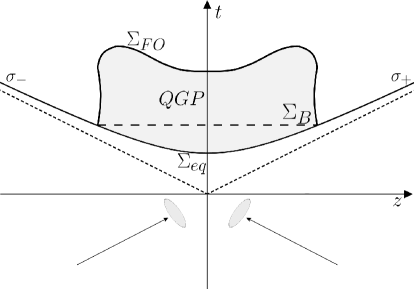
Figure 1: Space-time diagram of a relativistic nuclear collision in the center-of-mass frame. $\Sigma_{\textup{eq}}$ is the 3D hypersurface where local thermodynamic equilibrium is achieved, $\Sigma_{\textup{FO}}$ is the freeze-out hypersurface. The $\sigma_{\pm}$ are the side branches subsets of $\Sigma_{\textup{eq}}$ and $\Sigma_{\textup{B}}$ is the portion of hyperplane connecting the limiting surfaces of $\Sigma_{\textup{FO}}$.

II Polarization induced by an axial chemical potential

The mean spin vector of a spin $1/2$ hadron in a nuclear collision can be calculated by using the formula Becattini (2021)

$$S^{\mu}(p)=\frac{1}{2}\frac{\int_{\Sigma}{\rm d}\Sigma\cdot p\,{\rm tr}\left[\gamma^{\mu}\gamma^{5}W_{+}(x,p)\right]}{\int_{\Sigma}{\rm d}\Sigma\cdot p\,{\rm tr}\left[W_{+}(x,p)\right]}$$ (1)

where $\Sigma$ is the so-called freeze-out hypersurface (see fig. 1) and $W_{+}$ is the future time-like part (that is the particle part) of the Wigner function:

$$W_{+}(x,p)_{AB}=\theta(p^{0})\theta(p^{2})\frac{1}{(2\pi)^{4}}\int{\rm d}^{4}y\;{\rm e}^{-{\rm i}p\cdot y}{\rm Tr}({\widehat{\rho}}:{\overline{\Psi}}_{B}(x+y/2)\Psi_{A}(x-y/2):).$$ (2)

Because of the integration over the hypersurface, the four-momentum $p$ argument of the Wigner becomes on-shell in the (1), that is $p^{2}=m^{2}$ Becattini (2021).

In the equation (2) ${\widehat{\rho}}$ is the density operator and $:\;\;:$ denotes normal ordering. In the hydrodynamic model of the nuclear collision, to a good approximation, corresponding to ideal dissipationless hydrodynamics, is the local equilibrium density operator:

$${\widehat{\rho}}_{\textup{LE}}=\frac{1}{Z_{\textup{LE}}}\exp\left[-\int_{\Sigma}{\rm d}\Sigma_{\mu}\left({\widehat{T}}^{\mu\nu}\beta_{\nu}-\sum_{i}\zeta_{i}{\widehat{j}}_{i}^{\mu}\right)\right],$$ (3)

where $\beta=(1/T)u$ is the four-temperature vector and $\zeta_{i}=\mu_{i}/T$ are the temperature-scaled chemical potentials, which are connected to the conserved currents ${\widehat{j}}_{i}$. In the equation (3) $\beta,\zeta_{i}$ are functions of the space-time point and may fluctuate on an event-by-event basis.

If there is a chiral imbalance in the QGP, the exponent in (3) should include an additional term:

$$\int_{\Sigma}{\rm d}\Sigma_{\mu}\;\zeta_{A}{\widehat{j}}_{A}^{\mu},\qquad\qquad\zeta_{A}=\frac{\mu_{A}}{T}\,.$$ (4)

where ${\widehat{j}}_{A}$ is the axial current and $\mu_{A}$ the axial chemical potential at the hadronization. Even though the axial current is not conserved in the hadronic phase, the term (4) must be there if a chiral imbalance is generated when the plasma achieves local thermodynamic equilibrium, what can be shown by using the Gauss theorem to work out the actual density operator Becattini et al. (2019) (see Appendix A). The term (4) may violate parity (the operator ${\widehat{\rho}}$ does not commute with the reflection operator ${\widehat{\Pi}}$) if the function $\zeta_{A}$ has a scalar component, that is a component which does not change sign under reflection Buzzegoli and Becattini (2018). It is important to stress that this component of $\zeta_{A}$ fluctuates on an event-by-event basis and averages to zero over many events, so as to keep parity breaking local, in a single event and not global, as mentioned above. Presently, there is quite a large uncertainty on the value of the axial chemical potential $\mu_{A}$. Several estimates have been proposed based on the early-stage glasma model Kharzeev et al. (2002); Lappi and McLerran (2006); Jiang et al. (2018) or lattice simulations Müller et al. (2016); Mace et al. (2017) which are then used to study its evolution in the QGP with hydrodynamic codes Hirono et al. (2014); Jiang et al. (2018); Shi et al. (2018); Lin et al. (2018); Liang et al. (2020). The calculations in Shi et al. (2018) imply $\zeta_{A}={\cal O}(10^{-2})$ at hadronization Lia .

Anyhow, it is expected that the term (4) is a “small” correction to the operators in (3) which does not affect much the shape of the momentum spectra (except for specific asymmetries such as those sought in the CME) and yet, it may have a sizeable impact on the polarization of emitted hadrons. Using the linear response theory to expand the local equilibrium operator, we determine, at the leading order, the mean spin vector of a free fermion induced by the axial chemical potential (see Appendix A):

$$S^{\mu}_{\chi}(p)\simeq\frac{g_{h}}{2}\frac{\int_{\Sigma}{\rm d}\Sigma\cdot p\;\zeta_{A}n_{\textup{F}}\left(1-n_{\textup{F}}\right)}{\int_{\Sigma}{\rm d}\Sigma\cdot p\;n_{\textup{F}}}\frac{\varepsilon p^{\mu}-m^{2}\hat{t}^{\mu}}{m\varepsilon}$$ (5)

where $g_{h}=G_{A1}(0)$ is the axial charge of the baryon species, which depends on the transformation properties of the axial current in flavour space. In the equation (5) $n_{\textup{F}}$ is a shorthand for the Fermi-Dirac distribution function:

$$n_{\textup{F}}=\frac{1}{{\rm e}^{\beta(x)\cdot p-\sum_{i}\zeta_{i}q_{i}}+1}$$ (6)

and $\hat{t}^{\mu}=\delta^{\mu}_{0}$ is the unit time-like vector in the centre-of-mass frame (see fig. 1). The appearance of an explicit dependence on a particular vector such as $\hat{t}$ is owing to the fact that the axial charge:

$$\int_{\Sigma}{\rm d}\Sigma_{\mu}{\widehat{j}}^{\mu}_{A}$$

is not an actual scalar quantum operator for it depends on the integration hypersurface Becattini et al. (2021a), being the axial charge operator not divergenceless. Indeed the vector $\hat{t}$ can be viewed as the average normal vector to the hypersurface $\Sigma_{\rm FO}$ in fig. 1. This mean spin vector adds to the already known contribution from hydrodynamics, namely the well known from vorticity Becattini et al. (2013) and the recently found contributions from the shear tensor Becattini et al. (2021b); Liu and Yin (2021); Becattini et al. (2021b), resulting in a total spin polarization vector:

$$S^{\mu}(p)=S^{\mu}_{\rm hyd}(p)+S^{\mu}_{\chi}(p)$$ (7)

for a set of events with given $\zeta_{A}$. Averaging over many events will lead to a cancellation of all parity-breaking terms of $S_{\chi}(p)$, as has been emphasized.

If $\zeta={\cal O}(10^{-2})$, the magnitude of the spin vector (5) is comparable to the one from hydrodynamics in the eq. (7). However, the former peculiarly differs from the latter in that it is just longitudinal, that is directed along the particle momentum. To prove it, let us back boost (5) to the rest frame of the particle:

$$\mathchoice{\mbox{\boldmath$\displaystyle\mathbf{S}$}}{\mbox{\boldmath$\textstyle\mathbf{S}$}}{\mbox{\boldmath$\scriptstyle\mathbf{S}$}}{\mbox{\boldmath$\scriptscriptstyle\mathbf{S}$}}_{0}=\mathchoice{\mbox{\boldmath$\displaystyle\mathbf{S}$}}{\mbox{\boldmath$\textstyle\mathbf{S}$}}{\mbox{\boldmath$\scriptstyle\mathbf{S}$}}{\mbox{\boldmath$\scriptscriptstyle\mathbf{S}$}}-\frac{\mathchoice{\mbox{\boldmath$\displaystyle\mathbf{p}$}}{\mbox{\boldmath$\textstyle\mathbf{p}$}}{\mbox{\boldmath$\scriptstyle\mathbf{p}$}}{\mbox{\boldmath$\scriptscriptstyle\mathbf{p}$}}}{\varepsilon(\varepsilon+m)}\mathchoice{\mbox{\boldmath$\displaystyle\mathbf{S}$}}{\mbox{\boldmath$\textstyle\mathbf{S}$}}{\mbox{\boldmath$\scriptstyle\mathbf{S}$}}{\mbox{\boldmath$\scriptscriptstyle\mathbf{S}$}}\cdot\mathchoice{\mbox{\boldmath$\displaystyle\mathbf{p}$}}{\mbox{\boldmath$\textstyle\mathbf{p}$}}{\mbox{\boldmath$\scriptstyle\mathbf{p}$}}{\mbox{\boldmath$\scriptscriptstyle\mathbf{p}$}},$$ (8)

yielding:

$${\bf S}_{0,\chi}=h_{\chi}({\bf p})\hat{\bf p},$$ (9)

with $\hat{\bf p}=\mathchoice{\mbox{\boldmath$\displaystyle\mathbf{p}$}}{\mbox{\boldmath$\textstyle\mathbf{p}$}}{\mbox{\boldmath$\scriptstyle\mathbf{p}$}}{\mbox{\boldmath$\scriptscriptstyle\mathbf{p}$}}/|\mathchoice{\mbox{\boldmath$\displaystyle\mathbf{p}$}}{\mbox{\boldmath$\textstyle\mathbf{p}$}}{\mbox{\boldmath$\scriptstyle\mathbf{p}$}}{\mbox{\boldmath$\scriptscriptstyle\mathbf{p}$}}|$ and:

$$h_{\chi}({\bf p})=\frac{g_{h}}{2}\frac{|\mathchoice{\mbox{\boldmath$\displaystyle\mathbf{p}$}}{\mbox{\boldmath$\textstyle\mathbf{p}$}}{\mbox{\boldmath$\scriptstyle\mathbf{p}$}}{\mbox{\boldmath$\scriptscriptstyle\mathbf{p}$}}|}{\varepsilon}\frac{\int_{\Sigma}{\rm d}\Sigma\cdot p\;\zeta_{A}n_{\textup{F}}\left(1-n_{\textup{F}}\right)}{\int_{\Sigma}{\rm d}\Sigma\cdot p\;n_{\textup{F}}}.$$ (10)

Altogether, the axial chemical potential induces an additional contribution to the helicity of spin 1/2 baryons :

$$\mathchoice{\mbox{\boldmath$\displaystyle\mathbf{S}$}}{\mbox{\boldmath$\textstyle\mathbf{S}$}}{\mbox{\boldmath$\scriptstyle\mathbf{S}$}}{\mbox{\boldmath$\scriptscriptstyle\mathbf{S}$}}_{0,\chi}\cdot\hat{\bf p}=h_{\chi}({\bf p}).$$ (11)

which applies to anti-baryons as well being the axial current invariant by charge conjugation.

Since $h_{\chi}$ depends on an axial chemical potential which fluctuates event-by-event with zero mean, it vanishes when averaged over many events. Therefore, the term (9) does not contribute to the overall mean spin vector measured by the experiments. Notwithstanding, this fluctuating contribution can be detected, what will be proposed in the next Sections.

III Helicity and symmetry of a nuclear collision

The average high energy nuclear collision has two remarkable geometrical symmetries: parity $\Pi$ and rotation of an angle $\pi$ around the angular momentum direction $R_{J}(\pi)$ (see fig. 2). These geometrical symmetries should be reflected into the shape of the freeze-out hypersurface and the properties of the density operator and its local equilibrium approximation, that is eq. (3). Indeed, the operator commutes with the quantum operators corresponding to $\Pi$ and $R_{J}(\pi)$, which implies that the fields $\beta$ and $\zeta_{i}$ should fulfill those symmetries as well. For instance, the four-temperature $\beta$ fulfills these relations under reflection:

$$\beta^{0}(x^{0},-{\bf x})=\beta^{0}(x^{0},{\bf x}),\qquad\bm{\beta}(x^{0},-{\bf x})=-\bm{\beta}(x^{0},{\bf x}).$$

On the other hand, as has been mentioned, a local parity breaking occurs if the axial chemical potential in a single collision event does not behave as a pseudo-scalar function, that is if:

$$\zeta_{A}(x^{0},-{\bf x})\neq-\zeta_{A}(x^{0},{\bf x})$$

while rotational symmetry $R_{J}(\pi)$ is supposedly preserved.

These geometrical symmetries, or lack thereof, have an exact match in momentum space (see discussion in ref. Becattini and Karpenko (2018)). Particularly, if parity is conserved, momentum spectra must be invariant by reflecting ${\bf p}\to-{\bf p}$. Likewise, the mean spin vector, being a pseudo-vector, should fulfill:

$${\bf S}_{0}(-{\bf p})={\bf S}_{0}({\bf p})$$

and helicity should be a pseudo-scalar in momentum space. On the other hand, if parity is broken, helicity can acquire a scalar component in momentum space. This is most easily seen in the simple case of a constant $\zeta_{A}$ over the freeze-out hypersurface, which turns the (11) in the very simple and suggestive:

$$h_{\chi}({\bf p})=\frac{g_{h}}{2}\frac{|\mathchoice{\mbox{\boldmath$\displaystyle\mathbf{p}$}}{\mbox{\boldmath$\textstyle\mathbf{p}$}}{\mbox{\boldmath$\scriptstyle\mathbf{p}$}}{\mbox{\boldmath$\scriptscriptstyle\mathbf{p}$}}|}{\varepsilon}\zeta_{A}$$

under the approximation of $1-n_{F}\sim 1$ in the (10).

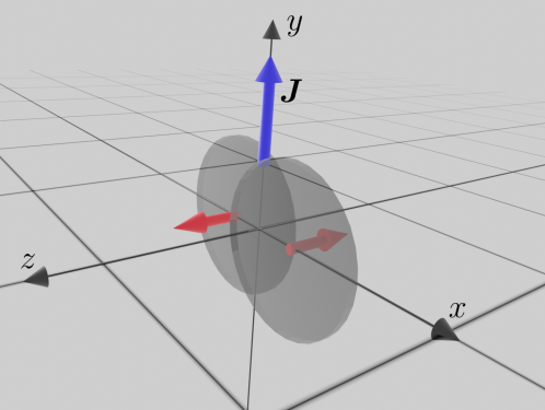
Figure 2: (Color online) Geometry of a relativistic heavy ion collision. The system is symmetric by rotation around $\textstyle\mathbf{J}$ by an angle $\pi$ and is invariant by reflection with respect to the reaction plane ($zx$ plane). Combining the two symmetries, the system is invariant by total reflection.

In general, one can expand the function $\zeta_{A}(x)$ at the freeze-out into multipolar components, thus separating the parity-conserving (odd $l$) from the parity-breaking (even $l$) terms:

$$\zeta_{A}(x)=\sum_{l=0}^{\infty}\sum_{m=-l}^{l}Z_{lm}(r)Y^{l}_{m}(\theta,\varphi)\,,$$ (12)

where $Y^{l}_{m}$ are the spherical harmonics. Correspondingly, the helicity function has a multipolar expansion in momentum space:

$$h_{\chi}({\bf p})=\sum_{l=0}^{\infty}\sum_{m=-l}^{l}H_{lm}(p)Y^{l}_{m}(\theta_{\bf p},\phi_{\bf p})$$ (13)

with parity-conserving odd $l$ terms and parity-breaking even $l$ terms. Note, however, that the relations between the $H_{lm}$ and the $Z_{lm}$ are not straightforward because of the non-trivial dependence on the coordinates of the Fermi-Dirac distribution in the equation  (10). Particularly, a coefficient $Z_{lm}$ in the eq. (12) cannot be reconstructed from the measurement of one coefficient $H_{lm}$ with the same couple of integers. In fact, many integers $(l,m)$ of $H_{lm}$ can contribute to one multipolar coefficient $Z_{LM}$ and vice-versa.

IV Parity violation and helicity azimuthal dependence

Local parity violation in the helicity spectrum can be established, in a model independent way, by studying the azimuthal dependence of, e.g. $\Lambda$ hyperon helicity in the transverse plane to verify the non-vanishing even $l$ terms in the expansion (13). Let us consider, for simplicity, particles emitted at midrapidity in a heavy ion collisions, i.e. with vanishing longitudinal momentum $p_{z}=0$; the momentum vector ${\bf p}$ is then only transverse and can be described by a magnitude $p_{T}$ and the azimuthal angle $\phi$ with respect to the reaction plane $y=0$ in figure 2. In this case, the expansion (13) becomes a single-variable Fourier expansion in the azimuthal angle $\phi$. The helicity function can be split into a parity preserving pseudo-scalar part $h_{P}$ and a parity breaking scalar part $h_{S}$. Taking into account the rotational symmetry $\phi\to\pi-\phi$ and their transformation properties under reflection $\phi\to\pi+\phi$, they can be written as:

$$h_{P}(p_{T},\phi) =\sum_{k}P_{k}(p_{T})\sin[(2k+1)\phi],$$ (14)

$$h_{S}(p_{T},\phi) =\sum_{k}S_{k}(p_{T})\cos[2k\phi].$$

The above forms are dictated by symmetry, hence they are completely general and model-independent. The models, amongst which the local equilibrium model with axial chemical potential, in principle predict the function (10) and, consequently, the momentum dependent coefficients of $P_{k}$ and $S_{k}$ in the (14).

The hydrodynamic polarization in eq.(7) does not break parity and does not contribute to $h_{S}$, but only to $h_{P}$. As we have emphasized, unlike for the $P_{k}$’s, the $S_{k}$’s average to zero over many events and suitable observables must be devised to detect them. For instance, by retaining only the leading harmonics in the (14), the helicity squared reads:

$$h^{2}({\bf p}_{T})=(S_{0}+P_{0}\sin\phi)^{2}=S_{0}^{2}+P_{0}^{2}\sin^{2}\phi+2S_{0}P_{0}\sin\phi$$ (15)

and, assuming that $S_{0}$ and $P_{0}$ are uncorrelated, being $\langle\langle S_{0}\rangle\rangle=0$ when averaging over many events, one has:

$$\langle\langle h^{2}({\bf p}_{T})\rangle\rangle=\langle\langle S_{0}^{2}\rangle\rangle+\langle\langle P_{0}^{2}\rangle\rangle\sin^{2}\phi\,.$$ (16)

The constant term $\langle\langle S_{0}^{2}\rangle\rangle$ is non-vanishing and, at least in principle, one could think of measuring it by fitting the $h^{2}(\phi)$ azimuthal function. However, since helicity can only be measured through the fluctuating angle between the momentum of the $\Lambda$ and the momentum of the decay proton in the $\Lambda$ rest frame, it would be hard to disentangle a mean value of the helicity squared from the fluctuation variance. Moreover, an accurate identification of the reaction plane is needed (not its orientation though) which might be difficult to achieve.

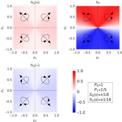
Figure 3: (Color online) Examples of the distributions of the scalar, parity-breaking, component of the helicity (left) and of the pseudoscalar component (right) in the transverse momentum plane. The contour plots show the profile of the helicity calculated with the Fourier expansion (14) and parameter values quoted in the right bottom corner. The parity-breaking component fluctuates on an event-by event basis with positive or negative values (left).

A better and definitely more realistic method is based on the measurement of the helicity-helicity angular correlation in the same event. Azimuthal polarization correlations have been proposed to detect the vortical structure of the hydrodynamic motion Pang et al. (2016) and we find here that they can be used to detect the chirality imbalance as well. Suppose that two (or more) hyperons are emitted in the same event at two different angles $\phi$ and $\phi+\Delta\phi$ and also suppose, for illustrative purpose, that there is no sizeable spin-spin two-particle correlation. Then, if

$$n({\bf p}_{T1},{\bf p}_{T2})=\frac{{\rm d}N}{d^{2}{\bf p}_{T1}{\rm d}^{2}{\bf p}_{T2}}$$

is the two-particle momentum spectrum, and $N$ its integral, we have:

$$\langle h_{1}h_{2}(\Delta\phi)\rangle=\frac{1}{N}\int{\rm d}^{2}{\bf p}_{T1}{\rm d}^{2}{\bf p}_{T2}\delta(\phi_{2}-\phi_{1}-\Delta\phi)\,h_{1}({\bf p}_{T1})h_{2}({\bf p}_{T2})n({\bf p}_{T1},{\bf p}_{T2})$$ (17)

which is expected to receive contributions from the parity violating terms. Neglecting momentum correlations and the azimuthal anisotropies of the spectrum, such as elliptic flow, which introduce just small corrections, and retaining only the leading harmonics just like in equation (15), one has:

$$\langle h_{1}h_{2}(\Delta\phi)\rangle \simeq\frac{1}{2\pi}\int_{0}^{2\pi}\mskip-3.0mu\mskip-3.0mu{\rm d}\phi\left(\bar{S}_{0}^{2}+\bar{P}_{0}^{2}\sin^{2}\phi\cos\Delta\phi\right)$$

$$=\bar{S}_{0}^{2}+\frac{1}{2}\bar{P}_{0}^{2}\cos\Delta\phi,$$

where the bar stands for transverse momentum average. The first term now survives the averaging over many events, so that a pedestal in the helicity-helicity azimuthal correlation function, like in eq. (16), signals a local parity violation. The constant, parity-breaking term, $S_{0}$ can be highlighted by integrating the equation (17) in $\Delta\phi$; it can be readily shown that, if momentum correlations are negligible as it was supposed for the equation (17):

$$\frac{1}{2\pi}\int_{0}^{2\pi}\mskip-3.0mu\mskip-3.0mu{\rm d}\Delta\phi\;\langle h_{1}h_{2}(\Delta\phi)\rangle=\bar{S}_{0}^{2}$$

It is important to stress that the correlation function (17), as well as other possible combinations of two helicities, does not require the identification of the reaction plane and can be measured by means of the angles between the $\Lambda$ momentum and the proton momentum in the $\Lambda$ rest frame.

While a non-vanishing value of the $\bar{S}_{0}^{2}$ is a clear signal of parity violation, one may wonders whether parity violation can be generated only by a genuine hot QCD-generated axial imbalance. Indeed, for the case of $\Lambda$, a possible source of background is the parity-violating polarization transfer in the weak $\Xi\to\Lambda$ decay. A quantitative assessment certainly goes beyond the scope of the present work; we just remark that secondary $\Lambda$s from $\Xi$ decays can be selected out through the displacement of their production point from the primary vertex of the collision, what makes this background not irreducible.

V Conclusions and outlook

To summarize, we have shown that the spin polarization vector of hyperons can be used to reveal local parity violation in hot QCD matter in relativistic heavy ion collisions. The helicity of $\Lambda$s acquires a term which is proportional to the fluctuating parity-breaking axial chemical potential, that we calculated in the linear approximation. To detect this contribution, we propose to measure the angular azimuthal correlation of the helicity of $\Lambda$ pairs in the same event through the measurement of the angle between the momentum of the hyperon and the momentum of the decay proton in its rest frame. For this purpose, a full quantitative study of the relation between the axial chemical potential distribution and the corresponding helicity pattern would be an important point of a future analysis.

Appendix A Calculation of the axial chemical contribution to the spin polarization vector

In this Appendix section we provide the detailed derivation of the contribution of the axial chemical potential to the polarization vector of a spin $1/2$ particles in a relativistic fluid at local thermodynamic equilibrium. We refer to the main letter for the notation.

The mean spin vector can be derived from the future time-like part of Wigner function of the emitted particle Becattini (2021):

$$S^{\mu}(p)=\frac{1}{2}\frac{\int_{\Sigma}{\rm d}\Sigma\cdot p\,{\rm tr}\left[\gamma^{\mu}\gamma^{5}W_{+}(x,p)\right]}{\int_{\Sigma}{\rm d}\Sigma\cdot p\,{\rm tr}\left[W_{+}(x,p)\right]},$$ (18)

where $\Sigma$ can be approximated as the freeze-out 3D hypersurface in Fig. 1. The Wigner function involves the effective hadronic fields, which are assumed to be free:

$$W_{+}(x,p)_{ab}=\frac{1}{(2\pi)^{4}}\int{\rm d}^{4}s\;{\rm e}^{-{\rm i}p\cdot s}{\rm Tr}({\widehat{\rho}}:{\overline{\Psi}}_{b}(x+s/2)\Psi_{a}(x-s/2):).$$ (19)

The density operator ${\widehat{\rho}}$ in the above equation must be fixed, in the Heisenberg representation. Therefore, in the hydrodynamic picture of the QCD plasma, it is assumed to be the local equilibrium density operator specified by the initial conditions Becattini et al. (2019), that is at the 3D hypersurface where the plasma is supposed to achieve local thermodynamic equilibrium ($\Sigma_{\mathrm{eq}}$ in Fig. 1):

$${\widehat{\rho}}=\frac{1}{Z}\exp\left[-\int_{\Sigma_{\mathrm{eq}}}{\rm d}\Sigma_{\mu}\left({\widehat{T}}^{\mu\nu}\beta_{\nu}-\zeta_{A}{\widehat{j}}_{A}^{\mu}\right)\right].$$ (20)

For the sake of simplicity, we have neglected all terms involving the conserved currents except for the axial current operator $\widehat{j}_{A}$ is the color-singlet axial current expressed in terms of the fundamental quark and gluon fields and includes the Chern-Simons current $\widehat{K}^{\mu}$ from anomaly Kharzeev (2010) so as to be a conserved one in the plasma phase. The exponent can be rewritten, by using the Gauss’ theorem (see Fig. 1):

$$\int_{\Sigma_{\mathrm{eq}}}{\rm d}\Sigma_{\mu}\left({\widehat{T}}^{\mu\nu}\beta_{\nu}-\zeta_{A}{\widehat{j}}_{A}^{\mu}\right)=\int_{\Sigma}{\rm d}\Sigma_{\mu}\left({\widehat{T}}^{\mu\nu}\beta_{\nu}-\zeta_{A}{\widehat{j}}_{A}^{\mu}\right)+\int_{\Omega}{\rm d}\Omega\left({\widehat{T}}^{\mu\nu}\partial_{\mu}\beta_{\nu}-{\widehat{j}}_{A}^{\mu}\partial_{\mu}\zeta_{A}-\zeta_{A}\partial_{\mu}{\widehat{j}}_{A}^{\mu}\right)$$ (21)

where $\Omega$ is the space-time region encompassed by the 3D hypersurfaces $\Sigma_{\mathrm{eq}}$ and $\Sigma=\Sigma_{\mathrm{FO}}\cup\sigma_{\pm}$ Becattini et al. (2019). The last term in the equation (21) is responsible for the dissipative corrections and includes a term with the divergence of the axial current which is quasi-vanishing in the chirally symmetric QGP phase (broken by quark masses). In the hydrodynamic approach, the local thermodynamic equilibrium term is dominant and one can obtain a good approximation by neglecting the second integral on the right hand side of (21):

$${\widehat{\rho}}\simeq{\widehat{\rho}}_{\textup{LE}}=\frac{1}{Z_{\textup{LE}}}\exp\left[-\int_{\Sigma}{\rm d}\Sigma_{\mu}\left({\widehat{T}}^{\mu\nu}\beta_{\nu}-\zeta_{A}{\widehat{j}}_{A}^{\mu}\right)\right].$$ (22)

The eq. (19) is indeed the mean value of the Wigner operator at the point $x$

$${\widehat{W}}(x,p)_{ab}=\frac{1}{(2\pi)^{4}}\int{\rm d}^{4}s\;{\rm e}^{-{\rm i}p\cdot s}:{\overline{\Psi}}_{b}(x+s/2)\Psi_{a}(x-s/2):$$

and, in the hydrodynamic limit of slowly varying $\beta(x)$ compared to the microscopic length scales, one can Taylor expand the $\beta$ field in (22) from $x$ and retain only the leading term:

$${\rm Tr}({\widehat{\rho}}_{\textup{LE}}{\widehat{W}}(x,p))\simeq\frac{1}{Z_{\textup{LE}}}{\rm Tr}\left({\widehat{W}}(x,p)\exp\left[-\beta(x)\cdot{\widehat{P}}+\int_{\Sigma}{\rm d}\Sigma_{\rho}\;\zeta_{A}{\widehat{j}}_{A}^{\rho}\right]\right),$$ (23)

where ${\widehat{P}}$ is the total four-momentum. The term involving the axial current term is supposedly small compared to the first term, hence one can expand the exponential in the (23) with the formula:

$${\rm e}^{{\widehat{A}}+{\widehat{B}}}={\rm e}^{{\widehat{A}}}+\int_{0}^{1}{\rm d}z\,{\rm e}^{z{\widehat{A}}}\,{\widehat{B}}\,{\rm e}^{-z{\widehat{A}}}\,{\rm e}^{{\widehat{A}}}+\cdots,$$

where:

$${\widehat{A}}=-\beta(x)\cdot{\widehat{P}},\quad{\widehat{B}}=\int_{\Sigma}{\rm d}\Sigma_{\rho}\;\zeta_{A}{\widehat{j}}_{A}^{\rho}.$$

Therefore, the response of the thermal expectation value of Wigner operator to the axial current term ${\widehat{B}}$ at local equilibrium is obtained by the previous expansion and is given by, for the particle term:

$$\langle{\widehat{W}}_{+}(x,p)\rangle_{\textup{LE}}\simeq\langle{\widehat{W}}_{+}(x,p)\rangle_{\beta(x)}+\Delta W_{+}(x,p)$$ (24)

with

$$\Delta W_{+}(x,p)=\int_{\Sigma}{\rm d}\Sigma_{\rho}(y)\;\zeta_{A}(y)\int_{0}^{1}{\rm d}z\;\langle\widehat{W}_{+}(x,p)\widehat{j}_{A}^{\rho}(y+{\rm i}z\beta(x))\rangle_{c,\beta(x)},$$ (25)

where the symbol $\langle\cdots\rangle_{\beta(x)}$ denotes thermal averages with the density operator

$${\widehat{\rho}}_{0}=\frac{1}{Z}\exp[-\beta(x)\cdot{\widehat{P}}]$$

i.e. the familiar homogeneous global equilibrium density operator in the grand-canonical ensemble. The subscript $c$ on the thermal average in (25) signifies the connected part of the correlator, that is, for the simplest case of two operators:

$$\langle\widehat{O}_{1}\widehat{O}_{2}\rangle_{c}\equiv\langle\widehat{O}_{1}\widehat{O}_{2}\rangle-\langle\widehat{O}_{1}\rangle\langle\widehat{O}_{2}\rangle.$$

The color-singlet axial current operator can be decomposed on the multi-hadronic Hilbert space basis and can be written as a combination of creation and annihilation operators Weinberg (2005):

$${\widehat{j}}_{A}^{\mu}(x)= \sum_{\begin{subarray}{c}N=0\\ M=0\end{subarray}}^{\infty}\sum_{\begin{subarray}{c}j_{1},\dots,j_{N}\\ k_{1},\dots,k_{M}\end{subarray}}\int\frac{{\rm d}^{3}\textrm{q}^{\prime}_{1}}{2\varepsilon^{\prime}_{1}}\cdots\int\frac{{\rm d}^{3}\textrm{q}^{\prime}_{N}}{2\varepsilon^{\prime}_{N}}\int\frac{{\rm d}^{3}\textrm{q}_{1}}{2\varepsilon_{1}}\cdots\int\frac{{\rm d}^{3}\textrm{q}_{M}}{2\varepsilon_{M}}$$

$$\times\widehat{a}^{\dagger}_{j_{1}}(q^{\prime}_{1})\cdots\widehat{a}^{\dagger}_{j_{N}}(q^{\prime}_{N})\widehat{a}_{k_{1}}(q_{1})\cdots\widehat{a}_{k_{M}}(q_{M})J^{\mu}(q^{\prime},q,x)^{j_{1},\dots,k_{M}}$$

where the indices $j_{l}$ and $k_{l}$ label the various hadronic species and the spin indices of the creation and annihilation operators have been omitted. Each function $J(p^{\prime},p,x)$ can be obtained by forming suitable multi-hadronic matrix elements. In the formula (25), most of the above terms vanish and the predominant contribution is given by the term with two particles of the same species $h$ as specified by the Wigner operator, which is made of hadronic fields. Specifically, the predominant term reads (with spin indices):

$$\sum_{\sigma,\sigma^{\prime}}\int\frac{{\rm d}^{3}\textrm{q}^{\prime}}{2\varepsilon_{q^{\prime}}}\int\frac{{\rm d}^{3}\textrm{q}}{2\varepsilon_{q}}\;\widehat{a}^{\dagger}_{h}(p^{\prime})_{\sigma^{\prime}}\widehat{a}_{h}(q)_{\sigma}J(q,q^{\prime},x)_{\sigma,\sigma^{\prime}}^{hh}$$ (26)

and the integrand function can be obtained by taking the following matrix element of the axial current:

$$J^{\mu}(q,q^{\prime},x)_{\sigma,\sigma^{\prime}}^{hh}=\langle 0|\widehat{a}_{\sigma^{\prime}}(q^{\prime}){\widehat{j}}_{A}^{\mu}(x)\widehat{a}_{\sigma}^{\dagger}(q)|0\rangle=\langle q^{\prime},\sigma^{\prime}|{\widehat{j}}_{A}^{\mu}(x)|q,\sigma\rangle$$ (27)

where creation and annihilation operators are covariantly normalized:

$$[\widehat{a}_{\sigma}(q),\widehat{a}_{\sigma^{\prime}}^{\dagger}(q^{\prime})]_{\pm}=2\varepsilon\,\delta_{\sigma\sigma^{\prime}}\delta^{3}(\mathchoice{\mbox{\boldmath$\displaystyle\mathbf{q}$}}{\mbox{\boldmath$\textstyle\mathbf{q}$}}{\mbox{\boldmath$\scriptstyle\mathbf{q}$}}{\mbox{\boldmath$\scriptscriptstyle\mathbf{q}$}}-\mathchoice{\mbox{\boldmath$\displaystyle\mathbf{q}$}}{\mbox{\boldmath$\textstyle\mathbf{q}$}}{\mbox{\boldmath$\scriptstyle\mathbf{q}$}}{\mbox{\boldmath$\scriptscriptstyle\mathbf{q}$}}^{\prime}).$$

The matrix element of the axial current on two spin 1/2 hadronic states has a well-known form which is dictated by Poincaré symmetry and Dirac equation:

$$\langle q^{\prime},\sigma^{\prime}|{\widehat{j}}_{A}^{\mu}(x)|q,\sigma\rangle=\frac{1}{(2\pi)^{3}}\;{\rm e}^{{\rm i}Q\cdot x}\bar{u}_{\sigma^{\prime}}(q^{\prime})\left[G_{A1}(Q^{2})\gamma^{\mu}\gamma^{5}+\frac{Q^{\mu}}{2m_{h}}G_{A2}(Q^{2})\gamma^{5}\right]u_{\sigma}(q)$$ (28)

with $Q=(q^{\prime}-q)$ and $u(q)$ are the spinors of the hadron normalized so as to:

$$\bar{u}_{\sigma}(k)u_{\sigma^{\prime}}(k)=2m_{h}\,\delta_{\sigma\sigma^{\prime}},\qquad\bar{v}_{\sigma}(k)v_{\sigma^{\prime}}(k)=-2m_{h}\,\delta_{\sigma\sigma^{\prime}}\,.$$

The axial form factors $G_{A1}(Q^{2})$ and $G_{A2}(Q^{2})$ depend on the flavour-space transformation properties of the axial current ${\widehat{j}}_{A}$, that is whether ${\widehat{j}}_{A}$ includes the strange quark term and to what extent.

Altogether, the relevant part of the axial current operator in (25) is obtained by plugging the (28) and (27) into the (26):

$$\widehat{j}_{A}^{\rho}(y+{\rm i}z\beta)\rightarrow\widehat{j}_{A,h}^{\rho}(y+{\rm i}z\beta)=\frac{1}{(2\pi)^{3}}\sum_{\sigma,\sigma^{\prime}} \int\frac{{\rm d}^{3}\textrm{q}^{\prime}}{2\varepsilon_{q^{\prime}}}\int\frac{{\rm d}^{3}\textrm{q}}{2\varepsilon_{q}}\;\widehat{a}^{\dagger}_{h}(q^{\prime})_{\sigma^{\prime}}\widehat{a}_{h}(q)_{\sigma}{\rm e}^{{\rm i}Q\cdot y-zt\cdot\beta}$$ (29)

$$\times\bar{u}_{\sigma^{\prime}}(q^{\prime})\left[G_{A1}(Q^{2})\gamma^{\mu}\gamma^{5}+\frac{Q^{\mu}}{2m_{h}}G_{A2}(Q^{2})\gamma^{5}\right]u_{\sigma}(q).$$

We are now in a position to work out the (25). The Wigner operator can be expanded by using the normal mode expansion of the Dirac field:

$$\Psi(x)=\sum_{\sigma=1}^{2}\frac{1}{(2\pi)^{3/2}}\int\frac{{\rm d}^{3}{\rm k}}{2\varepsilon_{k}}\left[u_{\sigma}(k){\rm e}^{-{\rm i}k\cdot x}\widehat{a}_{h}(k)_{\sigma}+v_{\sigma}(k){\rm e}^{{\rm i}k\cdot x}\widehat{b}^{\dagger}_{h}(k)_{\sigma}\right]$$

and retaining only the particle operators $\widehat{a}_{h}$ and $\widehat{a}^{\dagger}_{h}$:

$$\widehat{W}_{+}(x,p)_{ab}=\frac{1}{(2\pi)^{3}}\sum_{\tau,\tau^{\prime}}\int\frac{{\rm d}^{3}{\rm k}}{2\varepsilon_{k}}\int\frac{{\rm d}^{3}{\rm k}^{\prime}}{2\varepsilon_{k^{\prime}}}\delta^{4}(p-(k+k^{\prime})/2){\rm e}^{-{\rm i}x\cdot(k^{\prime}-k)}u_{\tau^{\prime}}(k^{\prime})_{a}\bar{u}_{\tau}(k)_{b}\widehat{a}^{\dagger}_{h}(k)_{\tau}\widehat{a}_{h}(k^{\prime})_{\tau^{\prime}},$$ (30)

while for the axial current the equation (29) is employed. From now on we omit the subscript $h$ as only one hadronic species is involved.

It turns out that the correlator $\Delta W_{+}(x,p)_{ab}$ in the eq. (25) involves the thermal expectation values between four creation and annihilation operators where the first two operators come from the Wigner operator in the eq.  (30) and the remaining two operators from the axial current operator in the eq. (29). Thanks to the thermal Wick theorem, a four-operator thermal expectation value can be reduced to the product of two-operator thermal expectation values as follows:

$$\langle\widehat{a}^{\dagger}_{1}\widehat{a}_{2}\widehat{a}^{\dagger}_{3}\widehat{a}_{4}\rangle_{c}=\langle\widehat{a}^{\dagger}_{1}\widehat{a}_{2}\widehat{a}^{\dagger}_{3}\widehat{a}_{4}\rangle-\langle\widehat{a}^{\dagger}_{1}\widehat{a}_{2}\rangle\langle\widehat{a}^{\dagger}_{3}\widehat{a}_{4}\rangle=\langle\widehat{a}^{\dagger}_{1}\widehat{a}_{4}\rangle\langle\widehat{a}_{2}\widehat{a}^{\dagger}_{3}\rangle\;.$$

The two-operator thermal expectation values for non-interacting fields with the homogeneous grand-canonical ensemble operator ${\widehat{\rho}}_{0}$ are given by:

$$\begin{split}\langle\widehat{a}^{\dagger}_{\tau}(k)\widehat{a}_{\sigma}(q)\rangle_{\beta(x)}=&\delta_{\tau\sigma}2\varepsilon_{q}\delta^{3}(\mathchoice{\mbox{\boldmath$\displaystyle\mathbf{k}$}}{\mbox{\boldmath$\textstyle\mathbf{k}$}}{\mbox{\boldmath$\scriptstyle\mathbf{k}$}}{\mbox{\boldmath$\scriptscriptstyle\mathbf{k}$}}-\mathchoice{\mbox{\boldmath$\displaystyle\mathbf{q}$}}{\mbox{\boldmath$\textstyle\mathbf{q}$}}{\mbox{\boldmath$\scriptstyle\mathbf{q}$}}{\mbox{\boldmath$\scriptscriptstyle\mathbf{q}$}})n_{\textup{F}}(k,x),\\ \langle\widehat{a}_{\tau^{\prime}}(k^{\prime})\widehat{a}^{\dagger}_{\sigma^{\prime}}(q^{\prime})\rangle_{\beta(x)}=&\delta_{\tau^{\prime}\sigma^{\prime}}2\varepsilon_{q^{\prime}}\delta^{3}(\mathchoice{\mbox{\boldmath$\displaystyle\mathbf{k\bm{{}^{\prime}}}$}}{\mbox{\boldmath$\textstyle\mathbf{k\bm{{}^{\prime}}}$}}{\mbox{\boldmath$\scriptstyle\mathbf{k\bm{{}^{\prime}}}$}}{\mbox{\boldmath$\scriptscriptstyle\mathbf{k\bm{{}^{\prime}}}$}}-\mathchoice{\mbox{\boldmath$\displaystyle\mathbf{q\bm{{}^{\prime}}}$}}{\mbox{\boldmath$\textstyle\mathbf{q\bm{{}^{\prime}}}$}}{\mbox{\boldmath$\scriptstyle\mathbf{q\bm{{}^{\prime}}}$}}{\mbox{\boldmath$\scriptscriptstyle\mathbf{q\bm{{}^{\prime}}}$}})(1-n_{\textup{F}}(k^{\prime},x)),\end{split}$$ (31)

where $n_{\textup{F}}$ is the covariant Fermi-Dirac distribution function

$$n_{\textup{F}}(k,x)=\frac{1}{{\rm e}^{\beta(x)\cdot k}+1}.$$

All other combinations have vanishing expectation values.

By using the (31), after some simple calculation, both terms on the right hand side of the equation (24) can be worked out:

$$\langle{\widehat{W}}_{+}(x,p)\rangle_{\beta(x)}=\left(m+\gamma^{\mu}p_{\mu}\right)\delta(p^{2}-m^{2})\theta(p_{0})\frac{1}{(2\pi)^{3}}n_{\textup{F}}\left(p\right),$$ (32)

and:

$$\Delta W(x,p)_{+ab}= \int_{\Sigma}{\rm d}\Sigma_{\rho}(y)\;\zeta_{A}(y)\int_{0}^{1}{\rm d}z\;\frac{1}{(2\pi)^{6}}\int\frac{{\rm d}^{3}{\rm k}\,{\rm d}^{3}{\rm k}^{\prime}}{4\varepsilon_{k}\varepsilon_{k^{\prime}}}\;\delta^{4}\left(p-\frac{k+k^{\prime}}{2}\right)n_{\textup{F}}(k,x)(1-n_{\textup{F}}(k^{\prime},x))$$ (33)

$$\times{\mathcal{A}}^{\rho}(k,k^{\prime})_{ab}\,{\rm e}^{{\rm i}(k-k^{\prime})\cdot(x-y)}{\rm e}^{z(k-k^{\prime})\cdot\beta(x)}$$

where we defined:

$${\mathcal{A}}^{\rho}(k,k^{\prime})\equiv(\not{k}^{\prime}+m)\left[G_{A1}\left(Q^{2}\right)\gamma^{\rho}\gamma^{5}+\frac{{k^{\prime}}^{\rho}-k^{\rho}}{2m}G_{A2}\left(Q^{2}\right)\gamma^{5}\right](\not{k}+m),$$

where now $Q=(k^{\prime}-k)$ because of the (31), and use has been made of the known relation:

$$\sum_{\sigma}u_{\sigma}(k)\bar{u}_{\sigma}(k)=\not{k}+m.$$

We can now work out an approximated expression of the mean spin vector due to the axial chemical potential. By replacing the Wigner function in the eq. (18) with its local equilibrium approximation (24), and making use of the (32) taking into account the known traces of the $\gamma$ matrices, we are left with:

$$S^{\mu}_{\chi}(p)=\frac{1}{2}\frac{\int_{\Sigma}{\rm d}\Sigma\cdot p\;{\rm tr}\left[\gamma^{\mu}\gamma^{5}\Delta W_{+}(x,p)\right]}{\int_{\Sigma}{\rm d}\Sigma\cdot p\;{\rm tr}\left[\langle\widehat{W}_{+}(x,p)\rangle_{\beta(x)}+\Delta W_{+}(x,p)\right]}$$ (34)

as the term due to eq. (32) in the numerator gives vanishing contribution. To proceed, we need to calculate some traces:

$$\begin{split}{\rm tr}&\left(\not{p}+m\right)=4m\\ {\rm tr}&\left[(\not{k}^{\prime}+m)\gamma^{\rho}\gamma^{5}(\not{k}+m)\right]=0,\\ {\rm tr}&\left[(\not{k}^{\prime}+m)\gamma^{5}(\not{k}+m)\right]=0,\\ {\rm tr}&\left[\gamma^{\mu}\gamma^{5}(\not{k}^{\prime}+m)\gamma^{5}(\not{k}+m)\right]=-4m({k^{\prime}}^{\mu}-k^{\mu})\\ {\rm tr}&\left[\gamma^{\mu}\gamma^{5}(\not{k}^{\prime}+m)\gamma^{\rho}\gamma^{5}(\not{k}+m)\right]=-4\Big{(}\eta^{\mu\rho}(m^{2}+k\cdot k^{\prime})-k^{\rho}{k^{\prime}}^{\mu}-k^{\mu}{k^{\prime}}^{\rho}\Big{)}.\end{split}$$

By plugging the equations (32) and (33) into the (34) and using the above trace formulae, the following expression is found for the mean spin vector:

$$\begin{split}S^{\mu}_{\chi}(p)=&-\frac{2}{\mathcal{D}}\int_{\Sigma}{\rm d}\Sigma(x)\cdot p\int_{\Sigma}{\rm d}\Sigma_{\rho}(y)\;\zeta_{A}(y)\int_{0}^{1}\frac{{\rm d}z}{(2\pi)^{6}}\int\frac{{\rm d}^{3}{\rm k}}{2\varepsilon_{k}}\int\frac{{\rm d}^{3}{\rm k}^{\prime}}{2\varepsilon_{k^{\prime}}}\delta^{4}\left(p-\frac{k+k^{\prime}}{2}\right)\\ &\times{\mathcal{B}}^{\mu\rho}(k,k^{\prime})n_{\textup{F}}(k,x)(1-n_{\textup{F}}(k^{\prime},x)){\rm e}^{{\rm i}(k-k^{\prime})\cdot(x-y)}{\rm e}^{z(k-k^{\prime})\cdot\beta(x)},\end{split}$$ (35)

where:

$${\mathcal{B}}^{\mu\rho}(k,k^{\prime})\equiv G_{A1}(Q^{2})\left[\eta^{\mu\rho}(m^{2}+k\cdot k^{\prime})-k^{\rho}{k^{\prime}}^{\mu}-k^{\mu}{k^{\prime}}^{\rho}\right]+\frac{1}{2}G_{A2}\left(Q^{2}\right)({k^{\prime}}^{\mu}-k^{\mu})({k^{\prime}}^{\rho}-k^{\rho})$$ (36)

and ${\mathcal{D}}$ is the denominator in the leading order approximation:

$${\mathcal{D}}=\frac{4m}{(2\pi)^{3}}\int_{\Sigma}{\rm d}\Sigma\cdot p\;\delta(p^{2}-m^{2})\theta(p_{0})n_{\textup{F}}(p).$$ (37)

The (35) is a double integral in $x,y$ which can be recast as:

$$S^{\mu}_{\chi}(p)=-\frac{2}{\mathcal{D}}\int_{\Sigma}{\rm d}\Sigma(x)\cdot p\;\int_{\Sigma}{\rm d}\Sigma_{\rho}(y)\zeta_{A}(y)\;G^{\mu\rho}(\beta(x),x-y)$$

where the function $G$ results from the integration in ${\rm k},{\rm k}^{\prime},z$. The function $G$ decays on microscopic length scales as a function of its argument $x-y$ whereas the function $\zeta_{A}$ supposedly varies significantly over a longer length scale, in the hydrodynamic picture. Therefore, one can obtain a good approximation of the above expression by replacing $\zeta_{A}(y)$ with $\zeta_{A}(x)$ and taking it out of the $y$ integral. By doing so, only an exponential is left to be integrated in $y$ in the eq. (35):

$$\int_{\Sigma}{\rm d}\Sigma_{\rho}(y)\;\zeta_{A}(y){\rm e}^{{\rm i}(k-k^{\prime})\cdot(x-y)}\simeq\zeta_{A}(x)\int_{\Sigma}{\rm d}\Sigma_{\rho}(y)\;{\rm e}^{{\rm i}(k-k^{\prime})\cdot(x-y)}.$$

To evaluate the integral over the hypersurface $\Sigma$, one can take advantage of the Gauss theorem. By denoting with $\Omega_{\textup{B}}$ the space-time region encompassed by the 3D hypersurfaces $\Sigma_{\mathrm{FO}}$ and $\Sigma_{B}$ which is the hyperplane region connecting the $\Sigma_{\textup{FO}}$ boundaries (see Fig. 1):

$$\int_{\Sigma}{\rm d}\Sigma_{\rho}(y)\;{\rm e}^{{\rm i}(k-k^{\prime})\cdot(x-y)}=\int_{\sigma_{\pm}}{\rm d}\Sigma_{\rho}(y)\;{\rm e}^{{\rm i}(k-k^{\prime})\cdot(x-y)}+\int_{\Sigma_{\textup{B}}}{\rm d}\Sigma_{\rho}(y)\;{\rm e}^{{\rm i}(k-k^{\prime})\cdot(x-y)}-{\rm i}(k-k^{\prime})_{\rho}\int_{\Omega_{\textup{B}}}{\rm d}^{4}y\,{\rm e}^{{\rm i}(k-k^{\prime})\cdot(x-y)}.$$

The contribution afrom the hyperbolic branches $\sigma_{\pm}$, which have not even entered the plasma phase (see Fig. 1), can be neglected altogether, especially at high energy. The 3D hypersurface $\Sigma_{\textup{B}}$ is a subset of a hyperplane parallel to $t=0$ in the center-of-mass frame (see Fig. 1), thus ${\rm d}\Sigma_{\rho}=\hat{t}_{\rho}{\rm d}^{3}{\mathrm{y}}=\delta^{0}_{\rho}{\rm d}^{3}{\mathrm{y}}$. If it is large enough, one can approximate it with a Dirac $\delta$:

$$\int_{\Sigma_{\textup{B}}}{\rm d}\Sigma_{\rho}(y)\,{\rm e}^{{\rm i}(k-k^{\prime})\cdot(x-y)}=\hat{t}_{\rho}\int{\rm d}^{3}y\,{\rm e}^{{\rm i}(k-k^{\prime})\cdot(x-y)}\simeq\hat{t}_{\rho}(2\pi)^{3}\delta^{3}(\mathchoice{\mbox{\boldmath$\displaystyle\mathbf{k}$}}{\mbox{\boldmath$\textstyle\mathbf{k}$}}{\mbox{\boldmath$\scriptstyle\mathbf{k}$}}{\mbox{\boldmath$\scriptscriptstyle\mathbf{k}$}}-\mathchoice{\mbox{\boldmath$\displaystyle\mathbf{k\bm{{}^{\prime}}}$}}{\mbox{\boldmath$\textstyle\mathbf{k\bm{{}^{\prime}}}$}}{\mbox{\boldmath$\scriptstyle\mathbf{k\bm{{}^{\prime}}}$}}{\mbox{\boldmath$\scriptscriptstyle\mathbf{k\bm{{}^{\prime}}}$}}).$$

Likewise, in the same approximation, the integral over the region $\Omega_{\textup{B}}$ multiplied by $(k-k^{\prime})$ vanishes and one is finally left with the approximation:

$$\int_{\Sigma}{\rm d}\Sigma_{\rho}(y)\zeta_{A}(y){\rm e}^{{\rm i}(k-k^{\prime})\cdot(x-y)}\simeq\zeta_{A}(x)\hat{t}_{\rho}(2\pi)^{3}\delta^{3}(\mathchoice{\mbox{\boldmath$\displaystyle\mathbf{k}$}}{\mbox{\boldmath$\textstyle\mathbf{k}$}}{\mbox{\boldmath$\scriptstyle\mathbf{k}$}}{\mbox{\boldmath$\scriptscriptstyle\mathbf{k}$}}-\mathchoice{\mbox{\boldmath$\displaystyle\mathbf{k\bm{{}^{\prime}}}$}}{\mbox{\boldmath$\textstyle\mathbf{k\bm{{}^{\prime}}}$}}{\mbox{\boldmath$\scriptstyle\mathbf{k\bm{{}^{\prime}}}$}}{\mbox{\boldmath$\scriptscriptstyle\mathbf{k\bm{{}^{\prime}}}$}}).$$ (38)

With ${\mathbf{k}}={\mathbf{k}}^{\prime}$, being $k$ on-shell, we have $k=k^{\prime}$ and $Q=(k^{\prime}-k)=0$. Therefore, the equation (36) simplifies to:

$${\mathcal{B}}^{\mu\rho}(k,k)=2g_{h}\left(\eta^{\mu\rho}m^{2}-k^{\rho}k^{\mu}\right),$$

where $g_{h}=G_{A1}(0)$ is the axial charge, that is the matrix element (28) at zero momentum transfer. With the approximation (38) we can readily integrate the expression (35) in $k^{\prime}$ and we obtain

$$S^{\mu}_{\chi}(p)\simeq-\frac{2g_{h}}{\mathcal{D}}\int_{\Sigma}{\rm d}\Sigma(x)\cdot p\;\zeta_{A}(x)\int_{0}^{1}\frac{{\rm d}z}{(2\pi)^{3}}\int\frac{{\rm d}^{3}{\rm k}}{2\varepsilon_{k}}\frac{1}{2\varepsilon_{k}}\delta^{4}\left(p-k\right)2\left[\hat{t}^{\mu}m^{2}-\varepsilon_{k}k^{\mu}\right]n_{\textup{F}}(k,x)(1-n_{\textup{F}}(k,x)).$$

Now, the dependence on $z$ is gone and the integration in $z$ is thus trivial. Moreover:

$$\int\frac{{\rm d}^{3}{\rm k}}{2\varepsilon_{k}}\delta^{4}(p-k)f^{\mu}(k)=\int{\rm d}^{4}k\;\delta(k^{2}-m^{2})\theta(k_{0})\delta^{4}(k-p)f^{\mu}(k)=\theta(p_{0})\delta(p^{2}-m^{2})f^{\mu}(p),$$

where

$$f^{\mu}(k)=\frac{\hat{t}^{\mu}m^{2}-\varepsilon_{k}k^{\mu}}{\varepsilon_{k}}n_{\textup{F}}(k,x)(1-n_{\textup{F}}(k,x)).$$

By using the previous results and replacing the denominator (37), the final expression of the mean spin vector, at the leading order in the axial chemical potential, is obtained:

$$S^{\mu}_{\chi}(p)=\frac{g_{h}}{2}\frac{\int_{\Sigma}{\rm d}\Sigma(x)\cdot p\;\zeta_{A}(x)n_{\textup{F}}(p,x)\left(1-n_{\textup{F}}(p,x)\right)\delta(p^{2}-m^{2})\theta(p_{0})}{\int_{\Sigma}{\rm d}\Sigma(x)\cdot p\;n_{\textup{F}}(p,x)\delta(p^{2}-m^{2})\theta(p_{0})}\frac{\varepsilon p^{\mu}-m^{2}\hat{t}^{\mu}}{m\varepsilon}.$$

Since the integration over the hypersurface puts the momentum $p$ on-shell Becattini (2021), the delta functions $\delta(p^{2}-m^{2})$ give rise to an infinite constant and cancel out in the ratio, while $\theta(p_{0})$ becomes redundant. Therefore, the mean spin vector induced by chiral imbalance, at the leading order in the axial chemical potential, is:

$$\begin{split}S^{\mu}_{\chi}(p)=&\frac{g_{h}}{2}\frac{\int_{\Sigma}{\rm d}\Sigma\cdot p\;\zeta_{A}n_{\textup{F}}\left(1-n_{\textup{F}}\right)}{\int_{\Sigma}{\rm d}\Sigma\cdot p\;n_{\textup{F}}}\frac{\varepsilon p^{\mu}-m^{2}\hat{t}^{\mu}}{m\varepsilon}\end{split}$$

where the arguments have been omitted.