Why resampling outperforms reweighting for correcting sampling bias with stochastic gradients

Abstract

A data set sampled from a certain population is biased if the subgroups of the population are sampled at proportions that are significantly different from their underlying proportions. Training machine learning models on biased data sets requires correction techniques to compensate for the bias. We consider two commonly-used techniques, resampling and reweighting, that rebalance the proportions of the subgroups to maintain the desired objective function. Though statistically equivalent, it has been observed that resampling outperforms reweighting when combined with stochastic gradient algorithms. By analyzing illustrative examples, we explain the reason behind this phenomenon using tools from dynamical stability and stochastic asymptotics. We also present experiments from regression, classification, and off-policy prediction to demonstrate that this is a general phenomenon. We argue that it is imperative to consider the objective function design and the optimization algorithm together while addressing the sampling bias.

1 Introduction

A data set sampled from a certain population is called biased if the subgroups of the population are sampled at proportions that are significantly different from their underlying population proportions. Applying machine learning algorithms naively to biased training data can raise serious concerns and lead to controversial results (Sweeney, 2013; Kay et al., 2015; Menon et al., 2020). In many domains such as demographic surveys, fraud detection, identification of rare diseases, and natural disasters prediction, a model trained from biased data tends to favor oversampled subgroups by achieving high accuracy there while sacrificing the performance on undersampled subgroups. Although one can improve by diversifying and balancing during the data collection process, it is often hard or impossible to eliminate the sampling bias due to historical and operational issues.

In order to mitigate the biases and discriminations against the undersampled subgroups, a common technique is to preprocess the data set by compensating the mismatch between population proportion and the sampling proportion. Among various approaches, two commonly-used choices are reweighting and resampling. In reweighting, one multiplies each sample with a ratio equal to its population proportion over its sampling proportion. In resampling, on the other hand, one corrects the proportion mismatch by either generating new samples for the undersampled subgroups or selecting a subset of samples for the oversampled subgroups. Both methods result in statistically equivalent models in terms of the loss function (see details in Section 2). However, it has been observed in practice that resampling often outperforms reweighting significantly, such as boosting algorithms in classification (Galar et al., 2011; Seiffert et al., 2008), off-policy prediction in reinforcement learning (Schlegel et al., 2019) and so on. The obvious question is why.

Main contributions.

Our main contribution is to provide an answer to this question: resampling outperforms reweighting because of the stochastic gradient-type algorithms used for training. To the best of our knowledge, our explanation is the first theoretical quantitative analysis for this phenomenon. With stochastic gradient descent (SGD) being the dominant method for model training, our analysis is based on some recent developments for understanding SGD. We show via simple and explicitly analyzable examples why resampling generates expected results while reweighting performs undesirably. Our theoretical analysis is based on two points of view, one from the dynamical stability perspective and the other from stochastic asymptotics.

In addition to the theoretical analysis, we present experimental examples from three distinct categories (classification, regression, and off-policy prediction) to demonstrate that resampling outperforms reweighting in practice. This empirical study illustrates that this is a quite general phenomenon when models are trained using stochastic gradient type algorithms.

Our theoretical analysis and experiments show clearly that adjusting only the loss functions is not sufficient for fixing the biased data problem. The output can be disastrous if one overlooks the optimization algorithm used in the training. In fact, recent understanding has shown that objective function design and optimization algorithm are closely related, for example optimization algorithms such as SGD play a key role in the generalizability of deep neural networks. Therefore in order to address the biased data issue, we advocate for considering data, model, and optimization as an integrated system.

Related work.

In a broader scope, resampling and reweighting can be considered as instances of preprocessing the training data to tackle biases of machine learning algorithms. Though there are many well-developed resampling (Mani & Zhang, 2003; He & Garcia, 2009; Maciejewski & Stefanowski, 2011) and reweighting (Kumar et al., 2010; Malisiewicz et al., 2011; Chang et al., 2017) techniques, we only focus on the reweighting approaches that do not change the optimization problem. It has been well-known that training algorithms using disparate data can lead to algorithmic discrimination (Bolukbasi et al., 2016; Caliskan et al., 2017), and over the years there have been growing efforts to mitigate such biases, for example see (Amini et al., 2019; Kamiran & Calders, 2012; Calmon et al., 2017; Zhao et al., 2019; López et al., 2013). We also refer to (Guo et al., 2017; He & Ma, 2013; Krawczyk, 2016) for a comprehensive review of this growing research field.

Our approaches for understanding the dynamics of resampling and reweighting under SGD are based on tools from numerical analysis for stochastic systems. Connections between numerical analysis and stochastic algorithms have been rapidly developing in recent years. The dynamical stability perspective has been used in (Wu et al., 2018) to show the impact of learning rate and batch size in minima selection. The stochastic differential equations (SDE) approach for approximating stochastic optimization methods can be traced in the line of work (Li et al., 2017; 2019; Rotskoff & Vanden-Eijnden, 2018; Shi et al., 2019), just to mention a few.

2 Problem setup

Let us consider a population that is comprised of two different groups, where a proportion $a_{1}$ of the population belongs to the first group, and the rest with the proportion $a_{2}=1-a_{1}$ belongs to the second (i.e., $a_{1},a_{2}>0$ and $a_{1}+a_{2}=1$). In what follows, we shall call $a_{1}$ and $a_{2}$ the population proportions. Consider an optimization problem for this population over a parameter $\theta$. For simplicity, we assume that each individual from the first group experiences a loss function $V_{1}(\theta)$, while each individual from the second group has a loss function of type $V_{2}(\theta)$. Here the loss function $V_{1}(\theta)$ is assumed to be identical across all members of the first group and the same for $V_{2}(\theta)$ across the second group, however it is possible to extend the formulation to allow for loss function variation within each group. Based on this setup, a minimization problem over the whole population is to find

$$\theta^{*}=\operatorname*{arg\,min}_{\theta}V(\theta),\quad\text{ where }~{}V(\theta)\equiv a_{1}V_{1}(\theta)+a_{2}V_{2}(\theta).$$ (1)

For a given set $\Omega$ of $N$ individuals sampled uniformly from the population, the empirical minimization problem is

$$\theta^{*}=\operatorname*{arg\,min}_{\theta}\frac{1}{N}\sum_{r\in\Omega}V_{i_{r}}(\theta),$$ (2)

where $i_{r}\in\{1,2\}$ denotes which group an individual $r$ belongs to. When $N$ grows, the empirical loss in (2) is consistent with the population loss in (1) as there are approximately $a_{1}$ fraction of samples from the first group and $a_{2}$ fraction of samples from the second.

However, the sampling can be far from uniformly random in reality. Let $n_{1}$ and $n_{2}$ with $n_{1}+n_{2}=N$ denote the number of samples from the first and the second group, respectively. It is convenient to define $f_{i},i=1,2$ as the sampling proportions for each group, i.e., $f_{1}=n_{1}/N$ and $f_{2}=n_{2}/N$ with $f_{1}+f_{2}=1$. The data set is biased when the sampling proportions $f_{1}$ and $f_{2}$ are different from the population proportions $a_{1}$ and $a_{2}$. In such a case, the empirical loss is $f_{1}V_{1}(\theta)+f_{2}V_{2}(\theta)$, which is clearly wrong when compared with (1).

Let us consider two basic strategies to adjust the model: reweighting and resampling. In reweighting, one assigns to each sample $r\in\Omega$ a weight $a_{i_{r}}/f_{i_{r}}$ and the reweighting loss function is

$$V_{w}(\theta)\equiv\frac{1}{N}\sum_{r\in\Omega}\frac{a_{i_{r}}}{f_{i_{r}}}V_{i_{r}}(\theta)=a_{1}V_{1}(\theta)+a_{2}V_{2}(\theta).$$ (3)

In resampling, one either adds samples to the minority group (i.e., oversampling) or removing samples from the majority group (i.e., undersampling). Although the actual implementation of oversampling and undersampling could be quite sophisticated in order to avoid overfitting or loss of information, mathematically we interpret the resampling as constructing a new set of samples of size $M$, among which $a_{1}M$ samples are of the first group and $a_{2}M$ samples of the second. The resampling loss function is

$$V_{s}(\theta)\equiv\frac{1}{M}\sum_{s}V_{i_{s}}(\theta)=a_{1}V_{1}(\theta)+a_{2}V_{2}(\theta).$$ (4)

Notice that both $V_{w}(\theta)$ and $V_{s}(\theta)$ are consistent with the population loss function $V(\theta)$. This means that, under mild conditions on $V_{1}(\theta)$ and $V_{2}(\theta)$, a deterministic gradient descent algorithm from a generic initial condition converges to similar solutions for $V_{w}(\theta)$ and $V_{s}(\theta)$. For a stochastic gradient descent algorithm, the expectations of the stochastic gradients of $V_{w}(\theta)$ and $V_{s}(\theta)$ also agree at any $\theta$ value. However, as we shall explain below, the training behavior can be drastically different for a stochastic gradient algorithm. The key reason is that the variances experienced for $V_{w}(\theta)$ and $V_{s}(\theta)$ can be drastically different: computing the variances of gradients for resampling and reweighting reveals that

$$\mathbb{V}\left[\nabla\hat{V}_{s}(\theta)\right]=a_{1}\nabla V_{1}(\theta)\nabla V_{1}(\theta)^{T}+a_{2}\nabla V_{2}(\theta)\nabla V_{2}(\theta)^{T}-(\mathbb{E}[\nabla\hat{V}_{s}(\theta)])^{2},$$ (5)

$$\mathbb{V}\left[\nabla\hat{V}_{w}(\theta)\right]=\frac{a_{1}^{2}}{f_{1}}\nabla V_{1}(\theta)\nabla V_{1}(\theta)^{T}+\frac{a_{2}^{2}}{f_{2}}\nabla V_{2}(\theta)\nabla V_{2}(\theta)^{T}-(\mathbb{E}[\nabla\hat{V}_{w}(\theta)])^{2}.$$

These formulas indicate that, when $f_{1}/f_{2}$ is significantly misaligned with $a_{1}/a_{2}$, the variance of reweighting can be much larger. Without knowing the optimal learning rates a priori, it is difficult to select an efficient learning rate for reliable and stable performance for stiff problems, when only reweighting is used. In comparison, resampling is more favorable especially when the choice of learning rates is restrictive.

3 Stability analysis

Let us use a simple example to illustrate why resampling outperforms reweighting under SGD, from the viewpoint of stability. Consider two loss functions $V_{1}$ and $V_{2}$ with disjoint supports,

$$V_{1}(\theta)=\begin{cases}\frac{1}{2}(\theta+1)^{2}-\frac{1}{2},&\theta\leq 0\\ 0,&\theta>0,\end{cases}\quad V_{2}(\theta)=\begin{cases}0,&\theta\leq 0\\ \frac{1}{2}(\theta-1)^{2}-\frac{1}{2},&\theta>0,\end{cases}$$ (6)

each of which is quadratic on its support. The population loss function is $V(\theta)=a_{1}V_{1}(\theta)+a_{2}V_{2}(\theta)$, with two local minima at $\theta=-1$ and $\theta=1$. The gradients for $V_{1}$ and $V_{2}$ are

$$\nabla V_{1}(\theta)=\begin{cases}\theta+1,&\theta\leq 0\\ 0,&\theta>0.\end{cases},\quad\nabla V_{2}(\theta)=\begin{cases}0,&\theta\leq 0\\ \theta-1,&\theta>0.\end{cases}$$

Suppose that the population proportions satisfy $a_{2}>a_{1}$, then $\theta=1$ is the global minimizer and it is desired that SGD should be stable near it. However, as shown in Figure 1, when the sampling proportion $f_{2}$ is significantly less than the population proportion $a_{2}$, for reweighting $\theta=1$ can easily become unstable: even if one starts near the global minimizer $\theta=1$, the trajectories for reweighting always gear towards $\theta=-1$ after a few steps (see Figure 1(1)). On the other hand, for resampling $\theta=1$ is quite stable (see Figure 1(2)).

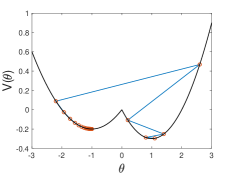
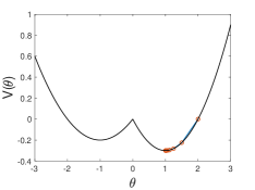
(1) Reweighting	(2) Resampling

Figure 1: Comparison of reweighting and resampling with $a_{1}/a_{2}=0.4/0.6$ and $f_{1}/f_{2}=0.9/0.1$ at the learning rate $\eta=0.5$. The resampling strategy here is to randomly select the sub-population $i$ with the probability $a_{i}$ with replacement in each iteration. (1) For reweighting, the trajectory starting from $\theta_{0}=1.1$ can end up at $\theta=-1$ after a few iterations, but $\theta=-1$ is not the global minimizer. (2) For resampling, the trajectory starting from $\theta_{0}=2.0$ stays close to the desired minimizer $\theta=1$. Hence resampling is more reliable than reweighting. We include more comparisons with various learning rates in Appendix D to show that resampling is stable for a wider range of $\eta$.

The expectations of the stochastic gradient are the same for both methods. It is the difference in the second moment that explains why trajectories near the two minima exhibit different behaviors. Our explanation is based on the stability analysis framework used in (Wu et al., 2018). By definition, a stationary point $\theta^{*}$ is stochastically stable if there exists a uniform constant $0<C\leq 1$ such that $\mathbb{E}[\lVert\theta_{k}-\theta^{*}\rVert^{2}]\leq C\lVert\theta_{0}-\theta^{*}\rVert^{2}$, where $\theta_{k}$ is the $k$-th iterate of SGD. The stability conditions for resampling and reweighting are stated in the following two lemmas, in which we use $\eta$ to denote the learning rate.

Lemma 1.

For resampling, the conditions for the SGD to be stochastically stable around $\theta=-1$ and $\theta=1$ are respectively

$$(1-\eta a_{1})^{2}+\eta^{2}a_{1}a_{2}\leq 1,\quad(1-\eta a_{2})^{2}+\eta^{2}a_{1}a_{2}\leq 1.$$

Lemma 2.

For reweighting, the condition for the SGD to be stochastically stable around $\theta=-1$ and $\theta=1$ are respectively

$$(1-\eta a_{1})^{2}+\eta^{2}f_{1}f_{2}\left(\frac{a_{1}}{f_{1}}\right)^{2}\leq 1,\quad(1-\eta a_{2})^{2}+\eta^{2}f_{1}f_{2}\left(\frac{a_{2}}{f_{2}}\right)^{2}\leq 1.$$

Note that the stability conditions for resampling are independent of the sampling proportions $(f_{1},f_{2})$, while the ones for reweighting clearly depend on $(f_{1},f_{2})$. We defer the detailed computations to Appendix A.

Lemma 2 shows that reweighting can incur a more stringent stability criterion. Let us consider the case $a_{1}=\frac{1}{2}-{\epsilon},a_{2}=\frac{1}{2}+{\epsilon}$ with a small constant ${\epsilon}>0$ and $f_{2}/f_{1}\ll 1$. For reweighting, the global minimum $\theta=1$ is stochastically stable only if $\eta(1+f_{1}/f_{2})\leq 4+O({\epsilon})$. This condition becomes rather stringent in terms of the learning rate $\eta$ since $f_{1}/f_{2}\gg 1$. On the other hand, the local minimizer $\theta=-1$ is stable if $\eta(1+f_{2}/f_{1})\leq 4+O({\epsilon})$, which could be satisfied for a broader range of $\eta$ because $f_{2}/f_{1}\ll 1$. In other words, for a fixed learning rate $\eta$, when the ratio $f_{2}/f_{1}$ between the sampling proportions is sufficiently small, the desired minimizer $\theta=1$ is no longer statistically stable with respect to SGD.

4 SDE analysis

The stability analysis can only be carried for a learning rate $\eta$ of a finite size. However, even for a small learning rate $\eta$, one can show that the reweighting method is still unreliable from a different perspective. This section applies stochastic differential equation analysis to demonstrate it.

Let us again use a simple example to illustrate the main idea. Consider the following two loss functions,

$$V_{1}(\theta)=\begin{cases}|\theta+1|-1,&\theta\leq 0\\ {\epsilon}\theta,&\theta>0\end{cases},\quad V_{2}(\theta)=\begin{cases}-{\epsilon}\theta,&\theta\leq 0\\ |\theta-1|-1,&\theta>0\end{cases},$$

with $0<{\epsilon}\ll 1$. The population loss function is $V(\theta)=a_{1}V_{1}(\theta)+a_{2}V_{2}(\theta)$ with local minimizers $\theta=-1$ and $\theta=1$. Note that the $O({\epsilon})$ terms are necessary. Without it, if the SGD starts in $(-\infty,0)$, all iterates will stay in this region because there is no drift from $V_{2}(\theta)$. Similarly, if the SGD starts in $(0,\infty)$, no iterates will move to $(-\infty,0)$. That means the result of SGD only depends on the initialization when $O({\epsilon})$ term is absent.

In Figure 2, we present numerical simulations of the resampling and reweighting methods for the designed loss function $V(\theta)$. If $a_{2}>a_{1}$, then the global minimizer of $V(\theta)$ is $\theta=1$ (see the Figure 2(1)). Consider a setup with population proportions $a_{1}/a_{2}=0.4/0.6$ along sampling proportions $f_{1}/f_{2}=0.9/0.1$, which are quite different. Figures 2(2) and (3) show the dynamics under the reweighting and resampling methods, respectively. The plots show that, while the trajectory for resampling is stable across time, the trajectory for reweighting quickly escapes to the (non-global) local minimizer $\theta=-1$ even when it starts near the global minimizer $\theta=1$.

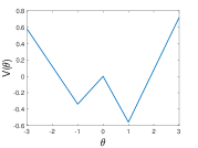
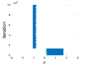
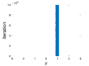
(1) Loss function $V(\theta)$	(2) Reweighting	(3) Resampling

Figure 2: Comparison of reweighting and resampling with learning rate $\eta=0.12$. We set $a_{1}/a_{2}=0.4/0.6$, $f_{1}/f_{2}=0.9/0.1$ and $\epsilon=0.1$. Both experiments start at $\theta_{0}=0.9$. The resampling strategy here is to randomly select the sub-population $i$ with the probability $a_{i}$ with replacement in each iteration. In (2) where reweighting is used, the trajectory skips to the local minimizer $\theta=-1$ later. In (3) where resampling is used, it stabilizes at the global minimizer $\theta=1$ all the time. We include more comparisons with various learning rates in Appendix D to show that resampling is more reliable for a wider range of $\eta$.

When the learning rate is sufficiently small, one can approximate the SGD by an SDE. Such a SDE approximation, first introduced in (Li et al., 2017), involves a data-dependent covariance coefficient for the diffusion term and is justified in the weak sense with an error of order $O(\sqrt{\eta})$. More specifically, the dynamics can be approximated by

$$d\Theta=-\nabla V(\Theta)dt+\sqrt{\eta}\Sigma(\Theta)^{1/2}dB,$$ (7)

where $\Theta(t=k\eta)\approx\theta_{k}$ for the step $k$ parameter $\theta_{k}$, $\eta$ is the learning rate, and $\Sigma(\Theta)$ is the covariance of the stochastic gradient at location $\Theta$. In the SDE theory, the drift term $\nabla V(\cdot)$ is usually assumed to be Lipschitz. However, in machine learning (for example neural network training with non-smooth activation functions), it is common to encounter non-Lipschitz gradients of loss functions (as in the example presented in Section 3). To fill this gap, we provide in Appendix C a justification of SDE approximation for the drift with jump discontinuities, based on the proof presented in (Müller-Gronbach et al., 2020).

In this piece-wise linear loss example, SGD can be approximated by a Langevin dynamics with a piecewise constant mobility. In particular when the dynamics reaches equilibrium, the stationary distribution of the stochastic process is approximated by a Gibbs distribution, which gives the probability densities at the stationary points. Let us denote $p_{s}(\theta)$ and $p_{w}(\theta)$ as the stationary distribution over $\theta$ under resampling and reweighting, respectively. Following lemmas quantitatively summarize the results.

Lemma 3.

When $a_{2}>a_{1}$, $V(1)<V(-1)$. The stationary distribution for resampling satisfies the relationship

$$\frac{p_{s}(1)}{p_{s}(-1)}=\exp\left(-\frac{2}{a_{1}a_{2}\eta}(V(1)-V(-1))\right)+O\left({\epsilon}\right)>1.$$

Lemma 4.

With $a_{2}>a_{1}$, $V(1)<V(-1)<0$. Under the condition $\frac{f_{2}}{f_{1}}\leq\frac{a_{2}}{a_{1}}\sqrt{\frac{V(-1)}{V(1)}}$ for the sampling proportions, the stationary distribution for reweighting satisfies the relationship

$$\frac{p_{w}(1)}{p_{w}(-1)}=\frac{a_{1}^{2}/f_{1}^{2}}{a_{2}^{2}/f_{2}^{2}}\exp\left(-\frac{2f_{2}/f_{1}}{a_{2}^{2}\eta}V(1)+\frac{2f_{1}/f_{2}}{a_{1}^{2}\eta}V(-1)\right)+O({\epsilon})<1.$$

The proofs of the above two lemmas can be found in Appendix B. Lemma 3 shows that for resampling it is always more likely to find $\theta$ at the global minimizer $1$ than at the local minimizer $-1$. Lemma 4 states that for reweighting it is more likely to find $\theta$ at the local minimizer $-1$ when $\frac{f_{2}}{f_{1}}\leq\frac{a_{2}}{a_{1}}\sqrt{\frac{V(-1)}{V(1)}}$. Together, they explain the phenomenon shown in Figure 2.

To better understand the condition in Lemma 4, let us consider the case $a_{1}=\frac{1}{2}-{\epsilon},a_{2}=\frac{1}{2}+{\epsilon}$ with a small constant ${\epsilon}>0$. Under this setup, $V(-1)/V(1)\approx 1$. Whenever the ratio of the sampling proportions $f_{2}/f_{1}$ is significantly less than the ratio of the population proportions $a_{2}/a_{1}\approx 1$, reweighting will lead to the undesired behavior. The smaller the ratio $f_{2}/f_{1}$ is, the less likely the global minimizer will be visited.

Piecewise Convex results.

The reason for constructing the above piecewise linear loss function is to obtain an approximately explicitly solvable SDE with a constant coefficient for the noise. One can further extend the results in 1D for piecewise strictly convex function with two local minima (See Lemmas 8 and 9 in Appendix B.3). Here we present the most general results in 1D, that is, piecewise strictly convex function with finite number of local minima. One may consider the population loss function $V(\theta)=\sum_{i=1}^{k}a_{i}V_{i}(\theta)$ with $V_{i}(\theta)=h_{i}(\theta)$ for $\theta_{i-1}<\theta\leq\theta_{i}$ and $V_{i}(\theta)=O({\epsilon})$ otherwise, where $h_{i}(\theta)$ are strictly convex functions and continuously differentiable, $O({\epsilon})$ term is sufficiently small and smooth. Here $\{\theta_{i}\}_{i=1}^{k-1}$ are $k-1$ disjoint points, and $\theta_{0}=-\infty,\theta_{k}=\infty$. We assume that $V(\theta)$ has $k$ local minimizers $\theta_{i}^{*}$ for $\theta_{i}^{*}\in(\theta_{i-1},\theta_{i})$. We present the following two lemmas with suitable assumptions (See Appendix B.3 for details of assumptions and the proof).

Lemma 5.

The stationary distribution for resampling at any two local minizers $\theta_{p}^{*},\theta_{q}^{*}$ with $p>q$ satisfies the relationship

$$\frac{p_{s}(\theta_{p}^{*})}{p_{s}(\theta_{q}^{*})}=\exp\left[\frac{2}{\eta}\int_{\theta_{p}^{*}}^{\theta_{p}}\frac{1}{h_{p}^{\prime}(\theta)}d\theta\,\left(\frac{1}{1-a_{p}}-\frac{1}{1-a_{q}}\right)\right]+O({\epsilon})=\left\{\begin{aligned} &>1,\quad\text{if }a_{p}>a_{q};\\ &<1,\quad\text{if }a_{p}<a_{q},\end{aligned}\right.$$

Lemma 6.

The stationary distribution for reweighting at any two local minizers $\theta_{p}^{*},\theta_{q}^{*}$ with $p>q$ satisfies the relationship

$$\frac{p_{w}(\theta_{p}^{*})}{p_{w}(\theta_{q}^{*})}=\exp\left[\frac{2}{\eta}\int_{\theta_{p}^{*}}^{\theta_{p}}\frac{1}{h_{p}^{\prime}(\theta)}d\theta\,\left(\frac{f_{p}}{a_{p}(1-f_{p})}-\frac{f_{q}}{a_{q}(1-f_{q})}\right)\right]+O({\epsilon}).$$

We first note that $\int_{\theta_{p}^{*}}^{\theta_{p}}\frac{1}{h^{\prime}_{p}(\theta)}d\theta>0$ due to the strictly convexity of $h_{p}$. Therefore, one can see from Lemma 5 that for resampling, the stationary solution always has the highest probability at the global minimizer. On the other hand, for the stationary solution of reweighting in Lemma 6, let us consider the case when $a_{p}>a_{q}$. In this case, $V(\theta_{p}^{*})<V(\theta_{q}^{*})$, therefore, one expects the above ratio larger than $1$, which implies that $\frac{f_{p}}{a_{p}(1-f_{p})}-\frac{f_{q}}{a_{q}(1-f_{q})}>0$. Note that if $f_{p}=a_{p},f_{q}=a_{q}$, then this term is always larger than $0$, but when $f_{p},f_{q}$ are significantly different from $a_{p},a_{q}$ in the sense that $f_{p}<f_{q}$ and $f_{p}<a_{p},f_{q}>a_{q}$, then $\frac{f_{p}}{a_{p}(1-f_{p})}-\frac{f_{q}}{a_{q}(1-f_{q})}<0$, which will lead to $\frac{p_{s}(\theta_{p}^{*})}{p_{s}(\theta_{q}^{*})}<1$, i.e., higher probability of converging to $\theta_{q}^{*}$, which is not desirable. To sum up, Lemma 6 shows that for reweighting, the stationary solution will not have the highest probability at the global minimizer if the empirical proportion is significantly different from the population proportion.

Multi-dimensional results.

It is in fact not clear how to extend Lemmas 5 and 6 to multi-dimension. As far as we know, it is still an open problem how the stochastic process behaves when the covariance matrix of (7) depends on $\Theta$ in high dimensions. Instead, we focus on the case where the covariance matrix is piecewise constant. We divide the whole space into a finite number of disjoint convex regions $\mathbb{R}^{d}=\cup_{i=1}^{k}\Omega_{i}$. The loss function $V(\bm{\theta})=\sum_{i=1}^{k}a_{i}V_{i}(\bm{\theta})$ with $V_{i}(\bm{\theta})=\kappa_{i}\left\lVert\bm{\theta}-\bm{\theta}_{i}^{*}\right\rVert_{1}-\beta_{i}$ for $\bm{\theta}\in\Omega_{i}$ and $V_{i}(\bm{\theta})=O({\epsilon})$ otherwise, where $\left\lVert\bm{\theta}\right\rVert_{1}=\sum_{j=1}^{d}|\theta_{j}|$. The loss function has $k$ local minimizers $\bm{\theta}_{i}^{*}\in\Omega_{i}$. The following Lemma summarizes the results for the multi-dimensional case.

Lemma 7.

The stationary distribution for resampling and reweighting at any two local minimizers $\bm{\theta}_{p}^{*},\bm{\theta}_{q}^{*}$ satisfies the relationship

$$\frac{p_{s}(\bm{\theta}_{p}^{*})}{p_{s}(\bm{\theta}_{q}^{*})}=\exp\left[\frac{2}{\eta}\left(\frac{\beta_{p}}{(1-a_{p})\kappa_{p}^{2}}-\frac{\beta_{q}}{(1-a_{q})\kappa_{q}^{2}}\right)\right]+O({\epsilon}),$$

$$\frac{p_{w}(\bm{\theta}_{p}^{*})}{p_{w}(\bm{\theta}_{q}^{*})}=\exp\left[\frac{2}{\eta}\left(\frac{f_{p}\beta_{p}}{a_{p}(1-f_{p})\kappa_{p}^{2}}-\frac{f_{q}\beta_{q}}{a_{q}(1-f_{q})\kappa_{q}^{2}}\right)\right]+O({\epsilon}),$$

respectively.

The proof of the above lemma together with the interpretation can be found in Appendix B.4.

5 Experiments

This section examines the empirical performance of resampling and reweighting for problems from classification, regression, and reinforcement learning. As mentioned in the previous sections, the noise of stochastic gradient algorithms makes optimal learning rate selections much more restrictive for reweighting, when the data sampling is highly biased. In order to achieve good learning efficiency and reasonable performance in a neural network training, adaptive stochastic gradient methods such as Adam (Kingma & Ba, 2014) are applied in the first two experiments. We observe that resampling consistently outperforms reweighting with various sampling ratios when combined with these adaptive learning methods.

Classification.

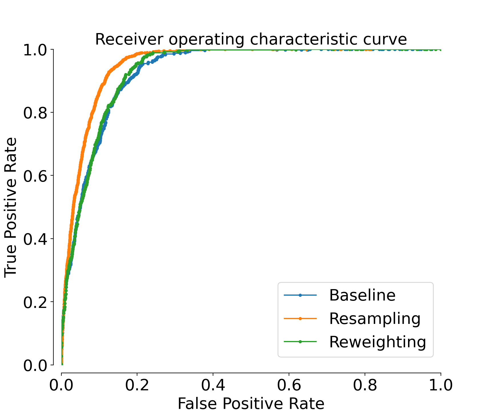
Figure 3: The ROC curve comparisons show that the resampling has the largest area under the curve.

This experiment uses the Bank Marketing data set from (Moro et al., 2014) to predict if a client will subscribe a term deposit. After preprocessing, the provided data distribution over the variable “y” that indicates the subscription, is highly skewed: the ratio of “yes” and “no” is $f_{1}/f_{2}=4640/36548\approx 1/7.88$. We assume that the underlying population distribution is $a_{1}/a_{2}=1$. We setup a 3-layer neural network with the binary cross-entropy loss function and train with the default Adam optimizer. The training and testing data set is obtained using train_test_split provided in sklearn. The training takes 5 epochs with the batch-size equal to 100. The performance is compared among the baseline (i.e. trained without using either resampling or reweighting), resampling (oversample the minority group uses the sample with replacement), and reweighting. We run the experiments 10 times for each case, and then compute and plot results by averaging.

	Baseline	Resampling	Reweighting
training loss	0.3221	0.2602	0.2831
roc_auc_score	0.9277	0.9516	0.9312

Table 1: The loss takes the binary cross-entropy with a 3-layer neural network. We see that in average of 10 trials, the resampling method (oversampling) achieves the lowest training loss and highest ROC-AUC score over testing data among all tested cases.

To estimate the performance, rather than using the classification accuracy that can be misleading for biased data, we use the metric that computes the area under the receiver operating characteristic curve (ROC-AUC) from the prediction scores. The ROC curves plots the true positive rate on the $y$-axis versus the false positive rate on the $x$-axis. As a result, a larger area under the curve indicates a better performance of a classifier. From both Table 1 and Figure 3, we see that the oversampling has the best performance compared to others. We choose oversampling rather than undersampling for the resampling method, because if we naively down sample the majority group, we throw away many information that could be useful for the prediction.

Nonlinear Regression.

This experiment uses the California Housing Prices data set to predict the median house values. The target median house values, ranging from $15$k to $500$k, are distributed quite non-uniformly. We select subgroups with median house values $>400$k ($1726$ in total) and $<200$k ($11767$ in total) and combine them to make our dataset. In the pre-processing step, we drop the “ocean proximity” feature and randomly set $30\%$ of the data to be the test data. The remaining training data set with $8$ features is fed into a 3-layer neural network. The population proportion of two subgroups is assumed to be $a_{1}/a_{2}\approx 1$, while resampling and reweighting are tested with various sampling ratios $f_{1}/f_{2}$ near $11767/1726$. Their performance of is compared also with the baseline. In each test, the mean squared error (MSE) is chosen as the loss function and Adam is used as the optimizer in the model. The batch-size is $32$ and the number of epochs is $400$ for each case. As shown in Table 2, resampling significantly outperforms reweighting for all sampling ratios in terms of a lower averaged MSE, and its good stability is reflected in its lowest standard deviation for multiple runs.

MSE	Baseline	RS	RW ($f_{1}/f_{2}=7$)	RW ($f_{1}/f_{2}=9$)	RW ($f_{1}/f_{2}=12$)
mean	1.0386e+05	7.9679e+04	9.3567e+04	9.0436e+04	9.1949e+04
std	8.0371e+03	1.8620e+03	3.8044e+03	2.4692e+03	3.0341e+03

Table 2: Mean squared errors (MSE) for nonlinear regression problems. RS stands for resampling and RW for reweighting. The weights used in reweighting are $\frac{a_{1}}{f_{1}}$ and $\frac{a_{2}}{f_{2}}$, respectively. For each case, we run experiments for 10 times and compute the corresponding mean and standard deviation. Resampling (oversampling the minor group) achieves the lowest mean and standard deviation of MSE among all tested cases.

Off-policy prediction.

In the off-policy prediction problem in reinforcement learning, the objective is to find the value function of policy $\pi$ using the trajectory $\{(a_{t},s_{t},s_{t+1})\}_{t=1}^{T}$ generated by a behavior policy $\mu$. To achieve this, the standard approach is to update the value function based on the behavior policy’s temporal difference (TD) error $\delta(s_{t})=R(s_{t})+\gamma V(s_{t+1})-V(s_{t})$ with an importance weight $\mathbb{E}_{\pi}[\delta|s_{t}=s]=\sum_{a\in\mathbb{A}}\frac{\pi(a|s)}{\mu(a|s)}\mathbb{E}[\delta|s_{t}=s,a_{t}=a]\mu(a|s)$, where the summation is taken over the action space $\mathbb{A}$. The resulting reweighting TD learning for policy $\pi$ is

$$V_{t+1}(s_{t})=V_{t}(s_{t})+\eta\frac{\pi(a_{t}|s_{t})}{\mu(a_{t}|s_{t})}(R(s_{t})+\gamma V_{t}(s_{t+1})-V_{t}(s_{t})),$$

where $\eta$ is the learning rate. This update rule is an example of reweighting. On the other hand, the expected TD error can also be written in the resampling form, $\mathbb{E}_{\pi}[\delta|s_{t}=s]=\sum_{a\in\mathbb{A}}\mathbb{E}[\delta|s_{t}=s,a_{t}=a]\pi(a|s)=\sum_{a\in\mathbb{A}}\sum_{j=1}^{\pi(a|s)N}\mathbb{E}[\delta^{j}|s_{t}=s,a_{t}=a]$, where $N$ is the total number of samples for $s_{t}=s$. This results to a resampling TD learning algorithm: at step $t$,

$$V_{t+1}(s_{t})=V_{t}(s_{t})+\eta(R(s_{k})+\gamma V_{t}(s_{k+1})-V_{t}(s_{k})),$$

where $(a_{k},s_{k},s_{k+1})$ is randomly chosen from the data set $\{(a_{j},s_{j},s_{j+1})\}_{s_{j}=s_{t}}$ with probability $\pi(a_{k}|s_{t})$.

Consider a simple example with discrete state space $\mathbb{S}=\{i\}_{i=0}^{n-1}$, action space $\mathbb{A}=\{\pm 1\}$, discount factor $\gamma=0.9$ and transition dynamics $s_{t+1}=\text{mod}(s_{t}+a_{t},n)$, where the operator $\mod(m,n)$ gives the remainder of $m$ divided by $n$. Figure 4 shows the results of the off-policy TD learning by these two approaches, with the choice of $n=32$ and $r(s)=1+\sin(2\pi s/n)$ and learning rate $\eta=0.1$. The target policy is $\pi(a_{i}|s)=\frac{1}{2}$ while the behavior policy is $\mu(a_{i}|s)=\frac{1}{2}+ca_{i}$. The difference between the two policies becomes larger as the constant $c\in[0,1/2]$ increases. From the previous analysis, if one group has much fewer samples as it should have, then the minimizer of the reweighting method is highly affected by the sampling bias. This is verified in the plots: as $c$ becomes larger, the performance of reweighting deteriorates, while resampling is rather stable and almost experiences no difference with the on-policy prediction in this example.

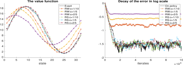
Figure 4: The left plot shows the approximate value function obtained by the two methods. The right plot is the evolution of the relative error $\log(\frac{{e}_{t}}{{e}_{0}})$, where the absolute error ${e}_{t}=\lVert V_{t}(s)-V^{\pi}(s)\rVert^{2}_{2}.$ RW and RS in the upright corner represent reweighting and resampling, respectively. $c$ determines the behavior policy $\mu(a_{i}|s)=\frac{1}{2}+ca_{i}$. The value function is trained on a trajectory with length $10^{5}$ generated by the behavior policy. The value function obtained from resampling is fairly close to the exact value function, while the results of reweighting gets worse as the behavior policy gets further from the target policy.

6 Discussions

This paper examines the different behaviors of reweighting and resampling for training on biasedly sampled data with the stochastic gradient descent. From both the dynamical stability and stochastic asymptotics viewpoints, we explain why resampling is numerically more stable and robust than reweighting. Based on this theoretical understanding, we advocate for considering data, model, and optimization as an integrated system, while addressing the bias.

An immediate direction for future work is to apply the analysis to more sophisticated stochastic training algorithms and understand their impact on resampling and reweighting. Another direction is to extend our analysis to unsupervised learning problems. For example, in the principal component analysis one computes the dominant eigenvectors of the covariance matrix of a data set. When the data set consists of multiple subgroups sampled with biases and a stochastic algorithm is applied to compute the eigenvectors, then an interesting question is how resampling or reweighting would affect the result.

Appendix A Proofs in section 3

A.1 Proof of Lemma 1

Proof.

In resampling, near $\theta=-1$ the gradient is $\theta+1$ with probability $a_{1}$ and $0$ with probability $a_{2}$. Let us denote the random gradient at each step by $W(\theta+1)$, where $W$ is a Bernoulli random variable with mean $\mathbb{E}(W)=a_{1}$ and variance $\mathbb{V}(W)=a_{1}a_{2}$. At the learning rate $\eta$, the iteration can be written as

$$(\theta_{k+1}+1)=(1-\eta W)(\theta_{k}+1).$$

The first and second moments of the iterates are

$$\mathbb{E}[\theta_{k}+1] =(1-\eta a_{1})^{k}(\theta_{0}+1),$$ (8)

$$\mathbb{E}[(\theta_{k}+1)^{2}] =((1-\eta a_{1})^{2}+\eta^{2}a_{1}a_{2})^{k}(\theta_{0}+1)^{2}.$$

According to the definition of the stochastic stability, SGD is stable around $\theta=-1$ if the multiplicative factor of the second equation is bounded by $1$, i.e.

$$(1-\eta a_{1})^{2}+\eta^{2}a_{1}a_{2}\leq 1.$$ (9)

Consider now the stability around $\theta=1$, the iteration can be written as

$$(\theta_{k+1}-1)=(1-\eta W)(\theta_{k}-1),$$

where $W$ is again a Bernoulli random variable with $\mathbb{E}(W)=a_{2}$ and $\mathbb{V}(W)=a_{1}a_{2}$. The same computation shows that the second moment follows

$$\mathbb{E}[(\theta_{k}-1)^{2}]=((1-\eta a_{2})^{2}+\eta^{2}a_{1}a_{2})^{k}(\theta_{0}-1)^{2}.$$

Therefore, the condition for the SGD to be stable around $\theta=1$ is

$$(1-\eta a_{2})^{2}+\eta^{2}a_{1}a_{2}\leq 1.$$ (10)

∎

A.2 Proof of Lemma 2

Proof.

In reweighting, near $\theta=-1$ the gradient is $\frac{a_{1}}{f_{1}}(\theta+1)$ with probability $f_{1}$ and $0$ with probability $f_{2}$. Let us denote the random gradient at each step by $W(\theta+1)$, where $W$ is a Bernoulli random variable with $\mathbb{E}(W)=a_{1}$ and $\mathbb{V}(W)=f_{1}f_{2}\left(\frac{a_{1}}{f_{1}}\right)^{2}$. At the learning rate $\eta$, the iteration can be written as

$$(\theta_{k+1}+1)\leftarrow(1-\eta W)(\theta_{k}+1).$$

Hence the second moments of the iterates are given by

$$\mathbb{E}[(\theta_{k}+1)^{2}]=((1-\eta a_{1})^{2}+\eta^{2}f_{1}f_{2}(a_{1}/f_{1})^{2})^{k}(\theta_{0}+1)^{2}.$$

Therefore, the condition for the SGD to be stable around $\theta=-1$ is

$$(1-\eta a_{1})^{2}+\eta^{2}f_{1}f_{2}\left(\frac{a_{1}}{f_{1}}\right)^{2}\leq 1.$$

Consider now the stability around $\theta=1$, the gradient is $0$ with probability $f_{1}$ and $\frac{a_{2}}{f_{2}}(\theta-1)$ with probability $f_{2}$. An analysis similar to the case $\theta=-1$ shows that the condition for the SGD to be stable around $\theta=1$ is

$$(1-\eta a_{2})^{2}+\eta^{2}f_{1}f_{2}\left(\frac{a_{2}}{f_{2}}\right)^{2}\leq 1.$$

∎

Appendix B Proofs in section 4

B.1 Proof of Lemma 3

Proof.

In resampling, with probability $a_{1}$ the gradients over the four intervals $(-\infty,-1)$, $(-1,0)$, $(0,1)$, and $(1,\infty)$ are $-1$, $1$, ${\epsilon}$, and ${\epsilon}$. With probability $a_{2}$, they are $-{\epsilon}$, $-{\epsilon}$, $-1$, and $1$ across these four intervals. The variances of the gradients are $a_{1}a_{2}(1-{\epsilon})^{2}$, $a_{1}a_{2}(1+{\epsilon})^{2}$, $a_{1}a_{2}(1+{\epsilon})^{2}$, $a_{1}a_{2}(1-{\epsilon})^{2}$, respectively, across the same intervals.

Since ${\epsilon}\ll 1$, the variance can be written as $a_{1}a_{2}+O({\epsilon})$ across all intervals. Then the SGD dynamics with learning rate $\eta$ can be approximated by

$$\theta_{k+1}\leftarrow\theta_{k}-\eta\left(V^{\prime}(\theta_{k})+\sqrt{a_{1}a_{2}+O({\epsilon})}W\right),$$

where $W\sim\mathcal{N}(0,1)$ is a normal random variable. When $\eta$ is small, one can approximate the dynamics by a stochastic differential equation of form

$$d\Theta=-V^{\prime}(\Theta)dt+\sqrt{\eta}\sqrt{a_{1}a_{2}+O({\epsilon})}dB$$

by identifying $\theta_{k}\approx\Theta(t=k\eta)$ (see Appendix C for details). The stationary distribution of this stochastic process is

$$p_{s}(\theta)=\frac{1}{Z}\exp\left(-\frac{2}{(a_{1}a_{2}+O({\epsilon}))\eta}V(\theta)\right),$$

where $Z$ is a normalization constant. Plugging in $\theta=-1,1$ results in

$$\frac{p_{s}(1)}{p_{s}(-1)}= \exp\left(-\frac{2}{(a_{1}a_{2}+O({\epsilon}))\eta}\left(V(1)-V(-1)\right)\right)=\exp\left(-\frac{2}{a_{1}a_{2}\eta}(V(1)-V(-1))+O({\epsilon})\right)$$

$$= \exp\left(-\frac{2}{a_{1}a_{2}\eta}(V(1)-V(-1))\right)+O({\epsilon}).$$

Under the assumption that ${\epsilon}\ll 1$, the last term is negligible. When $a_{2}>a_{1}$, $V(\theta)$ is minimized at $\theta=1$, which implies $-(V(1)-V(-1))>0$. Hence, this ratio is larger than 1. ∎

B.2 Proof of Lemma 4

Proof.

In reweighting, with probability $f_{1}$ the gradients are $-\frac{a_{1}}{f_{1}}$, $\frac{a_{1}}{f_{1}}$, $\frac{a_{1}}{f_{1}}{\epsilon}$, and $\frac{a_{1}}{f_{1}}{\epsilon}$ over the four intervals $(-\infty,-1)$, $(-1,0)$, $(0,1)$, and $(1,\infty)$, respectively. With probability $f_{2}$, they are $-\frac{a_{2}}{f_{2}}{\epsilon}$, $-\frac{a_{2}}{f_{2}}{\epsilon}$, $-\frac{a_{2}}{f_{2}}$, and $\frac{a_{2}}{f_{2}}$. The variances of the gradients are $f_{1}f_{2}(\frac{a_{1}}{f_{1}}-\frac{a_{2}}{f_{2}}{\epsilon})^{2}$, $f_{1}f_{2}(\frac{a_{1}}{f_{1}}+\frac{a_{2}}{f_{2}}{\epsilon})^{2}$, $f_{1}f_{2}(\frac{a_{1}}{f_{1}}{\epsilon}+\frac{a_{2}}{f_{2}})^{2}$, and $f_{1}f_{2}(\frac{a_{1}}{f_{1}}{\epsilon}-\frac{a_{2}}{f_{2}})^{2}$, respectively, across the same intervals.

Since ${\epsilon}\ll 1$, the variance can be written as $f_{1}f_{2}\frac{a_{1}^{2}}{f_{1}^{2}}+O({\epsilon})$ for $\theta<0$ and $f_{1}f_{2}\frac{a_{2}^{2}}{f_{2}^{2}}+O({\epsilon})$ for $\theta>0$.

With $\theta_{k}\approx\Theta(k\eta)$, the approximate SDE for $\theta<0$ is given by

$$d\Theta=-V^{\prime}(\Theta)dt+\sqrt{\eta}\sqrt{f_{1}f_{2}\frac{a_{1}^{2}}{f_{1}^{2}}+O({\epsilon})}dB$$

while the one for $\theta>0$ is

$$d\Theta=-V^{\prime}(\Theta)dt+\sqrt{\eta}\sqrt{f_{1}f_{2}\frac{a_{2}^{2}}{f_{2}^{2}}+O({\epsilon})}dB$$

(see Appendix C for the SDE derivations). The stationary distributions for $\theta<0$ and $\theta>0$ are, respectively,

$$\frac{1}{Z_{1}}\exp\left(-\frac{2}{\left(f_{1}f_{2}\frac{a_{1}^{2}}{f_{1}^{2}}+O({\epsilon})\right)\eta}V(\theta)\right),\quad\frac{1}{Z_{2}}\exp\left(-\frac{2}{\left(f_{1}f_{2}\frac{a_{2}^{2}}{f_{2}^{2}}+O({\epsilon})\right)\eta}V(\theta)\right).$$

Plugging in $\theta=-1,1$ results in

$$\frac{p_{w}(1)}{p_{w}(-1)}= \frac{Z_{1}}{Z_{2}}\exp\left(-\frac{2}{\left(f_{1}f_{2}\frac{a_{2}^{2}}{f_{2}^{2}}+O({\epsilon})\right)\eta}V(1)+\frac{2}{\left(f_{1}f_{2}\frac{a_{1}^{2}}{f_{1}^{2}}+O({\epsilon})\right)\eta}V(-1)\right)$$ (11)

$$= \frac{Z_{1}}{Z_{2}}\exp\left(-\frac{2f_{2}/f_{1}}{a_{2}^{2}\eta}V(1)+\frac{2f_{1}/f_{2}}{a_{1}^{2}\eta}V(-1)+O({\epsilon})\right).$$

The next step is to figure out the relationship between $Z_{1}$ and $Z_{2}$. Consider an SDE with non-smooth diffusion $d\Theta=-V^{\prime}(\Theta)dt+\sigma dB$. The Kolmogorov equation for the stationary distribution is

$$0=p_{t}=\left(V^{\prime}(\theta)p+\left(\frac{\sigma^{2}}{2}p\right)_{\theta}\right)_{\theta}.$$ (12)

This suggests that $\sigma^{2}p$ is continuous at the discontinuity $\theta=0$. In our setting, since $V(0)=0$, this simplifies to

$$\left(f_{1}f_{2}\frac{a_{1}^{2}}{f_{1}^{2}}+O({\epsilon})\right)\eta\cdot\frac{1}{Z_{1}}=\left(f_{1}f_{2}\frac{a_{2}^{2}}{f_{2}^{2}}+O({\epsilon})\right)\eta\cdot\frac{1}{Z_{2}}.$$

This simplifies to

$$\frac{Z_{1}}{Z_{2}}=\frac{f_{1}f_{2}\frac{a_{1}^{2}}{f_{1}^{2}}+O({\epsilon})}{f_{1}f_{2}\frac{a_{2}^{2}}{f_{2}^{2}}+O({\epsilon})}=\frac{a_{1}^{2}/f_{1}^{2}}{a_{2}^{2}/f_{2}^{2}}+O({\epsilon}).$$

Inserting this into (11) results in

$$\frac{p_{w}(1)}{p_{w}(-1)}= \left(\frac{a_{1}^{2}/f_{1}^{2}}{a_{2}^{2}/f_{2}^{2}}+O({\epsilon})\right)\exp\left(-\frac{2f_{2}/f_{1}}{a_{2}^{2}\eta}V(1)+\frac{2f_{1}/f_{2}}{a_{1}^{2}\eta}V(-1)+O({\epsilon})\right)$$

$$= \frac{a_{1}^{2}/f_{1}^{2}}{a_{2}^{2}/f_{2}^{2}}\exp\left(-\frac{2f_{2}/f_{1}}{a_{2}^{2}\eta}V(1)+\frac{2f_{1}/f_{2}}{a_{1}^{2}\eta}V(-1)\right)+O({\epsilon}).$$

By the assumption $\frac{f_{2}}{f_{1}}\leq\frac{a_{2}}{a_{1}}\sqrt{\frac{V(-1)}{V(1)}}$ and $V(1)<V(-1)<0$, one has $\left(\frac{a_{1}}{a_{2}}\right)^{2}\left(\frac{f_{2}}{f_{1}}\right)^{2}\leq\frac{V(-1)}{V(1)}<1$ and $-\frac{f_{2}/f_{1}}{a_{2}^{2}}V(1)\leq-\frac{f_{1}/f_{2}}{a_{1}^{2}}V(-1)$. Hence the above ratio is less than $1$. ∎

B.3 Extended results for $1$-dimension

Let us consider the population loss function $V(\theta)=a_{1}V_{1}(\theta)+a_{2}V_{2}(\theta)$ with,

$$V_{1}(\theta)=\begin{cases}h_{1}(\theta),&\theta\leq 0\\ {\epsilon}\theta,&\theta>0\end{cases},\quad V_{2}(\theta)=\begin{cases}-{\epsilon}\theta,&\theta\leq 0\\ h_{2}(\theta),&\theta>0\end{cases},$$

where $h_{1},h_{2}$ are strictly convex functions and continuously differentiable. We assume $V(\theta)$ has two local minimizers $\theta_{1}<0,\theta_{2}>0$ and the values are negative at local minima. Therefore, when $a_{2}>a_{1}$, $\theta_{2}$ should be the global minimizer. In addition, we assume that the geometries of $h_{1},h_{2}$ at two local minimizers are similar, i.e., $h_{1}(\theta_{1})=h_{2}(\theta_{2})$, $h_{1}^{\prime}(\theta_{1})=h_{2}^{\prime}(\theta_{2})$; if we set $g_{i}(\theta)$ to be the anti-derivative of $1/h^{\prime}_{i}(\theta)$, then $g_{1}(\theta_{1})=g_{2}(\theta_{2})$. Moreover, we assume that the two disjoint convex functions are smooth at the disjoint point, i.e., $h_{1}^{\prime}(0)=h_{2}^{\prime}(0)$ and $g_{1}(0)=g_{2}(0)$. The following two lemmas extend Lemmas 3 and 4 to piecewise strictly convex function based on the above assumptions.

Lemma 8.

When $a_{2}>a_{1}$, $V(\theta_{2})<V(\theta_{1})$. The stationary distribution for resampling satisfies the relationship

$$\frac{p_{s}(\theta_{2})}{p_{s}(\theta_{1})}=\exp\left(\frac{2}{\eta}\left(\frac{1}{a_{1}}-\frac{1}{a_{2}}\right)\int_{\theta_{1}}^{0}\frac{1}{h_{1}^{\prime}(\theta)}d\theta\right)+O({\epsilon})>1.$$

Proof.

In resampling, with probability $a_{1}$ the gradients in the two intervals $(-\infty,0),(0,\infty)$ are $h_{1}^{\prime}(\theta),{\epsilon}$ respectively; with probability $a_{2}$ the gradients are $-{\epsilon},h_{2}^{\prime}(\theta)$ respectively. Therefore, the expectation of the gradients $\mu(\theta)$ is $a_{1}h^{\prime}_{1}(\theta)+O({\epsilon})$ in $(-\infty,0)$ and $a_{2}h^{\prime}_{2}(\theta)+O({\epsilon})$ in $(0,\infty)$. The variance of the gradients $\sigma(\theta)$ is $a_{1}a_{2}h_{1}^{\prime}(\theta)^{2}+O({\epsilon})$ in $(-\infty,0)$ and $a_{1}a_{2}h^{\prime}_{2}(\theta)^{2}+O({\epsilon})$ in $(0,\infty)$. The p.d.f $p_{s}(t,\theta)$ satisfies

$$\partial_{t}p_{s}=\partial_{\theta}\left(\mu p_{s}+\frac{\eta}{2}{\partial_{\theta}(\sigma p_{s})}\right),$$

therefore, the stationary distribution $p_{s}(\theta)$ satisfies

$$\left(\mu+\frac{\eta}{2}\partial_{\theta}\sigma\right)p_{s}+\frac{\eta\sigma}{2}\partial_{\theta}p_{s}=0,\quad\text{or equivalently, }\quad\left(\frac{2\mu}{\eta\sigma}+\frac{\partial_{\theta}\sigma}{\sigma}\right)p_{s}+\partial_{\theta}p_{s}=0,$$

which implies $p_{s}(\theta)=\frac{1}{Z}e^{-F(\theta)}$ with normalization constant $Z=\int_{-\infty}^{\infty}e^{-F(\theta)}$, where

$$F(\theta)=\int_{-\infty}^{\theta}\frac{2\mu(\xi)}{\eta\sigma(\xi)}+\frac{\partial_{\xi}\sigma(\xi)}{\sigma(\xi)}d\xi=\left\{\begin{aligned} &F_{1}(\theta)-F_{1}(-\infty),\quad\theta\leq 0,\\ &F_{2}(\theta)-F_{2}(0)+F_{1}(0)-F_{1}(-\infty),\quad\theta>0.\end{aligned}\right.$$ (13)

By inserting $\mu,\sigma$ in different intervals, one has

$$\left\{\begin{aligned} &F_{1}(\theta)=\frac{2}{\eta a_{2}}\int\frac{1}{h_{1}^{\prime}}d\theta+\log(a_{1}a_{2}(h_{1}^{\prime})^{2})+O({\epsilon});\\ &F_{2}(\theta)=\frac{2}{\eta a_{1}}\int\frac{1}{h_{2}^{\prime}}d\theta+\log(a_{1}a_{2}(h_{2}^{\prime})^{2})+O({\epsilon}).\end{aligned}\right.$$

Hence, the ratio of the stationary probabiliy at two local minimizers $\theta_{1}<0,\theta_{2}>0$ is

$$\frac{p_{s}(\theta_{1})}{p_{s}(\theta_{2})}= \exp(-F(\theta_{1})+F(\theta_{2}))=\exp(-F_{1}(\theta_{1})+F_{2}(\theta_{2})+(F_{1}(0)-F_{2}(0)))$$

$$= \exp\left(-\frac{2}{\eta a_{2}}g_{1}(\theta_{1})+\frac{2}{\eta a_{1}}g_{2}(\theta_{2})+\log\left(\frac{h_{2}^{\prime}(\theta_{2})^{2}}{h_{1}^{\prime}(\theta_{1})^{2}}\right)\right)\cdot$$

$$\exp\left(\frac{2}{\eta a_{2}}g_{1}(0)-\frac{2}{\eta a_{1}}g_{2}(0)+\log\left(\frac{h_{1}^{\prime}(0)^{2}}{h_{2}^{\prime}(0)^{2}}\right)\right)+O({\epsilon}),$$

where $g_{i}(\theta)=\int\frac{1}{h_{i}^{\prime}}d\theta,i=1,2$. By the assumption that $g_{1}(\theta_{1})=g_{2}(\theta_{2})$ and $h^{\prime}_{1}(\theta_{1})=h_{2}^{\prime}(\theta_{2})$, $g_{1}(0)=g_{2}(0)$ and $h^{\prime}_{1}(0)=h_{2}^{\prime}(0)$ one has,

$$\frac{p_{s}(\theta_{1})}{p_{s}(\theta_{2})}=\exp\left(\frac{2}{\eta}(g_{1}(0)-g_{1}(\theta_{1}))\left(\frac{1}{a_{2}}-\frac{1}{a_{1}}\right)\right)+O({\epsilon}),$$

Since $a_{2}>a_{1}>0$, $\frac{1}{a_{2}}-\frac{1}{a_{1}}<0$. Because of the strictly convexity of $h_{1}$, $h_{1}^{\prime}(\theta)>0$ in $(\theta_{1},0)$, therefore, one has $g_{1}(0)-g_{1}(\theta_{1})=\int_{\theta_{1}}^{0}\frac{1}{h_{1}^{\prime}(\theta)}d\theta>0$. Therefore

$$\frac{p_{s}(\theta_{1})}{p_{s}(\theta_{2})}=\exp\left(\frac{2}{\eta}(g_{1}(0)-g_{1}(\theta_{1}))\left(\frac{1}{a_{2}}-\frac{1}{a_{1}}\right)\right)+O({\epsilon})<1,$$

∎

Lemma 9.

When $a_{2}>a_{1}$, $V(\theta_{2})<V(\theta_{1})$. Under the condition $\frac{f_{1}}{f_{2}}>\sqrt{\frac{a_{1}}{a_{2}}}$, the stationary distribution for resampling satisfies the relationship

$$\frac{p_{w}(\theta_{2})}{p_{w}(\theta_{1})}=\exp\left(\frac{2}{\eta}\left(\frac{f_{2}}{f_{1}a_{2}}-\frac{f_{1}}{f_{2}a_{1}}\right)\int_{\theta_{1}}^{0}\frac{1}{h_{1}^{\prime}(\theta)}d\theta\right)+O({\epsilon})<1.$$

One sufficient condition such that $\frac{f_{1}}{f_{2}}>\sqrt{\frac{a_{1}}{a_{2}}}$ is when $f_{1},f_{2}$ is significantly different from $a_{1},a_{2}$ in the sense that $f_{1}>f_{2}$ when the actually population proportion $a_{1}<a_{2}$.

Proof.

In reweighting, with probability $f_{1}$ the gradients over the two intervals $(-\infty,0),(0,\infty)$ are $\frac{a_{1}}{f_{1}}h_{1}^{\prime}(\theta),\frac{a_{1}}{f_{1}}{\epsilon}$ respectively; with probability $f_{2}$ the gradients are $-\frac{a_{2}}{f_{2}}{\epsilon},\frac{a_{2}}{f_{2}}h_{2}^{\prime}(\theta)$ respectively. Therefore, the expectation of the gradients $\mu(\theta)$ is $a_{1}h^{\prime}_{1}(\theta)+O({\epsilon})$ in $(-\infty,0)$ and $a_{2}h^{\prime}_{2}(\theta)+O({\epsilon})$ in $(0,\infty)$. The variance of the gradients $\sigma(\theta)$ is $\frac{f_{2}}{f_{1}}a_{1}^{2}h_{1}^{\prime}(\theta)^{2}+O({\epsilon})$ in $(-\infty,0)$ and $\frac{f_{1}}{f_{2}}a_{2}^{2}h^{\prime}_{2}(\theta)^{2}+O({\epsilon})$ in $(0,\infty)$. From the similar analysis as in Lemma 8, the stationary distribution is $p_{w}(\theta)=\frac{1}{Z}e^{-F(\theta)}$ with the same $F(\theta)$ defined in equation 13, but $F_{1},F_{2}$ are defined as follows

$$\left\{\begin{aligned} &F_{1}(\theta)=\frac{2f_{1}}{\eta f_{2}a_{1}}\int\frac{1}{h_{1}^{\prime}}d\theta+\log\left(\frac{f_{2}a_{1}^{2}}{f_{1}}(h_{1}^{\prime})^{2}\right)+O({\epsilon});\\ &F_{2}(\theta)=\frac{2f_{2}}{\eta f_{1}a_{2}}\int\frac{1}{h_{2}^{\prime}}d\theta+\log\left(\frac{f_{1}a_{2}^{2}}{f_{2}}(h_{2}^{\prime})^{2}\right)+O({\epsilon}).\end{aligned}\right.$$

Hence, the ratio of the stationary probabiliy at two local minimizers $\theta_{1}<0,\theta_{2}>0$ is

$$\frac{p_{w}(\theta_{1})}{p_{w}(\theta_{2})}= \exp(-F_{1}(\theta_{1})+F_{2}(\theta_{2})+(F_{1}(0)-F_{2}(0)))$$

$$= \exp\left(-\frac{2f_{1}}{\eta f_{2}a_{1}}g_{1}(\theta_{1})+\frac{2f_{2}}{\eta f_{1}a_{2}}g_{2}(\theta_{2})+\log\left(\frac{f_{1}^{2}a_{2}^{2}}{f_{2}^{2}a_{1}^{2}}\frac{h_{2}^{\prime}(\theta_{2})^{2}}{h_{1}^{\prime}(\theta_{1})^{2}}\right)\right)\cdot$$

$$\exp\left(\frac{2f_{1}}{\eta f_{2}a_{1}}g_{1}(0)-\frac{2f_{2}}{\eta f_{1}a_{2}}g_{2}(0)+\log\left(\frac{f_{2}^{2}a_{1}^{2}}{f_{1}^{2}a_{2}^{2}}\frac{h_{1}^{\prime}(0)^{2}}{h_{2}^{\prime}(0)^{2}}\right)\right)+O({\epsilon}),$$

where $g_{i}(\theta)=\int\frac{1}{f_{i}^{\prime}}d\theta,i=1,2$. By the assumption that $g_{1}(\theta_{1})=g_{2}(\theta_{2})$ and $h^{\prime}_{1}(\theta_{1})=h_{2}^{\prime}(\theta_{2})$, $g_{1}(0)=g_{2}(0)$ and $h^{\prime}_{1}(0)=h_{2}^{\prime}(0)$ one has,

$$\frac{p_{w}(\theta_{1})}{p_{w}(\theta_{2})}=\exp\left(\frac{2}{\eta}(g_{1}(0)-g_{1}(\theta_{1}))\left(\frac{f_{1}}{f_{2}a_{1}}-\frac{f_{2}}{f_{1}a_{2}}\right)\right)+O({\epsilon}).$$

Because of the strictly convexity of $h_{1}$, one has $g_{1}(0)-g_{1}(\theta_{1})>0$. By the assumption $\frac{f_{1}}{f_{2}}>\sqrt{\frac{a_{1}}{a_{2}}}$, then $\left(\frac{f_{1}}{f_{2}a_{1}}-\frac{f_{2}}{f_{1}a_{2}}\right)>0$, which gives $\frac{p_{s}(\theta_{1})}{p_{s}(\theta_{2})}>1$. ∎

Proof of Lemmas 5 and 6

We can further extend the results in 1D for a finite number of local minima as presented in Lemmas 5 and 6. In the same way as in the two local minima case, we assume that $h_{i}(\theta)$ has a similar geometry at the minimizers and $h_{i}(\theta),h_{i+1}(\theta)$ are smooth enough at the disjoint point $\theta_{i}$. In order to obtain the ratio of the stationary distribution at two arbitrary local minimizes, we take an additional assumption that $g_{i}(\theta_{i-1})=g_{i}(\theta_{i})$ for all $i$, where $g_{i}(\theta)$ is the anti-derivative of $1/h_{i}^{\prime}(\theta)$. Intuitively, this assumption requires that each local minimum has an equal barrier on both sides. To be more specific, the assumptions we mentioned above are the following: at all the local minimizers, $h_{i}(\theta_{i}^{*})=h_{j}(\theta_{j}^{*})<0,h^{\prime}_{i}(\theta_{i}^{*})=h^{\prime}_{j}(\theta_{j}^{*})$, let $g_{i}(\theta)=\int\frac{1}{h^{\prime}_{i}(\theta)}d\theta$, then $g_{i}(\theta^{*}_{i})=g_{j}(\theta^{*}_{j})$ for any $i\neq j$; at all the disjoint points, $h_{i}^{\prime}(\theta_{i})=h_{i+1}(\theta_{i}),g_{i}(\theta_{i-1})=g_{i}(\theta_{i})=g_{i+1}(\theta_{i})$ for all $i$. Lemmas 5 and 6 are under the above assumptions.

Proof of Lemma 5.

For resampling, with probability $a_{i}$, the gradient is $h^{\prime}_{i}(\theta)$ for $\theta\in(\theta_{i-1},\theta_{i})$, and $O({\epsilon})$ for $\theta\notin(\theta_{i-1},\theta_{i})$. Therefore, the expectation and variance in $(\theta_{i-1},\theta_{i})$ are $\mu=a_{i}h^{\prime}_{i}(\theta)+O({\epsilon})$ and $\sigma=a_{i}(1-a_{i})h^{\prime}_{i}(\theta)^{2}+O({\epsilon})$. The stationary solution is

$$p_{s}(\theta)=\frac{1}{Z}e^{-F(\theta)},\quad\text{with }F(\theta)=F_{i}(\theta)-F_{i}(\theta_{i-1})+\sum_{j=1}^{i-1}F_{j}(\theta_{j})-F_{j}(\theta_{j-1}),\text{ for }\theta\in(\theta_{i-1},\theta_{i}),$$

where $Z=\int_{-\infty}^{\infty}e^{-F(\theta)}$ is a normalization constant and

$$F_{i}(\theta)=\frac{2}{\eta}\int\frac{1}{h_{i}^{\prime}(\theta)}d\theta+\log\left(a_{i}(1-a_{i})h_{i}^{\prime}(\theta)^{2}\right)+O({\epsilon}).$$

Therefore, the ratio of the stationary probability at any two local minimizers $\theta_{p}^{*},\theta_{q}^{*}$ is

$$\frac{p_{s}(\theta_{p}^{*})}{p_{s}(\theta_{q}^{*})}= \exp\left[-\left(F_{p}(\theta_{p}^{*})-F_{p}(\theta_{p-1})+\sum_{j=1}^{p-1}F_{j}(\theta_{j})-F_{j}(\theta_{j-1})\right)\right.$$

$$\left.+\left(F_{q}(\theta_{q}^{*})-F_{q}(\theta_{q-1})+\sum_{j=1}^{q-1}F_{j}(\theta_{j})-F_{j}(\theta_{j-1})\right)\right]$$

$$= \exp\left[-F_{p}(\theta_{p}^{*})+F_{q}(\theta_{q}^{*})+\sum_{j=p}^{q-1}F_{j}(\theta_{j})-F_{j+1}(\theta_{j})\right]$$

$$= \exp\left(-\frac{2}{\eta(1-a_{p})}g_{p}(\theta_{p}^{*})+\frac{2}{\eta(1-a_{q})}g_{q}(\theta_{q}^{*})+\log\left(\frac{a_{q}(1-a_{q})h_{q}^{\prime}(\theta_{q}^{*})^{2}}{a_{q}(1-a_{p})h_{p}^{\prime}(\theta_{p}^{*})^{2}}\right)\right)\cdot$$

$$\exp\left(\sum_{j=p}^{q-1}\frac{2}{\eta(1-a_{j})}g_{j}(\theta_{j})-\frac{2}{\eta(1-a_{j+1})}g_{j+1}(\theta_{j}^{*})+\log\left(\frac{a_{j}(1-a_{j})h_{j}^{\prime}(\theta_{j})^{2}}{a_{j+1}(1-a_{j+1})h_{j+1}^{\prime}(\theta_{j})^{2}}\right)\right)+O({\epsilon}).$$

By the assumption that $g_{p}(\theta_{p}^{*})=g_{q}(\theta_{q}^{*}),h_{p}^{\prime}(\theta_{p}^{*})=h_{q}^{\prime}(\theta_{q}^{*})$ and $g_{i}(\theta_{i-1})=g_{i}(\theta_{i})=g_{i+1}(\theta_{i}),h^{\prime}_{i}(\theta_{i})=h_{i+1}^{\prime}(\theta_{i})$ for all $i$, then the above ratio can be simplified to

$$\frac{p_{s}(\theta_{p}^{*})}{p_{s}(\theta_{q}^{*})}=\exp\left[\frac{2}{\eta}\left(g_{p}(\theta_{p})-g_{p}(\theta_{p}^{*})\right)\left(\frac{1}{1-a_{p}}-\frac{1}{1-a_{q}}\right)\right]+O({\epsilon})=\left\{\begin{aligned} &>1,\quad\text{if }a_{p}>a_{q};\\ &<1,\quad\text{if }a_{p}<a_{q},\end{aligned}\right.$$

where the last inequality can be easily derived from that $g_{p}(\theta_{p})-g_{p}(\theta_{p}^{*})=\int_{\theta_{p}^{*}}^{\theta_{p}}\frac{1}{h^{\prime}_{p}(\theta)}d\theta>0$ because of the strictly convexity of $h_{p}$. ∎

Proof of Lemma 6.

For reweighting, with probability $f_{i}$, the gradient is $\frac{a_{i}}{f_{i}}h^{\prime}_{i}(\theta)$ for $\theta\in(\theta_{i-1},\theta_{i})$, and $O({\epsilon})$ for $\theta\notin(\theta_{i-1},\theta_{i})$. Therefore, the expectation and variance in $(\theta_{i-1},\theta_{i})$ are $\mu=a_{i}h^{\prime}_{i}(\theta)+O({\epsilon})$ and $\sigma=\frac{(1-f_{i})a_{i}^{2}}{f_{i}}h^{\prime}_{i}(\theta)^{2}+O({\epsilon})$. The stationary solution

$$p_{w}(\theta)=\frac{1}{Z}e^{-F(\theta)},\quad\text{with }F(\theta)=F_{i}(\theta)-F_{i}(\theta_{i-1})+\sum_{j=1}^{i-1}F_{j}(\theta_{j})-F_{j}(\theta_{j-1}),\text{ for }\theta\in(\theta_{i-1},\theta_{i}),$$

where $Z=\int_{-\infty}^{\infty}e^{-F(\theta)}$ is a normalization constant and

$$F_{i}(\theta)=\frac{2f_{i}}{\eta a_{i}(1-f_{i})}\int\frac{1}{h_{i}^{\prime}(\theta)}d\theta+\log\left(\frac{(1-f_{i})a_{i}^{2}}{f_{i}}h_{i}^{\prime}(\theta)^{2}\right)+O({\epsilon})$$

Therefore, the ratio of the stationary probability at any two local minimizers $\theta_{p}^{*},\theta_{q}^{*}$ is

$$\frac{p_{w}(\theta_{p}^{*})}{p_{w}(\theta_{q}^{*})}=\exp\left[-F_{p}(\theta_{p}^{*})+F_{q}(\theta_{q}^{*})+\sum_{j=p}^{q-1}F_{j}(\theta_{j})-F_{j+1}(\theta_{j})\right]$$

$$= \exp\left(-\frac{2f_{p}}{\eta a_{p}(1-f_{p})}g_{p}(\theta_{p}^{*})+\frac{2f_{q}}{\eta a_{q}(1-f_{q})}g_{q}(\theta_{q}^{*})+\log\left(\frac{f_{p}(1-f_{q})a_{q}^{2}h_{q}^{\prime}(\theta_{q}^{*})^{2}}{f_{q}(1-f_{p})a_{p}^{2}h_{p}^{\prime}(\theta_{p}^{*})^{2}}\right)\right)\cdot$$

$$\exp\left(\sum_{j=p}^{q-1}\frac{2}{\eta(1-a_{j})}g_{j}(\theta_{j})-\frac{2}{\eta(1-a_{j+1})}g_{j+1}(\theta_{j}^{*})+\log\left(\frac{f_{j}(1-f_{j})a_{j}^{2}h_{j}^{\prime}(\theta_{j})^{2}}{f_{j+1}(1-f_{j+1})a_{j+1}^{2}h_{j+1}^{\prime}(\theta_{j})^{2}}\right)\right)+O({\epsilon})$$

By the assumption that $g_{p}(\theta_{p}^{*})=g_{q}(\theta_{q}^{*}),h_{p}^{\prime}(\theta_{p}^{*})=h_{q}^{\prime}(\theta_{q}^{*})$ and $g_{i}(\theta_{i-1})=g_{i}(\theta_{i})=g_{i+1}(\theta_{i}),h^{\prime}_{i}(\theta_{i})=h_{i+1}^{\prime}(\theta_{i})$ for all $i$, then the above ratio can be simplified to

$$\frac{p_{w}(\theta_{p}^{*})}{p_{w}(\theta_{q}^{*})}=\exp\left[\frac{2}{\eta}\left(g_{p}(\theta_{p})-g_{p}(\theta_{p}^{*})\right)\left(\frac{f_{p}}{a_{p}(1-f_{p})}-\frac{f_{q}}{a_{q}(1-f_{q})}\right)\right]+O({\epsilon}).$$

∎

B.4 Proof of Lemma 7

Proof.

For resampling method, with probability $a_{i}$ and $1-a_{i}$, the $j$-th component of the gradient for the loss $\partial_{\theta_{j}}V(\bm{\theta})$ is $\pm\kappa_{i}$ and $O({\epsilon})$ in $\Omega_{i}$. Therefore, in $\Omega_{i}$ the expectation is $\pm\kappa_{i}a_{i}+O({\epsilon})(1-a_{i})$, and the variance is $a_{i}(1-a_{i})\kappa_{i}^{2}+O({\epsilon})$. This gives the approximated SDE for the resampling SGD process,

$$d\bm{\Theta}_{s}=-\nabla V(\bm{\Theta}_{s})dt+\sqrt{\eta}\sigma_{s}(\bm{\Theta}_{s})^{1/2}I_{d}\ dB$$

where $\sigma_{s}(\bm{\Theta})=a_{i}(1-a_{i})\kappa_{i}^{2}+O({\epsilon})$ for $\bm{\Theta}\in\Omega_{i}$, and $I_{d}$ is d-dimensional identity matrix. Therefore the p.d.f $p(t,\bm{\theta})$ of the stochastic process $\bm{\Theta}_{s}(t)$ satisfies the following PDE,

$$\partial_{t}p_{s}(t,\bm{\theta})=\nabla_{\bm{\theta}}\cdot\left[\nabla V(\bm{\theta})p_{s}(t,\bm{\theta})+\frac{\eta}{2}\nabla_{\bm{\theta}}(\sigma_{s}(\bm{\theta})I_{d}\ p_{s}(t,\bm{\theta}))\right].$$

Hence, the stationary distribution of the resampling method is

$$p_{s}(\bm{\theta})=\frac{1}{Z}\exp\left(-\frac{2}{\eta}\frac{V(\bm{\theta})}{\sigma_{s}(\bm{\theta})}\right),$$

We assume that the value of $V$ makes $\sigma_{s}p_{s}$ continuous at the common boundary of two regions. This yields,

$$\frac{p_{s}(\bm{\theta}_{p}^{*})}{p_{s}(\bm{\theta}_{q}^{*})}= \exp\left(\frac{2}{\eta}\left(-\frac{V(\bm{\theta}_{p}^{*})}{\sigma_{s}(\bm{\theta}_{p}^{*})}+\frac{V(\bm{\theta}_{q}^{*})}{\sigma_{s}(\bm{\theta}_{q}^{*})}\right)\right)+O({\epsilon})$$

$$= \exp\left(\frac{2}{\eta}\left(\frac{a_{p}\beta_{p}}{a_{p}(1-a_{p})\kappa_{p}^{2}}-\frac{a_{q}\beta_{q}}{a_{q}(1-a_{q})\kappa_{q}^{2}}\right)\right)+O({\epsilon})$$

$$= \exp\left(\frac{2}{\eta}\left(\frac{\beta_{p}}{(1-a_{p})\kappa_{p}^{2}}-\frac{\beta_{q}}{(1-a_{q})\kappa_{q}^{2}}\right)\right)+O({\epsilon}).$$

For reweighting method, with probability $f_{i}$ and $1-f_{i}$, the $j$-th component of the gradient for the loss $\partial_{\theta_{j}}V(\bm{\theta})$ is $\pm\frac{a_{i}}{f_{i}}\kappa_{i}$ and $\frac{1-a_{i}}{1-f_{i}}O({\epsilon})$ in $\Omega_{i}$. Therefore, the expectation is $\pm\kappa_{i}a_{i}+O({\epsilon})(1-a_{i})$, and the variance is $a_{i}^{2}(1-f_{i})/f_{i}\kappa_{i}^{2}+O({\epsilon})$. This gives the approximated SDE for the reweighting SGD process,

$$d\bm{\Theta}_{w}=-\nabla V(\bm{\Theta}_{w})dt+\sqrt{\eta}\sigma_{w}(\bm{\Theta}_{w})^{1/2}I_{d}\,dB$$

where $\sigma_{w}(\bm{\Theta})=a_{i}^{2}(1-f_{i})/f_{i}\kappa_{i}^{2}+O({\epsilon})$ for $\bm{\theta}\in\Omega_{i}$. Accordingly, the stationary distribution of the resampling method is

$$p_{w}(\bm{\theta})=\frac{1}{Z}\exp\left(-\frac{2}{\eta}\frac{V(\bm{\theta})}{\sigma_{w}(\bm{\theta})}\right).$$

Again we assume $\sigma_{w}p_{w}$ is continuous on the common boundary of two regions. This yields,

$$\frac{p_{w}(\bm{\theta}_{p}^{*})}{p_{w}(\bm{\theta}_{q}^{*})}= \exp\left(\frac{2}{\eta}\left(\frac{a_{p}\beta_{p}}{a_{p}^{2}(1-f_{p})/f_{p}\kappa_{p}^{2}}-\frac{a_{q}\beta_{q}}{a_{q}^{2}(1-f_{q})/f_{q}\kappa_{q}^{2}}\right)\right)+O({\epsilon})$$

$$= \exp\left(\frac{2}{\eta}\left(\frac{f_{p}\beta_{p}}{a_{p}(1-f_{p})\kappa_{p}^{2}}-\frac{f_{q}\beta_{q}}{a_{q}(1-f_{q})\kappa_{q}^{2}}\right)\right)+O({\epsilon}).$$

∎

Remark 1.

Note that the stationary distribution for resampling is independent of the sampling proportions $f_{i}$, while the one for reweighting depends on $f_{i}$. To better understand how the sampling proportions influence the distribution, let us consider a simple case where $\kappa_{i}=\kappa,\beta_{i}=\beta>0$. Thus, the above ratio can be simplified to

$$\frac{p_{s}(\bm{\theta}_{p}^{*})}{p_{s}(\bm{\theta}_{q}^{*})}=\exp\left[\frac{2\beta}{\eta\kappa^{2}}\left(\frac{1}{1-a_{p}}-\frac{1}{1-a_{q}}\right)\right]+O({\epsilon}),$$

$$\frac{p_{w}(\bm{\theta}_{p}^{*})}{p_{w}(\bm{\theta}_{q}^{*})}=\exp\left[\frac{2\beta}{\eta\kappa^{2}}\left(\frac{f_{p}}{a_{p}(1-a_{p})}-\frac{f_{q}}{a_{q}(1-a_{q})}\right)\right]+O({\epsilon}).$$

The above two equations are similar to the results in Lemmas 5 and 6, so one can draw the same conclusion as before that the stationary solution for resampling always has the highest probability at the global minimizer, while reweighting does not if the empirical proportions are significantly different from the population proportions.

Appendix C A Justification of the SDE approximation

The stochastic differential equation approximation of SGD involving data-dependent covariance coefficient Gaussian noise was first introduced in (Li et al., 2017) and justified in the weak sense. Consider the SDE

$$d\Theta=b(\Theta)dt+\sigma(\Theta)dB.$$ (14)

The Euler-Maruyama discretization with time step $\eta$ results in

$$\Theta_{k+1}=\Theta_{k}+\eta b(\Theta_{k})+\sqrt{\eta}\sigma(\Theta_{k})Z_{k},~{}~{}Z_{k}\sim\mathcal{N}(0,1),~{}~{}\Theta_{0}=\theta_{0}.$$ (15)

In our case, $b(\cdot)=-V^{\prime}(\cdot)$. When $b$ satisfies Lipschitz continuity and some technical smoothness conditions, according to (Li et al., 2017) for any function $g$ from a smooth class $\mathcal{M}$, there exists $C>0$ and $\alpha>0$ such that for all $k=0,1,2,\cdots,N$,

$$|E[g(\Theta_{k\eta})]-E[g(\theta_{k})]|\leq C\eta^{\alpha}.$$

However, as the loss function considered in this paper has jump discontinuous in the first derivative, the classical approximation error results for SDE do not apply. In fact, the problem $V\notin C^{1}(\mathbb{R}^{n})$ is a common issue in machine learning and deep neural networks, as many loss functions involves non-smooth activation functions such as ReLU and leaky ReLU. In our case, we need to justify the SDE approximation adopted in Section 3. It turns out that strong approximation error can be obtained if

• the noise coefficient $\sigma$ is Lipschitz continuous and non-degenerate, and

• the drift coefficient $b$ is piece-wise Lipschitz continuous, in the sense that $b$ has finitely many discontinuity points $-\infty=\xi_{0}<\xi_{1}<\cdots<\xi_{m}<\xi_{m+1}=\infty$ and in each interval $(\xi_{i-1},\xi_{i})$, $b$ is Lipschitz continuous.

Under these conditions, the following approximation result holds: for all $k=0,1,2,\cdots,N$, there exists $C>0$ such that

$$E[|\Theta_{k\eta}-\theta_{k}|]\leq C\sqrt{\eta}.$$ (16)

Here $\Theta_{k\eta}$ is the solution to SDE at time $k\eta$. The proof strategy closely follows from (Müller-Gronbach et al., 2020). The key is to construct a bijective mapping $G:\mathbb{R}\to\mathbb{R}$ that transforms (14) to SDE with Lipschitz continuous coefficients. With such a bijection $G$, one can define a stochastic process $Z:[0,T]\times\Omega\to\mathbb{R}$ by $Z_{t}=G(\Theta_{t})$ and the transformed SDE is

$$dZ_{t} =\tilde{b}(Z_{t})dt+\tilde{\sigma}dB_{t},~{}~{}t\in[0,T],~{}~{}Z_{0}=G(\Theta_{0}),$$ (17)

with $$~{}\tilde{b}=(G^{\prime}\cdot b+\frac{1}{2}G^{\prime\prime}\cdot\sigma^{2})\circ G^{-1}~{}~{}\text{and}~{}~{}\tilde{\sigma}=(G^{\prime}\cdot\sigma)\circ G^{-1}.$$ (18)

As the SGD updates can essentially be viewed as data from the Euler-Maruyama scheme, considering $Z_{k}$ as updates from Euler-Maruyama scheme leads to

$$\mathbb{E}[|\Theta_{k\eta}-\theta_{k}|] \leq c_{1}\mathbb{E}[|Z_{k\eta}-G\circ\theta_{k}|]=c_{1}\mathbb{E}[|Z_{k\eta}-Z_{k}+Z_{k}-G\circ\theta_{k}|]$$

$$\leq c_{2}\sqrt{\eta}+c_{1}\mathbb{E}[|Z_{k}-G\circ\theta_{k}|].$$

To control the second item, we introduce

$$\theta_{t}:=\theta_{k}+b(\theta_{k})(t-k\eta)+\sqrt{t-k\eta}\sigma(\theta_{k})Z_{k},$$

where $t\in[0,k\eta]$. Then as shown in (Müller-Gronbach et al., 2020),

$$\mathbb{E}[|Z_{k}-G\circ\theta_{k}|]\leq c\sqrt{\eta}+c\mathbb{E}\left[\left|\int_{0}^{k\eta}1_{B}(\theta_{t},\theta_{k})dt\right|\right],$$

with $B$ being the set of pairs $(y_{1},y_{2})\in\mathbb{R}^{2}$ where the joint Lipschitz estimate $|b(y_{1})-b(y_{2})|$ does not apply due to at least one discontinuity. In (Müller-Gronbach et al., 2020), it is estimated by

$$\mathbb{E}\left[\left|\int_{0}^{k\eta}1_{B}(\theta_{t},\theta_{k})dt\right|\right]\leq c\sqrt{\eta},$$

which leads us to (16).

Appendix D Numerical comparisons with different learning rates

In this section, we present extensive numerical results to show the effect of learning rates in our toy examples. The Figure 5 corresponds to the example in Section 3, and Figure 6 corresponds to the example in Section 4.

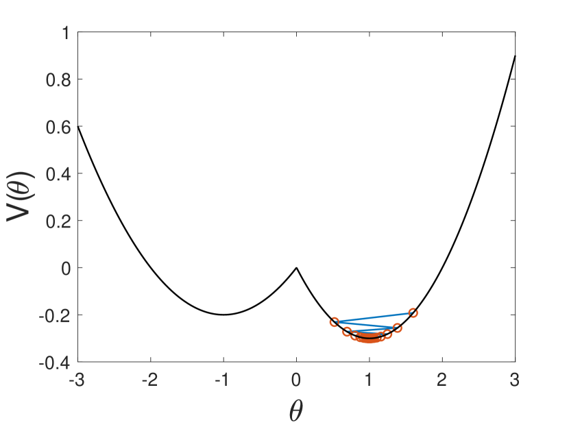
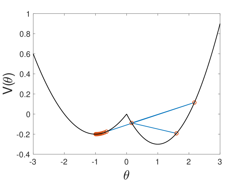
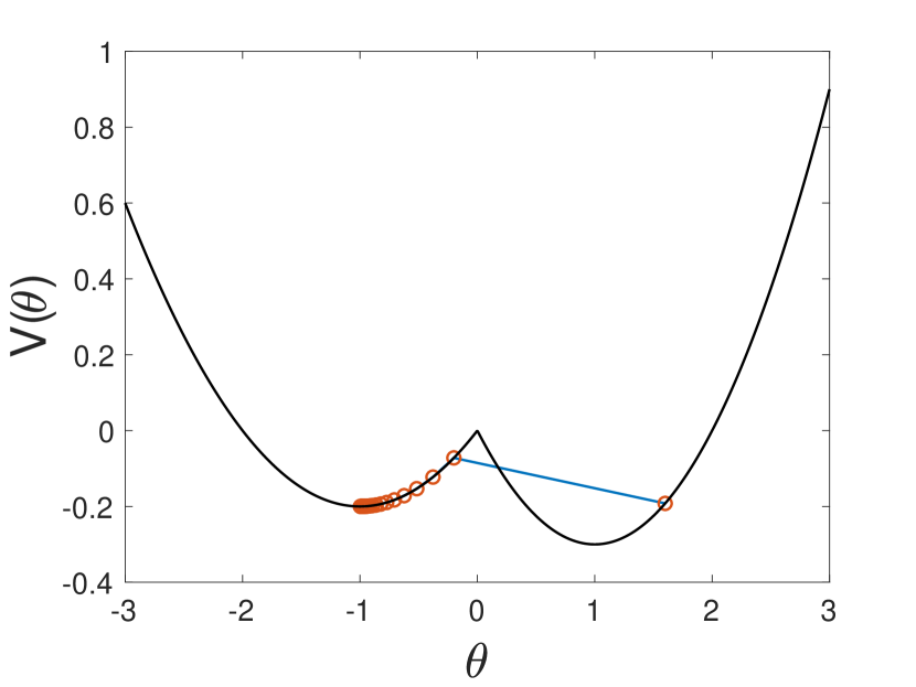
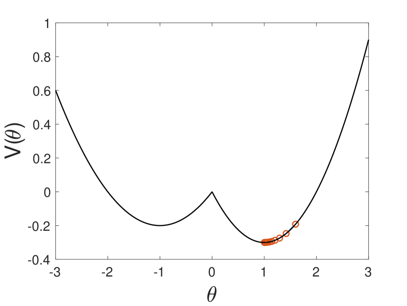
(a) $\eta$ = 0.3

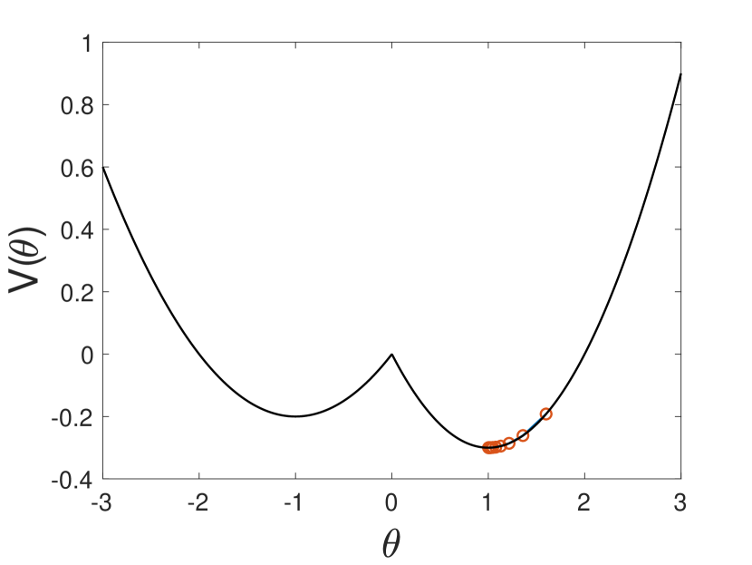
(b) $\eta$ = 0.4

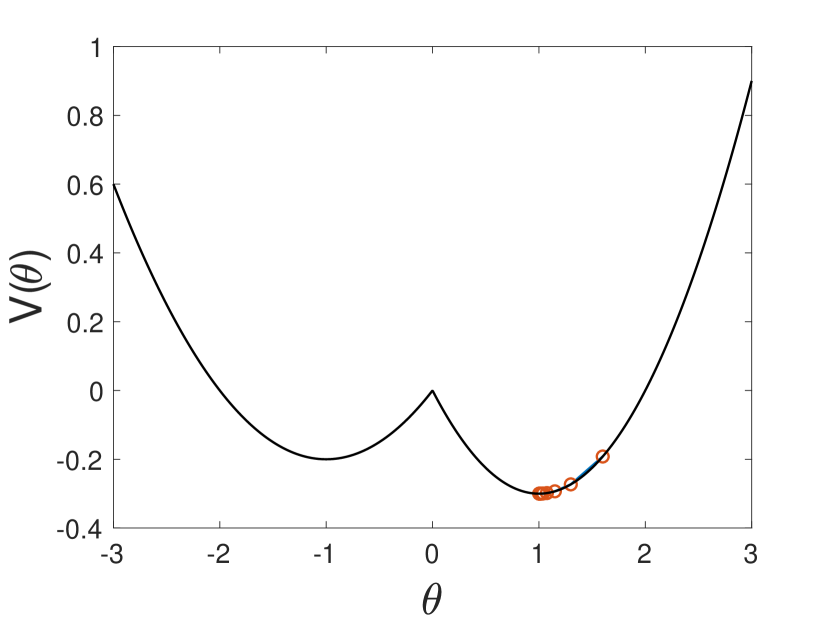
(c) $\eta$ = 0.5

(d) $\eta$ = 0.6

Figure 5: A comparison of reweighting (upper row) and resampling (lower row) with $a_{1}/a_{2}=0.4/0.6$ and $f_{1}/f_{2}=0.9/0.1$ at various learning rates $\eta$. All experiments start at $\theta_{0}=1.6$. We can see that unless the learning rate $\eta<0.4$, resampling is more stable near the minimizer $\theta=1$.

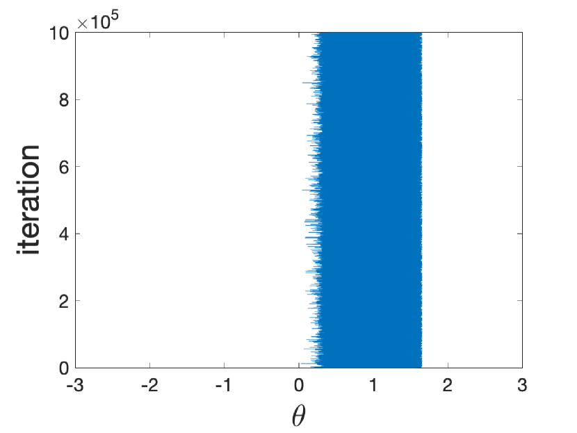
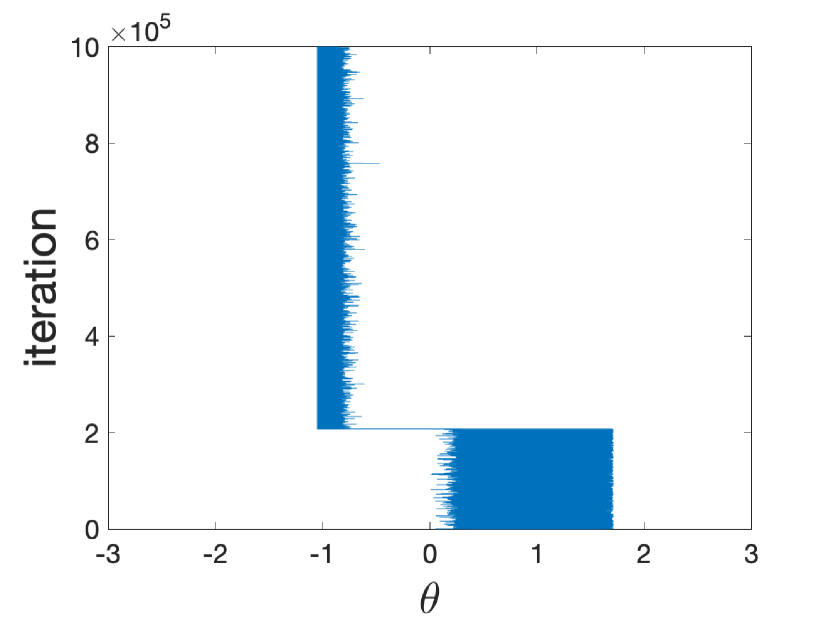
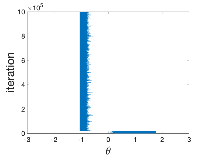
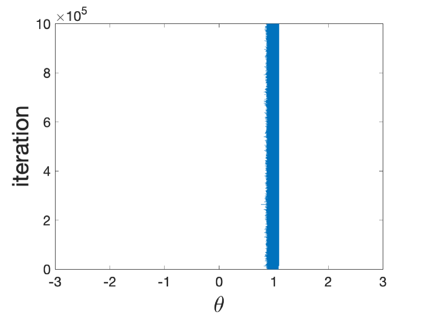
(a) $\eta$ = 0.10

(b) $\eta$ = 0.11

(c) $\eta$ = 0.12

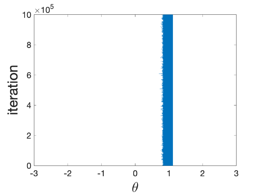
(d) $\eta$ = 0.13

Figure 6: A comparison of reweighting (upper row) and resampling (lower row) with $a_{1}/a_{2}=0.4/0.6$, $f_{1}/f_{2}=0.9/0.1$ and $\epsilon=0.1$ at various learning rates $\eta$. All experiments start at $\theta_{0}=0.9$. We can see that unless the learning rate $\eta<0.12$, resampling is more reliable in the sense that its trajectory stays around the desired minimizer.

References

- Amini et al. (2019) Alexander Amini, Ava P Soleimany, Wilko Schwarting, Sangeeta N Bhatia, and Daniela Rus. Uncovering and mitigating algorithmic bias through learned latent structure. In Proceedings of the 2019 AAAI/ACM Conference on AI, Ethics, and Society, pp. 289–295, 2019.
- Bolukbasi et al. (2016) Tolga Bolukbasi, Kai-Wei Chang, James Y Zou, Venkatesh Saligrama, and Adam T Kalai. Man is to computer programmer as woman is to homemaker? debiasing word embeddings. In Advances in neural information processing systems, pp. 4349–4357, 2016.
- Caliskan et al. (2017) Aylin Caliskan, Joanna J Bryson, and Arvind Narayanan. Semantics derived automatically from language corpora contain human-like biases. Science, 356(6334):183–186, 2017.
- Calmon et al. (2017) Flavio Calmon, Dennis Wei, Bhanukiran Vinzamuri, Karthikeyan Natesan Ramamurthy, and Kush R Varshney. Optimized pre-processing for discrimination prevention. In Advances in Neural Information Processing Systems, pp. 3992–4001, 2017.
- Chang et al. (2017) Haw-Shiuan Chang, Erik Learned-Miller, and Andrew McCallum. Active bias: Training more accurate neural networks by emphasizing high variance samples. In Advances in Neural Information Processing Systems, pp. 1002–1012, 2017.
- Galar et al. (2011) Mikel Galar, Alberto Fernandez, Edurne Barrenechea, Humberto Bustince, and Francisco Herrera. A review on ensembles for the class imbalance problem: bagging-, boosting-, and hybrid-based approaches. IEEE Transactions on Systems, Man, and Cybernetics, Part C (Applications and Reviews), 42(4):463–484, 2011.
- Guo et al. (2017) Haixiang Guo, Yijing Li, Jennifer Shang, Mingyun Gu, Yuanyue Huang, and Bing Gong. Learning from class-imbalanced data: Review of methods and applications. Expert Systems with Applications, 73:220–239, 2017.
- He & Garcia (2009) Haibo He and Edwardo A Garcia. Learning from imbalanced data. IEEE Transactions on knowledge and data engineering, 21(9):1263–1284, 2009.
- He & Ma (2013) Haibo He and Yunqian Ma. Imbalanced learning: foundations, algorithms, and applications. John Wiley & Sons, 2013.
- Kamiran & Calders (2012) Faisal Kamiran and Toon Calders. Data preprocessing techniques for classification without discrimination. Knowledge and Information Systems, 33(1):1–33, 2012.
- Kay et al. (2015) Matthew Kay, Cynthia Matuszek, and Sean A Munson. Unequal representation and gender stereotypes in image search results for occupations. In Proceedings of the 33rd Annual ACM Conference on Human Factors in Computing Systems, pp. 3819–3828, 2015.
- Kingma & Ba (2014) Diederik P Kingma and Jimmy Ba. Adam: A method for stochastic optimization. arXiv preprint arXiv:1412.6980, 2014.
- Krawczyk (2016) Bartosz Krawczyk. Learning from imbalanced data: open challenges and future directions. Progress in Artificial Intelligence, 5(4):221–232, 2016.
- Kumar et al. (2010) M Pawan Kumar, Benjamin Packer, and Daphne Koller. Self-paced learning for latent variable models. In Advances in neural information processing systems, pp. 1189–1197, 2010.
- Li et al. (2017) Qianxiao Li, Cheng Tai, and E Weinan. Stochastic modified equations and adaptive stochastic gradient algorithms. In International Conference on Machine Learning, pp. 2101–2110, 2017.
- Li et al. (2019) Qianxiao Li, Cheng Tai, and E Weinan. Stochastic modified equations and dynamics of stochastic gradient algorithms i: Mathematical foundations. J. Mach. Learn. Res., 20:40–1, 2019.
- López et al. (2013) Victoria López, Alberto Fernández, Salvador García, Vasile Palade, and Francisco Herrera. An insight into classification with imbalanced data: Empirical results and current trends on using data intrinsic characteristics. Information sciences, 250:113–141, 2013.
- Maciejewski & Stefanowski (2011) Tomasz Maciejewski and Jerzy Stefanowski. Local neighbourhood extension of smote for mining imbalanced data. In 2011 IEEE symposium on computational intelligence and data mining (CIDM), pp. 104–111. IEEE, 2011.
- Malisiewicz et al. (2011) Tomasz Malisiewicz, Abhinav Gupta, and Alexei A Efros. Ensemble of exemplar-svms for object detection and beyond. In 2011 International conference on computer vision, pp. 89–96. IEEE, 2011.
- Mani & Zhang (2003) Inderjeet Mani and I Zhang. knn approach to unbalanced data distributions: a case study involving information extraction. In Proceedings of workshop on learning from imbalanced datasets, volume 126, 2003.
- Menon et al. (2020) Sachit Menon, Alexandru Damian, Shijia Hu, Nikhil Ravi, and Cynthia Rudin. Pulse: Self-supervised photo upsampling via latent space exploration of generative models. In Proceedings of the IEEE/CVF Conference on Computer Vision and Pattern Recognition, pp. 2437–2445, 2020.
- Moro et al. (2014) Sérgio Moro, Paulo Cortez, and Paulo Rita. A data-driven approach to predict the success of bank telemarketing. Decision Support Systems, 62:22–31, 2014.
- Müller-Gronbach et al. (2020) Thomas Müller-Gronbach, Larisa Yaroslavtseva, et al. On the performance of the euler–maruyama scheme for sdes with discontinuous drift coefficient. In Annales de l’Institut Henri Poincaré, Probabilités et Statistiques, volume 56, pp. 1162–1178. Institut Henri Poincaré, 2020.
- Rotskoff & Vanden-Eijnden (2018) Grant Rotskoff and Eric Vanden-Eijnden. Parameters as interacting particles: long time convergence and asymptotic error scaling of neural networks. In Advances in neural information processing systems, pp. 7146–7155, 2018.
- Schlegel et al. (2019) Matthew Schlegel, Wesley Chung, Daniel Graves, Jian Qian, and Martha White. Importance resampling for off-policy prediction. In Advances in Neural Information Processing Systems, pp. 1799–1809, 2019.
- Seiffert et al. (2008) Chris Seiffert, Taghi M Khoshgoftaar, Jason Van Hulse, and Amri Napolitano. Resampling or reweighting: A comparison of boosting implementations. In 2008 20th IEEE International Conference on Tools with Artificial Intelligence, volume 1, pp. 445–451. IEEE, 2008.
- Shi et al. (2019) Bin Shi, Simon S Du, Weijie Su, and Michael I Jordan. Acceleration via symplectic discretization of high-resolution differential equations. In Advances in Neural Information Processing Systems, pp. 5744–5752, 2019.
- Sweeney (2013) Latanya Sweeney. Discrimination in online ad delivery. Queue, 11(3):10–29, 2013.
- Wu et al. (2018) Lei Wu, Chao Ma, and Weinan E. How sgd selects the global minima in over-parameterized learning: A dynamical stability perspective. In Advances in Neural Information Processing Systems, pp. 8279–8288, 2018.
- Zhao et al. (2019) Han Zhao, Amanda Coston, Tameem Adel, and Geoffrey J Gordon. Conditional learning of fair representations. In International Conference on Learning Representations, 2019.