Variation bounds for spherical averages

Abstract.

We consider $r$-variation operators for the family of spherical means, with special emphasis on $L^{p}\to L^{q}$ estimates.

1.  Introduction

Given a subset $E\subset\mathbb{R}$ and a family of complex valued functions $t\mapsto a_{t}$ defined on $E$, the $r$-variation of $a=\{a_{t}\}_{t\in E}$ is defined by

$$|a|_{V_{r}(E)}:=\sup_{N\in\mathbb{N}}\,\,\sup_{\begin{subarray}{c}t_{1}<\cdots<t_{N}\\ t_{j}\in E\end{subarray}}\Big{(}\sum_{j=1}^{N-1}|a_{t_{j+1}}-a_{t_{j}}|^{r}\Big{)}^{1/r}$$

for all $1\leq r<\infty$, and replacing the $\ell^{r}$-sum by a $\sup$ in the case $r=\infty$. When $E={\mathbb{R}}$ we simply use the notation $V_{r}$ for $V_{r}(\mathbb{R})$. A norm on the space $V_{r}(E)$ is given by $\|a\|_{V_{r}(E)}:=\|a\|_{\infty}+|a|_{V_{r}(E)}$. Variation norms have received considerable attention in analysis as they are used to strengthen pointwise convergence results for families of operators $\{A_{t}\}$. Of particular interest is Lépingle’s inequality on the $r$-variation of martingales for $r>2$ [29] (see also [35], [8], [21], [33]) and its consequences on families of operators in ergodic theory and harmonic analysis; see e.g. the papers [20], [21], [34], [30], [16], [31], [32], which contain many other references.

In this paper we focus on local and global $r$-variation estimates for the family of spherical averages ${A}=\{A_{t}\}_{t>0}$, given by

$$A_{t}f(x)=\int_{S^{d-1}}f(x-ty)\,\mathrm{d}\sigma(y)$$

where $\,\mathrm{d}\sigma$ denotes the normalized surface measure on the unit sphere $S^{d-1}$. By a classical result of Stein [45] ($d\geq 3$) and Bourgain [7] ($d=2$) the spherical maximal function $Sf(x):=\sup_{t>0}|A_{t}f(x)|$ defines a bounded operator on $L^{p}(\mathbb{R}^{d})$ if and only if $p>\frac{d}{d-1}$. Thus, for $p$ in this range, we have $\lim_{t\to 0}A_{t}f(x)=f(x)$ a.e. for all $f\in L^{p}({\mathbb{R}}^{d})$. A strengthening of this result can be obtained by considering the variation norm operator $V_{r}A$ given by

$$V_{r}Af(x)\equiv V_{r}{[Af]}(x):=|{Af}(x)|_{V_{r}((0,\infty))};$$

note that $V_{r}[Af](x)\geq\sup_{t}|A_{t}f(x)-A_{t_{0}}f(x)|$ for all $x\in\mathbb{R}^{d}$, $t_{0}\in{\mathbb{R}}$. In this context, Jones, Wright and one of the authors [21] obtained an almost optimal result, namely $V_{r}{A}$ is bounded on $L^{p}(\mathbb{R}^{d})$ for all $r>2$ if $\frac{d}{d-1}<p\leq 2d$, and both the condition $r>2$ and the $p$-range are sharp. In the range $p>2d$, it was shown in [21] that $V_{r}A$ is $L^{p}$ bounded if $r>p/d$, and fails to be bounded if $r<p/d$, but no information was known for the critical case $r=p/d$, $p>2d$. Here we show an endpoint result for $V_{p/d}A$ in three and higher dimensions.

Theorem 1.1.

Let $d\geq 3$, $p>2d$. Then the operator $V_{p/d}A$ is of restricted weak type $(p,p)$, i.e. maps $L^{p,1}({\mathbb{R}}^{d})$ to $L^{p,\infty}({\mathbb{R}}^{d})$.

We conjecture that a similar endpoint result holds true in two dimensions, but this remains open.

Our main focus will be on $L^{p}\to L^{q}$ results when $p<q$ for local $r$-variation operators, that is, when the variation is taken over a compact subinterval $I$ of $(0,\infty)$; without loss of generality we take $I=[1,2]$. Scaling reasons quickly reveal that one needs to consider compact intervals for $L^{p}\to L^{q}$ bounds to hold if $p<q$. While this is an interesting problem in itself, it is also motivated by a question posed by Lacey [23] concerning sparse domination for the global $V_{r}A$ operator (see also [1, Problem 3.1]). See Theorem 1.7 below.

Results for the local variation operators are meant to improve on existing $L^{p}\to L^{q}$ results for the spherical local maximal function $S^{I}f(x):=\sup_{1\leq t\leq 2}A_{t}f(x)$, which we will now review. Schlag [39] (see also [40]) showed that if $d\geq 2$ there are $L^{p}(\mathbb{R}^{d})\to L^{q}(\mathbb{R}^{d})$ bounds if $(1/p,1/q)$ lies in the interior of ${\mathfrak{Q}}_{d}$, which denotes the quadrangle formed by the vertices

$$Q_{1}=(0,0), Q_{2} =(\tfrac{d-1}{d},\tfrac{d-1}{d}),$$ (1.1)

$$Q_{3}=(\tfrac{d-1}{d},\tfrac{1}{d}), Q_{4} =(\tfrac{d(d-1)}{d^{2}+1},\tfrac{d-1}{d^{2}+1}).$$

Moreover, $S^{I}$ fails to be bounded from $L^{p}(\mathbb{R}^{d})$ to $L^{q}(\mathbb{R}^{d})$ outside the closure of ${\mathfrak{Q}}_{d}$. Note that $Q_{2}$ coincides with $Q_{3}$ when $d=2$, so the quadrangle becomes a triangle in two dimensions.

The boundary segment $p=q$ amounts to the classical results of Stein and Bourgain for $S$. $L^{p}$-boundedness fails at the endpoint $Q_{2}$ but Bourgain showed in dimensions $d\geq 3$ that $S$ is of restricted weak type at $Q_{2}$, i.e. bounded from $L^{\frac{d}{d-1},1}$ to $L^{\frac{d}{d-1},\infty}$ in dimensions $d\geq 3$ (and any better Lorentz estimate fails). The restricted weak type estimate at $Q_{2}$ fails in two dimensions [42] (even though it is true for radial functions [24]). For the remaining boundary cases Lee [25] showed that $S^{I}$ is of restricted weak type at $Q_{4}$, and also at $Q_{3}$ in dimensions $d\geq 3$. The two-dimensional restricted weak type endpoint result at $Q_{4}$ was also shown in [25], and relied on the deep work by Tao [47] on endpoint bilinear Fourier extension bounds for the cone. The restricted weak type inequalities imply $L^{p}\to L^{q}$ boundedness on $[Q_{1},Q_{4})$ and on $(Q_{3},Q_{4})$, however on $(Q_{2},Q_{3})$ the operator is of restricted strong type and no better (the necessity follows from the standard counterexample; for the positive result one uses real interpolation on a vertical line, with a constant target exponent). Incidentally, for the local operator $S^{I}$ this also implies restricted strong type at $Q_{2}$, which improves over the restricted weak type of $S$ at $Q_{2}$.

Here we explore the existence of $L^{p}(\mathbb{R}^{d})\to L^{q}(\mathbb{R}^{d})$ inequalities for

$$V_{r}^{I}Af(x):=|Af(x)|_{V_{r}([1,2])}.$$

In two dimensions the values of $r$ are restricted to $r>2$ (see §3) but in higher dimensions all $r\in[1,\infty]$ may occur. For our sparse domination inequality for the global $V_{r}$, the version for $r>2$ is most relevant because Lépingle’s result requires the restriction $r>2$ (see [37]); indeed this necessary condition can be shown to carry over to other results for the global $V_{r}$.

We start stating our results for $d\geq 3$. We first focus on the range $r>\frac{d^{2}+1}{d(d-1)}$ which is the reciprocal of the $1/p$ coordinate of the point $Q_{4}$ in (1.1). Note that this large range includes $r>2$, so the following sharp $L^{p}\to L^{q}$ results for $V_{r}^{I}A$ will yield, in particular, satisfactory results for the sparse domination problem in dimension $d\geq 3$.

Theorem 1.2.

Suppose $d\geq 3$ and $r>\frac{d^{2}+1}{d(d-1)}$. Let ${\mathfrak{P}}_{d}(r)$ be the pentagon (Figure 1) with vertices

$$P(r)=(\tfrac{1}{r},\tfrac{1}{rd}),\quad Q_{1}(r)=(\tfrac{1}{rd},\tfrac{1}{rd}),\quad Q_{2}=(\tfrac{d-1}{d},\tfrac{d-1}{d})$$

$$\qquad\quad Q_{3}=(\tfrac{d-1}{d},\tfrac{1}{d}),\quad Q_{4}=(\tfrac{d(d-1)}{d^{2}+1},\tfrac{d-1}{d^{2}+1}).$$

Then

(i) $V_{r}^{I}A:L^{p}\to L^{q}$ is bounded for all $(\tfrac{1}{p},\tfrac{1}{q})$ in the interior of ${\mathfrak{P}}_{d}(r)$ and unbounded for all $(\tfrac{1}{p},\tfrac{1}{q})\notin{\mathfrak{P}}_{d}(r)$.

(ii) $V_{r}^{I}A:L^{p}\to L^{q}$ is bounded for all $(\tfrac{1}{p},\tfrac{1}{q})$ on the half open line segment $[Q_{1}(r),Q_{2})$, on the closed line segment $[P(r),Q_{1}(r)]$, on the half open line segment $[P(r),Q_{4})$, and on the open line segment $(Q_{4},Q_{3})$.

(iii) $V_{r}^{I}A:L^{p,1}\to L^{q}$ is bounded (i.e. of restricted strong type $(p,q)$) if $(\tfrac{1}{p},\tfrac{1}{q})$ belongs to the half open line segment $[Q_{2},Q_{3})$. $V_{r}^{I}A$ fails to be of strong type on $[Q_{2},Q_{3}]$.

(iv) $V_{r}^{I}A:L^{p,1}\to L^{q,\infty}$ is bounded (i.e. of restricted weak type $(p,q)$) if $(\tfrac{1}{p},\tfrac{1}{q})\in\{Q_{3},\,Q_{4}\}$.

For an explicit description of the various conditions at the boundary see §3.1.

Figure 1. The pentagon $\mathfrak{P}_{d}(r)$ for $r>\frac{d^{2}+1}{d^{2}-d}$ and $d\geq 3$ (Theorem 1.2). The outer (dashed) quadrangle shows the region of boundedness as $r\to\infty$, i.e. for the maximal operator. Shown with $d=4$ and $r=3$.

We leave open what exactly happens at the points $Q_{3}$ and $Q_{4}$; it is not even known whether the local maximal function is of restricted strong type at $Q_{3}$ and whether it is any better than restricted weak type at $Q_{4}$. If we take $r=\infty$ we recover the known theorem for the local spherical maximal operator. Note that both $P(r)$ and $Q_{1}(r)$ tend to $Q_{1}=(0,0)$ as $r\to\infty$.

Theorem 1.2 covers an interesting consequence for a sharp strong type estimate at the lower edge $q^{-1}=p^{-1}/d$ of the type set for the maximal function.

Corollary 1.3.

Let $d\geq 3$ and let $\frac{d^{2}+1}{d(d-1)}<p<\infty$. Then $V^{I}_{r}A:L^{p}\to L^{pd}$ is bounded if and only if $r\geq p$.

When the value of $r$ is between the reciprocal of the $1/p$ coordinate of $Q_{4}$ and $Q_{3}$, that is, $\tfrac{d}{d-1}<r\leq\tfrac{d^{2}+1}{d(d-1)}$, we obtain the following.

Theorem 1.4.

Suppose $d\geq 3$ and $\frac{d}{d-1}<r\leq\frac{d^{2}+1}{d(d-1)}$. Let ${\mathfrak{P}}_{d}(r)$ be the pentagon (Figure 2) with vertices

$$Q_{1}(r)=\big{(}\tfrac{1}{rd},\tfrac{1}{rd}\big{)},\quad Q_{2}=\big{(}\tfrac{d-1}{d},\tfrac{d-1}{d}\big{)},\quad Q_{3}=\big{(}\tfrac{d-1}{d},\tfrac{1}{d}\big{)}$$

$$P(r)=\big{(}\tfrac{1}{r},\tfrac{d+1-r(d-1)}{r(d-1)}\big{)},\quad Q_{4}(r)=(1-\tfrac{d+1}{rd(d-1)},\tfrac{1}{rd}).$$

Then

(i) $V_{r}^{I}A:L^{p}\to L^{q}$ is bounded for $(\tfrac{1}{p},\tfrac{1}{q})$ in the interior of ${\mathfrak{P}}_{d}(r)$ and unbounded for $(\tfrac{1}{p},\tfrac{1}{q})\notin{\mathfrak{P}}_{d}(r)$.

(ii) $V_{r}^{I}A:L^{p}\to L^{q}$ is bounded for $(\tfrac{1}{p},\tfrac{1}{q})$ on the half open line segment $(Q_{4}(r),Q_{1}(r)]$ and on the half open line segment $[Q_{1}(r),Q_{2})$.

(iii) $V_{r}^{I}A$ is of restricted strong type $(p,q)$ if $(\tfrac{1}{p},\tfrac{1}{q})$ belongs to the half open line segment $[Q_{2},Q_{3})$. $V_{r}^{I}A$ fails to be of strong type on $[Q_{2},Q_{3}]$.

(iv) $V_{r}^{I}A$ is of restricted weak type $(p,q)$ if $(\tfrac{1}{p},\tfrac{1}{q})=Q_{3}$.

Note that for $r=\tfrac{d^{2}+1}{d(d-1)}$ the pentagon ${\mathfrak{P}}_{d}(r)$ in Figure 2 degenerates to a quadrangle, as $P(r)=Q_{4}(r)=Q_{4}$. We leave open what happens at the closed boundary segment $[Q_{4}(r),P(r)]$ and the half-open boundary segment $[P(r),Q_{3})$.

Figure 2. The pentagon $\mathfrak{P}_{d}(r)$ for $\frac{d}{d-1}<r\leq\frac{d^{2}+1}{d^{2}-d}$ and $d\geq 3$ (Theorem 1.4). The outer (dashed) quadrangle is the region of boundedness for the maximal operator. Shown with $d=4$ and $r=\frac{11}{8}$.

Figure 3. The quadrangle $\mathfrak{Q}_{d}(r)$ for $1\leq r\leq\frac{d}{d-1}$ and $d\geq 4$ (Theorem 1.5). The outer (dashed) quadrangle is the boundedness region for the maximal function. Shown with $d=4$ and $r=\frac{5}{4}$.

Finally, we address small values of $r$.

Theorem 1.5.

Suppose that either $d\geq 4$ and $1\leq r\leq\tfrac{d}{d-1}$ or $d=3$ and $\tfrac{4}{3}<r\leq\tfrac{3}{2}$. Let ${\mathfrak{Q}}_{d}(r)$ be the quadrangle (Figure 3) with vertices

$$Q_{1}(r)=\big{(}\tfrac{1}{rd},\tfrac{1}{rd}\big{)},\quad Q_{2}(r)=\big{(}\tfrac{r(d-1)-1}{r(d-1)},\tfrac{r(d-1)-1}{r(d-1)}),$$

$$Q_{3}(r)=(\tfrac{r(d-1)-1}{r(d-1)},\tfrac{1}{r(d-1)}),\quad Q_{4}(r)=(1-\tfrac{d+1}{rd(d-1)},\tfrac{1}{rd}).$$

Then

(i) $V_{r}^{I}A:L^{p}\to L^{q}$ is bounded for $(\tfrac{1}{p},\tfrac{1}{q})$ in the interior of ${\mathfrak{Q}}_{d}(r)$ and unbounded for $(\tfrac{1}{p},\tfrac{1}{q})\notin{\mathfrak{Q}}_{d}(r)$.

(ii) $V_{r}^{I}A:L^{p}\to L^{q}$ is bounded if $(\frac{1}{p},\frac{1}{q})$ is in the half open line segment $(Q_{4}(r),Q_{1}(r)]$ and $[Q_{1}(r),Q_{2}(r))$.

(iii) For the case $r=1$, $d\geq 4$, the operator $V_{1}^{I}A$ is of restricted weak type $(\tfrac{d-1}{d-2},d-1)$ (that is, at $Q_{3}(1)$) and of restricted strong type $(\tfrac{d-1}{d-2},q)$ for $\tfrac{d-1}{d-2}\leq q<d-1$ (that is, on $[Q_{2}(1),Q_{3}(1))$). In three dimensions, $V_{1}^{I}A:L^{2}({\mathbb{R}}^{3})\to L^{2}({\mathbb{R}}^{3})$ is bounded.

We leave open what happens at the closed boundary segments $[Q_{2}(r),Q_{3}(r)]$ for $1<r\leq\frac{d}{d-1}$ and $[Q_{3}(r),Q_{4}(r)]$ for $1\leq r\leq\frac{d}{d-1}$.

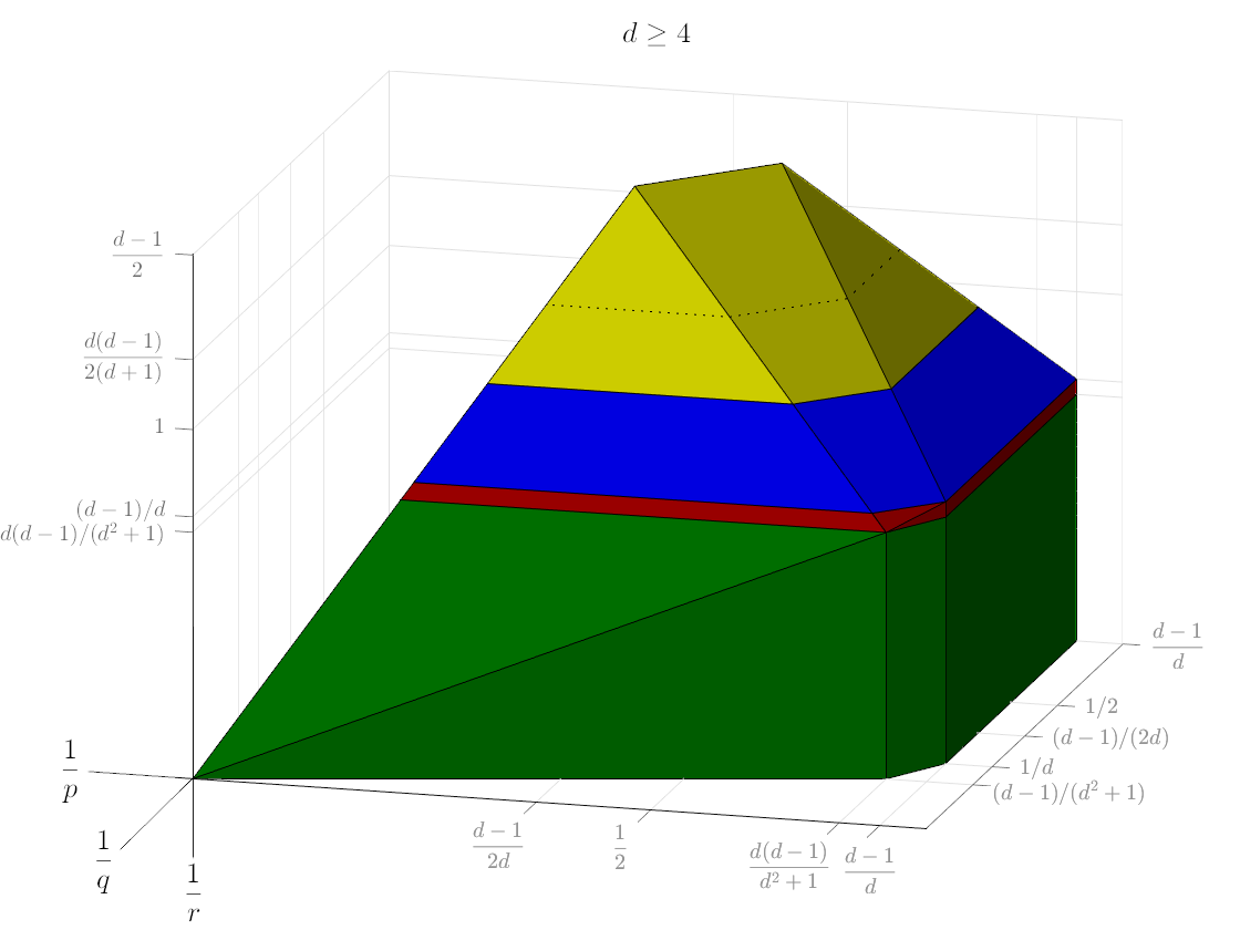
Figure 4. A diagram of the typeset of $V_{r}^{I}A$ in $(\frac{1}{p},\frac{1}{q},\frac{1}{r})$-space for large values of $d$. The green region corresponds to Theorem 1.2 (Figure 1), the red region corresponds to Theorem 1.4 (Figure 2), and the blue region corresponds to Theorem 1.5 (Figure 3). The yellow region is conjectural.

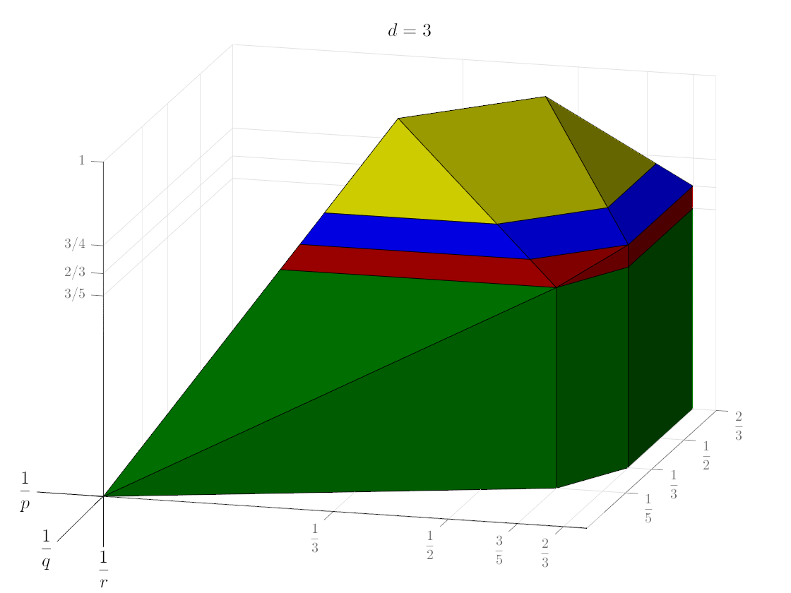
Figure 5. A diagram of the typeset of $V_{r}^{I}A$ in $(\frac{1}{p},\frac{1}{q},\frac{1}{r})$-space for $d=3$. The green region corresponds to Theorem 1.2 (Figure 1), the red region corresponds to Theorem 1.4 (Figure 2), and the blue region corresponds to Theorem 1.5 (Figure 3). The yellow region is conjectural.

Note that there is a discrepancy in our results between $d=3$, for which we only obtain sharp results in the partial range $\frac{4}{3}<r\leq\frac{d}{d-1}$ and the case $d\geq 4$, where results are obtained for all $1\leq r\leq\frac{d}{d-1}$. The reason is because we restrict ourselves to the traditional range $1\leq r\leq\infty$ for the variation norm. The definition of $V_{r}$ can be extended, with modifications, to the range $0<r<1$ (see for example [4]). In that context, one can formulate conjectural results for $V_{r}^{I}A$ for $\frac{2}{d-1}<r<1$ (see Figure 4) for $d\geq 4$. We remark that a positive solution to Sogge’s local smoothing conjecture [43] in $d+1$ dimensions would imply a complete result up to endpoints. Partial results in the range $r>\frac{2(d+1)}{d(d-1)}$ can be proved using the techniques of this paper. We shall address issues for $r<1$ in a follow up paper.

Similarly, in three dimensions, the range $1\leq r\leq 4/3$ remains open as a conjecture (see Figure 5). Note that here we are in the traditional range for the $V_{r}$ spaces.

In dimension 2, due to the recent full resolution of Sogge’s problem in $2+1$ dimensions by Guth, Wang and Zhang [17], that is,

$$\partial_{t}^{1/2-\varepsilon}A:L^{4}\to L^{4}(L^{4}),$$

it is possible to get an almost optimal result (up to endpoints) for the variation norm estimates.

Theorem 1.6.

Let $d=2$.

(i) If $r>5/2$ then $V_{r}^{I}A:L^{p}\to L^{q}$ is bounded if $(\tfrac{1}{p},\tfrac{1}{q})$ is either in the interior of the quadrangle ${\mathfrak{Q}}_{2}(r)$ (Figure 6) formed by the vertices

$$P(r)=(\tfrac{1}{r},\tfrac{1}{2r}),\quad Q_{1}(r)=(\tfrac{1}{2r},\tfrac{1}{2r}),$$

$$Q_{2}=Q_{3}=(\tfrac{1}{2},\tfrac{1}{2}),\quad Q_{4}=(\tfrac{2}{5},\tfrac{1}{5})$$

or in the open line segment between $Q_{2}=Q_{3}$ and $Q_{1}(r)$.

(ii) If $2<r\leq 5/2$ then $V_{r}^{I}A:L^{p}\to L^{q}$ is bounded if $(\tfrac{1}{p},\tfrac{1}{q})$ is either in the interior of the quadrangle ${\mathfrak{Q}}_{2}(r)$ (Figure 7) formed by the vertices

$$Q_{1}(r)=\big{(}\tfrac{1}{2r},\tfrac{1}{2r}\big{)},\quad Q_{2}=Q_{3}=\big{(}\tfrac{1}{2},\tfrac{1}{2}),$$

$$P(r)=(\tfrac{1}{r},\tfrac{3-r}{r}),\quad Q_{4}(r)=(1-\tfrac{3}{2r},\tfrac{1}{2r})$$

or in the open line segment between $Q_{2}=Q_{3}$ and $Q_{1}(r)$.

(iii) If $r<2$ then $V_{r}^{I}A$ does not map any $L^{p}({\mathbb{R}}^{2})$ to any $L^{q}({\mathbb{R}}^{2})$.

Figure 6. The region ${\mathfrak{Q}}_{2}(r)$ if $r>5/2$ (Theorem 1.6 i). The outer (dashed) triangle is the region of boundedness for the maximal operator. Shown with $r=5$.

Note that, as for the circular maximal function theorem, the points $Q_{2}$ and $Q_{3}$ coincide if $d=2$; therefore the pentagon (Figures 1 and 2) in Theorems 1.2 and 1.4 becomes a quadrangle for $r>2$. Moreover, $P(5/2)=Q_{4}(5/2)=Q_{4}$, so the quadrangle becomes a triangle for $r=5/2$. The bounds are subsumed in Figure 8; note that in contrast with $d\geq 3$, the blue/yellow region disappears, as $\frac{d}{d-1}=\frac{2}{d-1}$ coincide for $d=2$.

It is also possible to show unboundedness for $r=2$ via an argument involving the Besicovitch set, which will be addressed in a forthcoming paper.

We note that an affirmative answer to endpoint versions of Sogge’s problem as formulated and conjectured in [18] would also settle strong type bounds on the half-open boundary segment $(Q_{4}(r),Q_{1}(r)]$. Unfortunately such endpoint bounds in Sogge’s problem are currently only available in dimensions four and higher.

Figure 7. The region ${\mathfrak{Q}}_{2}(r)$ if $d=2$ and $2<r\leq 5/2$ (Theorem 1.6 ii). The outer (dashed) triangle is the region of boundedness for the maximal operator. Shown with $r=2.2$.

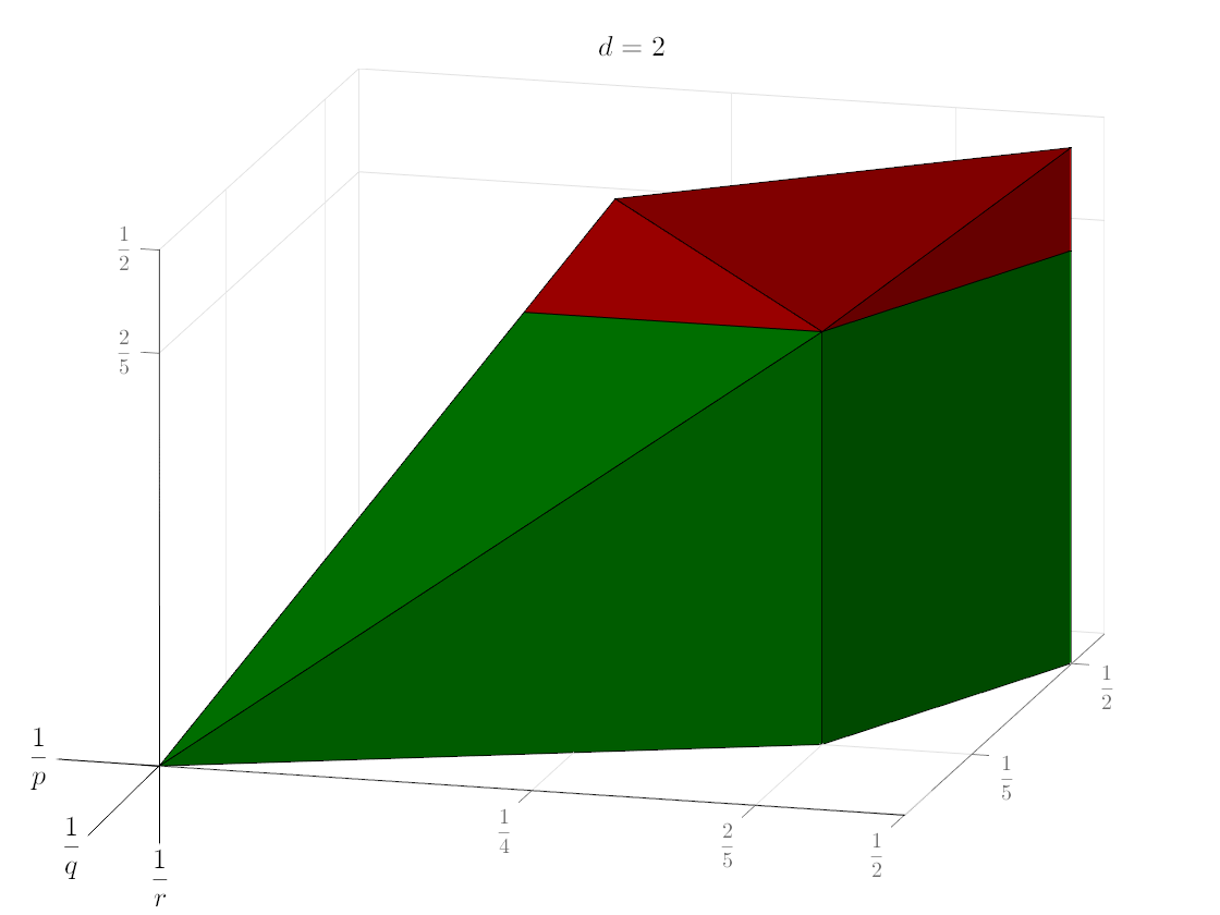
Figure 8. A diagram of the typeset of $V_{r}^{I}A$ in $(\frac{1}{p},\frac{1}{q},\frac{1}{r})$-space for $d=2$. The green region corresponds to Figure 6 and the red region corresponds to Figure 7.

Sparse domination

We now formulate a sparse domination result for the global operator $V_{r}A$, $r>2$. Recall that a family of cubes $\mathfrak{S}$ in $\mathbb{R}^{d}$ is called sparse if for every $Q\in{\mathfrak{S}}$ there is a measurable subset $E_{Q}\subset Q$ such that $|E_{Q}|\geq|Q|/2$ and such that the sets on the family $\{E_{Q}:Q\in{\mathfrak{S}}\}$ are pairwise disjoint. In what follows we abbreviate $\langle f\rangle_{Q,s}=(|Q|^{-1}\int_{Q}|f|^{s})^{1/s}.$

Theorem 1.7.

Assume one of the following holds:

1. $d\geq 3$, $r>2$, and $(\tfrac{1}{p},\tfrac{1}{q})$ in the interior of ${\mathfrak{P}}_{d}(r)$.

2. $d=2$, $r>2$ and $(\tfrac{1}{p},\tfrac{1}{q})$ in the interior of ${\mathfrak{Q}}_{2}(r)$.

Then there is a constant $C=C(p,q)$ such that for each pair of compactly supported bounded functions $f_{1}$, $f_{2}$ there is a sparse family of cubes $\mathfrak{S}$ such that

$$\int_{\mathbb{R}^{d}}V_{r}Af_{1}(x)f_{2}(x)\,\mathrm{d}x\leq C\sum_{Q\in\mathfrak{S}}|Q|\langle f_{1}\rangle_{Q,p}\langle f_{2}\rangle_{Q,q^{\prime}},$$ (1.2)

where $\frac{1}{q}+\frac{1}{q^{\prime}}=1$. Furthermore, the $(1/p,1/q)$ range is sharp up to endpoints in the sense that no such result can hold if $(1/p,1/q)$ does not lie in the closure of ${\mathfrak{P}}_{d}(r)$, or ${\mathfrak{Q}}_{2}(r)$, respectively.

Theorem 1.7 can be obtained as an immediate consequence of a (more general) sparse domination result in [2], together with the $L^{p}$ results in [21] and Theorems 1.2 and 1.6; see §3.9 and §8. Sparse domination is known to imply as a corollary a number of weighted inequalities in the context of Muckenhoupt and reverse Hölder classes. We refer the interested reader to [5] for the weighted consequences for $V_{r}A$ of Theorem 1.7.

Overview of the argument

Our positive results can be classified in the following 4 groups of estimates:

• The $L^{p}\to L^{q}$ bounds for $V_{r}^{I}$ in the interior of the regions in Theorems 1.2, 1.4, 1.5 and 1.6. These can all be obtained from a single scale frequency analysis. More precisely, for a triple $(p,q,r)$, one obtains bounds which decay geometrically with respect to the frequency scale. By a Besov space embedding, these can be obtained from suitable space-time $L^{p}\to L^{q}(L^{r})$ bounds for the spherical averages $A_{t}$, which in turn follow from interpolation (and a localization argument) among the basic estimates $L^{1}\to L^{\infty}(L^{1}),L^{2}\to L^{2}(L^{2})$, $L^{\infty}\to L^{\infty}(L^{\infty})$ and $L^{1}\to L^{1}(L^{1})$ together with key local smoothing estimates, such as the Guth–Wang–Zhang [17] result for $d=2$, or a Stein–Tomas type estimate for $d\geq 3$.

• The Lebesgue space bounds for $V_{r}^{I}$ at certain boundaries of the regions in Theorems 1.2, 1.4, 1.5 and 1.6. Except for $q=rd$ and the segment $[P(r),Q_{4}]$ in Theorem 1.2, the remaining claimed estimates along the boundary can be obtained by combining the single scale frequency bounds from the previous item and Bourgain’s interpolation argument.

• The $L^{p}\to L^{q}$ bounds for $V_{r}^{I}$ at the boundary segment with $q=rd$ in Theorems 1.2, 1.4, 1.5. These estimates are harder to obtain and require a more delicate analysis. In contrast to the previous cases, we use a multi-scale frequency analysis and the Fefferman–Stein sharp maximal function. Effective bounds follow from exploiting cancellation, the local nature of the estimates, and a careful real interpolation of certain localised pieces. This also subsumes the boundary segment $[P(r),Q_{4}]$ in Theorem 1.2 and Corollary 1.3.

• The restricted weak type estimate for $V_{p/d}$ in Theorem 1.1. Again, this estimate is of a harder nature. In view of the better bounds satisfied by the long variation operator, which were proven in [21], it suffices to prove the endpoint bound for the so-called short variation operator, which corresponds to the $\ell^{r}(\mathbb{Z})$-norm of the map $k\to V_{r}^{I_{k}}A$, where $I_{k}=[2^{k},2^{k+1}]$. We perform a single scale in frequency but a multi-scale in time analysis, for which we combine the previous techniques. In particular, we use the Fefferman–Stein maximal function to deal with multi-scale time sums and prove estimates for single frequency pieces of the short variation operator. These can then be combined with Bourgain’s interpolation argument to obtain the desired endpoint result.

Structure of the paper

We start gathering some well known facts about spherical averages and function spaces in §2. In §3 we provide the examples showing the necessary conditions for our theorems. In §4 we exploit the single frequency analysis to deduce the claimed bounds in the interior of the regions, as well as some restricted weak and strong type endpoints, in Theorems 1.2, 1.4, 1.5 and 1.6. The proof of the harder off-diagonal strong type boundary results in those theorems, and therefore Corollary 1.3, is provided in §§5-6. In §7 we prove the restricted weak type inequality for the global operator in Theorem 1.1. Finally, the sparse domination result is discussed in §8.

Acknowledgements

We are indebted to Shaoming Guo for useful contributions at various stages of the project. Some initial work on this project was done during the workshop “Sparse domination of singular integral operators” in October 2017, attended by four of the authors. We would like to thank the American Institute of Mathematics for hosting the workshop, as well as the organizers Amalia Culiuc, Francesco Di Plinio and Yumeng Ou. D.B. was partially supported by the NSF grant DMS-1954479. L.R. was partially supported by the Basque Government through the BERC 2018-2021 program, by the Spanish Ministry of Economy and Competitiveness: BCAM Severo Ochoa excellence accreditation SEV-2017-2018 and through project MTM2017-82160-C2-1-P, by the project RYC2018-025477-I, and by Ikerbasque. A.S. was partially supported by NSF grant DMS-1764295 and by a Simons fellowship. B.S. was partially supported by NSF grant DMS-1653264.

2.  Preliminaries

It will be convenient to consider the $t$-parameter as a variable. To this end, let $\chi\in C^{\infty}_{c}({\mathbb{R}})$ so that $\chi(t)=1$ for $t$ in a neighborhood of $[1,2]$ and supported in $[1/2,4]$, and define

$${\mathcal{A}}f(x,t):=\chi(t)A_{t}f(x).$$ (2.1)

In view of future frequency decompositions, let $\beta_{0}\in C^{\infty}_{c}({\mathbb{R}})$ so that $\beta_{0}(s)=1$ for $|s|<1/2$ and $\beta_{0}(s)=0$ for $|s|>1$. For every integer $j\geq 1$, set

$$\beta_{j}(s)=\beta_{0}(2^{-j}s)-\beta_{0}(2^{1-j}s).$$

For functions $g$ on ${\mathbb{R}}$, and $l\in\mathbb{N}_{0}$, define the operators $\Lambda_{l}$ by

$$\widehat{\Lambda_{l}g}(\tau)=\beta_{l}(\tau)\widehat{g}(\tau).$$ (2.2)

For functions $f$ on $\mathbb{R}^{d}$, and $j\in\mathbb{N}_{0}$, define the operators $L_{j}$ by

$$\widehat{L_{j}f}(\xi)=\beta_{j}(|\xi|)\widehat{f}(\xi),$$ (2.3)

and let $\widetilde{L}_{j}$ be a modification of $L_{j}$ satisfying $\widetilde{L}_{j}L_{j}=L_{j}$.

2.1.  $V_{r}$ and related function spaces

It will be convenient to work with the Besov space $B^{1/r}_{r,1}$. The Besov spaces $B^{s}_{p,q}({\mathbb{R}})$ can be defined using the dyadic frequency decompositions $\{\Lambda_{l}\}_{l=0}^{\infty}$ on the real line and we have $\|u\|_{B^{s}_{p,q}}=(\sum_{l=0}^{\infty}[2^{ls}\|\Lambda_{l}u\|_{L^{p}}]^{q})^{1/q}$. From the Plancherel–Pólya inequality we know the embedding

$$B^{1/r}_{r,1}\hookrightarrow V_{r}\hookrightarrow B^{1/r}_{r,\infty},\quad$$ (2.4)

see [48, Ch.1]. One can also consult the paper by Bergh and Peetre [4] (who however work with a different type of variation space when $r=1$) or refer to [16, Proposition 2.2]. Thus an inequality for the variation operator $V_{r}^{I}{\mathcal{A}}$ follows if we can control the $B^{1/r}_{r,1}$ norm of $t\mapsto{\mathcal{A}}f(x,t)$.

Note that, by our definition, $V_{1}(\mathbb{R})$ coincides with the space of bounded functions of bounded variations. The fundamental theorem of calculus implies

$$\|V_{1}^{E}A\|_{L^{p}\to L^{q}}\leq\|\partial_{t}\mathcal{A}\|_{L^{p}\to L^{q}(L^{1}(E))},$$ (2.5)

so we shall focus on obtaining bounds for the right-hand side when studying $V_{1}^{E}A$.

2.2.  Frequency decomposition in space

Given $j\geq 0$, write

$$A_{t}L_{j}f=K_{j,t}*f,$$ (2.6)

where $L_{j}$ is as in (2.3), so that $\widehat{K_{j,t}}(\xi)=\widehat{\sigma}(t\xi)\beta_{j}(|\xi|)$. Note that $K_{j,t}$ is a Schwartz convolution kernel and therefore we restrict our attention to the case $j\geq 1$.

An immediate computation yields the following pointwise estimates for the convolution kernel.

Lemma 2.1.

For all $N\in\mathbb{N}_{0}$, there exists a constant $C_{N}>0$ such that

$$|\partial_{t}^{\varsigma}K_{j,t}(x)|\lesssim_{\varsigma}C_{N}2^{j\varsigma}\frac{2^{j}}{(1+2^{j}\big{|}|x|-t\big{|})^{N}}$$ (2.7)

holds for all $x\in\mathbb{R}^{d}$, all $t>0$ and all $\varsigma\in\mathbb{N}_{0}$. Consequently,

$$|K_{j,t}(x)|\lesssim_{N}(2^{j}|x|)^{-N}\qquad\text{ if}\quad|x|\geq 10,\quad t\in[1/2,4].$$ (2.8)

In analogy to the definition of ${\mathcal{A}}$ in (2.1), define

$${\mathcal{A}}_{j}f(x,t):=\chi(t)A_{t}L_{j}f(x)=\chi(t)K_{j,t}*f(x).$$

We gather some estimates for ${\mathcal{A}}_{j}$ when the inequalities involve $L^{1}$ or $L^{\infty}$ spaces.

First, from the trivial fact that $\|A_{t}f\|_{L^{\infty}}\lesssim\|f\|_{L^{\infty}}$ uniformly in $t\in\mathbb{R}$, one immediately has

$$\|\mathcal{A}_{j}f\|_{L^{\infty}(L^{\infty})}\lesssim\|f\|_{L^{\infty}}.$$ (2.9)

Moreover, one has the following estimates for $L^{1}$ functions.

Lemma 2.2.

For $1\leq q\leq\infty$,

$$\|{\mathcal{A}}_{j}f\|_{L^{q}(L^{1})}+2^{-j}\|\partial_{t}{\mathcal{A}}_{j}f\|_{L^{q}(L^{1})}\lesssim\|f\|_{L^{1}}.$$

Proof.

By (2.7) one has

$$\big{|}{\mathcal{A}}_{j}f(x,t)\big{|}+2^{-j}\big{|}\partial_{t}{\mathcal{A}}_{j}f(x,t)\big{|}\lesssim\int_{\mathbb{R}^{d}}|f(y)|\frac{2^{j}}{(1+2^{j}||x-y|-t|)^{N}}\,\,\mathrm{d}y$$ (2.10)

for all $N\in\mathbb{N}_{0}$. Integrating in $t$ over the support of $\chi$ one sees that, for fixed $x$,

$$\int_{1/2}^{4}\big{|}{\mathcal{A}}_{j}f(x,t)\big{|}\,\mathrm{d}t+2^{-j}\int_{1/2}^{4}\big{|}\partial_{t}{\mathcal{A}}_{j}f(x,t)\big{|}\,\mathrm{d}t$$

$$\lesssim\int_{\mathbb{R}^{d}}|f(y)|\int_{1/2}^{4}\frac{2^{j}}{(1+2^{j}||x-y|-t|)^{N}}\,\mathrm{d}t\,\,\mathrm{d}y\,\lesssim\|f\|_{L^{1}}.$$

This gives the assertion for $q=\infty$.

For $q=1$, the result follows from integrating in $x$ instead, using the decay in (2.10) and taking into account that the integration in $t$ is over $[1/2,4]$.

The remaining cases $1<q<\infty$ follow from combining the above through Young’s convolution inequality. ∎

Corollary 2.3.

For $1\leq r\leq\infty,$

$$\|{\mathcal{A}}_{j}f\|_{L^{\infty}(L^{r})}\lesssim 2^{j(1-\frac{1}{r})}\|f\|_{L^{1}}.$$

Proof.

Interpolate between

$$\|{\mathcal{A}}_{j}\|_{L^{\infty}(L^{\infty})}\lesssim 2^{j}\|f\|_{L^{1}},$$

which follows from (2.7), and Lemma 2.2 with $q=\infty$. ∎

2.3.  Oscillatory integral representation

Given $m\in\mathbb{R}$, let $S^{m}(\mathbb{R}^{d})$ denote the class of all functions $a\in C^{\infty}(\mathbb{R}^{d})$ satisfying

$$|\partial^{\alpha}a(\xi)|\lesssim_{\alpha}(1+|\xi|)^{m-|\alpha|}$$

for all multiindex $\alpha\in\mathbb{N}_{0}^{d}$ and all $\xi\in\mathbb{R}^{d}$. Given $a\in S^{m}(\mathbb{R})$, define

$$T_{j}^{\pm}[a,f](x,t)=\int_{\mathbb{R}^{d}}\beta_{j}(|\xi|)a(t|\xi|)e^{i\langle x,\xi\rangle\pm it|\xi|}\widehat{f}(\xi)\,\mathrm{d}\xi.$$ (2.11)

It is well known that the Fourier transform of the spherical measure is

$$\widehat{\sigma}(\xi)=(2\pi)^{d/2}|\xi|^{-(d-2)/2}J_{\frac{d-2}{2}}(|\xi|)=b_{0}(|\xi|)+\sum_{\pm}b_{\pm}(|\xi|)e^{\pm i|\xi|},$$

where $b_{0}\in C^{\infty}_{c}(\mathbb{R})$ is supported in $\{|\xi|\leq 1\}$ and $b_{\pm}\in S^{-(d-1)/2}(\mathbb{R})$ are supported in $\{|\xi|\geq 1/2\}$ (c.f. [46, Chapter VIII]). Thus one can write

$${\mathcal{A}}_{j}f(x,t)=2^{-j(d-1)/2}(2\pi)^{-d}\sum_{\pm}T_{j}^{\pm}[a_{\pm},f](x,t)\chi(t)$$ (2.12)

where $a_{\pm}\in S^{0}(\mathbb{R})$. We note that the kernel estimate (2.7) could also be obtained through integration by parts in (2.11) using the above representation. It is clear from the expression of $T_{j}^{\pm}$ that

$$\partial_{t}\big{(}T_{j}^{\pm}[a,f](x,t)\chi(t)\big{)}=T_{j}^{\pm}[a,f](x,t)\chi^{\prime}(t)+T_{j}^{\pm}[\widetilde{a},f](x,t)\chi(t)$$

where $\widetilde{a}(\xi)=a^{\prime}(t|\xi|)|\xi|\pm i|\xi|a(\xi)$. This and Plancherel’s theorem yield

$$\|\mathcal{A}_{j}f\|_{L^{2}(L^{2})}\lesssim 2^{-j(d-1)/2}\|f\|_{L^{2}},\qquad\|\partial_{t}\mathcal{A}_{j}f\|_{L^{2}(L^{2})}\lesssim 2^{-j(d-3)/2}\|f\|_{L^{2}}.$$ (2.13)

2.4.  A Stein–Tomas estimate

In [21], in order to obtain $L^{p}$ bounds for the global $V_{r}A$, the estimate

$$\Big{\|}\Big{(}\int_{1}^{2}|e^{it\sqrt{-\Delta}}L_{j}f|^{2}\,\mathrm{d}t\Big{)}^{1/2}\Big{\|}_{L^{p}}\lesssim 2^{j(d(\frac{1}{2}-\frac{1}{p})-\frac{1}{2}+\varepsilon)}\|f\|_{L^{p}}$$ (2.14)

with $\varepsilon>0$ is used for $\frac{2(d+1)}{d-1}\leq p<\infty$ if $d\geq 3$; it holds for $4<p<\infty$ if $d=2$. This statement is closely related to estimates for Stein’s square-function generated by Bochner–Riesz multipliers in [11], [13] and [41], and the connection is given by the theorem of Kaneko and Sunouchi [22]. See also [28] for endpoint bounds and historical remarks, and [27], [26] for recent work on Stein’s square function. The Stein–Tomas $L^{2}$ Fourier restriction theorem together with a localization result (cf. Lemma 4.1 below) yields an analogue of (2.14) with $\varepsilon=0$ for $p\geq\frac{2(d+1)}{d-1}$. The method is well known [14] but we include the statement with a proof for completeness.

Lemma 2.4.

Let $\tfrac{2(d+1)}{d-1}\leq q\leq\infty$. Then for all $j\geq 0$,

$$\|{\mathcal{A}}_{j}f\|_{L^{q}(L^{2})}\lesssim 2^{-jd/q}\|f\|_{L^{2}}.$$

Proof.

We use the oscillatory integral representation in (2.12) and (2.11). We only discuss the estimate for $T_{j}^{+}[a,f](x,t)\chi(t)$ and abbreviate it with $T_{j}f(x,t)$ (the corresponding estimate for $T_{j}^{-}$ is analogous). It then suffices to show

$$2^{-j(d-1)/2}\|T_{j}f\|_{L^{q}(L^{2})}\lesssim 2^{-jd/q}\|f\|_{L^{2}},\qquad\tfrac{2(d+1)}{d-1}\leq q\leq\infty.$$

Let

$$\widetilde{T}_{j}g(x,t)=\chi(t)\int_{\mathbb{R}^{d}}\beta_{j}(|\xi|)a(t|\xi|)e^{-it|\xi|}\widehat{g}(\xi,t)e^{i\langle x,\xi\rangle}\,\mathrm{d}\xi$$

and observe that in view of the support of $\chi$ we have $\widetilde{T}_{j}g(\cdot,t)=0$ for $t\notin[1/2,4]$. By a duality argument, it suffices to show that for $g\in L^{p}(L^{2})$ the inequality

$$\Big{\|}\int\widetilde{T}_{j}g(\cdot,t)\,\mathrm{d}t\Big{\|}_{L^{2}}\lesssim 2^{j(\frac{d}{p}-\frac{d}{2}-\frac{1}{2})}\|g\|_{L^{p}(L^{2})},\qquad 1\leq p\leq\tfrac{2(d+1)}{d+3}$$ (2.15)

holds. By Plancherel’s theorem the square of the left-hand side is equal to

$$\int_{\mathbb{R}^{d}}\Big{|}\int\chi(t)\beta_{j}(|\xi|)a(t|\xi|)e^{-it|\xi|}\widehat{g}(\xi,t)\,\mathrm{d}t\Big{|}^{2}\,\mathrm{d}\xi$$

$$=\int_{0}^{\infty}\int_{S^{d-1}}\Big{|}\int\chi(t)\beta_{j}(r)a(tr)e^{-itr}\widehat{g}(r\theta,t)\,\mathrm{d}t\Big{|}^{2}\,\mathrm{d}\theta\,r^{d-1}\,\mathrm{d}r.$$

We now apply the Stein–Tomas inequality for the Fourier restriction operator for the sphere (valid for $1\leq p\leq 2(d+1)/(d+3)$), and see that the last expression is dominated by a constant times

$$\int_{0}^{\infty}\Big{\|}\int\chi(t)\beta_{j}(r)a(tr)e^{-itr}r^{-d}g(r^{-1}\cdot,t)\,\mathrm{d}t\Big{\|}_{L^{p}}^{2}r^{d-1}\,\mathrm{d}r$$

$$\lesssim\int_{0}^{\infty}\Big{\|}\int\chi(t)\beta_{j}(r)a(tr)e^{-itr}g(\cdot,t)\,\mathrm{d}t\Big{\|}_{L^{p}}^{2}r^{\frac{2d}{p}-d-1}\,\mathrm{d}r$$

$$\lesssim\ 2^{2j(\frac{d}{p}-\frac{d}{2}-\frac{1}{2})}\Big{\|}\Big{(}\int_{0}^{\infty}\Big{|}\int\chi(t)\beta_{j}(r)a(tr)e^{-itr}g(\cdot,t)\,\mathrm{d}t\Big{|}^{2}\,\mathrm{d}r\Big{)}^{1/2}\Big{\|}_{L^{p}}^{2}$$ (2.16)

where in the last inequality we have used Minkowski’s integral inequality. Next, observe that

$$\int_{0}^{\infty}\Big{|}\int\chi(t)\beta_{j}(r)a(tr)e^{-itr}g(x,t)\,\mathrm{d}t\Big{|}^{2}\,\mathrm{d}r$$

$$=\,\iint\int_{0}^{\infty}\chi(t)\chi(t^{\prime})|\beta_{j}(r)|^{2}a(tr)\overline{a(t^{\prime}r)}e^{i(t^{\prime}-t)r}\,\mathrm{d}r\,g(x,t)\overline{g}(x,t^{\prime})\,\mathrm{d}t\,\mathrm{d}t^{\prime}.$$

We integrate by parts in $r$ and then estimate the absolute value of the displayed expression by a constant times

$$\iint\frac{2^{j}}{(1+2^{j}|t-t^{\prime}|)^{2}}|g(x,t)g(x,t^{\prime})|\,\mathrm{d}t\,\,\mathrm{d}t^{\prime}$$

$$=\int_{-\infty}^{\infty}\frac{2^{j}}{(1+2^{j}|h|)^{2}}\int|g(x,t)g(x,t+h)|\,\mathrm{d}t\,\mathrm{d}h\lesssim\int|g(x,t)|^{2}\,\mathrm{d}t.$$

Using this in (2.16) yields (2.15) and hence the assertion. ∎

2.5.  Frequency decompositions in time

In order to deduce Besov space estimates for $t\mapsto{\mathcal{A}}_{j}f(x,t)$, we also work with a frequency decomposition in the $t$-variable. We extend the definition of $\Lambda_{l}$ in (2.2) to functions of $x$ and $t$ and apply that decomposition to the operators $\mathcal{A}_{j}$ in the $t$-variable.

It is useful to observe that dyadic frequency decompositions in the variable dual to $t$ essentially correspond in our situation to dyadic frequency decompositions in the variables dual to $x$. To see this, we show that the terms $\Lambda_{l}{\mathcal{A}}_{j}$ are mostly negligible when $|j-l|\geq 10$. We write

$$\Lambda_{l}{\mathcal{A}}_{j}f(x,t)=2^{-j(d-1)/2}(2\pi)^{-(d+1)}\sum_{\pm}\int_{\mathbb{R}^{d}}\kappa^{\pm}_{j,l}(y,t)f(x-y)\,\mathrm{d}y$$

where, in view of (2.11), one has

$$\kappa^{\pm}_{j,l}(y,t)=\int_{\mathbb{R}}\int_{\mathbb{R}^{d}}e^{i\langle y,\xi\rangle+it\tau}\beta_{l}(\tau)\beta_{j}(|\xi|)\int\chi(s)\,a_{\pm}(s\xi)e^{is(\pm|\xi|-\tau)}\,\mathrm{d}s\,\mathrm{d}\xi\,\mathrm{d}\tau.$$ (2.17)

Lemma 2.5.

(i) For every $N\in\mathbb{N}_{0}$, there exists a finite $C_{N}>0$ such that

$$|\kappa_{j,l}^{\pm}(y,t)|\leq C_{N}(1+|y|+|t|)^{-N}\min\{2^{-jN},2^{-lN}\},\quad|j-l|\geq 10.$$ (2.18)

(ii) Suppose $1\leq p,r\leq q\leq\infty$. Then, there exists a finite $C_{N}(p,q,r)>0$ such that

$$\|\Lambda_{l}{\mathcal{A}}_{j}f\|_{L^{q}(L^{r})}\leq C_{N}(p,q,r)\min\{2^{-jN},2^{-lN}\}\|f\|_{L^{p}},\quad|j-l|\geq 10.$$

Proof.

Part (i) follows from (2.17) after multiple integration by parts in $s$ and subsequent integration by parts in $\xi,\tau$. Part (ii) is an immediate consequence of (i) using Minkowski’s and Young’s convolution inequality. ∎

The above lemma allows one to only focus on the spatial frequency decomposition when looking for estimates of the type $L^{p}\to L^{q}(B_{r,1}^{1/r})$ for the operator $\mathcal{A}$ in most cases of interest. In particular, we get the following.

Corollary 2.6.

Let $s\in{\mathbb{R}}$, $1\leq p,q,r\leq\infty$. Then for all $j\in{\mathbb{N}}_{0}$,

$$\|{\mathcal{A}}_{j}\|_{L^{p}\to L^{q}(B^{s}_{r,1})}\lesssim 2^{js}\|{\mathcal{A}}_{j}\|_{L^{p}\to L^{q}(L^{r})}+C_{N}2^{-jN}$$

Proof.

We write $\|{\mathcal{A}}_{j}f\big{\|}_{L^{q}(B^{s}_{r,1})}\leq I+II$ where

$$I =\Big{\|}\sum_{\begin{subarray}{c}l\geq 0\\ |j-l|\leq 10\end{subarray}}2^{ls}\Big{\|}\Lambda_{l}{\mathcal{A}}_{j}f\Big{\|}_{L^{r}({\mathbb{R}})}\Big{\|}_{L^{q}({\mathbb{R}}^{d})},$$

$$II =\Big{\|}\sum_{\begin{subarray}{c}l\geq 0\\ |j-l|>10\end{subarray}}2^{ls}\Big{\|}\Lambda_{l}{\mathcal{A}}_{j}f\Big{\|}_{L^{r}({\mathbb{R}})}\Big{\|}_{L^{q}({\mathbb{R}}^{d})}.$$

Clearly

$$I\lesssim 2^{js}\|{\mathcal{A}}_{j}f\|_{L^{q}(L^{r})}\lesssim 2^{js}\|{\mathcal{A}}_{j}\|_{L^{p}\to L^{q}(L^{r})}\|f\|_{L^{p}}$$

and by (ii) in Lemma 2.5

$$II\lesssim\sum_{l\geq 0}\min\{2^{-jN},2^{-lN}\}\|f\|_{L^{p}}\lesssim 2^{-jN}\|f\|_{L^{p}}.$$

Combining both estimates, the assertion follows. ∎

In certain endpoint estimates in §6, we use an upgraded version of Corollary 2.6 in conjunction with Littlewood–Paley theory, as presented in the next lemma.

Lemma 2.7.

Let $1\leq r<\infty$, $2\leq q<\infty$, $1<p<\infty$ such that $r,p\leq q$. Let $s\in\mathbb{R}$. Assume that for all $\{f_{j}\}_{j\geq 0}$ with $f_{j}\in L^{p}$,

$$\Big{\|}\sum_{j\geq 0}\|{\mathcal{A}}_{j}f_{j}\|_{L^{r}({\mathbb{R}})}\Big{\|}_{L^{q}({\mathbb{R}}^{d})}\lesssim\Big{(}\sum_{j\geq 0}2^{-jsq}\|f_{j}\|_{L^{p}(\mathbb{R}^{d})}^{q}\Big{)}^{1/q}$$ (2.19)

holds. Then

$$\big{\|}{\mathcal{A}}f\big{\|}_{L^{q}(B^{s}_{r,1})}\lesssim\|f\|_{L^{p}}.$$ (2.20)

Proof.

Write $\|{\mathcal{A}}f\|_{L^{q}(B_{r,1}^{s})}\leq I+II$, where $I$ and $II$ are as in the proof of Corollary 2.6 but with an additional sum in the $j$-parameter. Recall that $\mathcal{A}_{j}f=\mathcal{A}_{j}(\widetilde{L}_{j}f)$. Applying the assumption (2.19) in $I$, one obtains

$$I \lesssim\Big{\|}\sum_{j=0}^{\infty}2^{js}\|{\mathcal{A}}_{j}(\widetilde{L}_{j}f)\|_{L^{r}({\mathbb{R}})}\Big{\|}_{L^{q}({\mathbb{R}}^{d})}\lesssim\Big{(}\sum_{j=0}^{\infty}\|\widetilde{L}_{j}f\|_{L^{p}}^{q}\Big{)}^{\frac{1}{q}}$$

$$\lesssim\Big{\|}\Big{(}\sum_{j=0}^{\infty}|\widetilde{L}_{j}f|^{q}\Big{)}^{\frac{1}{q}}\Big{\|}_{L^{p}}\lesssim\Big{\|}\Big{(}\sum_{j=0}^{\infty}|\widetilde{L}_{j}f|^{2}\Big{)}^{\frac{1}{2}}\Big{\|}_{L^{p}}\lesssim\|f\|_{L^{p}}$$

since $q\geq 2$ and $1<p\leq q<\infty$; note that the second line follows from Minkowski’s inequality, the embedding $\ell^{2}\hookrightarrow\ell^{q}$ and the Littlewood–Paley inequality. For the error term $II$, one applies (ii) in Lemma 2.5 to obtain

$$II\lesssim_{N}\sum_{l\geq 0}\sum_{j\geq 0}2^{ls}\min\{2^{-lN},2^{-jN}\}\|f\|_{L^{p}}\lesssim\|f\|_{L^{p}}$$

for $N>s$. Combining both estimates, (2.20) follows. ∎

Remark.

The previous lemma also extends to $q=\infty$ with the obvious notational modifications.

2.6.  Bourgain’s interpolation lemma

For the proof of restricted weak type inequalities we will repeatedly apply a result of Bourgain [6] that leads to restricted weak type inequalities in certain endpoint situations. We cite the abstract version of this lemma given in [12, §6.2] for the Lions–Peetre real interpolation spaces (see [3]).

Let $\overline{A}=(A_{0},A_{1})$, $\overline{B}=(B_{0},B_{1})$ be compatible Banach spaces in the sense of interpolation theory. Let $T_{j}:\overline{A}\to\overline{B}$ be sublinear operators satisfying for all $j\in{\mathbb{Z}}$

$$\|T_{j}\|_{A_{0}\to B_{0}}\leq C_{0}2^{j\gamma_{0}},\quad\|T_{j}\|_{A_{1}\to B_{1}}\leq C_{1}2^{-j\gamma_{1}},\,\quad\gamma_{0},\gamma_{1}>0.$$ (2.21)

This assumption and real interpolation immediately gives $\|T_{j}\|_{\overline{A}_{\theta,\rho}\to\overline{B}_{\theta,\rho}}=O(1)$ for all $0<\rho\leq\infty$ and all $\theta=\gamma_{0}/(\gamma_{0}+\gamma_{1})$, but one also gets a weaker conclusion for the sum of the operators.

Lemma 2.8.

Suppose (2.21) holds for all $j\in{\mathbb{Z}}$. Then

$$\Big{\|}\sum_{j}T_{j}\Big{\|}_{\overline{A}_{\theta,1}\to\overline{B}_{\theta,\infty}}\leq C(\gamma_{0},\gamma_{1})C_{0}^{\frac{\gamma_{1}}{\gamma_{0}+\gamma_{1}}}C_{1}^{\frac{\gamma_{0}}{\gamma_{0}+\gamma_{1}}}.$$

3.  Necessary conditions

In this section we modify known examples for the spherical maximal operators to give some necessary conditions for $L^{p}\to L^{q}$ boundedness of the local variation operator $V^{I}_{r}A$. For $r>\frac{d}{d-1}$ these conditions show that $L^{p}\to L^{q}$ boundedness does not hold in the complement of the region ${\mathfrak{P}}_{d}(r)$ in Theorems 1.2 and 1.4 and the complement of ${\mathfrak{Q}}_{2}(r)$ in Theorem 1.6. For $1\leq r\leq\frac{d}{d-1}$ they show that $L^{p}\to L^{q}$ boundedness does not hold in the complement of ${\mathfrak{Q}}_{d}(r)$ defined in Theorem 1.5. They also show that $V_{r}^{I}$ is unbounded from any $L^{p}(\mathbb{R}^{2})$ to any $L^{q}(\mathbb{R}^{2})$ if $r<2$, that is, part (iii) in Theorem 1.6. Finally, we also prove sharpness of the sparse bounds in Theorem 1.7 up to the endpoints.

3.1.  Description of the edges

It will be helpful to make explicit the equations for the edges of the boundedness regions in the above theorems.

(i) Consider the case $r>\tfrac{d^{2}+1}{d(d-1)}$ and the region ${\mathfrak{P}}_{d}(r)$ in Theorem 1.2. In this case the point $P(r)$ is on the line through $(0,0)$ and $Q_{4}$, which is given by $\bigl{\{}\tfrac{1}{q}=\tfrac{1}{dp}\bigr{\}}$. The boundary lines describing ${\mathfrak{P}}_{d}(r)$ are

$$\overline{P(r)Q_{1}(r)}=\bigl{\{}\tfrac{1}{q}=\tfrac{1}{dr}\bigr{\}},\qquad\overline{Q_{1}(r)Q_{2}}=\bigl{\{}\tfrac{1}{q}=\tfrac{1}{p}\bigr{\}},\qquad\overline{Q_{2}Q_{3}}=\bigl{\{}\tfrac{1}{p}=\tfrac{d-1}{d}\bigr{\}},$$

$$\overline{Q_{3}Q_{4}}=\bigl{\{}\tfrac{1}{q}=\tfrac{d+1}{d-1}\tfrac{1}{p}-1\bigr{\}},\qquad\overline{Q_{4}P(r)}=\bigl{\{}\tfrac{1}{q}=\tfrac{1}{dp}\bigr{\}}.$$

If $d=2$, the points $Q_{2}$ and $Q_{3}$ coincide, and the lines $\overline{Q_{1}(r)Q_{2}}$, $\overline{Q_{3}Q_{4}}$, $\overline{Q_{4}P(r)}$ and $\overline{P(r)Q_{1}(r)}$ describe the quadrangle ${\mathfrak{Q}}_{2}(r)$ in Theorem 1.6, (i).

(ii) For the case $\tfrac{d}{d-1}<r\leq\tfrac{d^{2}+1}{d(d-1)}$ the point $P(r)$ moves to the line connecting $Q_{3}$ and $Q_{4}$ and only the part between $P(r)$ and $Q_{3}$ will be part of the boundary. Note that for $r=\tfrac{d^{2}+1}{d(d-1)}$ the points $P(r)$ and $Q_{4}$ coincide so that the pentagon degenerates to a quadrangle. As $r\to\tfrac{d}{d-1}$ the point $P(r)$ moves to $Q_{3}$. The boundary lines of ${\mathfrak{P}}_{d}(r)$ in Theorem 1.4 are given in this case by

$$\overline{Q_{1}(r)Q_{2}}=\bigl{\{}\tfrac{1}{q}=\tfrac{1}{p}\bigr{\}},\qquad\overline{Q_{2}Q_{3}}=\bigl{\{}\tfrac{1}{p}=\tfrac{d-1}{d}\bigr{\}},$$

$$\overline{Q_{3}P(r)}=\bigl{\{}\tfrac{1}{q}=\tfrac{d+1}{d-1}\cdot\tfrac{1}{p}-1\bigr{\}},\qquad\overline{P(r)Q_{4}(r)}=\bigl{\{}\tfrac{1}{q}=\tfrac{1}{p}+\tfrac{2}{r(d-1)}-1\bigr{\}},$$

$$\overline{Q_{4}(r)Q_{1}(r)}=\bigl{\{}\tfrac{1}{q}=\tfrac{1}{dr}\bigr{\}}.$$

It is convenient to note, in view of §4, that the equation $\frac{1}{q}=\frac{1}{p}+\frac{2}{r(d-1)}-1$ is equivalent to $\frac{1}{r}=\frac{d-1}{2}\big{(}\frac{1}{q}+\frac{1}{p^{\prime}}\big{)}$.

Again, if $d=2$, the points $Q_{2}$ and $Q_{3}$ coincide, and the lines $\overline{Q_{1}(r)Q_{2}}$, $\overline{Q_{3}P(r)}$, $\overline{P(r)Q_{4}(r)}$ and $\overline{Q_{4}(r)(r)Q_{1}(r)}$ describe the quadrangle ${\mathfrak{Q}}_{2}(r)$ in Theorem 1.6, (ii).

(iii) In the case $1\leq r<\tfrac{d}{d-1}$ we now have a quadrangle ${\mathfrak{Q}}_{d}(r)$ in Theorem 1.5, whose boundary lines are

$$\overline{Q_{1}(r)Q_{2}(r)}=\bigl{\{}\tfrac{1}{p}=\tfrac{1}{q}\bigr{\}},\qquad\overline{Q_{2}(r)Q_{3}(r)}=\bigl{\{}\tfrac{1}{p}=1-\tfrac{1}{r(d-1)}\bigr{\}},$$

$$\overline{Q_{3}(r)Q_{4}(r)}=\bigl{\{}\tfrac{1}{q}=\tfrac{1}{p}+\tfrac{2}{r(d-1)}-1\bigr{\}},\qquad\overline{Q_{4}(r)Q_{1}(r)}=\bigl{\{}\tfrac{1}{q}=\tfrac{1}{dr}\bigr{\}}.$$

We next list our necessary conditions for bounds on $V_{r}^{I}A$. We remark that the sharpness in the conditions §§3.2 – 3.5 corresponds to the necessary conditions for the spherical maximal function $S^{I}$.

3.2.  The condition $p\leq q$

This is the standard necessary condition for translation operators mapping $L^{p}({\mathbb{R}}^{d})$ to $L^{q}({\mathbb{R}}^{d})$, see [19].

3.3.  The condition $p>\frac{d}{d-1}$

This is (a variant of) Stein’s example for spherical maximal functions [45]. Let $B$ be the ball of radius $1/10$ centered at the origin and let $f(y)={\mathbbm{1}}_{B}(y)|y|^{1-d}(\log|y|)^{-1}(\log\log|y|)^{-1}$. Then $f\in L^{\frac{d}{d-1},q}$ for all $q>1$, but for $1<|x|<2$ and $t(x)=|x|$ we have $A_{t(x)}f(x)=\infty.$

3.4.  The condition $d/q\geq 1/p$

For the condition $d/q\geq 1/p$ we just take the standard example for the spherical averages [40], namely consider a fixed shell $S_{j,0}$ (as in (3.3) below) and $g_{j}={\mathbbm{1}}_{S_{j,0}}$ so that $\|g_{j}\|_{L^{p}}\leq 2^{-j/p}$. For $|x|\leq 2^{-j-2}$ we have $A_{1}g_{j}(x)\geq c>0$ and evaluating the $L^{q}$ norm over $\{x:|x|\leq 2^{-j-2}\}$ we get $\|V_{r}^{I}Ag_{j}\|_{L^{q}}\geq 2^{-jd/q}$ and obtain the necessity of $d/q\geq 1/p$.

3.5.  The condition $\tfrac{1}{q}\geq\tfrac{d+1}{(d-1)p}-1$

This is the standard Knapp example in [40]. Given $0<\delta\ll 1$, one tests the maximal operator on $f_{\delta}$ being the characteristic function of $\{y:|y^{\prime}|\leq\delta,\,|y_{d}|\leq\delta^{2}\}$ and evaluates $A_{x_{d}}f_{\delta}(x)$ for $|x^{\prime}|\leq\delta$ and $1<x_{d}<2$.

3.6.  The condition $\frac{1}{p}\leq 1-\frac{1}{r(d-1)}$

In view of §3.3 this example is only relevant for $r<\frac{d}{d-1}$. For large $j$ define

$$c_{j,n}=-n2^{-j},\quad n=1,\dots,N$$ (3.1)

where $N=2^{j-2}$. Let $B_{j,n}$ be the ball of radius $2^{-j-4}$ centered at $c_{j,n}e_{d}$.

Let $f_{j}(x)=\sum_{n=1}^{N}(-1)^{n}{\mathbbm{1}}_{B_{j,n}}(x)$, so that

$$\|f_{j}\|_{L^{p}}\lesssim N^{1/p}2^{-jd/p}.$$

Consider

$$R=\{(x^{\prime},x_{d}):|x^{\prime}|\leq(4d)^{-1},\,\,1\leq x_{d}\leq 3/2\}.$$ (3.2)

Note that for $x\in R$ we have $|x-c_{j,n}e_{d}|\in[1,2]$; indeed, $|x-c_{j,n}e_{d}|\geq|x_{d}-c_{j,n}|\geq 1$ and $|x-c_{j,n}e_{d}|\leq(|x_{d}-c_{j,n}|^{2}+(4d)^{-2})^{1/2}\leq 2$.

For $x\in R$ pick $t_{n}(x)=|x-c_{j,n}e_{d}|$ and observe that there is a constant $a>0$ such that $A_{t_{2\nu}(x)}f_{j}(x)\geq a2^{-j(d-1)}$ and $A_{t_{2\nu-1}(x)}f_{j}(x)\leq-a2^{-j(d-1)}$ , and thus

$$|A_{t_{2\nu}(x)}f_{j}(x)-A_{t_{2\nu-1}(x)}f_{j}(x)|\geq 2a2^{-j(d-1)}.$$

Hence, for any $r$ we get $V_{r}^{I}Af(x)\gtrsim N^{1/r}2^{-j(d-1)}$ for $x\in R$ and thus for any $q>0$

$$\frac{\|V_{r}^{I}Af_{j}\|_{L^{q}}}{\|f_{j}\|_{L^{p}}}\gtrsim N^{\frac{1}{r}-\frac{1}{p}}2^{-j(d-1-\frac{d}{p})}$$

Since $N=2^{j-2}$ the assumption of $L^{p}\to L^{q}$ boundedness of $V^{I}_{r}A$ implies $\frac{1}{r}\leq\frac{d-1}{p^{\prime}}$ or equivalently $\frac{1}{p}\leq 1-\frac{1}{r(d-1)}$.

3.7.  The condition $\tfrac{1}{q}\geq\tfrac{1}{p}+\tfrac{2}{(d-1)r}-1$, i.e. $\frac{d-1}{2}(\frac{1}{q}+\frac{1}{p^{\prime}})\geq\frac{1}{r}$

This is a variant of the example in §3.5. We let $c_{j,n}$ be as in (3.1) and $P_{j,n}=\{y:|y^{\prime}|\leq 2^{-j/2-2},|y_{d}-c_{j,n}|\leq 2^{-j-4}\}$. Let $N\leq 2^{j-2}$. Let $f_{j}=\sum_{n=1}^{N}(-1)^{n}{\mathbbm{1}}_{P_{j,n}}(x)$. Then $\|f_{j}\|_{L^{p}}\lesssim N^{1/p}2^{-j\frac{d+1}{2p}}$. Let $\Omega=\{x:|x^{\prime}|\leq 2^{-j/2-2},\,\,1\leq x_{d}\leq 3/2\}$ so that $|\Omega|\approx 2^{-j(d-1)/2}$. Let $t_{n}(x)=|x_{d}-c_{j,n}|\in[1,2]$. Then for $x\in\Omega$, $A_{t_{2\nu}(x)}f_{j}(x)\geq a2^{-j(d-1)/2}$ and $A_{t_{2\nu-1}(x)}f_{j}(x)\leq-a2^{-j(d-1)/2}$ for some constant $a>0$. Hence $V_{r}^{I}Af_{j}(x)\gtrsim N^{1/r}2^{-j\frac{d-1}{2}}$ and thus $\|V_{r}^{I}Af_{j}\|_{L^{q}}\gtrsim N^{1/r}2^{-j\frac{d-1}{2}(1+\frac{1}{q})}$. Consequently with $N=2^{j-2}$

$$\frac{\|V_{r}^{I}Af_{j}\|_{L^{q}}}{\|f_{j}\|_{L^{p}}}\gtrsim N^{\frac{1}{r}-\frac{1}{p}}2^{-j\frac{d-1}{2}(1+\frac{1}{q})+j\frac{d+1}{2p}}\gtrsim 2^{j(\frac{1}{r}-\frac{d-1}{2}(\frac{1}{q}+\frac{1}{p^{\prime}}))}.$$

Hence the condition $\frac{d-1}{2}(\frac{1}{q}+\frac{1}{p^{\prime}})\geq\frac{1}{r}$ is necessary for $V_{r}^{I}A:L^{p}\to L^{q}$ to be bounded. Moreover, as $p\leq q$ by §3.2, this also implies that no $L^{p}(\mathbb{R}^{2})\to L^{q}(\mathbb{R}^{2})$ bounds hold for $r<2$.

3.8.  The condition $d/q\geq 1/r$

Consider the shells

$$S_{j,n}=\big{\{}y:\big{|}|y|-1-n2^{j}\big{|}\leq 2^{-j-2}\big{\}}.$$ (3.3)

We set $f_{j}=\sum_{n=1}^{N}(-1)^{n}{\mathbbm{1}}_{S_{j,n}}$, with $N=2^{j-2}$. Then clearly $\|f_{j}\|_{L^{p}}\lesssim 1$ uniformly in $j$.

For $|x|\leq 2^{-j-5}$ let $t_{n}(x)=1+n2^{-j}\in[1,2]$. Then $A_{t_{2\nu}(x)}f_{j}(x)\geq a$ and $A_{t_{2\nu-1}(x)}f_{j}(x)\leq-a$ for some $a$ independent of $j$. Hence $V_{r}^{I}f(x)\gtrsim N^{1/r}\approx 2^{j/r}$ for $|x|\leq 2^{-j}$ and thus $\|V_{r}^{I}f_{j}\|_{L^{q}}\gtrsim 2^{j(\frac{1}{r}-\frac{d}{q})}$. This implies the necessity of the condition $1/r\leq d/q$.

Remark.

An alternative (more complicated) example for the condition $d/q\geq 1/r$ is in [21, §8].

3.9.  Sharpness of the sparse bounds

The sparse domination result in Theorem 1.7 is sharp, and this is immediate from the examples just described in this section. The argument, shown by Lacey in [23, Section 5] for the spherical maximal function, can be extended in our context and even more general ones [2, Proposition 7.2].

We exemplify this considering the example in §3.6, with the choice $N=2^{j-2}$. With $f_{j}$ as in this example we have $|f_{j}|={\mathbbm{1}}_{U}$ where $U$ is the union of the balls $B_{j,n}$ which is essentially a $2^{-j}$-neighborhood of the $x_{d}$-axis segment $[-1/4,0]$. $V_{r}Af_{j}$ is evaluated at $R$ as in (3.2). Then for large $j$ we have

$$\langle V_{r}Af_{j},{\mathbbm{1}}_{R}\rangle=\int_{\mathbb{R}^{d}}V_{r}Af(x){\mathbbm{1}}_{R}(x)\,\mathrm{d}x\gtrsim 2^{j(\frac{1}{r}-d+1)}.$$

On the other hand, suppose that $p<q$ and the sparse bound

$$\int_{\mathbb{R}^{d}}V_{r}Af_{j}(x){\mathbbm{1}}_{R}(x)\,\mathrm{d}x\leq C_{0}\sup_{{\mathfrak{S}}:\mathrm{sparse}}\Lambda^{{\mathfrak{S}}}_{p,q^{\prime}}(f,{\mathbbm{1}}_{R})$$

holds for some positive $C_{0}$, with $\Lambda^{\mathfrak{S}}_{p,q^{\prime}}(f,g)=\sum_{Q\in\mathfrak{S}}|Q|\langle f_{j}\rangle_{Q,p}\langle{\mathbbm{1}}_{R}\rangle_{Q,q^{\prime}}.$ By the definition of supremum there is a sparse collection ${\mathfrak{S}}_{0}$ such that

$$\int_{\mathbb{R}^{d}}V_{r}Af_{j}(x){\mathbbm{1}}_{R}(x)\,\mathrm{d}x\leq 2C_{0}\sum_{Q\in\mathfrak{S}_{0}}|Q|\langle f_{j}\rangle_{Q,p}\langle{\mathbbm{1}}_{R}\rangle_{Q,q^{\prime}}.$$

It is crucial in the example that

$$\mathrm{dist}({\text{\rm supp}}(f_{j}),R)\geq 1$$ (3.4)

which implies that all cubes contributing to the sum have side length at least $1$. Moreover, for each $l\geq 0$ there are only $O(1)$ cubes of sidelength $2^{l}$ contributing. For each such term we can estimate

$$|Q|\langle f_{j}\rangle_{Q,p}\langle{\mathbbm{1}}_{R}\rangle_{Q,q^{\prime}}\lesssim|Q|^{\frac{1}{q}-\frac{1}{p}}2^{-j\frac{d-1}{p}}$$

and by summing over all terms (taking advantage of $p<q$) we obtain

$$2^{j(\frac{1}{r}-d+1)}\lesssim\langle V_{r}Af_{j},{\mathbbm{1}}_{R}\rangle=\int_{\mathbb{R}^{d}}V_{r}Af_{j}(x){\mathbbm{1}}_{R}(x)\,\mathrm{d}x\lesssim C_{0}2^{-j\frac{d-1}{p}}$$

and letting $j\to\infty$ we obtain the same necessary condition as in §3.6, i.e. $\frac{1}{p}\leq 1-\frac{1}{r(d-1)}$.

The remaining examples in §§3.3–3.8 yield similar necessary conditions for sparse bounds, and this is proved by essentially the same idea, always taking advantage of a support-separation property analogous to (3.4). We leave the details to the reader.

4.   $L^{p}\to L^{q}(L^{r})$ estimates for $\mathcal{A}_{j}$

In this section we prove $L^{p}\to L^{q}(L^{r})$ bounds for the dyadic frequency localized operators $\mathcal{A}_{j}$ in the closure of the regions ${\mathfrak{P}}_{d}(r)$ and ${\mathfrak{Q}}_{d}(r)$ featuring in Theorems 1.2, 1.4, 1.5 and 1.6. This will lead to the proofs for $L^{p}\to L^{q}$ bounds for $V_{r}^{I}A$ if $(\tfrac{1}{p},\frac{1}{q})$ belongs to the interior of ${\mathfrak{P}}_{d}(r)$ and ${\mathfrak{Q}}_{d}(r)$ respectively, as well as several restricted weak-type results through Bourgain’s interpolation trick.

4.1.  Localization

The following observation relies on the localization property (2.6) of the kernel $K_{j,t}$.

Lemma 4.1.

(i) For $p_{0}\leq p_{1}\leq q_{1}\leq q_{0}$, $1\leq r\leq\infty$, and every $N\in{\mathbb{N}}$,

$$\|{\mathcal{A}}_{j}\|_{L^{p_{1}}\to L^{q_{1}}(L^{r})}\lesssim\|{\mathcal{A}}_{j}\|_{L^{p_{0}}\to L^{q_{0}}(L^{r})}+C_{N}2^{-jN}.$$

(ii) For $r_{0}\leq r_{1}$, $1\leq p\leq q\leq\infty$,

$$\|{\mathcal{A}}_{j}\|_{L^{p}\to L^{q}(L^{r_{0}})}\lesssim\|{\mathcal{A}}_{j}\|_{L^{p}\to L^{q}(L^{r_{1}})}.$$

Proof.

Assume that $\|{\mathcal{A}}_{j}\|_{L^{p_{0}}\to L^{q_{0}}(L^{r})}<\infty$. Let $f\in L^{p_{1}}$. For ${\mathfrak{z}}\in{\mathbb{Z}}^{d}$ let $Q_{\mathfrak{z}}=\prod_{i=1}^{d}[{\mathfrak{z}}_{i},{\mathfrak{z}}_{i}+1)$. Let $Q_{{\mathfrak{z}}}^{*}$ be a cube centered at ${\mathfrak{z}}$ with side-length $20d$. Write $f=\sum_{\mathfrak{z}}f_{\mathfrak{z}}$ with $f_{\mathfrak{z}}=f{\mathbbm{1}}_{Q_{{\mathfrak{z}}}}$ and estimate

$$\|{\mathcal{A}}_{j}f\|_{L^{q_{1}}(L^{r})}\leq\Big{\|}\sum_{\mathfrak{z}}{\mathbbm{1}}_{Q^{*}_{\mathfrak{z}}}{\mathcal{A}}_{j}f_{\mathfrak{z}}\Big{\|}_{L^{q_{1}}(L^{r})}+\Big{\|}\sum_{\mathfrak{z}}{\mathbbm{1}}_{\mathbb{R}^{d}\backslash Q^{*}_{\mathfrak{z}}}{\mathcal{A}}_{j}f_{\mathfrak{z}}\Big{\|}_{L^{q_{1}}(L^{r})}\,=\,I+II.$$

Since the $Q^{*}_{\mathfrak{z}}$ have bounded overlap, by Hölder’s inequality for $q_{1}\leq q_{0}$,

$$I\lesssim\Big{(}\sum_{\mathfrak{z}}\|{\mathbbm{1}}_{Q_{\mathfrak{z}}^{*}}{\mathcal{A}}_{j}f_{\mathfrak{z}}\|_{L^{q_{1}}(L^{r})}^{q_{1}}\Big{)}^{1/q_{1}}\lesssim\Big{(}\sum_{\mathfrak{z}}\|{\mathcal{A}}_{j}f_{\mathfrak{z}}\|_{L^{q_{0}}(L^{r})}^{q_{1}}\Big{)}^{1/q_{1}}.$$

Applying the bound for the operator ${\mathcal{A}}_{j}$,

$$\Big{(}\sum_{\mathfrak{z}}\|{\mathcal{A}}_{j}f_{\mathfrak{z}}\|_{L^{q_{0}}(L^{r})}^{q_{1}}\Big{)}^{1/q_{1}}\lesssim\|{\mathcal{A}}_{j}\|_{L^{p_{0}}\to L^{q_{0}}(L^{r})}\Big{(}\sum_{\mathfrak{z}}\|f_{\mathfrak{z}}\|_{L^{p_{0}}}^{q_{1}}\Big{)}^{1/q_{1}}$$

and, since $p_{0}\leq p_{1}\leq q_{1}$, we also have

$$\Big{(}\sum_{\mathfrak{z}}\|f_{\mathfrak{z}}\|_{L^{p_{0}}}^{q_{1}}\Big{)}^{1/q_{1}}\lesssim\Big{(}\sum_{\mathfrak{z}}\|f_{\mathfrak{z}}\|_{L^{p_{1}}}^{q_{1}}\Big{)}^{1/q_{1}}\lesssim\Big{(}\sum_{\mathfrak{z}}\|f_{\mathfrak{z}}\|_{L^{p_{1}}}^{p_{1}}\Big{)}^{1/p_{1}}\lesssim\|f\|_{L^{p_{1}}}.$$

Moreover, by (2.8) with $N>d$,

$$II\leq\Big{(}\int\Big{[}\int_{|y-x|\geq 1}(2^{j}|x-y|)^{-N}|f(y)|\,\mathrm{d}y\Big{]}^{q_{1}}\,\mathrm{d}x\Big{)}^{1/q_{1}}\lesssim_{N}2^{-jN}\|f\|_{L^{p_{1}}}.$$

Combining the two estimates we obtain

$$\|{\mathcal{A}}_{j}f\|_{L^{q_{1}}(L^{r})}\lesssim\big{(}\|{\mathcal{A}}_{j}\|_{L^{p_{0}}\to L^{q_{0}}(L^{r})}+C_{N}2^{-jN}\big{)}\|f\|_{L^{p_{1}}},$$

which is the assertion in part (i).

Part (ii) is immediate and simply follows from Hölder’s inequality in the $t$-variable. ∎

4.2.  Interpolation

Lemma 2.4 can be extended to a larger range of exponents by interpolation with (2.9) and Lemma 2.2 and by the localization property in Lemma 4.1. We state this in more generality; see Figure 9.

Figure 9. Interpolation and localization lemmas. If $\|{\mathcal{A}}_{j}\|_{L^{p_{0}}\to L^{q_{0}}(L^{p_{0}})}\lesssim 2^{-jd/q_{0}}$, then $\|{\mathcal{A}}_{j}\|_{L^{p}\to L^{q}(L^{p})}\lesssim 2^{-jd/q}$ in the blue triangle and $\|{\mathcal{A}}_{j}\|_{L^{p}\to L^{q}(L^{\rho_{\mathrm{max}}(q)})}\lesssim 2^{-jd/q}$ in the red triangle.

Lemma 4.2.

Let $p_{0}$ and $q_{0}$ such that $1\leq p_{0}\leq q_{0}\leq\infty$. Assume that

$$\sup_{j\geq 0}2^{jd/q_{0}}\|{\mathcal{A}}_{j}\|_{L^{p_{0}}\to L^{q_{0}}(L^{p_{0}})}\leq C<\infty.$$ (4.1)

Let $q_{0}\leq q\leq\infty$ and define $\rho_{\min}(q)$ and $\rho_{\max}(q)$ by

$$1-\frac{1}{\rho_{\min}(q)}=\frac{q_{0}}{q}\Big{(}1-\frac{1}{p_{0}}\Big{)},\qquad\frac{1}{\rho_{\max}(q)}=\frac{q_{0}}{q}\frac{1}{p_{0}}.$$ (4.2)

Assume that $\rho_{\min}(q)\leq p\leq q$ and $0<r\leq\min\{p,\rho_{\max}(q)\}$. Then

$$\sup_{j\geq 0}2^{jd/q}\|{\mathcal{A}}_{j}\|_{L^{p}\to L^{q}(L^{r})}<\infty.$$

Proof.

Note that $\rho_{\min}(q)\leq\rho_{\max}(q)$ when $q\geq q_{0}$, with strict inequality when $q>q_{0}$, and $\rho_{\min}(q_{0})=\rho_{\max}(q_{0})=p_{0}$. Assume $q>q_{0}$ and let $\vartheta=1-q_{0}/q$. Note that $(1-\vartheta)/p_{0}=1/\rho_{\max}(q)$ and $(1-\vartheta)/p_{0}+\vartheta=1/\rho_{\min}(q)$. We interpolate (4.1) with the inequality

$$\sup_{j\geq 0}\|{\mathcal{A}}_{j}\|_{L^{p_{1}}\to L^{\infty}(L^{p_{1}})}<\infty,\quad 1\leq p_{1}\leq\infty$$

for the choices $p_{1}=1$ and $p_{1}=\infty$ (by Lemma 2.2 and (2.9)) and obtain the $L^{p}\to L^{q}(L^{p})$ inequality for $p=\rho_{\min}(q)$ and $p=\rho_{\max}(q)$. A further interpolation gives

$$\sup_{j\geq 0}\|{\mathcal{A}}_{j}\|_{L^{p}\to L^{q}(L^{p})}\lesssim\big{(}1+\sup_{j\geq 0}\|{\mathcal{A}}_{j}\|_{L^{p_{0}}\to L^{q_{0}}(L^{p_{0}})}\big{)},\quad\rho_{\min}(q)\leq p\leq\rho_{\max}(q).$$

We now combine this with Lemma 4.1 and see that the $L^{p}\to L^{q}(L^{r})$ estimates hold when $\rho_{\min}(q)\leq p\leq\rho_{\max}(q)$ and $r\leq p$ and moreover when $\rho_{\min}(q)\leq r\leq\rho_{\max(q)}$ and $r\leq p\leq q$. ∎

4.3.  Bounds for ${\mathcal{A}}_{j}$

The previous lemma and the estimates in §2 yield the following bounds; see Figure 10 for the regions.

Figure 10. Regions for $L^{p}\to L^{q}(L^{r})$ bounds for the single scale ${\mathcal{A}}_{j}$ for $0<r\leq 1$. As $r$ increases the regions shrink due to the constraints $r\leq p$ or $r\leq\tfrac{q(d-1)}{d+1}$.

Proposition 4.3.

Let $d\geq 2$.

1. Let $1\leq p\leq 2$, $p\leq q\leq p^{\prime}$ and $0<r\leq p$. Then

   $$\|\mathcal{A}_{j}f\|_{L^{q}(L^{r})}\lesssim 2^{-j(d-1)/p^{\prime}}\|f\|_{L^{p}}.$$

2. Let $2\leq p\leq q\leq\frac{2(d+1)}{d-1}$. Let $0<r\leq 2$. Then

   $$\|\mathcal{A}_{j}f\|_{L^{q}(L^{r})}\lesssim 2^{-j\frac{d-1}{2}(\frac{1}{q}+\frac{1}{2})}\|f\|_{L^{p}}.$$

3. Let $1\leq p\leq 2$, $\frac{d-1}{d+1}\frac{1}{p^{\prime}}\leq\frac{1}{q}\leq\frac{1}{p^{\prime}}$ and $0<r\leq p.$ Then

   $$\|\mathcal{A}_{j}f\|_{L^{q}(L^{r})}\lesssim 2^{-j\frac{d-1}{2}(\frac{1}{q}+\frac{1}{p^{\prime}})}\|f\|_{L^{p}}.$$

4. Let $\tfrac{2(d+1)}{d-1}\leq q\leq\infty$, $\frac{d-1}{d+1}\frac{1}{p}\leq\tfrac{1}{q}\leq\tfrac{1}{p}$ and $0<r\leq\frac{q(d-1)}{d+1}$. Then

   $$\|{\mathcal{A}}_{j}f\|_{L^{q}(L^{r})}\lesssim 2^{-jd/q}\|f\|_{L^{p}}.$$

5. Let $\tfrac{2(d+1)}{d-1}\leq q\leq\infty$, $\frac{1}{q}\leq\frac{d-1}{d+1}\frac{1}{p}$, $\tfrac{1}{q}\leq\tfrac{1}{p}\leq 1-\tfrac{d+1}{d-1}\tfrac{1}{q},$ and $0<r\leq p$. Then

   $$\|{\mathcal{A}}_{j}f\|_{L^{q}(L^{r})}\lesssim 2^{-jd/q}\|f\|_{L^{p}}.$$

Proof.

The bounds in (A) for $r=p$ follow from interpolation of Lemma 2.2 and the $L^{2}$-estimate (2.13), whilst the remaining values of $0<r<p$ follow from (ii) in Lemma 4.1.

The bounds in (D) and (E) are an application of Lemma 4.2 with $p_{0}=2$, $q_{0}=\tfrac{2(d+1)}{d-1}$, which is the estimate in Lemma 2.4.

The bounds in (C) follow from interpolation of those in (A) if $q=p^{\prime}$ and those in (E) if $\tfrac{1}{q}=\tfrac{1}{p^{\prime}}\tfrac{d-1}{d+1}$, $1\leq p\leq 2$.

Finally, the bounds in (B) follow from interpolation of the $L^{2}$ estimate (2.13) with the $L^{p}\to L^{p}(L^{2})$ estimate in (D) for $p=\tfrac{2(d+1)}{d-1}$, and a further interpolation of those with the estimates in (C) for $p=2$. ∎

The above bounds on (A), (C) and (E) are sharp. However, the bounds in (B) and the $r$-range in (D) can be improved; for example, if information on the local smoothing phenomenon for the wave equation is known. Recall that these estimates, first noted by Sogge in [43], are of the type

$$\Big{\|}\Big{(}\int_{1}^{2}|e^{it\sqrt{-\Delta}}L_{j}f|^{p}\,\mathrm{d}t\Big{)}^{1/p}\Big{\|}_{L^{p}}\lesssim 2^{j(\bar{s}_{p}-\sigma)}\|f\|_{L^{p}}$$ (4.3)

for some $\sigma>0$ if $2<p<\infty$, where $\bar{s}_{p}:=(d-1)\big{(}\frac{1}{2}-\frac{1}{p}\big{)}$. It is conjectured that (4.3) holds for all $\sigma<\sigma_{p}$, where

$$\sigma_{p}:=\begin{cases}\begin{array}[]{ll}1/p&\text{ if }\quad\frac{2d}{d-1}\leq p<\infty,\\ \bar{s}_{p}&\text{ if }\quad\,\,2\leq p\leq\frac{2d}{d-1}.\end{array}\end{cases}$$

This conjecture is strongest at $p=\tfrac{2d}{d-1}$. After contributions by many, it has recently been solved by Guth, Wang and Zhang [17] for $d=2$, and is known to hold for all $p\geq\tfrac{2(d+1)}{d-1}$ if $d\geq 3$ by the sharp decoupling inequalities of Bourgain and Demeter [9]. It is also expected that endpoint regularity results with $\sigma=1/p$ should hold if $p>2d/(d-1)$; see [18] for results in this direction if $d\geq 4$. The validity of the local smoothing conjecture would imply the following bounds on spherical averages on the region (B). We remark that these improved bounds are only relevant for our variational bounds if $d=2,3$; for $d\geq 4$ the bounds in Proposition 4.3 will suffice (see the discussion after Theorem 1.5 in the Introduction).

Proposition 4.4.

Let $d\geq 2$. Assume that the local smoothing conjecture holds, that is, (4.3) holds at $p=\frac{2d}{d-1}$ for all $\sigma<1/p.$

1. If $\tfrac{d-1}{d+1}\tfrac{1}{p^{\prime}}\leq\tfrac{1}{q}\leq\tfrac{1}{p}$ and $2<q\leq\tfrac{2d}{d-1}$, $2<p\leq\tfrac{2d}{d-1}$ and $0<r\leq p$, then

   $$\|{\mathcal{A}}_{j}f\|_{L^{q}(L^{r})}\lesssim 2^{-j\frac{d-1}{2}(\frac{1}{q}+\frac{1}{p^{\prime}})+j\varepsilon}\|f\|_{L^{p}}$$

   for all $\varepsilon>0$.

2. If $\tfrac{1}{q}\leq\min\{\tfrac{d-1}{d+1}\tfrac{1}{p^{\prime}},\tfrac{1}{p}\}$ and $\tfrac{2d}{d-1}\leq q\leq\tfrac{2(d+1)}{d-1}$ and $0<r\leq p$, then

   $$\|{\mathcal{A}}_{j}f\|_{L^{q}(L^{r})}\lesssim 2^{-jd/q+j\varepsilon}\|f\|_{L^{p}}$$

   for all $\varepsilon>0$.

In particular, the above estimates hold for $d=2$.

Proof.

By the oscillatory integral representation in (2.12) and (2.11), the estimate (4.3) implies

$$\|{\mathcal{A}}_{j}f\|_{L^{p}(L^{p})}\lesssim 2^{-j\frac{d-1}{2}+j\varepsilon}\|f\|_{L^{p}}$$ (4.4)

for $p=\frac{2d}{d-1}$. Interpolation of (4.4) and Lemma 2.4 yields

$$\|\mathcal{A}_{j}f\|_{L^{q}(L^{p})}\lesssim 2^{-jd/q+j\varepsilon}\|f\|_{L^{p}}$$ (4.5)

for $\tfrac{1}{q}=\tfrac{d-1}{d+1}\tfrac{1}{p^{\prime}}$ and $2<p\leq\tfrac{2d}{d-1}\leq q<\tfrac{2(d+1)}{d-1}$. Moreover, interpolation of (4.4) and the $L^{2}$-estimate (2.13) yields

$$\|{\mathcal{A}}_{j}\|_{L^{p}(L^{p})}\lesssim 2^{-j\frac{d-1}{2}+j\varepsilon}\|f\|_{L^{p}}$$ (4.6)

for $2<p\leq\tfrac{2d}{d-1}$. The region (B₁) then follows from interpolating (4.5) and (4.6).

For the region (B₂), interpolate (4.4) and (2.9) to obtain

$$\|{\mathcal{A}}_{j}f\|_{L^{q}(L^{q})}\lesssim 2^{-jd/q+j\varepsilon}\|f\|_{L^{q}}$$ (4.7)

for all $\frac{2d}{d-1}\leq q\leq\infty$. A further interpolation of (4.7) with (4.5) for $\tfrac{2d}{d-1}\leq q\leq\tfrac{2(d+1)}{d-1}$ yields the estimates in (B₂).

The assertion for $d=2$ follows since the local smoothing assumption was established in [17]. ∎

The range of $r$ in the estimates in (D) can also be improved to $0<r\leq p$ using the known local smoothing estimates at $p=\tfrac{2(d+1)}{d-1}$ for all $\sigma<1/p$. For our variational problem, this only becomes relevant if $d=2$, as otherwise the results in Proposition 4.3 will suffice. We note that the use of such local smoothing estimates induces an $\varepsilon$-loss with respect to (D) in Proposition 4.3, although this will have no consequences on our proof in $d=2$. The $\varepsilon$-loss in the forthcoming proposition can be removed if $p>\tfrac{2(d-1)}{d-3}$ when $d\geq 4$ by the currently known sharp regularity estimates in [18].

Proposition 4.5 (Improved bounds in (D)).

Let $d\geq 2$. Let $\tfrac{2(d+1)}{d-1}\leq q\leq\infty$, $\tfrac{d-1}{d+1}\frac{1}{p}\leq\tfrac{1}{q}\leq\tfrac{1}{p}$ and $r\leq p$. Then

$$\|{\mathcal{A}}_{j}f\|_{L^{q}(L^{r})}\lesssim 2^{-j(d/q-\varepsilon)}\|f\|_{L^{p}}$$

for all $\varepsilon>0$.

Proof.

By (2.12), the estimates (4.3) for $p\geq\tfrac{2(d+1)}{d-1}$ imply that, given any $\varepsilon>0$,

$$\|{\mathcal{A}}_{j}f\|_{L^{p}(L^{p})}\lesssim 2^{-j(d/q-\varepsilon)}\|f\|_{L^{q}}$$

holds for all $\tfrac{2(d+1)}{d-1}\leq q\leq\infty$. It then suffices to interpolate this with the estimates in Proposition 4.3, (D), when $q=\tfrac{p(d+1)}{d-1}$ and $r=p$. ∎

4.4.  Bounds for $V_{r}^{I}{\mathcal{A}}_{j}$

Let $1\leq r\leq\infty$. By the embedding (2.4) and Corollary 2.6, $V_{r}A$ maps $L^{p}(\mathbb{R}^{d})$ to $L^{q}(\mathbb{R}^{d})$ if there exists an $\varepsilon>0$ such that

$$\|\mathcal{A}_{j}f\|_{L^{q}(L^{r})}\lesssim 2^{-j(\frac{1}{r}+\varepsilon)}\|f\|_{L^{p}},$$ (4.8)

for all $f\in L^{p}$. This will suffice to show all the bounds in the interiors of ${\mathfrak{P}}_{d}(r),{\mathfrak{Q}}_{d}(r)$ claimed in Theorems 1.2, 1.4, 1.5 and 1.6.

We start with the case $d\geq 3$. We will only have to identify in each region $A-E$ of Proposition 4.3 the conditions under which (4.8) holds and to relate this to the corresponding statements in the theorems in the introduction.

Proposition 4.6.

Let $d\geq 3$. The inequality (4.8) holds for some $\varepsilon>0$ under the following conditions on $1\leq p,q\leq\infty$, $0<r\leq\infty$:

1. $1\leq p\leq 2$, $p\leq q\leq p^{\prime}$, and

   • $\tfrac{d}{d-1}<r\leq p$; or

   • $\tfrac{2}{d-1}<r\leq\tfrac{d}{d-1}$ and $\tfrac{1}{p}<1-\tfrac{1}{(d-1)r}$.

2. $2\leq p\leq q\leq\frac{2(d+1)}{d-1}$ and

   • $\tfrac{2(d+1)}{d(d-1)}<r\leq 2$; or

   • $\tfrac{2}{d-1}<r\leq\tfrac{2(d+1)}{d(d-1)}$ and $\tfrac{1}{q}>\tfrac{2}{(d-1)r}-\tfrac{1}{2}$.

3. $1\leq p\leq 2$, $\frac{d-1}{d+1}\frac{1}{p^{\prime}}\leq\frac{1}{q}\leq\frac{1}{p^{\prime}}$, and

   • $\tfrac{d^{2}+1}{d(d-1)}<r\leq p$ and $\tfrac{1}{q}>\tfrac{d+1}{d-1}\tfrac{1}{p}-1$, $\tfrac{1}{p}<\tfrac{d-1}{d}$; or

   • $\tfrac{d}{d-1}<r\leq\min\{\tfrac{d^{2}+1}{d(d-1)},p\}$ and $\tfrac{1}{q}>\tfrac{d+1}{d-1}\tfrac{1}{p}-1$, $\frac{1}{q}>\frac{1}{p}+\frac{2}{r(d-1)}-1$; or

   • $\tfrac{2}{d-1}<r\leq\tfrac{d}{d-1}$ and $\frac{1}{q}>\frac{1}{p}+\frac{2}{r(d-1)}-1$.

4. $\tfrac{2(d+1)}{d-1}\leq q\leq\infty$, $\frac{d-1}{d+1}\frac{1}{p}\leq\tfrac{1}{q}\leq\tfrac{1}{p}$ and $\tfrac{1}{q}>\tfrac{1}{dr}$ for $\tfrac{2(d+1)}{d(d-1)}<r\leq\tfrac{q(d-1)}{d+1}$.

5. $\tfrac{2(d+1)}{d-1}\leq q\leq\infty$, $\frac{1}{q}\leq\frac{d-1}{d+1}\frac{1}{p}$, $\tfrac{1}{q}\leq\tfrac{1}{p}\leq 1-\tfrac{d+1}{d-1}\tfrac{1}{q}$ and $\frac{1}{q}>\frac{1}{dr}$ for $\frac{2(d+1)}{d(d-1)}<r\leq p$.

Proof.

It suffices to check that the exponents appearing in the inequalities $A-E$ in Proposition 4.3 are strictly greater than $1/r$ under the claimed conditions.

1. The exponent in (A), Proposition 4.3, is $\tfrac{d-1}{p^{\prime}}$. Note that $\tfrac{d-1}{p^{\prime}}>\tfrac{1}{r}$ is satisfied if $\tfrac{d}{d-1}<r\leq p$. Moreover, it also holds if $\frac{1}{p}<\frac{(d-1)r-1}{(d-1)r}$ and $r\leq\tfrac{d}{d-1}$. The additional constraint $r>\tfrac{2}{d-1}$ follows since $p\geq 2$ in (A). Note this requires $d\geq 3$.

2. The exponent in (B), Proposition 4.3, is $\tfrac{d-1}{2}(\tfrac{1}{q}+\tfrac{1}{2})$. Note that $\tfrac{d-1}{2}(\tfrac{1}{q}+\tfrac{1}{2})>\tfrac{1}{r}$ is satisfied if $\tfrac{2(d+1)}{d(d-1)}<r\leq 2$, as $q\leq\tfrac{2(d+1)}{d-1}$. Moreover, it also holds if $\frac{1}{q}>\frac{2}{(d-1)r}-\frac{1}{2}$ and $r\leq\tfrac{2(d+1)}{d(d-1)}$. The additional constraint $r>\tfrac{2}{d-1}$ follows since $q\geq 2$ in (B). Note this requires $d\geq 3$.

3. The exponent in (C), Proposition 4.3, is $\tfrac{d-1}{2}(\tfrac{1}{q}+\tfrac{1}{p^{\prime}})$. Note that $\tfrac{d-1}{2}(\tfrac{1}{q}+\tfrac{1}{p^{\prime}})>\tfrac{1}{r}$ is satisfied if $\tfrac{d^{2}+1}{d(d-1)}<r\leq p$, as $\tfrac{1}{q}\geq\tfrac{d-1}{d+1}\tfrac{1}{p^{\prime}}$. The additional constraint $\tfrac{1}{q}>\tfrac{d+1}{d-1}\tfrac{1}{p}-1$ follows from $r\leq p$. Note that this and $q\geq p^{\prime}$, also yield the additional constraint $\tfrac{1}{p}<\tfrac{d-1}{d}$.

   For the remaining values $r\leq\tfrac{d^{2}+1}{d(d-1)}$, it simply holds by the assumption $\frac{1}{q}>\frac{1}{p}+\frac{2}{r(d-1)}-1$. Note that $r\leq p$ is automatically satisfied if $r\leq\tfrac{d}{d-1}$. The lower bound $r>\tfrac{2}{d-1}$ follows from the assumption $\frac{1}{q}>\frac{1}{p}+\frac{2}{r(d-1)}-1$ with $q\geq p^{\prime}$ and $p\leq 2$. This yields $\tfrac{2}{d-1}<r\leq p\leq 2$, which requires $d\geq 3$.

4. The exponent in (D), Proposition 4.3, is $\tfrac{d}{q}$. Note that $\tfrac{d}{q}>\tfrac{1}{r}$ is trivially satisfied if $\tfrac{1}{q}>\tfrac{1}{dr}$. The lower bound $r>\tfrac{2(d+1)}{d(d-1)}$, follows from $q\leq\tfrac{2(d+1)}{d-1}$. Note that when combined with $r\leq\tfrac{q(d-1)}{d+1}$ requires $d\geq 3$.

5. The exponent in (E), Proposition 4.3, is $\tfrac{d}{q}$. Note that $\tfrac{d}{q}>\tfrac{1}{r}$ is trivially satisfied if $\tfrac{1}{q}>\tfrac{1}{dr}$. The constraint $r>\tfrac{2(d+1)}{d(d-1)}$ follows from $q\geq\tfrac{2(d+1)}{d-1}$. Note the above constraints combined yield the additional condition $\tfrac{1}{d}\leq\tfrac{r}{q}\leq\tfrac{d-1}{d+1}$, which requires $d\geq 3$. ∎

We next turn to the case $d=2$. As observed in the proof of the previous proposition, the bounds in Proposition 4.3 do not yield any bound of the type (4.8) for $d=2$. We use instead the upgraded bounds from Propositions 4.4 and 4.5.

Proposition 4.7.

Let $d=2$. The inequality (4.8) holds for some $\varepsilon>0$ under the following conditions on $1\leq p,q\leq\infty$, $0<r\leq\infty$:

1. $\tfrac{1}{3p^{\prime}}\leq\tfrac{1}{q}\leq\tfrac{1}{p}$ and $2<q\leq 4$, $2<p\leq 4$, and

   • $5/2<r\leq p$; or

   • $2<r\leq\min\{5/2,p\}$ and $\frac{1}{q}>\frac{1}{p}+\frac{2}{r}-1$.

2. $\tfrac{1}{q}\leq\min\{\tfrac{1}{3p^{\prime}},\tfrac{1}{p}\}$, $4\leq q\leq 6$ and $\frac{1}{q}>\frac{1}{2r}$ for $2<r\leq p$.

3. $6\leq q\leq\infty$, $\tfrac{1}{3p}\leq\tfrac{1}{q}\leq\tfrac{1}{p}$ and $\tfrac{1}{q}>\tfrac{1}{2r}$ for $3<r\leq p$.

Proof.

As in Proposition 4.6, it suffices to check that the exponents appearing in the inequalities $B_{1}$, $B_{2}$ in Proposition 4.4 and in Proposition 4.5 are strictly greater than $1/r$ under the claimed conditions.

1. The exponent in (B₁’), Proposition 4.4 is $\frac{1}{2}(\frac{1}{q}+\frac{1}{p^{\prime}})-\varepsilon$. Choosing $\varepsilon>0$ small enough, $\frac{1}{2}(\frac{1}{q}+\frac{1}{p^{\prime}})-\varepsilon>\tfrac{1}{r}$ is satisfied using $q\leq 3p^{\prime}$ and $5/2<r\leq p$. If $r\leq\min\{5/2,p\}$, the required condition follows simply by assumption choosing $\varepsilon>0$ to be small enough. Note that $r>2$ follows from the assumptions $\tfrac{1}{2}(\frac{1}{q}+\frac{1}{p^{\prime}})>\tfrac{1}{r}$ and $p\leq q$.

2. The exponent in (B₂’), Proposition 4.4 is $2/q-\varepsilon$. Choosing $\varepsilon>0$ small enough, $2/q-\varepsilon>\frac{1}{r}$ is trivially satisfied by the assumption $\tfrac{1}{q}>\tfrac{1}{2r}$. The lower bound $r>2$ follows from the assumptions $\tfrac{1}{q}>\tfrac{1}{2r}$ and $q\geq 4$.

3. The exponent in (D’), Proposition 4.5 is $2/q-\varepsilon$. Choosing $\varepsilon>0$ small enough, $2/q-\varepsilon>\frac{1}{r}$ is trivially satisfied by the assumption $\tfrac{1}{q}>\tfrac{1}{2r}$. Note that the lower bound $r>3$ follows combining the assumptions $\tfrac{1}{q}>\tfrac{1}{2r}$ and $q\geq 6$. ∎

Combining Propositions 4.6 and 4.7 with the observations in §3.1 we get the following estimates for $V_{r}^{I}A$ for all $r\geq 1$. We use the trivial fact that $L^{q}(V_{r_{0}})$ is embedded in $L^{q}(V_{r_{1}})$ for $r_{0}<r_{1}$, which allows to overcome the $r\leq p$ or $r\leq\tfrac{q(d-1)}{d+1}$ constraints in the above Propositions.

Corollary 4.8.

Let $d\geq 3$. $V_{r}^{I}A:L^{p}\to L^{q}$ is bounded if one of the following conditions is satisfied:

(i) $(\tfrac{1}{p},\tfrac{1}{q})$ belongs to the open line segment $(Q_{1}(r),Q_{2})$ or the interior of the domain ${\mathfrak{P}}_{d}(r)$ in Theorem 1.2 ($r>\tfrac{d^{2}+1}{d(d-1)}$).

(ii) $(\tfrac{1}{p},\tfrac{1}{q})$ belongs to the open line segment $(Q_{1}(r),Q_{2})$ or the interior of the domain ${\mathfrak{P}}_{d}(r)$ in Theorem 1.4 ($\tfrac{d}{d-1}<r\leq\tfrac{d^{2}+1}{d(d-1)}$).

(iii) $(\tfrac{1}{p},\tfrac{1}{q})$ belongs to the open line segment $(Q_{1}(r),Q_{2}(r))$ or the interior of the domain ${\mathfrak{Q}}_{d}(r)$ in Theorem 1.5 ($1\leq r\leq\tfrac{d}{d-1}$ for $d\geq 4$ or $\tfrac{4}{3}<r\leq\tfrac{3}{2}$ for $d=3$).

Corollary 4.9.

Let $d=2$. $V_{r}^{I}A:L^{p}\to L^{q}$ is bounded if one of the following conditions is satisfied:

(i) $(\tfrac{1}{p},\tfrac{1}{q})$ belongs to the open line segment $(Q_{1}(r),Q_{2})$ or the interior of the domain ${\mathfrak{Q}}_{2}(r)$ in Theorem 1.6, (i) ($r>\tfrac{5}{2}$).

(ii) $(\tfrac{1}{p},\tfrac{1}{q})$ belongs to the open line segment $(Q_{1}(r),Q_{2})$ or the interior of the domain ${\mathfrak{Q}}_{2}(r)$ in Theorem 1.6, (ii) ($2<r\leq\tfrac{5}{2}$).

4.5.  Various endpoint bounds

We shall discuss various endpoint bounds that can be obtained by interpolation (in particular Bourgain’s interpolation lemma as formulated in §2.6). This will settle all endpoint results claimed in our theorems except for a more sophisticated strong type bound at the lower edges which will be discussed in the two subsequent sections.

We start by looking at the point $Q_{3}$.

Lemma 4.10.

Let $d\geq 3$, $r>\frac{d}{d-1}$. Let $p_{3}=\tfrac{d}{d-1}$, $q_{3}=d$.

Then ${\mathcal{A}}:L^{p_{3},1}\to L^{q_{3},\infty}(B^{1/r}_{r,1})$ is bounded. Consequently, $V_{r}^{I}A$ is of restricted weak type at $Q_{3}$ in Theorems 1.2 and 1.4.

Proof.

By standard embedding theorems, we can assume $r\leq 2$. For $r>\frac{d}{d-1}$ we have $\frac{d-1}{r^{\prime}}-\frac{1}{r}>0.$ We have from Corollary 2.3 and Proposition 4.3, (A),

$$\|{\mathcal{A}}_{j}f\|_{L^{\infty}(L^{r})} \lesssim 2^{j(1-1/r)}\|f\|_{L^{1}},$$

$$\|{\mathcal{A}}_{j}f\|_{L^{r^{\prime}}(L^{r})} \lesssim 2^{-j\frac{d-1}{r^{\prime}}}\|f\|_{L^{r}},$$

and by Corollary 2.6

$$\|{\mathcal{A}}_{j}f\|_{L^{\infty}(B_{r,1}^{1/r})} \lesssim 2^{j}\|f\|_{L^{1}},$$

$$\|{\mathcal{A}}_{j}f\|_{L^{r^{\prime}}(B_{r,1}^{1/r})} \lesssim 2^{-j(\frac{d-1}{r^{\prime}}-\frac{1}{r})}\|f\|_{L^{r}}.$$

The lemma then follows by applying §2.6 to the last two inequalities. The bound for $V_{r}A$ is a simple corollary in view of (2.4). ∎

A similar argument yields a restricted weak type bound at $Q_{4}$.

Lemma 4.11.

Let $d\geq 3$, $r>\frac{d^{2}+1}{d(d-1)}$ and $p_{4}=\frac{d^{2}+1}{d(d-1)}$, $q_{4}=\frac{d^{2}+1}{d-1}$.

Then ${\mathcal{A}}:L^{p_{4},1}\to L^{q_{4},\infty}(B^{1/r}_{r,1})$ is bounded. Consequently, $V_{r}^{I}A$ is of restricted weak type at $Q_{4}$ in Theorem 1.2.

Proof.

By standard embedding theorems, we can assume $r\leq 2$. By assumption on $r$ we have $\frac{d(d-1)}{(d+1)r^{\prime}}-\frac{1}{r}>0$. It then suffices to interpolate using §2.6 the inequalities

$$\|{\mathcal{A}}_{j}f\|_{L^{\infty}(B_{r,1}^{1/r})} \lesssim 2^{j}\|f\|_{L^{1}}$$

$$\|{\mathcal{A}}_{j}f\|_{L^{q_{\circ}}(B_{r,1}^{1/r})} \lesssim 2^{-j(\frac{d}{q_{\circ}}-\frac{1}{r})}\lesssim\|f\|_{L^{p_{\circ}}}\quad\text{ with }p_{\circ}=r,\quad q_{\circ}=\tfrac{d+1}{d-1}r^{\prime};$$

the last inequality follows from Proposition 4.3, (E). ∎

Corollary 4.12.

Let $d\geq 3$. Then the following hold:

(i) $V_{r}^{I}A:L^{p}\to L^{q}$ is bounded if $(1/p,1/q)$ belongs to the open segment $(Q_{3},Q_{4})$ in Theorem 1.2 ($r>\tfrac{d^{2}+1}{d(d-1)}$).

(ii) $V_{r}^{I}A:L^{p,1}\to L^{q}$ is bounded if $(1/p,1/q)$ belongs to the half-open segment $[Q_{2},Q_{3})$ in Theorems 1.2 and 1.4 ($r>\tfrac{d}{d-1}$).

Proof.

Part (i) just follows from interpolation between Lemma 4.10 and 4.11.

For part (ii), let $p=\tfrac{d}{d-1}$ and fix $q_{2}=\tfrac{d}{d-1}$ and $q_{3}=d$. For ${\mathfrak{z}}\in\mathbb{Z}^{d}$, let $Q_{\mathfrak{z}}=\prod_{i=1}^{d}[{\mathfrak{z}}_{i},{\mathfrak{z}}_{i}+1)$ and let $Q_{{\mathfrak{z}}}^{*}$ be a cube centered at ${\mathfrak{z}}$ with sidelength $20d$. Write $f=\sum_{\mathfrak{z}}f_{\mathfrak{z}}$ with $f_{\mathfrak{z}}=f{\mathbbm{1}}_{Q_{{\mathfrak{z}}}}$. As $V_{r}^{I}A$ is local and the $Q_{\mathfrak{z}}^{*}$ have bounded overlap, by Hölder’s inequality

$$\|V_{r}^{I}Af\|_{L^{q_{2},\infty}}\leq\Big{(}\sum_{{\mathfrak{z}}}\|{\mathbbm{1}}_{Q_{\mathfrak{z}}^{*}}V_{r}^{I}Af_{\mathfrak{z}}\|_{L^{q_{2},\infty}}^{q_{2}}\Big{)}^{1/{q_{2}}}\leq\Big{(}\sum_{{\mathfrak{z}}}\|{\mathbbm{1}}_{Q_{\mathfrak{z}}^{*}}V_{r}^{I}Af_{\mathfrak{z}}\|_{L^{q_{3},\infty}}^{q_{2}}\Big{)}^{1/{q_{2}}}.$$

By Lemma 4.10, the right-hand side is further bounded by

$$\Big{(}\sum_{{\mathfrak{z}}}\|f_{\mathfrak{z}}\|_{L^{p,1}}^{q_{2}}\Big{)}^{1/{q_{2}}}\lesssim\|f\|_{L^{p,1}},$$

as $p=q_{2}=p_{3}=\frac{d}{d-1}$. This implies that $V_{r}^{I}A$ is of restricted weak type at $Q_{2}$ if $r>\tfrac{d}{d-1}$. By interpolation between $Q_{2}$ and $Q_{3}$, one has that $V_{r}^{I}A$ is of restricted strong type on the open line segment $(Q_{2},Q_{3})$. Finally, the restricted strong type at $Q_{2}$ follows from the above localization argument, but using any of the just obtained $L^{p,1}\to L^{q}$ inequalities for $q_{2}<q<q_{3}$ instead of the $L^{p,1}\to L^{q_{3},\infty}$. ∎

Remark.

One can obtain that $V_{r}^{I}A$ is of restricted weak type at $Q_{2}$ in Theorems 1.2 and 1.4 ($r>d/(d-1)$) by an application of §2.6 with the inequalities

$$\|{\mathcal{A}}_{j}f\|_{L^{1}(B_{r,1}^{1/r})} \lesssim 2^{j}\|f\|_{L^{1}}$$

$$\|{\mathcal{A}}_{j}f\|_{L^{2}(B_{r,1}^{1/r})} \lesssim 2^{-j(d-2)/2+j/r}\|f\|_{L^{2}}.$$

Interpolation with the restricted weak type bound at $Q_{3}$ yields the restricted strong type bounds on the open line segment $(Q_{2},Q_{3})$. However, in order to deduce the restricted strong type at $Q_{2}$ we need to argue with the localization argument presented in the proof of Corollary 4.12 above.

We next address the claimed bounds for $V_{1}^{I}A$ in Theorem 1.5.

Lemma 4.13.

Let $d\geq 4$. The operator $\partial_{t}{\mathcal{A}}$ maps $L^{\frac{d-1}{d-2},1}$ boundedly to $L^{d-1,\infty}(L^{1})$. Consequently, $V_{r}^{I}A$ is of restricted weak type at $Q_{3}(1)$ in Theorem 1.5.

Proof.

We have $\|\partial_{t}{\mathcal{A}}_{j}f\|_{L^{2}(L^{1})}\lesssim\|\partial_{t}{\mathcal{A}}_{j}f\|_{L^{2}(L^{2})}\lesssim 2^{-j\frac{d-3}{2}}\|f\|_{L^{2}}$. We interpolate the estimates (obtained from Corollary 2.3 and Proposition 4.3 together with Corollary 2.6)

$$\|\partial_{t}{\mathcal{A}}_{j}f\|_{L^{\infty}(L^{1})} \lesssim 2^{j}\|f\|_{L^{1}}$$

$$\|\partial_{t}{\mathcal{A}}_{j}f\|_{L^{2}(L^{1})} \lesssim 2^{-j\frac{d-3}{2}}\|f\|_{L^{2}}$$

and obtain the conclusion by application of §2.6.∎

Corollary 4.14.

Let $d\geq 4$. The operator $V_{r}^{I}A:L^{p,1}\to L^{q}$ is bounded if $(1/p,1/q)$ belongs to the half-open line segment $[Q_{2}(1),Q_{3}(1))$ in Theorem 1.5.

Proof.

The restricted strong type bounds on $[Q_{2}(1),Q_{3}(1))$ can be obtained as in Corollary 4.12. ∎

Lemma 4.15.

Let $d=3$. The operator $V_{1}^{I}A$ is bounded on $L^{2}({\mathbb{R}}^{3})$.

Proof.

By (2.5) we have

$$\|V_{1}^{I}A\|_{L^{2}}\leq\Big{\|}\int_{I}|\partial_{t}{\mathcal{A}}f(\cdot,t)|\,\,\mathrm{d}t\Big{\|}_{L^{2}}\lesssim\Big{(}\iint|\partial_{t}{\mathcal{A}}_{t}f|^{2}\,\mathrm{d}x\,\mathrm{d}t\Big{)}^{1/2}\lesssim\|f\|_{L^{2}},$$

by (2.13) and orthogonality. ∎

5.  A maximal operator

We first introduce an auxiliary maximal function which will be crucial in the proof of the endpoint bounds in §6.

For $L\in{\mathbb{Z}}$ let ${\mathcal{Q}}_{L}$ be the family of all cubes in $\mathbb{R}^{d}$ with side length in $(2^{L-1},2^{L}]$. Given $Q$ we write

$$L(Q)=L\quad\text{ if }Q\in{\mathcal{Q}}_{L}.$$ (5.1)

We use the slashed integral to denote an average, i.e.

$$\hbox to0.0pt{\kern 3.20007pt$\mspace{0.5mu}\backslash$ \hss}\int_{Q}g(y)\,\mathrm{d}y=\frac{1}{|Q|}\int_{Q}g(y)\,\mathrm{d}y.$$

For $x\in{\mathbb{R}}^{d}$ we let ${\mathcal{Q}}_{L}(x)$ be the collection of all $Q\in{\mathcal{Q}}_{L}$ containing $x$. Given $n=0,1,2,\dots$ and a sequence of functions $F=\{f_{j}\}_{j\geq 0}$, define the maximal function

$${\mathfrak{M}}_{r,n}F(x)=\sup_{j\geq n}\sup_{Q\in{\mathcal{Q}}_{n-j}(x)}\hbox to0.0pt{\kern 3.20007pt$\mspace{0.5mu}\backslash$ \hss}\int_{Q}\Big{(}\int|{\mathcal{A}}_{j}f_{j}(y,t)|^{r}\,\mathrm{d}t\Big{)}^{1/r}\,\mathrm{d}y.$$ (5.2)

The following result should be compared with Lemma 4.2. Away from the right boundary of the region in that lemma, we gain a crucial factor of $2^{-n\varepsilon}$. Related statements can be found in [38], [36] (see also [18] for dual versions).

Proposition 5.1.

Let $p_{0}$ and $q_{0}$ such that $1<p_{0}\leq q_{0}<\infty$. Assume that

$$\sup_{j\geq 0}2^{jd/q_{0}}\|{\mathcal{A}}_{j}\|_{L^{p_{0}}\to L^{q_{0}}(L^{p_{0}})}<\infty.$$ (5.3)

Let $q_{0}<q\leq\infty$ and $\frac{1}{\rho_{\max}(q)}=\frac{q_{0}}{q}\frac{1}{p_{0}}$ and $\frac{1}{\rho_{\min}(q)}=1-\frac{q_{0}}{q}(1-\frac{1}{p_{0}})$. Assume that

$$\rho_{\min}(q)<p\leq q\text{ and }\begin{cases}r\leq p&\text{ if }\rho_{\min}(q)<p<\rho_{\max}(q),\\ r<\rho_{\max}(q)&\text{ if }\rho_{\max}(q)\leq p\leq q.\end{cases}$$ (5.4)

Then there exists $\varepsilon(p,q,r)>0$ such that

$$\|{\mathfrak{M}}_{r,n}F\|_{L^{q}}\leq C_{p,q,r}2^{-n\varepsilon(p,q,r)}\Big{(}\sum_{j\geq n}2^{-jd}\|f_{j}\|_{L^{p}}^{q}\Big{)}^{1/q}.$$ (5.5)

For the proof we first observe a uniform estimate in $n$.

Lemma 5.2.

Let $p_{0}\leq q_{0}$ and assume (5.3) holds. Let $q>1$ and $q_{0}\leq q\leq\infty$. Let $\rho_{\min}(q)$, $\rho_{\max}(q)$ be as in (4.2), and let $\rho_{\min}(q)\leq p\leq q$ and $0<r\leq\min\{p,\rho_{\max}(q)\}$. Then

$$\|{\mathfrak{M}}_{{r},n}F\|_{L^{q}}\lesssim\Big{(}\sum_{j\geq n}2^{-jd}\|f_{j}\|_{L^{p}}^{q}\Big{)}^{1/q}.$$ (5.6)

Proof.

Let $M_{HL}$ denote the Hardy–Littlewood maximal function. Then

$$|{\mathfrak{M}}_{r,n}F(x)| \lesssim\sup_{x\in Q}\hbox to0.0pt{\kern 3.20007pt$\mspace{0.5mu}\backslash$ \hss}\int_{Q}\sup_{j\geq n}\Big{(}\int|{\mathcal{A}}_{j}f_{j}(y,t)|^{r}\,\mathrm{d}t\Big{)}^{1/r}\,\mathrm{d}y$$

$$\leq M_{HL}\big{[}\sup_{j\geq n}\|{\mathcal{A}}_{j}f_{j}\|_{L^{r}({\mathbb{R}})}\big{]}(x)$$

and therefore, since $r\leq q$ and $q>1$

$$\|{\mathfrak{M}}_{r,n}F\|_{L^{q}} \lesssim\big{\|}\sup_{j\geq n}\|{\mathcal{A}}_{j}f_{j}\|_{L^{r}(\mathbb{R})}\big{\|}_{{L^{q}}}\lesssim\Big{\|}\Big{(}\sum_{j\geq n}\|{\mathcal{A}}_{j}f_{j}\|_{L^{r}(\mathbb{R})}^{q}\Big{)}^{1/q}\Big{\|}_{L^{q}}$$

$$=\Big{(}\sum_{j\geq n}\|{\mathcal{A}}_{j}f_{j}\|_{L^{q}(L^{r})}^{q}\Big{)}^{1/q}\lesssim\Big{(}\sum_{j\geq n}2^{-jd}\|f_{j}\|_{L^{p}}^{q}\Big{)}^{1/q};$$

here in the last step we have used Lemma 4.2. ∎

We now show how to gain over this inequality in the special case $r=p_{0}$.

Lemma 5.3.

Let $p_{0}\leq q_{0}$ and assume (5.3) holds. Then for $q_{0}\leq q\leq\infty$, $p_{0}\leq p\leq q$

$$\|{\mathfrak{M}}_{{p_{0}},n}F\|_{L^{q}}\lesssim 2^{-nd(\frac{1}{q_{0}}-\frac{1}{q})}\Big{(}\sum_{j\geq n}2^{-jd}\|f_{j}\|_{L^{p}}^{q}\Big{)}^{1/q}.$$ (5.7)

Proof.

We use real interpolation for the sublinear operator ${\mathfrak{M}}_{p_{0},n}$. Then (5.7) follows from

$$\|{\mathfrak{M}}_{{p_{0}},n}F\|_{L^{q_{0}}}\lesssim\Big{(}\sum_{j\geq n}2^{-jd}\|f_{j}\|_{L^{p}}^{q_{0}}\Big{)}^{1/q_{0}},\quad p_{0}\leq p\leq q_{0},$$ (5.8a)

and

$$\|{\mathfrak{M}}_{p_{0},n}F\|_{L^{\infty}}\lesssim 2^{-nd/q_{0}}\sup_{j\geq n}\|f_{j}\|_{L^{p}},\quad p_{0}\leq p\leq\infty.$$ (5.8b)

Note that (5.8a) immediately follows by Lemma 5.2.

We now show (5.8b). Fix $x\in{\mathbb{R}}^{d}$, $j\geq n$ and $Q\in{\mathcal{Q}}_{n-j}(x)$. Let $R_{x}$ be a cube of diameter $20d$ centered at $x$. Then split

$$\hbox to0.0pt{\kern 3.20007pt$\mspace{0.5mu}\backslash$ \hss}\int_{Q}\Big{(}\int|{\mathcal{A}}_{j}f_{j}(y,t)|^{p_{0}}\,\mathrm{d}t\Big{)}^{1/p_{0}}\,\mathrm{d}y\leq I(x)+II(x)$$

where

$$I(x) =\hbox to0.0pt{\kern 3.20007pt$\mspace{0.5mu}\backslash$ \hss}\int_{Q}\Big{(}\int|{\mathcal{A}}_{j}[{\mathbbm{1}}_{R_{x}}f_{j}](y,t)|^{p_{0}}\,\mathrm{d}t\Big{)}^{1/p_{0}}\,\mathrm{d}y,$$

$$II(x) =\hbox to0.0pt{\kern 3.20007pt$\mspace{0.5mu}\backslash$ \hss}\int_{Q}\Big{(}\int|{\mathcal{A}}_{j}[{\mathbbm{1}}_{R_{x}^{\complement}}f_{j}](y,t)|^{p_{0}}\,\mathrm{d}t\Big{)}^{1/p_{0}}\,\mathrm{d}y.$$

Using Hölder’s inequality, then the assumption (5.3) and then again Hölder’s inequality we get

$$I(x) \leq\Big{(}\frac{1}{|Q|}\int\|{\mathcal{A}}_{j}[{\mathbbm{1}}_{R_{x}}f_{j}](y,\cdot)\|_{L^{p_{0}}(\mathbb{R})}^{q_{0}}\,\mathrm{d}y\Big{)}^{1/q_{0}}$$

$$\lesssim|Q|^{-1/q_{0}}2^{-jd/q_{0}}\|{\mathbbm{1}}_{R_{x}}f_{j}\|_{L^{p_{0}}}\lesssim 2^{-nd/q_{0}}\|{\mathbbm{1}}_{R_{x}}f_{j}\|_{L^{p_{0}}}\lesssim 2^{-nd/q_{0}}\|f_{j}\|_{L^{p}},$$

since $Q\in{\mathcal{Q}}_{n-j}$ and $p\geq p_{0}$.

Next we use estimate (2.8) (with $M>d$)

$$II(x) \lesssim\hbox to0.0pt{\kern 3.20007pt$\mspace{0.5mu}\backslash$ \hss}\int_{Q}\int_{|y-w|\geq 1}C_{M}(2^{j}|y-w|)^{-M}|f_{j}(w)|\,\mathrm{d}w\,\mathrm{d}y$$

$$\lesssim 2^{-jM}\|f_{j}\|_{L^{p}}\lesssim 2^{-nM}\|f_{j}\|_{L^{p}}.$$

We combine the estimates for $I(x)$, $II(x)$ and then, after taking suprema in $x$, in $Q\in{\mathcal{Q}}_{n-j}(x)$ and in $j$, (5.8b) follows. ∎

Figure 11. Bounds for ${\mathfrak{M}}_{r,n}$. At $r=p=p_{0}$, $q_{0}<q\leq\infty$, we have a gain in $n$ given by Lemma 5.3. Interpolation with the uniform estimates from Lemma 5.2 for $r=p=\rho_{\min}(q)$ and $r=p=\rho_{\max}(q)$ yields the estimates in the interior of the blue triangle. The bounds in the red triangle follow by the localization argument.

The proof of Proposition 5.1 follows from (carefully) interpolating the two previous lemmas and a localization argument, as indicated in Figure 11.

Conclusion of the proof of Proposition 5.1.

We fix $q>q_{0}$. Observe that $\frac{1}{\rho_{\min}(q)}-\frac{1}{p_{0}}=(1-\frac{q_{0}}{q})(1-\frac{1}{p_{0}})>0$ and $\frac{1}{p_{0}}-\frac{1}{\rho_{\max}(q)}=(1-\frac{q_{0}}{q})\frac{1}{p_{0}}>0$ so that $\rho_{\min}(q)<p_{0}<\rho_{\max}(q)$. We first focus on the case $\rho_{\min}(q)<p<\rho_{\max}(q)$, for which it suffices to consider $r=p$; the corresponding inequality for smaller $r$ follows by Hölder’s inequality on $[1/2,4]$. The remaining case $\rho_{\max}(q)\leq p\leq q$ will follow as a consequence of the previous range via a localization argument.

Let $p$ be as in (5.4). In what follows set $w(j)=2^{-jd}$ and let $\ell_{w}^{q}(L^{p})$ be the space of $L^{p}$-valued sequences with

$$\|F\|_{\ell^{q}_{w}(L^{p})}=\Big{(}\sum_{j}2^{-jd}\|f_{j}\|_{L^{p}}^{q}\Big{)}^{1/q}.$$

By linearization it suffices to consider, for any measurable choices of positive integers $x\mapsto j(x)\in{\mathbb{N}}$, with $j(x)\geq n$, cubes $Q(x)\in{\mathcal{Q}}_{n-j}(x)$, and measurable $L^{r^{\prime}}({\mathbb{R}})$ valued functions $(x,y)\mapsto v(x,y,\cdot)$ in $L^{\infty}({\mathbb{R}}^{2d})$, the bilinear operator

$${\mathcal{M}}_{n}[F,v](x)=\hbox to0.0pt{\kern 3.20007pt$\mspace{0.5mu}\backslash$ \hss}\int_{Q(x)}\int v(x,y,s){\mathcal{A}}_{j(x)}f_{j(x)}(y,s)\,\mathrm{d}s\,\mathrm{d}y$$

and show that

$$\|{\mathcal{M}}_{n}[F,v]\|_{L^{q}}\lesssim 2^{-n\varepsilon(p,q,r)}\|F\|_{\ell^{q}_{w}(L^{p})}\|v\|_{L^{\infty}(L^{r^{\prime}})},$$ (5.9)

The conclusion for $r\leq p=p_{0}$ is immediate from Lemma 5.3, and in the study of the range $\rho_{\min}(q)<p<\rho_{\max}(q)$ we shall distinguish in what follows between the $\rho_{\min}(q)<p<p_{0}$ and $p_{0}<p<\rho_{\max}(q)$.

The case $\rho_{\min}(q)<p\leq p_{0}$

It suffices to prove (5.9) for $r=p$. We have from (5.6)

$$\|{\mathcal{M}}_{n}[F,v]\|_{L^{q}}\lesssim\|F\|_{\ell^{q}_{w}(L^{p})}\|v\|_{L^{\infty}(L^{p^{\prime}})}\quad\text{for $p=\rho_{\min}(q)$}$$ (5.10)

and from (5.7)

$$\|{\mathcal{M}}_{n}[F,v]\|_{L^{q}}\lesssim 2^{-nd(\frac{1}{q_{0}}-\frac{1}{q})}\|F\|_{\ell^{q}_{w}(L^{p_{0}})}\|v\|_{L^{\infty}(L^{p_{0}^{\prime}})}.$$ (5.11)

One can interpolate (5.10) and (5.11), noting that for $0<\theta<1$ and $\frac{1}{\rho_{\mathrm{min}}(q)}=1-\frac{q_{0}}{q}\frac{1}{p_{0}^{\prime}}$,

$$\left.\begin{array}[]{l}\rho_{\min}(q)<p<p_{0}\\ \tfrac{1-\theta}{p_{0}}+\tfrac{\theta}{\rho_{\min}(q)}=\tfrac{1}{p}\end{array}\right\}\quad\implies\quad(1-\theta)d(\tfrac{1}{q_{0}}-\tfrac{1}{q})=\tfrac{dp_{0}^{\prime}}{q_{0}}\big{(}\tfrac{1}{\rho_{\min}(q)}-\tfrac{1}{p}\big{)},$$

and deduce

$$\|{\mathcal{M}}_{n}[F,v]\|_{L^{q}}\lesssim 2^{-n\varepsilon(p,q,r)}\|F\|_{\ell^{q}_{w}(L^{p})}\|v\|_{L^{\infty}(L^{p^{\prime}})},\\ \text{ for}\,\,\,\rho_{\min}(q)\leq p\leq p_{0},\quad\varepsilon(p,q,p)=\tfrac{dp_{0}^{\prime}}{q_{0}}\big{(}\tfrac{1}{\rho_{\min}(q)}-\tfrac{1}{p}\big{)}>0$$ (5.12)

with the implicit constants independent of the choices $j(x)$, $Q(x)$. Thus we also get (5.5) for $r\leq p$, $\rho_{\min}<p\leq p_{0}$ and $\varepsilon(p,q,r)=\varepsilon(p,q,p)$ as in (5.12).

In order to carry out the interpolation argument one uses Stein’s interpolation theorem on analytic families of operators, with an obvious analytic family suggested by the proof of the Riesz–Thorin theorem; we omit the details. Alternatively one can use Calderón’s second method $[\cdot,\cdot]^{\theta}$, combining a result on multilinear maps with a result on Banach lattices such as $L^{\infty}(X)$, see [10, §11.1], [10, §13.6].

The case $p_{0}<p<\rho_{\max}(q)$

Again, it suffices to consider the case $r=p$. Note that for $0<\theta<1$ and $\frac{1}{\rho_{\mathrm{max}}(q)}=\frac{q_{0}}{q}\frac{1}{p_{0}}$

$$\left.\begin{array}[]{l}p_{0}<p<\rho_{\max}(q)\\ \tfrac{1-\vartheta}{p_{0}}+\tfrac{\vartheta}{\rho_{\max}(q)}=\tfrac{1}{p}\end{array}\right\}\quad\implies\quad(1-\vartheta)d(\tfrac{1}{q_{0}}-\tfrac{1}{q})=\tfrac{dp_{0}}{q_{0}}\big{(}\tfrac{1}{p}-\tfrac{1}{\rho_{\max}(q)}\big{)}$$ (5.13)

We claim

$$\|{\mathcal{M}}_{n}[F,v]\|_{L^{q}}\lesssim 2^{-n\varepsilon(p,q,p)}\|F\|_{\ell^{q}_{w}(L^{p})}\|v\|_{L^{\infty}(L^{p^{\prime}})},\\ \text{ for}\,\,\,p_{0}\leq p\leq\rho_{\max}(q),\quad\varepsilon(p,q)=\tfrac{dp_{0}}{q_{0}}\big{(}\tfrac{1}{p}-\tfrac{1}{\rho_{\max}(q)}\big{)}>0,$$ (5.14)

Given (5.13), the inequalities (5.14) can then be deduced by the above indicated interpolation arguments from

$$\|{\mathcal{M}}_{n}[F,v]\|_{L^{q}}\lesssim\|F\|_{\ell^{q}_{w}(L^{p})}\|v\|_{L^{\infty}(L^{p^{\prime}})}\quad\text{for $p=\rho_{\max}(q)$ \ }$$ (5.15)

and

$$\|{\mathcal{M}}_{n}[F,v]\|_{L^{q}}\lesssim 2^{-nd(\frac{1}{q_{0}}-\frac{1}{q})}\|F\|_{\ell^{q}_{w}(L^{p_{0}})}\|v\|_{L^{\infty}(L^{p_{0}^{\prime}})}.$$ (5.16)

Note that (5.15), (5.16) are immediate consequences of (5.6) and (5.7), respectively.

The case $\rho_{\max}(q)\leq p\leq q$, $0<r<\rho_{\max}(q)$

This case just follows by the localization argument used in the proof of Lemma 4.1 via the kernel estimates (2.8), which allows to show that if

$$\|{\mathfrak{M}}_{r,n}F\|_{L^{q}}\lesssim 2^{-n\varepsilon}\Big{(}\sum_{j\geq n}2^{-jd}\|f_{j}\|_{L^{p_{*}}}^{q}\Big{)}^{1/q}$$

holds for all $0<r\leq r_{*}$ and some $1\leq p_{*}\leq q$, then

$$\|{\mathfrak{M}}_{r,n}F\|_{L^{q}}\lesssim 2^{-n\varepsilon}\Big{(}\sum_{j\geq n}2^{-jd}\|f_{j}\|_{L^{p}}^{q}\Big{)}^{1/q}$$

also holds for all $p_{*}\leq p\leq q$ and all $0<r\leq r_{*}$. For fixed $q\in(q_{0},\infty]$, the desired estimates for $\rho_{\max}(q)\leq p\leq q$ then follow from the above with input inequalities $r_{*}=p_{*}=\rho_{\max}(q)-\epsilon$ for $\epsilon$ arbitrarily small. Note that this argument has already been used in the context of ${\mathfrak{M}}_{r,n}$ in the proof of (5.8b) in Lemma 5.3. We omit the details. ∎

6.  The sharp $L^{p}\to L^{pd}(L^{p})$ bound

In this section we will give bounds for the sums of the operators ${\mathcal{A}}_{j}$ which, in particular, will cover the crucial endpoint bound at $P(r)=(\tfrac{1}{r},\tfrac{1}{rd})$ in Theorem 1.2, as well as the remaining endpoints bounds stated in Theorems 1.2, 1.4 and 1.5.

Proposition 6.1.

Let $1<p_{0}\leq q_{0}<\infty$. Assume that

$$\sup_{j\geq 0}2^{jd/q_{0}}\|{\mathcal{A}}_{j}\|_{L^{p_{0}}\to L^{q_{0}}(L^{p_{0}})}\leq C_{0}\leq\infty.$$ (6.1)

Let $q_{0}<q<\infty$ and define $\frac{1}{\rho_{\max}(q)}=\frac{q_{0}}{q}\frac{1}{p_{0}}$ and $\frac{1}{\rho_{\min}(q)}=1-\frac{q_{0}}{q}(1-\frac{1}{p_{0}})$. Assume that $p$, $r$ are as in (5.4), i.e.

$$\rho_{\min}(q)<p\leq q\text{ and }\begin{cases}r\leq p&\text{ if }\rho_{\min}(q)<p<\rho_{\max}(q),\\ r<\rho_{\max}(q)&\text{ if }\rho_{\max}(q)\leq p\leq q.\end{cases}$$

Then for all $\{f_{j}\}_{j\geq 0}$,

$$\Big{\|}\sum_{j\geq 0}\|{\mathcal{A}}_{j}f_{j}\|_{L^{r}({\mathbb{R}})}\Big{\|}_{L^{q}({\mathbb{R}}^{d})}\leq C(p,q)(1+C_{0})\Big{(}\sum_{j\geq 0}2^{-jd}\|f_{j}\|_{L^{p}(\mathbb{R}^{d})}^{q}\Big{)}^{1/q}.$$ (6.2)

Proof.

We first observe that by the monotone convergence theorem it suffices to show (6.2) for any finite collection of functions $\{f_{j}\}_{j=0}^{{\mathfrak{n}}-1}$, with uniform bounds in ${\mathfrak{n}}\in{\mathbb{N}}$; moreover, all $f_{j}$ can be assumed to be in the Schwartz class. From Lemma 4.2 we get

$$\Big{\|}\sum_{j=0}^{{\mathfrak{n}}-1}\|{\mathcal{A}}_{j}f_{j}\|_{L^{r}({\mathbb{R}})}\Big{\|}_{L^{q}({\mathbb{R}}^{d})}\lesssim{\mathfrak{n}}^{1-1/q}\Big{(}\sum_{j}2^{-jd}\|f_{j}\|_{L^{p}(\mathbb{R}^{d})}^{q}\Big{)}^{1/q},\quad q_{0}\leq q\leq\infty$$ (6.3)

and it is our task to remove the ${\mathfrak{n}}$-dependence in this estimate for $p,q,r$ as in the statement of the Proposition.

For a function $G\in L^{q_{0}}({\mathbb{R}}^{d})$ we recall the definition of the Fefferman–Stein sharp maximal function

$$G^{\#}(x):=\sup_{x\in Q}\hbox to0.0pt{\kern 3.20007pt$\mspace{0.5mu}\backslash$ \hss}\int_{Q}\Big{|}G(y)-\hbox to0.0pt{\kern 3.20007pt$\mspace{0.5mu}\backslash$ \hss}\int_{Q}G(w)\,\mathrm{d}w\Big{|}\,\mathrm{d}y$$

which satisfies the bound $\|G\|_{L^{q}}\leq c(q)\|G^{\#}\|_{L^{q}}$ for every $q$ with $q_{0}<q<\infty$, and the implicit constant in this inequality is independent of the $L^{q_{0}}$-norm of $G$. This was proved in [15]. We may apply this inequality to

$$G(x)=\sum_{j\geq 0}\Big{(}\int|{\mathcal{A}}_{j}f_{j}(x,t)|^{r}\,\mathrm{d}t\Big{)}^{1/r},$$

as its $L^{q_{0}}$-norm is finite by (6.3); recall the sum is assumed to be finite. Let ${\mathcal{Q}}(x)=\cup_{L\in{\mathbb{Z}}}{\mathcal{Q}}_{L}(x)$, i.e. the family of cubes containing $x$. We estimate

$$G^{\sharp}(x)\lesssim{\mathcal{G}}_{I}(x)+{\mathcal{G}}_{II}(x)+{\mathcal{G}}_{III}(x)$$

where, with $L(Q)$ as in (5.1),

$${\mathcal{G}}_{I}(x):=\,\,\sup_{\begin{subarray}{c}Q\in{\mathcal{Q}}(x)\\ L(Q)\leq 0\end{subarray}}\hbox to0.0pt{\kern 3.20007pt$\mspace{0.5mu}\backslash$ \hss}\int_{Q}\Big{|}\!\!\sum_{0\leq j\leq-L(Q)}\!\!\Big{(}\|{\mathcal{A}}_{j}f_{j}(y,\cdot)\|_{L^{r}(\mathbb{R})}-\hbox to0.0pt{\kern 3.20007pt$\mspace{0.5mu}\backslash$ \hss}\int_{Q}\|{\mathcal{A}}_{j}f_{j}(w,\cdot)\|_{L^{r}(\mathbb{R})}\,\mathrm{d}w\Big{)}\Big{|}\,\mathrm{d}y,$$

$${\mathcal{G}}_{II}(x) :=\sup_{\begin{subarray}{c}Q\in{\mathcal{Q}}(x)\\ L(Q)\leq 0\end{subarray}}\hbox to0.0pt{\kern 3.20007pt$\mspace{0.5mu}\backslash$ \hss}\int_{Q}\sum_{j\geq-L(Q)}\|{\mathcal{A}}_{j}f_{j}(y,\cdot)\|_{L^{r}(\mathbb{R})}\,\mathrm{d}y,$$

$$\ {\mathcal{G}}_{III}(x) :=\sup_{\begin{subarray}{c}Q\in{\mathcal{Q}}(x)\\ L(Q)>0\end{subarray}}\hbox to0.0pt{\kern 3.20007pt$\mspace{0.5mu}\backslash$ \hss}\int_{Q}\sum_{j\geq 0}\|{\mathcal{A}}_{j}f_{j}(y,\cdot)\|_{L^{r}(\mathbb{R})}\,\mathrm{d}y.$$

The estimate for ${\mathcal{G}}_{III}$ follows from the estimate for ${\mathcal{G}}_{II}$. To see this let

$$U(y)=\sum_{j\geq 0}\|{\mathcal{A}}_{j}f_{j}(y,\cdot)\|_{L^{r}(\mathbb{R})},\qquad U_{*}(w)=\sup_{\begin{subarray}{c}Q\in{\mathcal{Q}}(w)\\ L(Q)=0\end{subarray}}\hbox to0.0pt{\kern 3.20007pt$\mspace{0.5mu}\backslash$ \hss}\int_{Q}U(y)\,\mathrm{d}y.$$

Given a cube $\widetilde{Q}\in{\mathcal{Q}}(x)$ with $L(\widetilde{Q})>0$ we may tile $\widetilde{Q}$ into cubes of side length $1$ and get

$$\hbox to0.0pt{\kern 3.20007pt$\mspace{0.5mu}\backslash$ \hss}\int_{{}_{\!\scriptstyle{\widetilde{Q}}}}U(y)\,\mathrm{d}y\leq\hbox to0.0pt{\kern 3.20007pt$\mspace{0.5mu}\backslash$ \hss}\int_{{}_{\!\scriptstyle{\widetilde{Q}}}}U_{*}(w)\,\mathrm{d}w\leq M_{HL}[U_{*}](x)$$

where $M_{HL}$ denotes the Hardy–Littlewood maximal operator. By a very crude estimate we can replace $U_{*}$ by ${\mathcal{G}}_{II}$ and get

$${\mathcal{G}}_{III}(x)\leq M_{HL}[{\mathcal{G}}_{II}](x).$$ (6.4)

The term ${\mathcal{G}}_{II}$ is the most interesting but it has been already taken care of in §5. We can write, with $U_{j}(y):=\|{\mathcal{A}}_{j}f_{j}(y,\cdot)\|_{L^{r}(\mathbb{R})}$

$${\mathcal{G}}_{II}(x) =\sup_{\begin{subarray}{c}Q\in{\mathcal{Q}}(x)\\ L(Q)\leq 0\end{subarray}}\hbox to0.0pt{\kern 3.20007pt$\mspace{0.5mu}\backslash$ \hss}\int_{Q}\sum_{n=0}^{\infty}U_{-L(Q)+n}(y)\,\mathrm{d}y$$

$$\leq\sum_{n=0}^{\infty}\sup_{\begin{subarray}{c}Q\in{\mathcal{Q}}(x)\\ L(Q)\leq 0\end{subarray}}\hbox to0.0pt{\kern 3.20007pt$\mspace{0.5mu}\backslash$ \hss}\int_{Q}U_{-L(Q)+n}(y)\,\mathrm{d}y=\sum_{n=0}^{\infty}\sup_{j\geq n}\sup_{Q\in{\mathcal{Q}}_{n-j}(x)}\hbox to0.0pt{\kern 3.20007pt$\mspace{0.5mu}\backslash$ \hss}\int_{Q}U_{j}(y)\,\mathrm{d}y.$$

Hence, with ${\mathfrak{M}}_{r,n}$ defined in (5.2) and $F=\{f_{j}\}_{j\geq 0}$, we get

$${\mathcal{G}}_{II}(x)\leq\sum_{n\geq 0}{\mathfrak{M}}_{r,n}F(x).$$

From Proposition 5.1, (6.4) and the $L^{q}$-boundedness of the Hardy-Littlewood maximal operator we obtain

$$\|{\mathcal{G}}_{II}\|_{L^{q}}+\|{\mathcal{G}}_{III}\|_{L^{q}}\lesssim\Big{(}\sum_{j\geq 0}2^{-jd}\|f_{j}\|_{L^{p}}^{q}\Big{)}^{1/q}$$ (6.5)

for the range of $(p,q,r)$ assumed in the proposition.

It remains to consider the term $\mathcal{G}_{I}$, where we can use the cancellative properties of the $\#$-function. We will show that

$$\|{\mathcal{G}}_{I}\|_{L^{q}}\lesssim\Big{(}\sum_{j\geq 0}2^{-jd}\|f_{j}\|_{L^{p}}^{q}\Big{)}^{1/q}\quad\text{for $\rho_{\min}(q)\leq p\leq q$.}$$ (6.6)

For $n\geq 0$ define

$${\mathcal{G}}_{I,n}(x):=\sup_{j\geq 0}\sup_{\begin{subarray}{c}Q\in{\mathcal{Q}}_{-n-j}(x)\end{subarray}}\hbox to0.0pt{\kern 3.20007pt$\mspace{0.5mu}\backslash$ \hss}\int_{Q}\Big{|}\|{\mathcal{A}}_{j}f_{j}(y,\cdot)\|_{L^{r}(\mathbb{R})}-\hbox to0.0pt{\kern 3.20007pt$\mspace{0.5mu}\backslash$ \hss}\int_{Q}\|{\mathcal{A}}_{j}f_{j}(w,\cdot)\|_{L^{r}(\mathbb{R})}\,\mathrm{d}w\Big{|}\,\mathrm{d}y$$

and, arguing as for ${\mathcal{G}}_{II}$, we observe that ${\mathcal{G}}_{I}(x)\leq\sum_{n\geq 0}{\mathcal{G}}_{I,n}(x).$ Our claim (6.6) will follow from the estimate

$$\|{\mathcal{G}}_{I,n}\|_{L^{q}}\lesssim 2^{-n}\Big{(}\sum_{j\geq 0}2^{-jd}\|f_{j}\|_{L^{p}}^{q}\Big{)}^{1/q}\quad\text{for $\rho_{\min}(q)\leq p\leq q$}$$ (6.7)

uniformly in $n$. In order to show this, note that by the triangle inequality

$${\mathcal{G}}_{I,n}(x)\leq\sup_{j\geq 0}\sup_{\begin{subarray}{c}Q\in{\mathcal{Q}}_{-n-j}(x)\end{subarray}}\hbox to0.0pt{\kern 3.20007pt$\mspace{0.5mu}\backslash$ \hss}\int_{Q}\hbox to0.0pt{\kern 3.20007pt$\mspace{0.5mu}\backslash$ \hss}\int_{Q}\big{\|}{\mathcal{A}}_{j}f_{j}(y,\cdot)-{\mathcal{A}}_{j}f_{j}(w,\cdot)\big{\|}_{L^{r}(\mathbb{R})}\,\mathrm{d}w\,\mathrm{d}y.$$

Write ${\mathcal{A}}_{j}f_{j}=\widetilde{L}_{j}{\mathcal{A}}_{j}f_{j}$ and let $\theta_{j}$ be the convolution kernel of $\widetilde{L}_{j}$. Then for $j\leq n$, $x,y,w\in Q$, $Q\in{\mathcal{Q}}_{-n-j}$

$$\Big{(}\int\Big{|}{\mathcal{A}}_{j}f_{j}(y,t)-{\mathcal{A}}_{j}f_{j}(w,t)\Big{|}^{r}\,\mathrm{d}t\Big{)}^{1/r}$$

$$\leq\Big{(}\int\Big{|}\int(\theta_{j}(y-z)-\theta_{j}(w-z)){\mathcal{A}}_{j}f_{j}(z,t)\,\mathrm{d}z\Big{|}^{r}\,\mathrm{d}t\Big{)}^{1/r}$$

$$\leq\int\int_{0}^{1}|\langle y-w,\nabla\theta_{j}(w+\tau(y-w)-z)\rangle|\,\mathrm{d}\tau\Big{(}\int\big{|}{\mathcal{A}}_{j}f_{j}(z,t)\big{|}^{r}\,\mathrm{d}t\Big{)}^{1/r}\,\mathrm{d}z.$$

Since $1+2^{j}|w+\tau(y-w)-z|\approx 1+2^{j}|x-z|$ for $x,y,w\in Q$, $Q\in{\mathcal{Q}}_{-n-j}(x)$, $\tau\in[0,1]$, we can estimate the last expression by

$$C_{N}2^{-n-j}\int\frac{2^{j(d+1)}}{(1+2^{j}|x-z|)^{N}}\Big{(}\int|{\mathcal{A}}_{j}f_{j}(z,t)|^{r}\,\mathrm{d}t\Big{)}^{1/r}\,\mathrm{d}z$$

and hence we get for $n\geq 0$ and $N>d$

$$|{\mathcal{G}}_{I,n}(x)|\lesssim 2^{-n}M_{HL}\big{[}\sup_{j\geq 0}\|{\mathcal{A}}_{j}f_{j}\|_{L^{r}(\mathbb{R})}\big{]}(x).$$

This implies, using the $L^{q}$ boundedness of the Hardy–Littlewood maximal operator $M_{HL}$ and Lemma 4.2,

$$\|{\mathcal{G}}_{I,n}\|_{L^{q}} \lesssim 2^{-n}\big{\|}\sup_{j\geq 0}\|{\mathcal{A}}_{j}f_{j}\|_{L^{r}(\mathbb{R})}\big{\|}_{L^{q}}\lesssim 2^{-n}\Big{\|}\Big{(}\sum_{j\geq 0}\|{\mathcal{A}}_{j}f_{j}\|_{L^{r}(\mathbb{R})}^{q}\Big{)}^{1/q}\Big{\|}_{L^{q}}$$

$$=2^{-n}\Big{(}\sum_{j\geq 0}\|{\mathcal{A}}_{j}f_{j}\|^{q}_{L^{q}(L^{r})}\Big{)}^{1/q}\lesssim 2^{-n}\Big{(}\sum_{j\geq 0}2^{-jd}\|f_{j}\|^{q}_{L^{p}}\Big{)}^{1/q},$$

which is (6.7) and thus (6.6) is proved. The proof is complete after combining (6.6) and (6.5). ∎

As (6.1) holds with $p_{0}=2$, $q_{0}=\frac{2(d+1)}{d-1}$ by Lemma 2.4, Proposition 6.1 yields the following.

Corollary 6.2.

Assume that

$$\tfrac{2(d+1)}{d-1}<q<\infty,\quad\tfrac{d+1}{d-1}\tfrac{1}{q}<\tfrac{1}{p}<1-\tfrac{d+1}{d-1}\tfrac{1}{q},\quad r\leq p$$ (6.8)

or

$$\tfrac{2(d+1)}{d-1}<q<\infty,\quad\tfrac{1}{q}\leq\tfrac{1}{p}\leq\tfrac{d+1}{d-1}\tfrac{1}{q},\quad r<\tfrac{q(d-1)}{d+1}.$$ (6.9)

Then for all $\{f_{j}\}_{j\geq 0}$,

$$\Big{\|}\sum_{j\geq 0}\|{\mathcal{A}}_{j}f_{j}\|_{L^{r}({\mathbb{R}})}\Big{\|}_{L^{q}({\mathbb{R}}^{d})}\lesssim\Big{(}\sum_{j\geq 0}2^{-jd}\|f_{j}\|_{L^{p}(\mathbb{R}^{d})}^{q}\Big{)}^{1/q}.$$

Combining this with Lemma 2.7 one obtains the strong type bound at $P(r)$ in Theorem 1.2 (that is, Corollary 1.3).

Proposition 6.3.

Let $d\geq 3$, $\frac{d^{2}+1}{d(d-1)}<p<\infty$. Then

$$\|{\mathcal{A}}f\|_{L^{pd}(B^{1/p}_{p,1})}\leq\|f\|_{L^{p}}.$$ (6.10)

Moreover,

$$\|V^{I}_{p}Af\|_{L^{pd}}\leq\|f\|_{L^{p}}.$$ (6.11)

Proof.

The bound (6.11) follows from (6.10) via (2.4).

To prove (6.10) we apply Corollary 6.2 and Lemma 2.7 with $s=d/q=1/p$. We verify the assumption (6.8) for $q=pd$, $r=p$. The condition $\tfrac{d+1}{d-1}\tfrac{1}{q}<\tfrac{1}{p}$ is satisfied (for $q=pd$) when $d^{2}-2d-1>0$, which holds when $d\geq 3$. The condition $\tfrac{1}{p}<1-\tfrac{d+1}{d-1}\tfrac{1}{q}$ is satisfied (for $q=pd$) if $p>\frac{d^{2}+1}{d(d-1)}$. The condition $q>\frac{2(d+1)}{d-1}$ is also satisfied if $q=pd$, $p>\frac{d^{2}+1}{d(d-1)}$. In particular, the latter implies that $q=pd>2$ in this range, so the hypothesis of Lemma 2.7 are also satisfied and thus (6.10) follows. ∎

Arguing in a similar way, we obtain the remaining claimed endpoint bounds in Theorems 1.2, 1.4 and 1.5.

Proposition 6.4.

Let $d\geq 3$ and $r>\frac{d^{2}+1}{d(d-1)}$.

(i) Let $r\leq p\leq rd$. Then the operators ${\mathcal{A}}:L^{p}\to L^{rd}(B^{1/r}_{r,1})$ and $V_{r}^{I}A:L^{p}\to L^{rd}$ are bounded. That is, $V_{r}^{I}:L^{p}\to L^{q}$ is bounded if $(1/p,1/q)$ belongs to the closed segment $[Q_{1}(r),P(r)]$ in Theorem 1.2.

(ii) Let $\frac{d^{2}+1}{d(d-1)}<p\leq r$. Then the operators ${\mathcal{A}}:L^{p}\to L^{pd}(B^{1/r}_{r,1})$ and $V_{r}^{I}A:L^{p}\to L^{pd}$ are bounded. That is, $V_{r}^{I}:L^{p}\to L^{q}$ is bounded if $(1/p,1/q)$ belongs to the half-open segment $[P(r),Q_{4})$ in Theorem 1.2.

Proof.

For part (i) we use again Corollary 6.2 and Lemma 2.7 with $s=d/q=1/r$. The condition (6.8) yields the ranges $\frac{rd(d-1)}{rd(d-1)-(d+1)}<p<\frac{rd(d-1)}{d+1}$ and $r\leq p$. Note that $r>\frac{rd(d-1)}{rd(d-1)-(d+1)}$ if and only if $r>\frac{d^{2}+1}{d(d-1)}$; moreover, the condition $q>\frac{2(d+1)}{d-1}$ (for $q=rd$) is satisfied in the range $r>\frac{d^{2}+1}{d(d-1)}$ whenever $d^{2}-2d-1>0$, which holds for $d\geq 3$. This settles the range $r\leq p<\frac{rd(d-1)}{d+1}$. The range $\frac{rd(d-1)}{d+1}\leq p\leq rd$ corresponds to (6.9). Note that the condition $r<\frac{q(d-1)}{d+1}$ requires (for $q=rd$) $d^{2}-2d-1>0$, which holds when $d\geq 3$. The condition $q>\frac{2(d+1)}{d-1}$ was already verified for (6.8). This concludes the bounds in (i).

Part (ii) follows from standard embedding theorems from Proposition 6.3. ∎

Proposition 6.5.

Let $d\geq 4$ and $1\leq r\leq\frac{d^{2}+1}{d(d-1)}$ or $d=3$ and $4/3<r\leq 5/3$. Let $\frac{rd(d-1)}{rd(d-1)-d-1}<p\leq rd$. Then the operators ${\mathcal{A}}:L^{p}\to L^{rd}(B^{1/r}_{r,1})$ and $V_{r}^{I}A:L^{p}\to L^{rd}$ are bounded. That is, $V_{r}^{I}:L^{p}\to L^{q}$ is bounded if $(1/p,1/q)$ belongs to the half-open segment $[Q_{1}(r),Q_{4}(r))$ in Theorems 1.4 and 1.5.

Proof.

This follows arguing as in the proof of Proposition 6.4. The only difference is that in (6.8) the relevant range for $p$ (for $q=rd$) if $r\leq\frac{d^{2}+1}{d(d-1)}$ is $\frac{rd(d-1)}{rd(d-1)-d-1}<p<\frac{rd(d-1)}{d+1}$. Moreover, the condition $q>\frac{2(d+1)}{d-1}$ requires (for $q=rd$) that $r>\frac{2(d+1)}{d(d-1)}$. As $r\geq 1$, this condition is satisfied if $d^{2}-3d-2>0$, which holds for $d\geq 4$. If $d=3$, we require the restriction $r>4/3$. ∎

7.  An endpoint bound for the global variation

The purpose of this section is to prove Theorem 1.1.

It will be useful to work with the standard homogeneous Littlewood–Paley decomposition. We define $P_{j}f$, $j\in{\mathbb{Z}}$ by

$$\widehat{P_{j}f}(\xi)=\big{(}\beta_{0}(2^{-j}|\xi|)-\beta_{0}(2^{1-j}|\xi|)\big{)}\widehat{f}(\xi)$$

so that $P_{j}$ localizes to frequencies of size $\approx 2^{j}$. We have $P_{j}=L_{j}$ for $j\geq 1$ and $L_{0}f=\sum_{j\leq 0}P_{j}f$ for $f\in L^{p}$, $p\in(1,\infty)$ with convergence in $L^{p}$. It will also be convenient to use reproducing operators $\widetilde{P}_{j}$ localizing to slightly larger frequency annuli, with $\widetilde{P}_{j}P_{j}=P_{j}$ for $j\in{\mathbb{Z}}$.

Let $j\geq 0$. We recall the definition

$${\mathcal{A}}_{j}f(x,t)=\chi(t)A_{t}L_{j}f(x)=\chi(t)K_{j,t}*f(x)\text{ where }\widehat{K_{j,t}}(\xi)=\widehat{\sigma}(t\xi)\beta_{j}(|\xi|).$$

We combine this with dyadic dilations, and define for $k\in{\mathbb{Z}}$, $t\in[1/2,4]$,

$${\mathcal{A}}_{j}^{k}f(x,t)=\chi(t)A_{2^{k}t}P_{j-k}f(x)=\chi(t)K^{k}_{j,t}*f(x)$$ (7.1)

where $K^{k}_{j,t}=2^{-kd}K_{j,t}(2^{-k}\cdot)$. Below we shall often use a scaled version of (2.8), namely

$$|K_{j,t}^{k}(x)|\lesssim_{N}2^{-kd}(2^{j-k}|x|)^{-N},\qquad|x|\geq 10\cdot 2^{k},\quad t\in[1/2,4].$$ (7.2)

We start recording the following special case of Proposition 4.3, which will be relevant for the proof of Theorem 1.1 (when $p=q$).

Corollary 7.1.

For $2\leq r\leq\infty$, $\frac{r(d+1)}{d-1}\leq q\leq\infty$, $r\leq p\leq q$ we have

$$\|{\mathcal{A}}_{j}f\|_{L^{q}(L^{r})}\lesssim 2^{-jd/q}\|f\|_{L^{p}}.$$

By Corollary 7.1 and rescaling we have

$$\|{\mathcal{A}}_{j}^{k}\|_{L^{p}\to L^{p}(L^{r})}\lesssim 2^{-jd/p},\quad\tfrac{r(d+1)}{d-1}\leq p\leq\infty.$$ (7.3)

One can improve over this result and extend it to sums in $k$ whenever $\tfrac{r(d+1)}{d-1}<p<\infty$.

Proposition 7.2.

For $2\leq r<\infty$, $\frac{r(d+1)}{d-1}<p<\infty$ we have, for all $j\geq 1$,

$$\Big{\|}\Big{(}\sum_{k\in{\mathbb{Z}}}\|{\mathcal{A}}_{j}^{k}f\|_{L^{r}({\mathbb{R}})}^{r}\Big{)}^{1/r}\Big{\|}_{L^{p}({\mathbb{R}}^{d})}\lesssim 2^{-jd/p}\|f\|_{L^{p}(\mathbb{R}^{d})}.$$ (7.4)

Proof.

As in the proof of Proposition 6.1, by the monotone convergence theorem, it suffices to show (7.4) for any finite collection $\{{\mathcal{A}}_{j}^{k}\}_{k\in K}$, with uniform bounds on the cardinality of the finite set $K\subset\mathbb{Z}$.

We use again the sharp maximal function of Fefferman–Stein. Let

$$G(x)=\big{(}\sum_{k\in K}\|{\mathcal{A}}_{j}^{k}f(x,\cdot)\|_{L^{r}(\mathbb{R})}^{r}\big{)}^{1/r},$$

which has finite $L^{p_{0}}$ norm whenever $p_{0}=\tfrac{r(d+1)}{d-1}$; note that (7.3) and Minkowski’s inequality imply that

$$\|G\|_{L^{p_{0}}}\lesssim|K|^{1/r}2^{-jd/p}\|f\|_{L^{p_{0}}}.$$

By the bound $\|G\|_{L^{p}}\lesssim_{p}\|G^{\#}\|_{L^{p}}$, it suffices to show $\|G^{\#}\|_{L^{p}}\lesssim 2^{-jd/p}\|f\|_{L^{p}}$, uniformly on the finite set $K$ for $p_{0}<p<\infty$. By the triangle inequality, we dominate

$$G^{\#}(x) \leq\sup_{Q\in{\mathcal{Q}}(x)}\hbox to0.0pt{\kern 3.20007pt$\mspace{0.5mu}\backslash$ \hss}\int_{Q}\hbox to0.0pt{\kern 3.20007pt$\mspace{0.5mu}\backslash$ \hss}\int_{Q}\Big{(}\sum_{k\in\mathbb{Z}}\|{\mathcal{A}}_{j}^{k}f(y,\cdot)-{\mathcal{A}}_{j}^{k}f(w,\cdot)\|_{L^{r}(\mathbb{R})}^{r}\Big{)}^{1/r}\,\mathrm{d}w\,\mathrm{d}y$$

$$\leq 2\,{\mathcal{G}}f(x)+\sum_{n=1}^{\infty}{\mathcal{U}}_{n}f(x)$$

where

$${\mathcal{G}}f(x):=\sup_{L\in{\mathbb{Z}}}\sup_{Q\in{\mathcal{Q}}_{L}(x)}\hbox to0.0pt{\kern 3.20007pt$\mspace{0.5mu}\backslash$ \hss}\int_{Q}\Big{(}\sum_{k\leq L}\|{\mathcal{A}}_{j}^{k}f(y,\cdot)\|_{L^{r}(\mathbb{R})}^{r}\Big{)}^{1/r}\,\mathrm{d}y$$

and

$${\mathcal{U}}_{n}f(x):=\sup_{L\in{\mathbb{Z}}}\sup_{Q\in{\mathcal{Q}}_{L}(x)}\hbox to0.0pt{\kern 3.20007pt$\mspace{0.5mu}\backslash$ \hss}\int_{Q}\hbox to0.0pt{\kern 3.20007pt$\mspace{0.5mu}\backslash$ \hss}\int_{Q}\big{\|}{\mathcal{A}}_{j}^{L+n}f(y,\cdot)-{\mathcal{A}}_{j}^{L+n}f(w,\cdot)\big{\|}_{L^{r}(\mathbb{R})}\,\mathrm{d}w\,\mathrm{d}y.$$

We claim that for $\frac{r(d+1)}{d-1}\leq p\leq\infty$, $2\leq r<\infty$ we have

$$\|{\mathcal{G}}f\|_{L^{p}}\lesssim 2^{-j\alpha(r)}\|f\|_{L^{p}},\quad\text{ for some }\alpha(r)>d/p$$ (7.5)

and

$$\|{\mathcal{U}}_{n}f\|_{L^{p}}\lesssim\begin{cases}2^{(n-j)d(\frac{d-1}{r(d+1)}-\frac{1}{p})}2^{-jd/p}\|f\|_{L^{p}},&\text{ if $1\leq n\leq j$,}\\ 2^{j-n}2^{-jd/p}\|f\|_{L^{p}},&\text{ if $n>j$.}\end{cases}$$ (7.6)

The desired bound $\|G^{\#}\|_{L^{p}}\lesssim 2^{-jd/p}\|f\|_{L^{p}}$ follows summing in $n$ if $p>\frac{r(d+1)}{d-1}$.

Proof of (7.5)

We prove inequalities for ${\mathcal{G}}$ on $L^{r}$ and $L^{\infty}$ which will yield (7.5) by interpolation.

Let $p_{0}=\frac{r(d+1)}{d-1}$. We first observe the inequalities

$$\|{\mathcal{A}}_{j}^{k}f\|_{L^{2}(L^{r})}\lesssim 2^{-j(\frac{d-2}{2}+\frac{1}{r})}\|f\|_{L^{2}}$$ (7.7)

$$\|{\mathcal{A}}_{j}^{k}f\|_{L^{p_{0}}(L^{r})}\lesssim 2^{-jd/p_{0}}\|f\|_{L^{p_{0}}}$$ (7.8)

uniformly in $k$. The estimate (7.7) holds from the bounds $\|{\mathcal{A}}^{k}_{j}\|_{L^{2}\to L^{2}(L^{2})}\lesssim 2^{-j(d-1)/2}$ and $\|\partial_{t}{\mathcal{A}}^{k}_{j}\|_{L^{2}\to L^{2}(L^{2})}\lesssim 2^{-j(d-3)/2}$ (which follow from (2.13)) and the Sobolev embedding theorem, and (7.8) is (7.3) with $p=p_{0}$. Since $2\leq r<p_{0}$ and $\frac{d-2}{2}+\frac{1}{r}>\frac{d}{p_{0}}$ one has by interpolation that

$$\|{\mathcal{A}}_{j}^{k}f\|_{L^{r}(L^{r})}\lesssim 2^{-j\alpha(r)}\|f\|_{L^{r}},\quad\text{for some }\alpha(r)>d/p_{0}.$$ (7.9)

This implies

$$\|{\mathcal{G}}f\|_{L^{r}} \lesssim\Big{\|}M_{HL}\big{[}(\sum_{k\in\mathbb{Z}}\|{\mathcal{A}}_{j}^{k}\widetilde{P}_{j-k}f\|_{L^{r}(\mathbb{R})}^{r})^{1/r}\big{]}\Big{\|}_{L^{r}}$$

$$\lesssim\Big{(}\sum_{k\in\mathbb{Z}}\|{\mathcal{A}}_{j}^{k}\widetilde{P}_{j-k}f\|_{L^{r}(L^{r})}^{r}\Big{)}^{1/r}$$

$$\lesssim 2^{-j\alpha(r)}\Big{(}\sum_{k\in\mathbb{Z}}\|\widetilde{P}_{j-k}f\|_{L^{r}}^{r}\Big{)}^{1/r}\lesssim{2^{-j\alpha(r)}}\|f\|_{L^{r}}$$ (7.10)

by Littlewood–Paley theory, since $r\geq 2$.

We now prove an $L^{\infty}$ bound. Fix $x$, $L$, $Q\in{\mathcal{Q}}_{L}(x)$ and let $B_{x}^{L}$ be the ball centered at $x$ with radius $d2^{L+10}$. Using Hölder’s inequality and the embedding $\ell^{1}\subseteq\ell^{r}$ for $r\geq 1$ we estimate

$$\hbox to0.0pt{\kern 3.20007pt$\mspace{0.5mu}\backslash$ \hss}\int_{Q}\Big{(}\sum_{k\leq L}\big{\|}{\mathcal{A}}_{j}^{k}f(y,\cdot)\big{\|}_{L^{r}(\mathbb{R})}^{r}\Big{)}^{1/r}\,\mathrm{d}y\leq I(x)+II(x)$$

where

$$I(x) =\Big{(}\hbox to0.0pt{\kern 3.20007pt$\mspace{0.5mu}\backslash$ \hss}\int_{Q}\sum_{k\leq L}\big{\|}{\mathcal{A}}_{j}^{k}[{\mathbbm{1}}_{B_{x}^{L}}f](y,\cdot)\big{\|}_{L^{r}(\mathbb{R})}^{r}\,\mathrm{d}y\Big{)}^{1/r}$$

$$II(x) =\hbox to0.0pt{\kern 3.20007pt$\mspace{0.5mu}\backslash$ \hss}\int_{Q}\sum_{k\leq L}\big{\|}{\mathcal{A}}_{j}^{k}[{\mathbbm{1}}_{\mathbb{R}^{d}\backslash B_{x}^{L}}f](y,\cdot)\big{\|}_{L^{r}(\mathbb{R})}\,\mathrm{d}y.$$

We have, in view of ${\mathcal{A}}_{j}^{k}={\mathcal{A}}_{j}^{k}\widetilde{P}_{j-k}$ and using (7.9),

$$I(x) \lesssim 2^{-Ld/r}\Big{(}\sum_{k\leq L}\big{\|}{\mathcal{A}}_{j}^{k}\widetilde{P}_{j-k}[{\mathbbm{1}}_{B_{x}^{L}}f]\big{\|}^{r}_{L^{r}(L^{r})}\Big{)}^{1/r}$$

$$\lesssim 2^{-j\alpha(r)}2^{-Ld/r}\Big{(}\sum_{k\leq L}\big{\|}\widetilde{P}_{j-k}[{\mathbbm{1}}_{B_{x}^{L}}f]\big{\|}^{r}_{L^{r}}\Big{)}^{1/r}$$

$$\lesssim 2^{-j\alpha(r)}2^{-Ld/r}\|{\mathbbm{1}}_{B_{x}^{L}}f\|_{L^{r}}\lesssim 2^{-j\alpha(r)}\|f\|_{L^{\infty}},$$

using $r\geq 2$ and Littlewood–Paley theory in the third inequality. For the term $II(x)$ we use (7.2) and estimate

$$II(x) \lesssim_{N}\sum_{k\leq L}\hbox to0.0pt{\kern 3.20007pt$\mspace{0.5mu}\backslash$ \hss}\int_{Q}\int_{\mathbb{R}^{d}\backslash B_{x}^{L}}\frac{2^{-kd}}{(2^{j-k}|y-w|)^{N}}|f(w)|\,\mathrm{d}w\,\,\mathrm{d}y$$

$$\lesssim 2^{-jN}\sum_{k\leq L}2^{(L-k)(d-N)}\|f\|_{L^{\infty}}\lesssim 2^{-jN}\|f\|_{L^{\infty}},$$

where $N>d$. We combine the estimates for $I(x)$ and $II(x)$ to obtain

$$\|{\mathcal{G}}f\|_{L^{\infty}}\lesssim 2^{-j\alpha(r)}\|f\|_{L^{\infty}}.$$ (7.11)

Interpolating (7.10) and (7.11) and noting that that $\alpha(r)>d/p_{0}\geq d/p$ for $p\geq p_{0}$ we obtain (7.5).

Proof of (7.6) for $1\leq n\leq j$

This case is similar to that of ${\mathcal{G}}$. Let $p_{0}=\frac{r(d+1)}{d-1}$. We get the asserted estimate by interpolating between the inequalities

$$\|{\mathcal{U}}_{n}f\|_{L^{p_{0}}} \lesssim 2^{-jd/p_{0}}\|f\|_{L^{p_{0}}}$$ (7.12)

$$\|{\mathcal{U}}_{n}f\|_{L^{\infty}} \lesssim 2^{(n-j)d/p_{0}}\|f\|_{L^{\infty}}.$$ (7.13)

To see (7.12), we use ${\mathcal{A}}_{j}^{k}={\mathcal{A}}_{j}^{k}\widetilde{P}_{j-k}$ and (7.8) to estimate

$$\|{\mathcal{U}}_{n}f\|_{L^{p_{0}}} \lesssim\Big{\|}M_{HL}\big{[}\big{(}\sum_{k\in\mathbb{Z}}\|{\mathcal{A}}_{j}^{k}\widetilde{P}_{j-k}f\|_{L^{r}(\mathbb{R})}^{p_{0}})^{1/p_{0}}\big{]}\Big{\|}_{L^{p_{0}}}$$

$$\lesssim\Big{(}\sum_{k\in\mathbb{Z}}\|{\mathcal{A}}_{j}^{k}\widetilde{P}_{j-k}f\|_{L^{p_{0}}(L^{r})}^{p_{0}})^{1/p_{0}}$$

$$\lesssim 2^{-jd/p_{0}}\big{(}\sum_{k\in\mathbb{Z}}\|\widetilde{P}_{j-k}f\|_{L^{p_{0}}}^{p_{0}})^{1/p_{0}}\lesssim 2^{-jd/p_{0}}\|f\|_{L^{p_{0}}},$$

using that $p_{0}\geq 2$ and Littlewood–Paley theory in the last inequality.

To see (7.13) we fix $x$, $L$, $Q\in{\mathcal{Q}}_{L}(x)$, let $B_{x}^{L+n}$ be the ball centered at $x$ with radius $d2^{L+n+10}$ and estimate

$$\hbox to0.0pt{\kern 3.20007pt$\mspace{0.5mu}\backslash$ \hss}\int_{Q}\hbox to0.0pt{\kern 3.20007pt$\mspace{0.5mu}\backslash$ \hss}\int_{Q}\big{\|}{\mathcal{A}}_{j}^{L+n}f(y,\cdot)-{\mathcal{A}}_{j}^{L+n}f(w,\cdot)\big{\|}_{L^{r}(\mathbb{R})}\,\mathrm{d}w\,\mathrm{d}y$$

$$\lesssim\hbox to0.0pt{\kern 3.20007pt$\mspace{0.5mu}\backslash$ \hss}\int_{Q}\big{\|}{\mathcal{A}}_{j}^{L+n}\widetilde{P}_{j-L-n}f(y,\cdot)\big{\|}_{L^{r}(\mathbb{R})}\,\mathrm{d}y\leq III(x)+IV(x)$$

where

$$III(x) =\Big{(}\hbox to0.0pt{\kern 3.20007pt$\mspace{0.5mu}\backslash$ \hss}\int_{Q}\big{\|}{\mathcal{A}}_{j}^{L+n}[{\mathbbm{1}}_{B_{x}^{L+n}}f](y,\cdot)\big{\|}_{L^{r}(\mathbb{R})}^{p_{0}}\,\mathrm{d}y\Big{)}^{1/p_{0}},$$

$$IV(x) =\hbox to0.0pt{\kern 3.20007pt$\mspace{0.5mu}\backslash$ \hss}\int_{Q}\big{\|}{\mathcal{A}}_{j}^{L+n}[{\mathbbm{1}}_{{\mathbb{R}}^{d}\setminus B_{x}^{L+n}}f](y,\cdot)\big{\|}_{L^{r}(\mathbb{R})}\,\mathrm{d}y.$$

We get by (7.3)

$$III(x) \lesssim 2^{-Ld/p_{0}}2^{-jd/p_{0}}\|{\mathbbm{1}}_{B_{x}^{L+n}}f\|_{L^{p_{0}}}\lesssim 2^{(n-j)d/p_{0}}\|f\|_{L^{\infty}}.$$

Moreover, by (7.2),

$$IV(x) \lesssim\hbox to0.0pt{\kern 3.20007pt$\mspace{0.5mu}\backslash$ \hss}\int_{Q}\int_{{\mathbb{R}}^{d}\setminus B_{x}^{L+n}}\frac{2^{-(L+n)d}}{(2^{j-L-n}|y-w|)^{N}}|f(w)|\,\mathrm{d}w\,\,\mathrm{d}y\lesssim 2^{-jN}\|f\|_{L^{\infty}}$$

for any $N>d$. The estimates for $III(x)$ and $IV(x)$ yield (7.13) for $1\leq n\leq j$.

Proof of (7.6) for $n>j$

Here we use cancellation and note that for $x\in Q$

$$\hbox to0.0pt{\kern 3.20007pt$\mspace{0.5mu}\backslash$ \hss}\int_{Q}\hbox to0.0pt{\kern 3.20007pt$\mspace{0.5mu}\backslash$ \hss}\int_{Q}\big{\|}\widetilde{P}_{j-L(Q)-n}g(y,\cdot)-\widetilde{P}_{j-L(Q)-n}g(w,\cdot)\big{\|}_{L^{r}(\mathbb{R})}\,\mathrm{d}w\,\mathrm{d}y\\ \lesssim 2^{j-n}M_{HL}[\|g\|_{L^{r}(\mathbb{R})}](x).$$ (7.14)

Using this with $g={\mathcal{A}}_{j}^{L+n}f=\widetilde{P}_{j-L-n}{\mathcal{A}}_{j}^{L+n}$ and the Fefferman–Stein inequality for sequences of Hardy–Littlewood maximal functions, we may then estimate

$$\Big{\|}\sup_{L\in\mathbb{Z}}\sup_{Q\in{\mathcal{Q}}_{L}(x)}\hbox to0.0pt{\kern 3.20007pt$\mspace{0.5mu}\backslash$ \hss}\int_{Q}\hbox to0.0pt{\kern 3.20007pt$\mspace{0.5mu}\backslash$ \hss}\int_{Q}\big{\|}{\mathcal{A}}_{j}^{L+n}f(y,\cdot)-{\mathcal{A}}_{j}^{L+n}f(w,\cdot)\big{\|}_{L^{r}(\mathbb{R})}\,\mathrm{d}w\,\mathrm{d}y\Big{\|}_{L^{p}(dx)}$$

$$\lesssim 2^{j-n}\Big{\|}\sup_{k\in\mathbb{Z}}M_{HL}\big{[}\|{\mathcal{A}}_{j}^{k}f\|_{L^{r}(\mathbb{R})}\big{]}\Big{\|}_{L^{p}}\lesssim 2^{j-n}\Big{(}\sum_{k\in\mathbb{Z}}\big{\|}{\mathcal{A}}_{j}^{k}\widetilde{P}_{j-k}f\|_{L^{p}(L^{r})}^{p}\Big{)}^{1/p}$$

$$\lesssim 2^{j-n}2^{-jd/p}\Big{(}\sum_{k\in\mathbb{Z}}\|\widetilde{P}_{j-k}f\|_{L^{p}}^{p}\Big{)}^{1/p}\lesssim 2^{j-n}2^{-jd/p}\|f\|_{L^{p}}$$

for $\frac{r(d+1)}{d-1}\leq p\leq\infty$, using (7.3) in the third inequality and $p\geq 2$ and Littlewood–Paley theory in the last inequality. Thus (7.6) is established for $n>j$.

This finishes the proof of the proposition. ∎

Remark.

The difficulty for putting the pieces together comes because it is assumed $\tfrac{r(d+1)}{d-1}<p$. If one had $r\geq p$, one can simply put pieces together by standard Littlewood–Paley theory as, for instance, in (7.10).

A consequence of Proposition 7.2 is the following restricted weak type bound.

Proposition 7.3.

For $d\geq 3$, $r\geq 2$,

$$\Big{\|}\Big{(}\sum_{k\in{\mathbb{Z}}}\Big{\|}\sum_{j\geq 1}{\mathcal{A}}_{j}^{k}f\Big{\|}_{B^{1/r}_{r,1}({\mathbb{R}})}^{r}\Big{)}^{1/r}\Big{\|}_{L^{rd,\infty}({\mathbb{R}}^{d})}\lesssim\|f\|_{L^{rd,1}({\mathbb{R}}^{d})}.$$ (7.15)

Proof.

Write

$$\Lambda_{l}{\mathcal{A}}^{k}_{j}f(x,t)=2^{-j(d-1)/2}(2\pi)^{-(d+1)}\sum_{\pm}\int 2^{-kd}\kappa^{\pm}_{j,l}(2^{-k}y,t)f(x-y)dy$$

where $\kappa^{\pm}_{j,l}$ is as in (2.17).

We first show that for all $j\geq 1$, $2\leq r<\infty$, $\frac{r(d+1)}{d-1}<p<\infty$,

$$\Big{\|}\Big{(}\sum_{k\in{\mathbb{Z}}}\|{\mathcal{A}}_{j}^{k}f\|_{B^{1/r}_{r,1}({\mathbb{R}})}^{r}\Big{)}^{1/r}\Big{\|}_{L^{p}({\mathbb{R}}^{d})}\lesssim 2^{-j(d/p-1/r)}\|f\|_{L^{p}(\mathbb{R}^{d})}.$$ (7.16)

Indeed, by Proposition 7.2, for $|j-l|\leq 10$

$$\Big{\|}\Big{(}\sum_{k\in{\mathbb{Z}}}2^{l/r}\|\Lambda_{l}{\mathcal{A}}_{j}^{k}f\|_{L^{r}({\mathbb{R}})}^{r}\Big{)}^{1/r}\Big{\|}_{L^{p}({\mathbb{R}}^{d})}\lesssim 2^{-j(d/p-1/r)}\|f\|_{L^{p}(\mathbb{R}^{d})}.$$ (7.17)

Moreover for $|j-l|\geq 10$, we get from (2.18)

$$\Big{\|}\Big{(}\sum_{k\in{\mathbb{Z}}} 2^{l/r}\|\Lambda_{l}{\mathcal{A}}_{j}^{k}f\|_{L^{r}({\mathbb{R}})}^{r}\Big{)}^{1/r}\Big{\|}_{L^{p}({\mathbb{R}}^{d})}$$

$$\lesssim_{N}\min\{2^{-j(N-\frac{1}{r})},2^{-l(N-\frac{1}{r})}\}\Big{\|}\Big{(}\sum_{k\in{\mathbb{Z}}}\big{|}M_{HL}[\widetilde{P}_{j-k}f]|^{r}\Big{)}^{1/r}\Big{\|}_{L^{p}(\mathbb{R}^{d})}$$

$$\lesssim_{N}\min\{2^{-j(N-\frac{1}{r})},2^{-l(N-\frac{1}{r})}\}\|f\|_{L^{p}(\mathbb{R}^{d})},$$ (7.18)

using that the Fefferman–Stein and Littlewood–Paley inequalities together imply

$$\Big{\|}\Big{(}\sum_{k\in{\mathbb{Z}}}\big{|}M_{HL}[\widetilde{P}_{j-k}f]|^{r}\Big{)}^{1/r}\Big{\|}_{L^{p}(\mathbb{R}^{d})}\lesssim_{p}\|f\|_{L^{p}(\mathbb{R}^{d})},\quad 1<p<\infty,\,\,r\geq 2.$$

Then (7.16) follows summing over $\ell\geq 0$ in (7.17) and (7.18).

We finish the proof using Bourgain’s interpolation trick (see §2.6). Consider

$${\mathfrak{A}}_{j}f(x):=\Big{(}\sum_{k\in{\mathbb{Z}}}\|{\mathcal{A}}_{j}^{k}f(x,\cdot)\|_{B^{1/r}_{r,1}({\mathbb{R}})}^{r}\Big{)}^{1/r}.$$

Note that $\frac{r(d+1)}{d-1}<rd$ when $d^{2}-2d-1>0$, that is, $d\geq 3$. Let $p_{0}$, $p_{1}$ be such that $\frac{r(d+1)}{d-1}<p_{0}<rd<p_{1}$. By (7.16) we have that $\|{\mathfrak{A}}_{j}f\|_{L^{p_{i}}}\lesssim 2^{-j(d/p_{i}-1/r)}\|f\|_{L^{p_{i}}}$, $i=0,1$ and then a restricted weak type $(rd,rd)$ inequality for $\sum_{j\geq 0}{\mathfrak{A}}_{j}$ follows from Lemma 2.8. This implies the assertion. ∎

Conclusion of the proof of Theorem 1.1.

Following [21], we write

$$V_{r}Af(x)\leq V_{r}^{\text{\rm dyad}}Af(x)+V_{r}^{\text{\rm sh}}Af(x)$$

where

$$V^{{\text{\rm dyad}}}_{r}Af(x):=\sup_{N\in\mathbb{N}}\sup_{k_{1}<\dots<k_{N}}\Big{(}\sum_{i=1}^{N-1}|A_{2^{k_{i+1}}}f(x)-A_{2^{k_{i}}}f(x)|^{r}\Big{)}^{1/r}$$

is the dyadic or long variation operator and

$$V_{r}^{\text{\rm sh}}Af(x):=\Big{(}\sum_{k\in{\mathbb{Z}}}|V_{r}^{I_{k}}Af(x)|^{r}\Big{)}^{1/r}$$

is the short variation operator, using only variation within the dyadic intervals $I_{k}=[2^{k},2^{k+1}]$; recall that $V_{r}^{I_{k}}Af(x)$ denotes the $r$-variation of $t\mapsto A_{t}f(x)$ over the interval $I_{k}$. It then suffices to establish the claimed bound in Theorem 1.1 for the operators $V_{r}^{{\text{\rm dyad}}}$ and $V_{r}^{\text{\rm sh}}$.

Regarding $V_{r}^{\text{\rm dyad}}A$, the inequality

$$\|V^{{\text{\rm dyad}}}_{r}Af\|_{L^{p}}\lesssim_{p,r}\|f\|_{L^{p}},\quad r>2,\,\,1<p<\infty$$

was proved in [21]. This of course implies a $L^{p}$ bound for $V_{p/d}$ if $p>2d$ and, in particular, the claimed restricted weak type bound follows by the embedding $L^{p,1}\hookrightarrow L^{p}\hookrightarrow L^{p,\infty}$.

We next proceed with $V_{r}^{\text{\rm sh}}A$. Since $\chi(t)=1$ on $I=[1,2]$ we get

$$V_{r}^{I_{k}}Af(x)\leq\Big{|}\sum_{j=0}^{\infty}{\mathcal{A}}_{j}^{k}f(x,\cdot)\Big{|}_{V_{r}(I)}$$

by the definition of ${\mathcal{A}}_{j}^{k}$ in (7.1). The term corresponding to $j=0$ is easily estimated by a square function

$$\Big{(}\sum_{k\in{\mathbb{Z}}}|{\mathcal{A}}_{0}^{k}f(x,\cdot)|_{V_{r}(I)}^{r}\Big{)}^{1/r}\lesssim\Big{(}\sum_{k\in{\mathbb{Z}}}\int_{1}^{2}\big{|}\tfrac{d}{dt}{\mathcal{A}}_{0}^{k}f(x,t)\big{|}^{2}\,\mathrm{d}t\Big{)}^{1/2}.$$

We claim for $1<p<\infty$

$$\Big{\|}\Big{(}\sum_{k\in{\mathbb{Z}}}\int_{1}^{2}\big{|}\tfrac{d}{dt}{\mathcal{A}}_{0}^{k}f(\cdot,t)\big{|}^{2}\,\mathrm{d}t\Big{)}^{1/2}\Big{\|}_{L^{p}}\leq C_{p}\|f\|_{L^{p}}.$$ (7.19)

Since $\chi^{\prime}(t)=0$ for $1\leq t\leq 2$ we have

$$\tfrac{d}{dt}\widehat{{\mathcal{A}}_{0}^{k}f}(\xi,t)=\chi(t)\langle 2^{k}\xi,\nabla\widehat{\sigma}(2^{k}t\xi)\rangle\beta_{0}(2^{k}|\xi|)\widehat{f}(\xi)$$

Using Plancherel’s theorem and interchanging sums and integrals one gets (7.19) for $p=2$. We then invoke standard Calderón–Zygmund theory in the Hilbert-space setting (see [44, ch. II.5]) to see that (7.19) holds in the full range $1<p<\infty$. It follows that for $r\geq 2$

$$\Big{\|}\Big{(}\sum_{k\in{\mathbb{Z}}}|{\mathcal{A}}_{0}^{k}f(x,\cdot)|_{V_{r}(I)}^{r}\Big{)}^{1/r}\Big{\|}_{L^{p}(dx)}\lesssim_{p}\|f\|_{L^{p}}$$

which is stronger than the required $L^{p,1}\to L^{p,\infty}$ bound.

It remains to consider the cases $j\geq 1$. By the embedding (2.4) we have

$$\Big{(}\sum_{k\in{\mathbb{Z}}}\Big{|}\sum_{j\geq 1}{\mathcal{A}}_{j}^{k}f(x,\cdot)\Big{|}^{r}_{V_{r}(I)}\Big{)}^{1/r}\lesssim\Big{(}\sum_{k\in{\mathbb{Z}}}\Big{\|}\sum_{j\geq 1}{\mathcal{A}}_{j}^{k}f(x,\cdot)\Big{\|}^{r}_{B^{1/r}_{r,1}(I)}\Big{)}^{1/r}.$$

We apply the restricted weak type inequality of Proposition 7.3 to the expression on the right-hand side to conclude the desired bound for $V_{r}^{\text{\rm sh}}$. This finishes the proof. ∎

Remark.

If in two dimensions one has the conjectured local smoothing endpoint results for $p>4$ then one can also show the restricted weak type $(2r,2r)$ estimate (7.15) for $r>2$. The conjectured endpoint estimate in the assumptions seems currently out of reach.

8.  A sparse domination result

We conclude the paper with a discussion of the sparse domination result for the global $V_{r}A$ in Theorem 1.7. Roos and two of the authors proved in [2] a general sparse domination result for multi-scale operators, which has a version for variation-norm operators associated to convolutions with compactly supported distributions. Such a result is a mechanism to upgrade Lebesgue space bounds to sparse bounds; in particular, and up to endpoints, the range of sparse bounds is uniquely determined by the $L^{p}\to L^{q}$ mapping properties of the local variation operator. Thus, the sparse bounds in Theorem 1.7 are an immediate consequence of the results in this paper, the bounds for the global variation operator in [21, Theorem 1.4] and the sparse domination result in [2, Proposition 7.2].

For completeness, we state the result in [2]. We let $u$ be a compactly supported distribution, define the dilate in the sense of distributions by $\langle u_{t},f\rangle=\langle u,f(t\cdot)\rangle$ and let $Tf(x,t)=f*u_{t}$. For fixed $x$ let $V_{r}Tf$ denote the $r$-variation norm of $t\mapsto Tf(x,t)$. As before let $I=[1,2]$ and $V_{r}^{I}f(x)$ the corresponding variation norm over $I$.

Theorem 8.1 ([2, Prop. 7.2]).

Let $1<p\leq q<\infty$, and $u\in{\mathcal{S}}^{\prime}({\mathbb{R}}^{d})$ with compact support in ${\mathbb{R}}^{d}\setminus\{0\}.$

(i) Suppose that

$$\|V_{r}T\|_{L^{p}\to L^{p,\infty}}+\|V_{r}T\|_{L^{q,1}\to L^{q}}<\infty,$$ (8.1)

$$\|V^{I}_{r}T\|_{L^{p}\to L^{q}}<\infty,$$ (8.2)

and that there is an $\varepsilon>0$ so that for all $\lambda\geq 2$, and all Schwartz function $f$ with ${\text{\rm supp}}\,\widehat{f}\subset\{\xi:\lambda/2<|\xi|<2\lambda\}$,

$$\|V^{I}_{r}Tf\|_{L^{q}}\leq C\lambda^{-\varepsilon}\|f\|_{L^{p}}.$$ (8.3)

Then there is a constant $C=C(p,q)$ such that for each pair of compactly supported bounded functions $f_{1}$, $f_{2}$ there is a sparse family of cubes ${\mathfrak{S}}(f_{1},f_{2})$ such that

$$\int V_{r}Tf_{1}(x)\,f_{2}(x)dx\leq C\sum_{Q\in\mathfrak{S}(f_{1},f_{2})}|Q|\langle f_{1}\rangle_{Q,p}\langle f_{2}\rangle_{Q,q^{\prime}}.$$ (8.4)

(ii) Suppose that in addition $p<q$, and suppose that (8.4) holds with a constant independently of $f_{1},f_{2}$. Then conditions (8.1), (8.2) hold.

Proof of Theorem 1.7.

We let $u$ be surface measure on the unit sphere. As discussed in the introduction the inequalities in (8.1) were already proved in the relevant ranges of Theorem 1.7 in [21, Theorem 1.4]. The inequalities (8.2) and (8.3) in the asserted ranges follow from the single-scale frequency bounds in Propositions 4.6 and 4.7. Thus the sparse bounds in Theorem 1.7 are a consequence of part (i) of Theorem 8.1. The sharpness of the sparse bounds follows from part (ii); see also §3.9 for a direct argument. ∎

References

- [1] AimPL, Sparse domination of singular integral operators, American Institute of Mathematics Problem List, edited by Dario Mena, available at http://aimpl.org/sparsedomop.
-
[2]
David Beltran, Joris Roos, and Andreas Seeger, Multi-scale sparse
domination,
arxiv.org/abs/2009.00227(2020). - [3] Jöran Bergh and Jörgen Löfström, Interpolation spaces. An introduction, Springer-Verlag, Berlin-New York, 1976, Grundlehren der Mathematischen Wissenschaften, No. 223. MR 0482275
- [4] Jöran Bergh and Jaak Peetre, On the spaces , Boll. Un. Mat. Ital. (4) 10 (1974), 632–648. MR 0380389
- [5] Frédéric Bernicot, Dorothee Frey, and Stefanie Petermichl, Sharp weighted norm estimates beyond Calderón-Zygmund theory, Anal. PDE 9 (2016), no. 5, 1079–1113. MR 3531367
- [6] Jean Bourgain, Estimations de certaines fonctions maximales, C. R. Acad. Sci. Paris Sér. I Math. 301 (1985), no. 10, 499–502. MR 812567
- [7] by same author, Averages in the plane over convex curves and maximal operators, J. Analyse Math. 47 (1986), 69–85. MR 874045
- [8] by same author, Pointwise ergodic theorems for arithmetic sets, Inst. Hautes Études Sci. Publ. Math. (1989), no. 69, 5–45, With an appendix by the author, Harry Furstenberg, Yitzhak Katznelson and Donald S. Ornstein. MR 1019960
- [9] Jean Bourgain and Ciprian Demeter, The proof of the decoupling conjecture, Ann. of Math. (2) 182 (2015), no. 1, 351–389. MR 3374964
- [10] Alberto P. Calderón, Intermediate spaces and interpolation, the complex method, Studia Math. 24 (1964), no. 2, 113–190. MR 167830
- [11] Anthony Carbery, The boundedness of the maximal Bochner-Riesz operator on , Duke Math. J. 50 (1983), no. 2, 409–416. MR 705033
- [12] Anthony Carbery, Andreas Seeger, Stephen Wainger, and James Wright, Classes of singular integral operators along variable lines, J. Geom. Anal. 9 (1999), no. 4, 583–605. MR 1757580
- [13] Michael Christ, On almost everywhere convergence of Bochner-Riesz means in higher dimensions, Proc. Amer. Math. Soc. 95 (1985), no. 1, 16–20. MR 796439 (87c:42020)
- [14] Charles Fefferman, A note on spherical summation multipliers, Israel J. Math. 15 (1973), 44–52. MR 0320624 (47 #9160)
- [15] Charles Fefferman and Elias M. Stein, spaces of several variables, Acta Math. 129 (1972), no. 3-4, 137–193. MR 0447953 (56 #6263)
- [16] Shaoming Guo, Joris Roos, and Po-Lam Yung, Sharp variation-norm estimates for oscillatory integrals related to Carleson’s theorem, Anal. PDE 13 (2020), no. 5, 1457–1500. MR 4149067
- [17] Larry Guth, Hong Wang, and Ruixiang Zhang, A sharp square function estimate for the cone in , Ann. of Math. (2) 192 (2020), no. 2, 551–581. MR 4151084
- [18] Yaryong Heo, Fëdor Nazarov, and Andreas Seeger, Radial Fourier multipliers in high dimensions, Acta Math. 206 (2011), no. 1, 55–92. MR 2784663
- [19] Lars Hörmander, Estimates for translation invariant operators in spaces, Acta Math. 104 (1960), 93–140. MR 121655
- [20] Roger L. Jones, Robert Kaufman, Joseph M. Rosenblatt, and Máté Wierdl, Oscillation in ergodic theory, Ergodic Theory Dynam. Systems 18 (1998), no. 4, 889–935. MR 1645330
- [21] Roger L. Jones, Andreas Seeger, and James Wright, Strong variational and jump inequalities in harmonic analysis, Trans. Amer. Math. Soc. 360 (2008), no. 12, 6711–6742. MR 2434308
- [22] Makoto Kaneko and Gen-ichirô Sunouchi, On the Littlewood-Paley and Marcinkiewicz functions in higher dimensions, Tohoku Math. J. (2) 37 (1985), no. 3, 343–365. MR 799527
- [23] Michael T. Lacey, Sparse bounds for spherical maximal functions, J. Anal. Math. 139 (2019), no. 2, 613–635. MR 4041115
- [24] Mark Leckband, A note on the spherical maximal operator for radial functions, Proc. Amer. Math. Soc. 100 (1987), no. 4, 635–640. MR 894429
- [25] Sanghyuk Lee, Endpoint estimates for the circular maximal function, Proc. Amer. Math. Soc. 131 (2003), no. 5, 1433–1442. MR 1949873
- [26] by same author, Square function estimates for the Bochner-Riesz means, Anal. PDE 11 (2018), no. 6, 1535–1586. MR 3803718
- [27] Sanghyuk Lee, Keith M. Rogers, and Andreas Seeger, Improved bounds for Stein’s square functions, Proc. Lond. Math. Soc. (3) 104 (2012), no. 6, 1198–1234. MR 2946085
- [28] by same author, Square functions and maximal operators associated with radial Fourier multipliers, Advances in analysis: the legacy of Elias M. Stein, Princeton Math. Ser., vol. 50, Princeton Univ. Press, Princeton, NJ, 2014, pp. 273–302. MR 3329855
- [29] Dominique Lépingle, La variation d’ordre des semi-martingales, Z. Wahrscheinlichkeitstheorie und Verw. Gebiete 36 (1976), no. 4, 295–316. MR 420837
- [30] Mariusz Mirek, Elias M. Stein, and Bartosz Trojan, -estimates for discrete operators of Radon type: variational estimates, Invent. Math. 209 (2017), no. 3, 665–748. MR 3681393
- [31] Mariusz Mirek, Elias M. Stein, and Pavel Zorin-Kranich, A bootstrapping approach to jump inequalities and their applications, Anal. PDE 13 (2020), no. 2, 527–558. MR 4078235
- [32] by same author, Jump inequalities for translation-invariant operators of Radon type on , Adv. Math. 365 (2020), 107065, 57. MR 4067360
- [33] by same author, Jump inequalities via real interpolation, Math. Ann. 376 (2020), no. 1-2, 797–819. MR 4055178
- [34] Richard Oberlin, Andreas Seeger, Terence Tao, Christoph Thiele, and James Wright, A variation norm Carleson theorem, J. Eur. Math. Soc. (JEMS) 14 (2012), no. 2, 421–464. MR 2881301
- [35] Gilles Pisier and Quan Hua Xu, The strong -variation of martingales and orthogonal series, Probab. Theory Related Fields 77 (1988), no. 4, 497–514. MR 933985
- [36] Malabika Pramanik, Keith M. Rogers, and Andreas Seeger, A Calderón-Zygmund estimate with applications to generalized Radon transforms and Fourier integral operators, Studia Math. 202 (2011), no. 1, 1–15. MR 2756010
- [37] Jinghua Qian, The -variation of partial sum processes and the empirical process, Ann. Probab. 26 (1998), no. 3, 1370–1383. MR 1640349
- [38] Keith M. Rogers and Andreas Seeger, Endpoint maximal and smoothing estimates for Schrödinger equations, J. Reine Angew. Math. 640 (2010), 47–66. MR 2629687 (2011g:35381)
- [39] Wilhelm Schlag, A generalization of Bourgain’s circular maximal theorem, J. Amer. Math. Soc. 10 (1997), no. 1, 103–122. MR 1388870
- [40] Wilhelm Schlag and Christopher D. Sogge, Local smoothing estimates related to the circular maximal theorem, Math. Res. Lett. 4 (1997), no. 1, 1–15. MR 1432805
- [41] Andreas Seeger, On quasiradial Fourier multipliers and their maximal functions, J. Reine Angew. Math. 370 (1986), 61–73. MR 852510
- [42] Andreas Seeger, Terence Tao, and James Wright, Endpoint mapping properties of spherical maximal operators, J. Inst. Math. Jussieu 2 (2003), no. 1, 109–144. MR 1955209
- [43] Christopher D. Sogge, Propagation of singularities and maximal functions in the plane, Invent. Math. 104 (1991), no. 2, 349–376. MR 1098614
- [44] Elias M. Stein, Singular integrals and differentiability properties of functions, Princeton Mathematical Series, No. 30, Princeton University Press, Princeton, N.J., 1970. MR 0290095 (44 #7280)
- [45] by same author, Maximal functions. I. Spherical means, Proc. Nat. Acad. Sci. U.S.A. 73 (1976), no. 7, 2174–2175. MR 0420116
- [46] by same author, Harmonic analysis: real-variable methods, orthogonality, and oscillatory integrals, Princeton Mathematical Series, vol. 43, Princeton University Press, Princeton, NJ, 1993, With the assistance of Timothy S. Murphy, Monographs in Harmonic Analysis, III. MR 1232192
- [47] Terence Tao, Endpoint bilinear restriction theorems for the cone, and some sharp null form estimates, Math. Z. 238 (2001), no. 2, 215–268. MR 1865417
- [48] Hans Triebel, Theory of function spaces, Monographs in Mathematics, vol. 78, Birkhäuser Verlag, Basel, 1983. MR 781540