Classifying the Equation of State from Rotating Core Collapse Gravitational Waves with Deep Learning

Abstract

In this paper, we seek to answer the question “given a rotating core collapse gravitational wave signal, can we determine its nuclear equation of state?”. To answer this question, we employ deep convolutional neural networks to learn visual and temporal patterns embedded within rotating core collapse gravitational wave (GW) signals in order to predict the nuclear equation of state (EOS). Using the 1824 rotating core collapse GW simulations by Richers et al (2017), which has 18 different nuclear EOS, we consider this to be a classic multi-class image classification and sequence classification problem. We attain up to 72% correct classifications in the test set, and if we consider the “top 5” most probable labels, this increases to up to 97%, demonstrating that there is a moderate and measurable dependence of the rotating core collapse GW signal on the nuclear EOS.

I Introduction

To date, gravitational waves (GWs) from stellar core collapse have not been directly observed by the network of terrestrial detectors, Advanced LIGO and Advanced Virgo (Abbott et al, 2020). However, they are a promising source (Gossan et al, 2016), and we could learn a great deal about the dynamics of the core collapse, and the shock revival mechanism that leads to explosion (Kuroda et al, 2017). It may even be possible to constrain the nuclear equation of state (EOS).

The death of massive stars (of at least 10 $M_{\odot}$ at ZAMS) begins when the star exhausts its thermonuclear fuel through fusion, leaving an iron core that is supported by the pressure of relativistic degenerate electrons. Once the core reaches the Chandrasekhar limit, photodissociation of heavy nuclei initiates the collapse, and a reduction of electron degeneracy pressure accelerates it. The core compresses, increasing in density, and squeezing protons and electrons together to create neutrons and neutrinos via electron-capture. The strong nuclear force halts the collapse by a stiffening of the nuclear EOS, which causes the inner core to rebound (or bounce), creating a shock wave that blasts into the in-falling outer core. The shock wave on its own is not strong enough to generate a supernova explosion, leading to a number of competing theories of the shock-revival such as the neutrino-driven mechanism and the magnetorotational mechanism (Dimmelmeier et al, 2008; Abdikamalov et al, 2014; Kuroda et al, 2017; Janka, 2012).

Inferring the supernova explosion (or shock-revival) mechanism has been the primary focus of the parameter estimation literature for core collapse GWs (see e.g., Logue et al (2012); Powell et al (2016, 2017); Chan et al (2019)) and this has naturally been treated as a classification problem due to the competing mechanisms (namely, the neutrino mechanism and the magnetorotational mechanism) having distinct waveform morphologies. Other efforts have focused on estimating various parameters that have been noted to significantly influence a rotating core collapse GW waveform, such as the ratio of rotational kinetic energy to gravitational potential energy of the inner core at bounce, and the precollapse differential rotation profile (Edwards et al, 2014; Abdikamalov et al, 2014).

The nuclear EOS, however, is a poorly understood part of physics, though theoretical, experimental, and observational constraints are converging, leading to greater insights about dense matter (Lattimer, 2012). It is hoped that GW detectors such as Advanced LIGO (Aasi et al, 2015), Advanced Virgo (Acernese et al, 2014), and KAGRA (Somiya, 2012) can help constrain the nuclear EOS (Richers et al, 2017). There have been very limited attempts at conducting parameter estimation on the nuclear EOS from rotating core collapse GW signals. Röver et al (2009) used a Bayesian principal component regression model to reconstruct a rotating core collapse GW signal and matched this to the closest waveform in the Dimmelmeier et al (2008) catalogue using a $\chi^{2}$-distance. The EOS of the injected signal was classified as the EOS of the best matching catalogue signal. The lack of success in making statistical inferences about the nuclear EOS may perhaps be partly due to the notion that it has very little influence on the GW signal (Dimmelmeier et al, 2008; Richers et al, 2017). However, in this paper, we demonstrate that it is possible to correctly identify the nuclear EOS at least approximately two thirds of the time.

Richers et al (2017) provide the most in-depth study of the EOS effect on rotating core collapse and bounce GW signal and find that the signal is largely independent of the EOS. However, the signal can see stronger dependence in the post-bounce proto-neutron star (PNS) oscillations in terms of the peak GW frequency. They find that its primary affect on the GW signal is through its effect on the mass of the inner core at bounce and the central density of the post-bounce oscillations. We use this waveform catalogue (publicly available through zenodo.org (Richers et al, 2016)), which contains 18 different nuclear EOS, and we re-frame the problem as an 18-class image classification and sequence classification problem, and use a deep learning algorithm called the convolutional neural network (CNN) to solve (Goodfellow et al, 2016).

Deep learning has already seen much success in the field of GW astronomy. CNNs in particular have been used for classification and identification problems, and much of the early literature focuses on the glitch classification problem. For example, Zevin et al (2017) created the Gravity Spy project which uses CNNs to classify glitches in Advanced LIGO data, with image labels outsourced to citizen scientists. George et al (2018) improve on this by using deep transfer learning with pretrained images to get an accuracy of 98.8%. In terms of the GW signal identification problem, Gabbard et al (2018) use CNNs to identify between binary black hole signals and noise, reproducing sensitivities achieved by matched-filtering. George and Huerta (2018) use a CNN method called Deep Filtering to identify binary black hole signals in noise. They also use this to conduct parameter estimation. Further, Dreissigacker et al (2019) use CNNs to search for continuous waves from unknown spinning neutron stars.

Much effort has gone into computing low-latency Bayesian posteriors for binary black hole systems with deep learning, particularly through the use of variational autoencoders. Gabbard et al (2019) train conditional variational autoencoders to generate Bayesian posteriors around six orders of magnitude faster than any other method. Green et al (2020) use conditional variational autoencoders in conjunction with autoregressive normalizing flows and demonstrate consistent results to standard Markov chain Monte Carlo (MCMC) methods, but with near-instantaneous computation time. Green and Gair (2020) then generalize this further to estimate posteriors for the signal parameters of GW150914. Chua and Vallisneri (2020) use multilayer perceptrons to compute one and two dimensional marginalized Bayesian posteriors. Shen et al (2019) use Bayesian neural networks to constrain parameters of binary black holes before and after merger, as well as inferring final spin and quasi-normal frequencies.

Deep learning recently began populating the core collapse GW literature. Astone et al (2018) trained phenomenological $g$-mode models with CNNs to search for core collapse supernova GWs in multiple terrestrial detectors. They demonstrated that their CNN can enhance detection efficiency and outperforms Coherent Wave Burst (cWB) at various signal-to-noise ratios. Iess et al (2020) implement two CNNs (one on time series data, and one on spectrogram data) to classify between core collapse GW signals and noise glitches, achieving an accuracy of $\sim 95\%$. They also demonstrate a proof-of-concept to classify between multiple different waveform models, achieving an accuracy of just below $\sim 90\%$. Chan et al (2019) train a CNN to classify between the neutrino explosion mechanism and magnetorotational explosion mechanism in the time-domain. They only tested the performance of the CNN on four signals, but achieved a true alarm probability up to $\sim 83\%$ for magnetorotational signals at 60 kpc and up to $\sim 93$ for neutrino-driven signals at 10 kpc, with a fixed false alarm probability of 10%.

In this paper, we train 2D-CNNs with 11 layers to explore visual patterns in the rotating core collapse GW signal images, as well as a 1D-CNN with 9 layers to learn temporal patterns in the raw GW (time series) sequence data, and make predictions about the nuclear EOS in previously unseen test images/sequences. The output of each network is a vector of 18 probabilities for each image/sequence. The EOS class with the highest probability is the predicted EOS. We can think of it as the “most likely” EOS predicted for that GW signal. We can predict the EOS with up to 72% accuracy. If we then consider the five most likely EOS, the signal will be correctly identified with up to 97% accuracy.

The paper is outlined as follows. In Section II, we describe key elements of deep learning and discuss the CNN architecture used in this paper. This is followed by a description of the data and the preprocessing required to convert it into appropriate input images/sequences in Section III. We then present results and discussion in Section IV and concluding remarks in Section V.

II Deep Convolutional Neural Networks

The primary objective in machine learning is to learn patterns and rules in training data in order to make accurate predictions about previously unseen test data. Deep learning is an area of machine learning that transforms input data using multiple layers that progressively learn more meaningful representations of the data (Goodfellow et al, 2016). Each layer mathematically transforms its input data into an output called a feature map. The final step of each layer is to calculate the values of the feature map using a non-linear activation function. The feature map of one layer is the input of the next layer, allowing us to sequentially stack a network together.

One of the most popular deep learning methods, particularly in the realm of computer vision and image classification, is the convolutional neural network (CNN) (Chollet, 2018). Inputs into CNNs are usually 2D images, and the primary objective is to predict the label (or class) of each image. These are referred to as 2D-CNNs. Feature maps in CNNs are usually 3D tensors with two spatial axes (height and width) and one axis that determines the depth of the layer. These determine the number of trainable parameters in each layer. Colour images (as inputs into CNNs) have depth 3 when using the RGB colour space; one channel each for red, green, and blue. These can be transformed through successive layers into feature maps with arbitrary depths, which encode more abstract features than the three colour channels. We can therefore think of each layer as applying filters to its input to create a feature map.

At the final layer, we get a prediction, $\hat{y}$. In the context of image classification $\hat{y}$ will be a probability mass function across all the image classes, $c=1,2,\ldots,C$. This output is compared to the truth $y$, which in image classification is a Kronecker delta function (i.e., 1 for the true class and 0 otherwise). A distance between $y$ and $\hat{y}$ computed using a loss function that measures how well the algorithm has performed when making its prediction. The key step in deep learning is to feed this information back through the layers in order to tune the network’s parameters. This involves using the backpropagation algorithm which implements an optimization routine to minimize the loss function, and often uses various forms of stochastic gradient descent and the chain rule.

2D-CNNs use three different types of layers stacked together to create a network architecture. These are convolutional layers, pooling layers, and fully-connected layers. In the first instance, a convolutional layer will apply the convolution operation to learn abstract local patterns (such as edges) in images by considering small 2D sliding windows, producing an output feature map (of specified depth). Additional convolutional layers (with the previous layers’ feature map as input) then allow us to progressively learn larger patterns in the spatial hierarchy (such as specific parts of objects) (Chollet, 2018).

Pooling layers reduce the number of trainable parameters in a CNN by aggressively downsampling feature maps, i.e., clustering neighbouring locations of the input together using a summary statistic. In the case of max-pooling, the maximum value from each cluster is taken. Pooling produces feature maps that are approximately translation invariant to local changes in an input (Goodfellow et al, 2016).

It is often easiest to think of convolutional and pooling layers in terms of the feature map shape (or tensor dimensions) they output, however, fully-connected layers are best considered in terms of neurons. Each neuron may have many inputs $(x_{1},x_{2},\ldots,x_{n})$ and one output $y$. Each input has a weight $(w_{1},w_{2},\ldots,w_{n})$ and a neuron may have bias $w_{0}$ associated with another input $x_{0}=1$ (MacKay, 2003). The weights and bias are thought of as the (tunable) parameters of each neuron. The neuron is activated by computing the linear combination of the inputs and weights/biases (i.e., linear activation). It is then fed into a non-linear activation function $f(.)$ to compute its output $y$. That is,

$$a = \sum_{i=0}^{n}w_{i}x_{i},$$ (1)

$$y = f(a).$$ (2)

A fully-connected layer connects one layer of neurons to another. If there are $n$ input neurons and $m$ output neurons, the number of tunable parameters for that layer will be $(n+1)\times m$.

Analogous to 2D-CNNs, but for sequence processing tasks such as time series and text sequences rather than images, are 1D-CNNs (Chollet, 2018). These function in much the same way as their 2D counterparts, using the same three layer types. Here, convolutional layers consider small 1D subsequences, moving temporally, rather than spatially, to learn local patterns in a sequence, and pooling layers downsample reduce the length of the sequence.

Perhaps the most challenging issue with fitting CNNs is the potential for over-fitting as there can be millions of network parameters, and the algorithm may only memorize patterns in the training set and not be able to generalize these to previously unseen data presented in the test set. This is why it is important to monitor and tune a network using a validation set.

In this paper, we consider both 2D and 1D variants of the CNN. First, we implement an 11 layer 2D-CNN. The 11 layers of the network architecture is outlined in Table 1 and is visualized in Figure 1. The input layer is a 3D tensor (image) with two spatial axes (width and height) and a depth axis of either one (for grayscale) or three (for RGB). Each convolutional layer uses windows of size (3 $\times$ 3), with stride 1, and each max-pooling layer will downsample by a factor of 2. At the 9th layer, we “flatten” the output feature map from the 8th layer to a 1D vector with the same number of neurons, which then allows us to use fully-connected layers, connecting each neuron in the current layer to neurons in the previous one.

For the 1D-CNN, we use a similar architecture, but with 9 layers instead, omitting the 7th (final convolutional) and 8th (final max-pooling) layers from the 2D counterpart for improved performance. Similarly to the 2D-CNN, the depth of the convolutional and max-pooling layers in the 1D-CNN sequentially increase from 32, to 64, to 128. Each convolutional layer uses a window length of 9 (and stride 1), and each max-pooling layer downsamples by a factor of 4.

The choice of the number of hidden layers (and their dimensions) depends on the data set and the task at hand, and ultimately comes down to experimenting with different network architectures, and monitoring the validation set error. Though there is a lack of theory for more than one or two hidden layers, Goodfellow et al (2016) demonstrated empirically that deeper networks tend to perform better than shallower counterparts, leading to greater generalization and higher test set accuracy. In this study, we find that the 11 layer 2D-CNN and 9 layer 1D-CNN outlined above give us the best performance on the stellar core collapse images and sequences respectively. Fewer layers tend to reduce test accuracy while additional layers add too much complexity and increase computation time significantly.

Table 1: The 2D-CNN architecture. We use 11 layers, first sequencing between convolution and max-pooling layers of increasing depth. The Output Shape column is written as a 3D tensor with indices (Height, Width, Depth). We then flatten the output tensor from the 8th layer into a 1D vector, followed by two fully-connected layers. It is easier to think of fully-connected layers in terms of the number of output neurons. The final output is a probability mass function for the $C=18$ different EOS classes.

Layer	Type	Output Shape	Activation
0	Input	(256, 256, 3)
1	Convolution	(256, 256, 32)	ReLU
2	Max-Pooling	(128, 128, 32)
3	Convolution	(128, 128, 64)	ReLU
4	Max-Pooling	(64, 64, 64)
5	Convolution	(64, 64, 128)	ReLU
6	Max-Pooling	(32, 32, 128)
7	Convolution	(32, 32, 128)	ReLU
8	Max-Pooling	(16, 16, 128)
Layer	Type	# Output Neurons	Activation
9	Flatten	32768
10	Fully-Connected	512	ReLU
11	Fully-Connected	18	Softmax

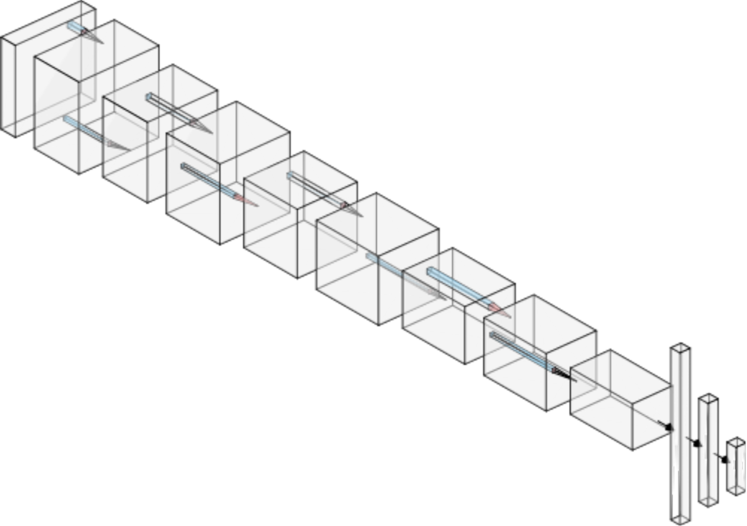
Figure 1: The 2D-CNN architecture visualized. The feature map (output) produced by each layer is the input into the next layer. Convolution and pooling layers get progressively deeper. The height and width of the feature maps become smaller through pooling.

The rectified linear unit (ReLU) is a non-linear activation function used on many of the layers in the network and is defined as

$$f(x)=\max(0,x).$$ (3)

The softmax function is used as the final activation, the output of which is an 18-dimensional vector of probabilities for each image/sequence. This is defined as

$$\hat{p}_{i}^{(c)}=\frac{\exp(w_{c}^{T}x)}{\sum_{c=1}^{C}\exp(w_{c}^{T}x)},\quad c=1,2,\ldots,C,$$ (4)

where $x$ is the feature map from the previous layer, $w_{c}$ is the vector of weights connecting the output from the previous layer to class $c$, $C=18$ as we have 18 different EOS we are classifying, and $(\hat{p}_{i}^{(1)},\hat{p}_{i}^{(2)},\ldots,\hat{p}_{i}^{(C)})$ is the vector of probabilities for the $i^{\mathrm{th}}$ image/sequence.

The loss function that we minimize is the categorical cross-entropy, which is commonly-used throughout multi-class classification problems. This is defined as

$$L(p,\hat{p})=-\sum_{i=1}^{N}\sum_{c=1}^{C}p_{i}^{(c)}\log\hat{p}_{i}^{(c)},$$ (5)

where $N$ is the number of images/sequences in the training set and

$$p_{i}^{(c)}=\begin{cases}1&\text{if image/sequence $i$ belongs to class $c$},\\ 0&\text{otherwise}.\end{cases}$$ (6)

We use the RMSProp optimizer as our gradient descent routine. The CNN is implemented in Python using the Keras deep learning framework (Chollet, 2018).

III Preprocessing

We use the 1824 simulated rotating core collapse GW signals of Richers et al (2017), and the data is publicly available at (Richers et al, 2016).

Each signal in the data set has a source distance of 10 kpc from Earth. The data is originally sampled at 65535 Hz. We downsample the data to 4096 Hz, limiting the analysis to the most sensitive part of the Advanced LIGO/Virgo frequency band as these ground-based GW detectors will not be sensitive to high frequencies in the core collapse signal due to photon shot noise.

Before downsampling, we first multiply the time-domain data by a Tukey window with tapering parameter $\alpha=0.1$ to mitigate spectral leakage, and apply a low-pass Butterworth filter (with order 10 and attenuation 0.25) to prevent aliasing. We then downsample by removing data according to the linear interpolation digital resampling algorithm outlined by Smith and Gossett (1984).

We align all signals such that $t_{b}=0$, where $t_{b}$ is the time of core bounce, and restrict our attention to the signal at times $t\in[t_{b}-0.05~{}\text{s},t_{b}+0.075~{}\text{s}]$, as this is where the most interesting dynamics of the GW signal occur. This is the direct sequence input for the 1D-CNN, but further processing is required for the 2D-CNNs.

No noise (simulated or real) is added to the signal in this paper as our primary goal is to explore the GW signal dependence on the nuclear EOS.

We need to produce the images to feed into the 2D-CNN. We explore the data in three different ways; in the time-domain with the time series signal, in the frequency-domain with the periodogram (squared modulus of Fourier coefficients), and in time-frequency space with a spectrogram.

First, we create images of the time-domain data. We transform the data set so all signals are on the unit interval. We translate all signals by subtracting the minimum strain from across the entire catalogue, and then rescale by dividing by the maximum strain from across the entire catalogue. We plot the data, making sure to remove the axes, scales, ticks, and labels, as these will add unwanted noise in the image. We then save each image as a (256 $\times$ 256) pixel image in jpeg format. An example of one of these time series images is illustrated in Figure 2.

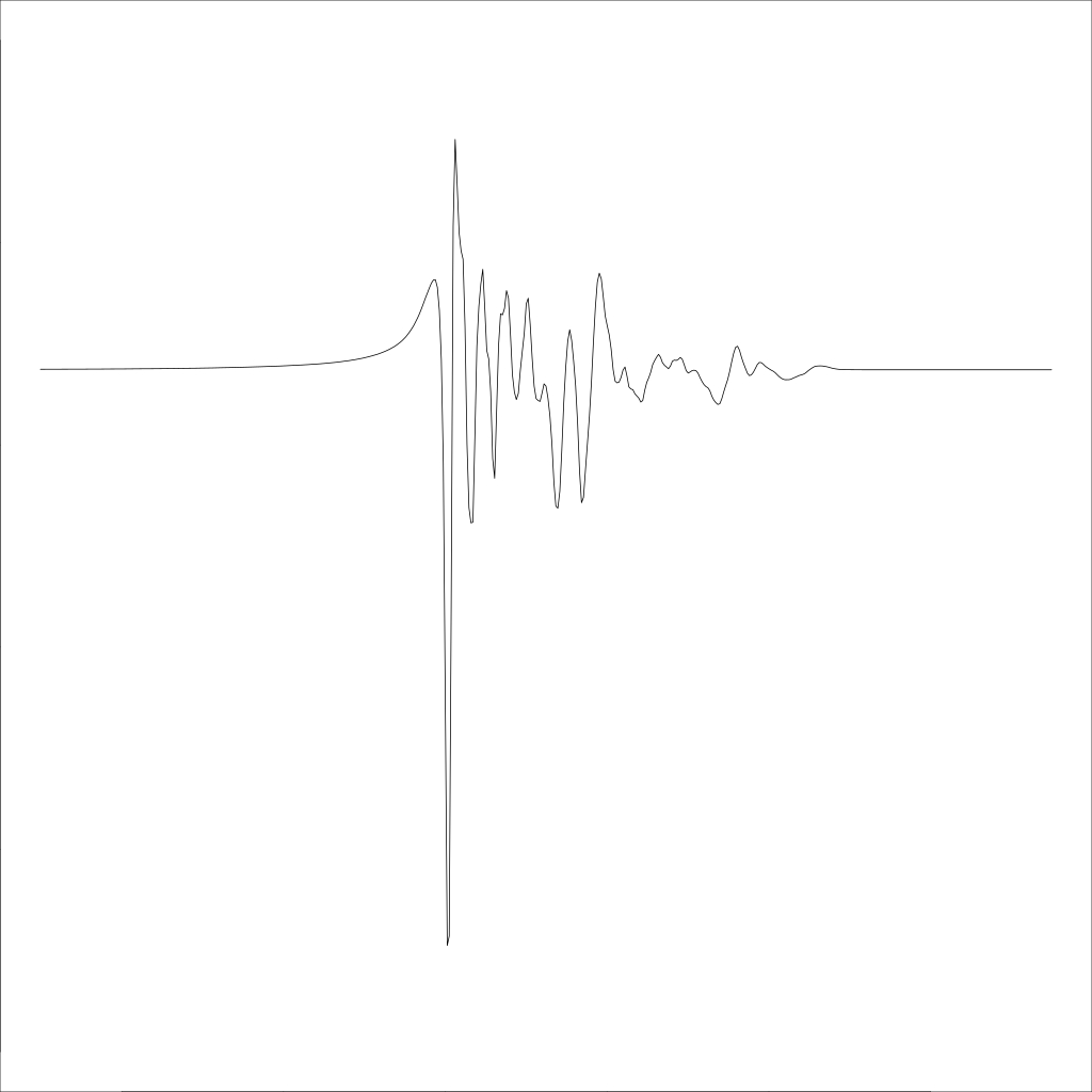
Figure 2: 256 $\times$ 256 pixel image of the time series of the 670th signal in the Richers et al (2017) catalogue. This signal comes from a $12~{}M_{\odot}$ progenitor, using the HShen EOS, with differential rotation of $A=30~{}\mathrm{km}$, and maximum initial rotation rate of $\Omega_{0}=11~{}\mathrm{rad~{}s^{-1}}$.

The second set of images are the periodograms of the GW signals. The squared modulus of the Fourier coefficients is computed and then transformed to the unit interval by translating and rescaling as before (using the minimum/maximum power from the entire catalogue). The resulting frequency-domain representations are plotted (on the $\log_{10}$ scale) and saved in jpeg format as before. The periodogram of the signal presented in Figure 2 is displayed in Figure 3.

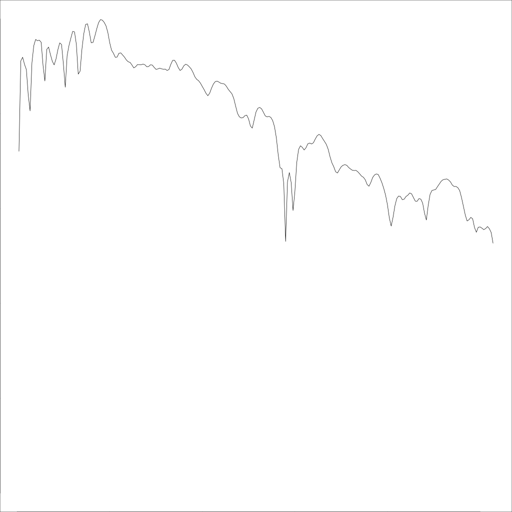
Figure 3: 256 $\times$ 256 pixel image of the periodogram of the 670th signal in the Richers et al (2017) catalogue. This signal comes from a $12~{}M_{\odot}$ progenitor, using the HShen EOS, with differential rotation of $A=30~{}\mathrm{km}$, and maximum initial rotation rate of $\Omega_{0}=11~{}\mathrm{rad~{}s^{-1}}$.

The third set of images are time-frequency maps of the data. We generate the ($256\times 256$ pixel jpeg) images by computing and plotting the spectrogram, which represents a signal’s power content over time and frequency. We use a window length of $2^{7}$, an overlap of 99%, and Tukey tapering parameter $\alpha=0.01$.

An example image used as input into the algorithm is presented in Figure 4. Note that the frequency axis is on the $\log_{2}$ scale, and power (colour) is normalized by dividing the power in each of the spectrograms by the maximum total power from across the entire catalogue to ensure images are all on the same scale. As before, axes, ticks, scales, and labels are removed.

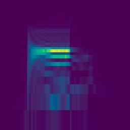
Figure 4: 256 $\times$ 256 image of the spectrogram of the 670th signal in the Richers et al (2017) catalogue. This signal comes from a $12~{}M_{\odot}$ progenitor, using the HShen EOS, with differential rotation of $A=30~{}\mathrm{km}$, and maximum initial rotation rate of $\Omega_{0}=11~{}\mathrm{rad~{}s^{-1}}$.

For each of the three image data sets and the one sequence data set, we then randomly shuffle the images/sequences such that $\sim 70\%$ are in the training set ($n_{\mathrm{training}}=1302$), $\sim 15\%$ are in the validation set ($n_{\mathrm{validation}}=261$), and $\sim 15\%$ are in the test set ($n_{\mathrm{test}}=261$).

We run three separate 2D-CNNs (one each for the time series images, periodogram images, and spectrogram images) to explore visual patterns, and one 1D-CNN on the sequence data to explore temporal patterns, with the goal of classifying nuclear EOS.

The input depth for the time series and periodogram images is one grayscale colour channel, whereas for the spectrogram images, this is a three colour RGB channel. The input depth for the sequence data is one as we only have univariate time series data.

IV Results

We measure the success of the four CNNs in terms of the proportion of test signals that have the correct EOS classification, called the accuracy of the network. In this study, we achieve 64% accuracy for the spectrogram images, 65% for the periodogram images, 71% for the time series images, and 72% for the direct sequence data.

State-of-the-art CNNs can achieve accuracies of up to 95-99% on every-day objects in computer vision competitions such as those based on the ImageNet database (Russakovsky et al, 2015). This has been demonstrated effectively in the GW literature (see e.g., (George et al, 2018)). Though our achieved accuracy of 64–72% is lower than this, it is much higher than anticipated. As noted by Richers et al (2017), the rotating core collapse GW signal has only very weak dependence on nuclear EOS. Our results suggest that this could be upgraded to “moderate” dependence. What is also surprising is the algorithm achieved this accuracy with a relatively small training data set ($n=1302$).

Let us now consider the “top 5” EOS classifications for each image/sequence. That is, the five EOS classes with the highest probabilities for each image/sequence. We compute the cumulative proportion of images/sequences in the test set that are correctly classified within these top 5 classes. The cumulative proportion of correct classifications can be seen in Table 2. Interestingly, the 2D-CNN trained on time series images outperforms the other 2D-CNNs, and the 1D-CNN does slightly better than this. For each CNN, the EOS class with the second highest probability is the correct classification on more than 10% of the test signals, indicating that we can correctly classify the EOS within the top 2 classes 75–88% of the time. For the 1D-CNN and the time series 2D-CNN, we achieve more than 90% correct classifications within the top 3 EOS classes. We can can correctly constrain the nuclear EOS to one in five classes (rather than one in 18) 97%, 93%, 91%, and 97% of the time for the time series 2D-CNN, periodogram 2D-CNN, spectrogram 2D-CNN, and sequence 1D-CNN respectively. These results are encouraging and demonstrate that we can constrain the nuclear EOS with reasonable accuracy. It is worth noting for the spectrogram images that a 2D-CNN with one grayscale input colour channel yields consistent results to the 2D-CNN with three RGB input colour channels presented here. However, these results have been omitted for brevity.

Table 2: Cumulative proportion of correct classifications.

	2D-CNN			1D-CNN
	Time Series	Periodogram	Spectrogram	Sequence
1	0.71	0.65	0.64	0.72
2	0.85	0.77	0.75	0.88
3	0.91	0.85	0.83	0.91
4	0.93	0.90	0.85	0.94
5	0.97	0.93	0.91	0.97

Although Iess et al (2020) found that their 2D-CNN on spectrogram images slightly outperformed their 1D-CNN on sequence data (due to common features in the spectrograms), we find the opposite here. The raw GW sequences are the purest form of the data. This is particularly true when no noise is added to the signal, as assumed here. Converting time series to images requires further preprocessing with certain user decisions to be made. This could create image-induced uncertainty, which could have an effect on the predictive power of the 2D-CNNs. For example, spectrogram images are subject to choices in window type, window length, and overlap percentage, as well as plotting decisions such as image resolution, and results could depend on these choices. Therefore, the superior accuracy of the 1D-CNN is not surprising in the present work.

We ran the CNNs in batches of size 32 for 100 epochs for the 2D-CNNs and 30 epochs for the 1D-CNN, making sure to monitor validation accuracy and loss. Overfitting was not an issue with the 2D-CNNs, even though it is a relatively small data set. No regularization, drop-out, or $K$-fold validation was required. While training accuracy tended towards 100% as the number of epochs increased, validation accuracy remained reasonably constant at 60–70% after about 40 epochs for the 2D-CNNs, and this translated to the test set. Validation loss did not noticeably increase as the epochs increased. The 1D-CNN required fewer epochs and started noticeably overfitting after about 30 epochs.

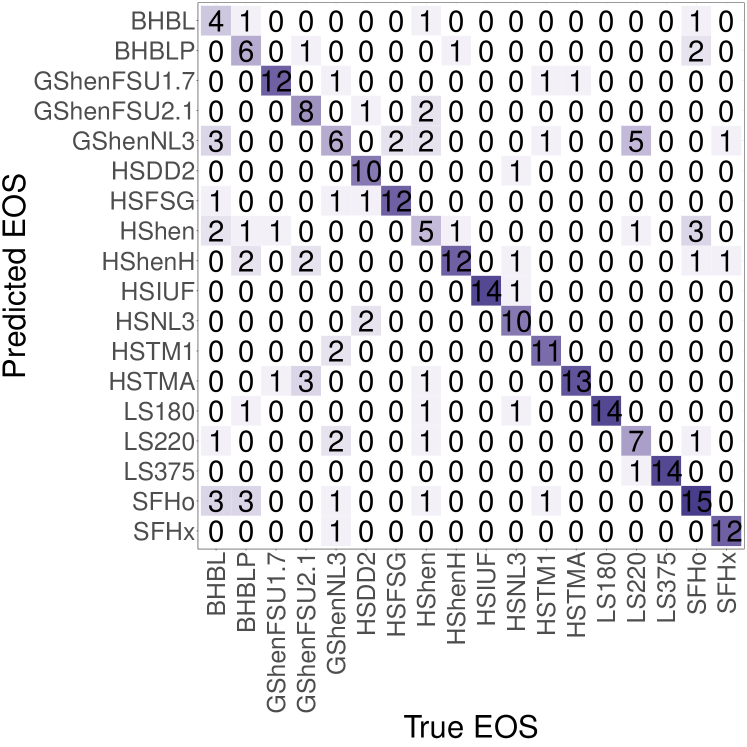
Figure 5: Confusion matrix for the test set of time series images. The darker the colour, the higher the number of correct classifications.

In Figure 5, we produce a confusion matrix that compares the true EOS class against the predicted EOS class for the test set of time series images. The confusion matrix gives us information on which EOS classes are well-classified, and which ones the CNN struggles to classify. For example, we can see that the CNN can classify the GShenFSU1.7, HSDD2, HSFSG, HShenH, HSIUF, HSNL3, HSTM1, HSTMA, LS180, LS375, and SFHx EOS with very good accuracy (at least 10 out of 14 signals), and SFHo with moderate accuracy of 15 out of 23 signals. We also see that the BHBL and HShen EOS are relatively poorly classified, noting that the BHBL EOS is often confused as the GShenNL3, HShen, and SFHo EOS, and the HShen EOS confusion is spread amongst many different EOS.

As discussed by Richers et al (2017), the EOS that are in best agreement with experimental and astrophysical constraints are LS220, GShenFSU2.1, HSDD2, SFHo, SFHx, and BHBLP. From the confusion matrix, we see that of these more astrophysically realistic EOS, HSDD2, SFHo, and SFHx are classified well, with little confusion. However, the other three astrophysically realistic EOS classes are misclassified $\sim 50\%$ of the time. Of note, the LS220 EOS is misclassified as the GShenNL3 EOS for 5 out of the 14 test signals in that class. We can also see that the BHBLP EOS often gets confused with the SFHo and HShenH EOS, and the GShenFSU2.1 EOS is often confused with the HSTMA and HShenH EOS.

V Conclusions

This paper demonstrated a proof-of-concept that rotating core collapse GW signals moderately depend on the nuclear EOS. We are encouraged by the 64–72% correct classifications achieved when using the CNN framework to probe visual and temporal patterns in rotating core collapse GW signals. We are further encouraged by the 91–97% correct classifications after considering the five EOS classes with the highest estimated probability for each test signal. With this in mind, we plan a follow-up study to explore further how the feature maps of each layer can help understand exactly how each nuclear EOS influences the GW signal.

The goal of this paper was not to conduct parameter estimation in the presence of noise, but more to explore the dependence a rotating core collapse GW signal has on the nuclear EOS. However, this is a goal of a future project, where we aim to add real or simulated detector noise to see if we can constrain nuclear EOS under more realistic settings.

The deep learning framework is becoming a force of its own in the GW data analysis literature; allowing for near-instantaneous low-latency Bayesian posterior computations using pre-trained networks, producing accurate and efficient GW signal and glitch classifications, and allowing us to solve problems previously thought impossible.

References

- Aasi et al (2015) Aasi J, et al (2015) Advanced LIGO. Classical and Quantum Gravity 32(7):074,001, DOI 10.1088/0264-9381/32/7/074001, URL https://doi.org/10.1088%2F0264-9381%2F32%2F7%2F074001
- Abbott et al (2020) Abbott B, et al (2020) Optically targeted search for gravitational waves emitted by core-collapse supernovae during the first and second observing runs of Advanced LIGO and Advanced Virgo. Phys Rev D 101:084,002, DOI 10.1103/PhysRevD.101.084002, URL https://link.aps.org/doi/10.1103/PhysRevD.101.084002
- Abdikamalov et al (2014) Abdikamalov E, Gossan S, DeMaio AM, Ott CD (2014) Measuring the angular momentum distribution in core-collapse supernova progenitors with gravitational waves. Physical Review D 90:044,001
- Acernese et al (2014) Acernese F, et al (2014) Advanced Virgo: a second-generation interferometric gravitational wave detector. Classical and Quantum Gravity 32(2):024,001, DOI 10.1088/0264-9381/32/2/024001, URL https://doi.org/10.1088%2F0264-9381%2F32%2F2%2F024001
- Astone et al (2018) Astone P, Cerdá-Durán P, Di Palma I, Drago M, Muciaccia F, Palomba C, Ricci F (2018) New method to observe gravitational waves emitted by core collapse supernovae. Phys Rev D 98:122,002, DOI 10.1103/PhysRevD.98.122002, URL https://link.aps.org/doi/10.1103/PhysRevD.98.122002
- Chan et al (2019) Chan ML, Heng I, Messenger C (2019) Detection and classification of supernova gravitational waves signals: A deep learning approach. arXivorg URL http://search.proquest.com/docview/2331700621/
- Chollet (2018) Chollet F (2018) Deep Learning with Python. Manning Publications Co., Shelter Island, New York
- Chua and Vallisneri (2020) Chua AJK, Vallisneri M (2020) Learning Bayesian posteriors with neural networks for gravitational-wave inference. Phys Rev Lett 124:041,102, DOI 10.1103/PhysRevLett.124.041102, URL https://link.aps.org/doi/10.1103/PhysRevLett.124.041102
- Dimmelmeier et al (2008) Dimmelmeier H, Ott CD, Marek A, Janka HT (2008) The gravitational wave burst signal from core collapse of rotating stars. Physical Review D 78:064,056
- Dreissigacker et al (2019) Dreissigacker C, Sharma R, Messenger C, Zhao R, Prix R (2019) Deep-learning continuous gravitational waves. Phys Rev D 100:044,009, DOI 10.1103/PhysRevD.100.044009, URL https://link.aps.org/doi/10.1103/PhysRevD.100.044009
- Edwards et al (2014) Edwards MC, Meyer R, Christensen N (2014) Bayesian parameter estimation of core collapse supernovae using gravitational wave simulations. Inverse Problems 30(11), DOI 10.1088/0266-5611/30/11/114008
- Gabbard et al (2018) Gabbard H, Williams M, Hayes F, Messenger C (2018) Matching matched filtering with deep networks for gravitational-wave astronomy. Phys Rev Lett 120:141,103, DOI 10.1103/PhysRevLett.120.141103, URL https://link.aps.org/doi/10.1103/PhysRevLett.120.141103
- Gabbard et al (2019) Gabbard H, Messenger C, Heng IS, Tonolini F, Murray-Smith R (2019) Bayesian parameter estimation using conditional variational autoencoders for gravitational-wave astronomy. arXiv:190906296 [astro-phIM]
- George and Huerta (2018) George D, Huerta E (2018) Deep learning for real-time gravitational wave detection and parameter estimation: Results with Advanced LIGO data. Physics Letters B 778:64 – 70, DOI https://doi.org/10.1016/j.physletb.2017.12.053, URL http://www.sciencedirect.com/science/article/pii/S0370269317310390
- George et al (2018) George D, Shen H, Huerta EA (2018) Classification and unsupervised clustering of LIGO data with deep transfer learning. Phys Rev D 97:101,501, DOI 10.1103/PhysRevD.97.101501, URL https://link.aps.org/doi/10.1103/PhysRevD.97.101501
- Goodfellow et al (2016) Goodfellow I, Bengio Y, Courville A (2016) Deep Learning. The MIT Press
- Gossan et al (2016) Gossan SE, Sutton P, Stuver A, Zanolin M, Gill K, Ott CD (2016) Observing gravitational waves from core-collapse supernovae in the advanced detector era. Phys Rev D 93:042,002, DOI 10.1103/PhysRevD.93.042002, URL https://link.aps.org/doi/10.1103/PhysRevD.93.042002
- Green and Gair (2020) Green SR, Gair J (2020) Complete parameter inference for gw150914 using deep learning. arXiv:200803312 [astro-phIM]
- Green et al (2020) Green SR, Simpson C, Gair J (2020) Gravitational-wave parameter estimation with autoregressive neural network flows. arXiv:200207656 [astro-phIM]
- Iess et al (2020) Iess A, Cuoco E, Morawski F, Powell J (2020) Core-collapse supernova gravitational-wave search and deep learning classification. Machine Learning: Science and Technology 1(2):025,014, DOI 10.1088/2632-2153/ab7d31, URL https://doi.org/10.1088%2F2632-2153%2Fab7d31
- Janka (2012) Janka HT (2012) Explosion mechanisms of core-collapse supernovae. Annual Review of Nuclear and Particle Science 62(1):407–451, DOI 10.1146/annurev-nucl-102711-094901, URL https://doi.org/10.1146/annurev-nucl-102711-094901, eprint https://doi.org/10.1146/annurev-nucl-102711-094901
- Kuroda et al (2017) Kuroda T, Kotake K, Hayama K, Takiwaki T (2017) Correlated signatures of gravitational-wave and neutrino emission in three-dimensional general-relativistic core-collapse supernova simulations. The Astrophysical Journal 851(1):62, DOI 10.3847/1538-4357/aa988d, URL https://doi.org/10.3847%2F1538-4357%2Faa988d
- Lattimer (2012) Lattimer JM (2012) The nuclear equation of state and neutron star masses. Annual Review of Nuclear and Particle Science 62(1):485–515, DOI 10.1146/annurev-nucl-102711-095018, URL https://doi.org/10.1146/annurev-nucl-102711-095018, eprint https://doi.org/10.1146/annurev-nucl-102711-095018
- Logue et al (2012) Logue J, Ott CD, Heng I, Kalmus P, Scargill JHC (2012) Inferring core-collapse supernova physics with gravitational waves. Phys Rev D 86:044,023, DOI 10.1103/PhysRevD.86.044023, URL https://link.aps.org/doi/10.1103/PhysRevD.86.044023
- MacKay (2003) MacKay DJC (2003) Information Theory, Inference, and Learning Algorithms. Cambridge University Press, USA
- Powell et al (2016) Powell J, Gossan SE, Logue J, Heng IS (2016) Inferring the core-collapse supernova explosion mechanism with gravitational waves. Phys Rev D 94:123,012, DOI 10.1103/PhysRevD.94.123012, URL https://link.aps.org/doi/10.1103/PhysRevD.94.123012
- Powell et al (2017) Powell J, Szczepanczyk M, Heng IS (2017) Inferring the core-collapse supernova explosion mechanism with three-dimensional gravitational-wave simulations. Phys Rev D 96:123,013, DOI 10.1103/PhysRevD.96.123013, URL https://link.aps.org/doi/10.1103/PhysRevD.96.123013
- Richers et al (2016) Richers S, Ott CD, Abdikamalov E, O’Connor E, Sullivan C (2016) Equation of State Effects on Gravitational Waves from Rotating Core Collapse. DOI 10.5281/zenodo.201145, URL https://doi.org/10.5281/zenodo.201145
- Richers et al (2017) Richers S, Ott CD, Abdikamalov E, O’Connor E, Sullivan C (2017) Equation of state effects on gravitational waves from rotating core collapse. Phys Rev D 95:063,019, DOI 10.1103/PhysRevD.95.063019, URL https://link.aps.org/doi/10.1103/PhysRevD.95.063019
- Röver et al (2009) Röver C, Bizouard MA, Christensen N, Dimmelmeier H, Heng I, Meyer R (2009) Bayesian reconstruction of gravitational wave burst signals from simulations of rotating stellar core collapse and bounce. Physical Review D - Particles, Fields, Gravitation and Cosmology 80(10), DOI 10.1103/PhysRevD.80.102004
- Russakovsky et al (2015) Russakovsky O, Deng J, Su H, Krause J, Satheesh S, Ma S, Huang Z, Karpathy A, Khosla A, Bernstein M, Berg AC, Fei-Fei L (2015) ImageNet Large Scale Visual Recognition Challenge. International Journal of Computer Vision (IJCV) 115(3):211–252, DOI 10.1007/s11263-015-0816-y
- Shen et al (2019) Shen H, Huerta EA, Zhao Z, Jennings E, Sharma H (2019) Deterministic and Bayesian neural networks for low-latency gravitational wave parameter estimation of binary black hole mergers. arXiv:190301998 [gr-qc]
- Smith and Gossett (1984) Smith J, Gossett P (1984) A flexible sampling-rate conversion method. In: ICASSP ’84. IEEE International Conference on Acoustics, Speech, and Signal Processing, vol 9, pp 112–115
- Somiya (2012) Somiya K (2012) Detector configuration of KAGRA–the japanese cryogenic gravitational-wave detector. Classical and Quantum Gravity 29(12):124,007, DOI 10.1088/0264-9381/29/12/124007, URL https://doi.org/10.1088%2F0264-9381%2F29%2F12%2F124007
- Zevin et al (2017) Zevin M, Coughlin S, Bahaadini S, Besler E, Rohani N, Allen S, Cabero M, Crowston K, Katsaggelos AK, Larson SL, Lee TK, Lintott C, Littenberg TB, Lundgren A, Østerlund C, Smith JR, Trouille L, Kalogera V (2017) Gravity Spy: integrating Advanced LIGO detector characterization, machine learning, and citizen science. Classical and Quantum Gravity 34(6):064,003, DOI 10.1088/1361-6382/aa5cea, URL https://doi.org/10.1088%2F1361-6382%2Faa5cea