Fast semantic parsing with well-typedness guarantees

Abstract

AM dependency parsing is a linguistically principled method for neural semantic parsing with high accuracy across multiple graphbanks. It relies on a type system that models semantic valency but makes existing parsers slow. We describe an A* parser and a transition-based parser for AM dependency parsing which guarantee well-typedness and improve parsing speed by up to 3 orders of magnitude, while maintaining or improving accuracy.

1 Introduction

Over the past few years, the accuracy of neural semantic parsers which parse English sentences into graph-based semantic representations has increased substantially Dozat and Manning (2018); Zhang et al. (2019); He and Choi (2020); Cai and Lam (2020). Most of these parsers use a neural model which can freely predict node labels and edges, and most of them are tailored to a specific type of graphbank.

Among the high-accuracy semantic parsers, the AM dependency parser of Groschwitz et al. (2018) stands out in that it implements the Principle of Compositionality from theoretical semantics in a neural framework. By parsing into AM dependency trees, which represent the compositional structure of the sentence and evaluate deterministically into graphs, this parser can abstract away surface details of the individual graphbanks. It was the first semantic parser which worked well across multiple graphbanks, and set new states of the art on several of them Lindemann et al. (2019).

However, the commitment to linguistic principles comes at a cost: the AM dependency parser is slow. A key part of the parser is that AM dependency trees must be well-typed according to a type system which ensures that the semantic valency of each word is respected. Existing algorithms compute all items along a parsing schema that encodes the type constraints; they parse e.g. the AMRBank at less than three tokens per second.

In this paper, we present two fast and accurate parsing algorithms for AM dependency trees. We first present an A* parser which searches through the parsing schema of Groschwitz et al.’s “projective parser” efficiently (§4). We extend the supertag-factored heuristic of Lewis and Steedman’s Lewis and Steedman (2014) A* parser for CCG with a heuristic for dependency edge scores. This parser achieves a speed of up to 2200 tokens/s on semantic dependency parsing Oepen et al. (2015), at no loss in accuracy. On AMR corpora Banarescu et al. (2013), it achieves a speedup of 10x over previous work, but still does not exceed 30 tokens/second.

We therefore develop an entirely new transition-based parser for AM dependency trees, inspired by the stack-pointer parser of Ma et al. (2018) for syntactic dependency parsing (§5). The key challenge here is to adhere to complex symbolic constraints – the AM algebra’s type system – without running into dead ends. This is hard for a greedy transition system and in other settings requires expensive workarounds, such as backtracking. We ensure that our parser avoids dead ends altogether. We define two variants of the transition-based parser, which choose types for words either before predicting the outgoing edges or after, and introduce a neural model for predicting transitions. In this way, we guarantee well-typedness with $O(n^{2})$ parsing complexity, achieve a speed of several thousand tokens per second across all graphbanks, and even improve the parsing accuracy over previous AM dependency parsers by up to 1.6 points F-score.

2 Related work

In transition-based parsing, a dependency tree is built step by step using nondeterministic transitions. A classifier is trained to choose transitions deterministically Nivre (2008); Kiperwasser and Goldberg (2016). Transition-based parsing has also been used for constituency parsing (Dyer et al., 2016) and graph parsing Damonte et al. (2017). We build most directly upon the top-down parser of Ma et al. (2018). Unlike most other transition-based parsers, our parser implements hard symbolic constraints in order to enforce well-typedness. Such constraints can lead transition systems into dead ends, requiring the parser to backtrack (Ytrestøl, 2011) or return partial analyses (Zhang and Clark, 2011). Our transition system carefully avoids dead ends. Shi and Lee (2018) take hard valency constraints into account in chart-based syntactic dependency parsing, avoiding dead ends by relaxing the constraints slightly in practice.

A* parsing is a method for speeding up agenda-based chart parsers, which takes items off the agenda based on a heuristic estimate of completion cost. A* parsing has been used successfully for PCFGs Klein and Manning (2003), TAG Bladier et al. (2019), and other grammar formalisms. Our work is based most closely on the CCG A* parser of Lewis and Steedman (2014).

Most approaches that produce semantic graphs (see Koller et al. (2019) for an overview) model distributions over graphs directly (Dozat and Manning, 2018; Zhang et al., 2019; He and Choi, 2020; Cai and Lam, 2020), while others make use of derivation trees that compositionally evaluate to graphs (Groschwitz et al., 2018; Chen et al., 2018; Fancellu et al., 2019; Lindemann et al., 2019). AM dependency parsing belongs to the latter category.

3 Background

We begin by sketching the AM dependency parser of Groschwitz et al. (2018).

3.1 AM dependency trees

Groschwitz et al. (2018) use AM dependency trees to represent the compositional structure of a semantic graph. Each token is assigned a graph constant representing its lexical meaning; dependency labels correspond to operations of the Apply-Modify (AM) algebra (Groschwitz et al., 2017; Groschwitz, 2019), which combine graphs into bigger ones.

Fig. 2 illustrates how an AM dependency tree (a) evaluates to a graph (b), based on the graph constants in Fig. 1. Each graph constant is an as-graph, which means it has special node markers called sources, drawn in red, as well as a root marked in bold. These markers are used to combine graphs with the algebra’s operations. For instance, the mod${}_{\text{{M}}}$ operation in Fig. 2a combines the head $G_{\text{sleep}}$ with its modifier $G_{\text{soundly}}$ by plugging the root of $G_{\text{sleep}}$ into the M-source of $G_{\text{soundly}}$, see (c). That is, $G_{\text{soundly}}$ has now modified $G_{\text{sleep}}$ and (c) is our graph for sleep soundly. The other operation of the AM algebra, App, models argument application. For example, the App${}_{\text{{O}}}$ operation in Fig. 2a plugs the root of (c) into the O source of $G_{\text{want}}$. Note that because $G_{\text{want}}$ and (c) both have an S-source, App${}_{\text{{O}}}$ merges these nodes, see (d). The App${}_{\text{{S}}}$ operation then fills this S-source with $G_{\text{writer}}$, attaching the graph with its root, to obtain the final graph in (b).

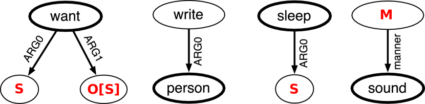
Figure 1: Elementary as-graphs $G_{\text{want}}$, $G_{\text{writer}}$, $G_{\text{sleep}}$, and $G_{\text{sound}}$.

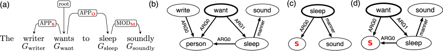
Figure 2: (a) An AM dependency tree with its evaluation result (b), along with two partial results (c) and (d).

Types. The $[\text{{S}}]$ annotation at the O-source of $G_{\text{want}}$ is a request as to what the type of the O argument of $G_{\text{want}}$ should be. The type of an as-graph is the set of its sources with their request annotations, so the request $[\text{{S}}]$ means that the source set of the argument must be $\{\text{{S}}\}$. Because this is true for (c), the AM dependency tree is well-typed; otherwise the tree could not be evaluated to a graph. Thus, the graph constants lexically specify the semantic valency of each word as well as reentrancies due to e.g. control, like in this example.

If an as-graph has no sources, we say it has the empty type $[\,]$; if a source in a graph printed here has no annotation, it is assumed to have the empty request (i.e. its argument must have no sources). We write $\tau_{G}$ for the type of an as-graph $G$, and $\text{{req}}_{\alpha}(\tau)$ for the request at source $\alpha$ of type $\tau$. For example, $\text{{req}}_{\text{{O}}}($$\tau_{G_{\text{want}}}$$)=[\text{{S}}]$ and $\text{{req}}_{\text{{S}}}($$\tau_{G_{\text{want}}}$$)=[\,]$. If an AM dependency (sub-)tree evaluates to a graph $G$, we call $\tau_{G}$ its term type. For example, the sub-tree in Fig. 2a rooted in sleep has term type $[\text{{S}}]$, since it evaluates to (c).

Below, we will build AM dependency trees by adding the outgoing edges of a node one by one; we track types there with the following notation. If $\tau_{1}$ and $\tau_{2}$ are the term types of AM dependency trees $t_{1},t_{2}$ and $\ell$ is an operation of the AM algebra, we write $\ell\left(\tau_{1},\tau_{2}\right)$ for the term type of the tree constructed by adding $t_{2}$ as an $\ell$-child to $t_{1}$, i.e. by adding an $\ell$-edge from the root of $t_{1}$ to the root of $t_{2}$ (if that tree is well-typed). Intuitively, one can see this as combining a graph of type $\tau_{1}$ (the head) with an argument or modifier of type $\tau_{2}$ using operation $\ell$; the result then has type $\ell\left(\tau_{1},\tau_{2}\right)$.

3.2 AM dependency parsing

Groschwitz et al. (2018) approach graph parsing as first predicting a well-typed AM dependency tree for a sentence $w_{1},\dots,w_{n}$ and then evaluating it deterministically to obtain the graph.

They train a supertag and edge-factored model, which predicts a supertag cost $c\left(G,i\right)$ for assigning a graph constant $G$ to the token $w_{i}$, as well as an edge cost $c\left(i\xrightarrow{\text{$\ell$}}j\right)$ for each potential edge from word $w_{i}$ to $w_{j}$ with label $\ell$. Tokens which are not part of the AM dependency tree, like the and to in Fig. 2a, are treated as if they were assigned the special graph constant $\bot$ and an incoming ‘ignore’ edge $0\xrightarrow{\text{\text{{ignore}}}}i$, where $0$ represents an artificial root. The root of the AM dependency tree (wants in the example) is modeled as having an incoming edge $0\xrightarrow{\text{{root}}}i$.

An algorithm for AM dependency parsing searches for the well-typed AM dependency tree which minimizes the sum of supertag and edge costs. Finding the lowest-cost well-typed AM dependency tree for a given sentence is NP-complete. Groschwitz et al. define two approximate parsing algorithms, the ‘fixed tree decoder’ that fixes an unlabeled dependency tree first , and the ‘projective decoder’. Our A* parser is based on the projective decoder and we focus on it here.

Projective decoder. The projective decoder circumvents the NP-completeness by searching for the best projective well-typed AM dependency tree. It derives parsing items using the schema (Shieber et al., 1995) shown in Fig. 3.

Each item encodes properties of a partial AM dependency tree and has the form $([i,k],r,\tau):s$, where $[i,k]=\{j\mid i\leq j<k\}$ is the span of word indices covered by the item, $r$ is the index of the head word, $\tau$ the type and $s$ the cost. The Init rule assigns a supertag $G$ to a word $w_{i}$. The Skip-R and Skip-L rules extend a span without changing the dependency derivation, effectively skipping a word by assigning it the $\bot$ supertag and drawing the corresponding ‘ignore’ edge. Finally the Arc-R and Arc-L rules, for an AM operation $\ell$, combine two items covering adjacent spans by drawing an edge with label $\ell$ between their heads. Once the full chart is computed, i.e. all items are explored, a Viterbi algorithm yields the highest scoring well-typed AM dependency tree.

The projective decoder has an asymptotic runtime of $O\left(n^{5}\right)$ in the sentence length $n$.

$\displaystyle\begin{array}[]{@{}c@{}}s=c\left(G,i\right)\quad G\neq\bot\\ \hline\cr([i,i+1],i,\tau_{G}):s\end{array}$   Init
$\displaystyle\begin{array}[]{@{}c@{}}([i,k],r,\tau):s\quad s^{\prime}=c\left(\bot,k\right)+c\left(0\xrightarrow{\text{\text{{ignore}}}}k\right)\\ \hline\cr([i,k+1],r,\tau):s+s^{\prime}\end{array}$   Skip-R
$([i,k],r,\tau):s$ $s^{\prime}=c\left(\bot,i-1\right)+c\left(0\xrightarrow{\text{\text{{ignore}}}}i-1\right)$  Skip-L                     $([i-1,k],r,\tau):s+s^{\prime}$
$([i,j],r_{1},\tau_{1}):s_{1}\quad([j,k],r_{2},\tau_{2}):s_{2}$ $\tau=\ell(\tau_{1},\tau_{2})\;\mbox{defined}\quad s=c\left(r_{1}\xrightarrow{\text{$\ell$}}r_{2}\right)$  Arc-R [$\ell$]                                   $([i,k],r_{1},\tau):s_{1}+s_{2}+s$
$([i,j],r_{1},\tau_{1}):s_{1}\quad([j,k],r_{2},\tau_{2}):s_{2}$ $\tau=\ell(\tau_{2},\tau_{1})\;\mbox{defined}\quad s=c\left(r_{2}\xrightarrow{\text{$\ell$}}r_{1}\right)$  Arc-L [$\ell$]                                   $([i,k],r_{2},\tau):s_{1}+s_{2}+s$
$\displaystyle\begin{array}[]{@{}c@{}}([1,n+1],r,[\,]):\quad s^{\prime}=c\left(0\xrightarrow{\text{{root}}}r\right)\\ \hline\cr([0,n+1],r,[\,]):s+s^{\prime}\end{array}$   Root

Figure 3: Rules for the projective and A* decoder.

Notation and terminology. Below, we assume that we obtained three fixed non-empty finite sets in training: a set ${\Omega}$ of types; a set $C$ of graph constants (the graph lexicon) such that ${\Omega}$ is the set of types of the graphs in $C$; and a set $L$ of operations, including root and ignore. We write $S$ for the set of sources occurring in $C$ and assume that for every source $s\in S$, $\text{{App}}_{s}\in L$. We write $Dom(f)$ for the domain of a partial function $f$, i.e. the set of objects for which $f$ is defined.

4 A* AM dependency parsing

While the AM dependency parser yields strong accuracies across multiple graphbanks, Groschwitz et al.’s algorithms are quite slow in practice. For instance, the projective parser needs several hours to parse each test set in §6, which seriously limits its practical applicability. In this section, we will speed the projective parser up through A* search.

4.1 Agenda-based A* parsing

Our A* parser maintains an agenda of parse items of the projective parser. The agenda is initialized with the items produced by the Init rule. Then we iterate over the agenda. In each step, we take the item $I$ from the front of the agenda and apply the rules Skip-L and Skip-R to it. We also attempt to combine $I$ with all previously discovered items, organized in a parse chart, using the Arc-L and Arc-R rules. All items thus generated are added to the agenda and the chart. Parsing ends once we either take a goal item $([0,n+1],r,[\,])$ from the agenda, or (unsucessfully) when the agenda becomes empty.

A* parsers derive their efficiency from their ability to order the items on the agenda effectively. They sort the agenda in ascending order of estimated cost $f(I)=c(I)+h(I)$, where $c$ is the cost derived for the item $I$ by the parsing rules in Fig. 3 and $h(I)$ is an outside estimate. The quantity $h(I)$ estimates the difference in cost between $I$ and the lowest-cost well-typed AM dependency tree $t$ that contains $I$. An outside heuristic is admissible if it is optimistic with respect to cost, i.e. $f(I)\leq c(t)$; in this case the parser is provably optimal, i.e. the first goal item which is dequeued from the agenda describes the lowest-cost parse tree. Tighter outside estimates lead to fewer items being taken off the agenda and thus to faster runtimes.

A first trivial, but admissible baseline lets $h(I)=0$ for all items $I$. This ignores the outside part and orders items purely on their past cost. We could obtain a better outside heuristic by following Lewis and Steedman (2014) and summing up the cost of the lowest-cost supertag for each token outside of the item, i.e.

$$h([i,k],r,\tau)=\sum_{j\not\in[i,k]}\min_{G}c(G,j).$$

This heuristic is admissible because each token will have some supertag selected (perhaps $\bot$) in a complete AM dependency tree, and its cost will be equal or higher than that of the best supertag.

4.2 Edge-based A* heuristics

Both of these outside heuristics ignore the fact that the cost of a tree consists not only of the cost for the supertags, but also of the cost for the edges.

We can obtain tighter heuristics by taking the edges into account. Observe first that the parse item determines the supertags and edges within its substring, and has designated one of the tokens as the root of the subtree it represents. For all tokens outside of the span of the item, the best parse tree will assign both a supertag to the token (potentially $\bot$) and an incoming edge (potentially with edge label root or ignore). Thus, we obtain an admissible edge-based heuristic by adding the lowest-cost incoming edge for each outside token as follows:

$$h([i,k],r,\tau)=\sum_{j\not\in[i,k]}\min_{G}c(G,j)+\min_{o\xrightarrow{\ell}j}c(o\xrightarrow{\ell}j)$$

Observe finally that the edge-based heuristic is still overly optimistic, in that it assumes that arbitrarily many nodes in the tree may have incoming root edges (when it needs to be exactly one), and that the choice of ignore and $\bot$ are independent (when a node should have an incoming ignore edge if and only if its supertag is $\bot$). We can optimize it into the ignore-aware outside heuristic by restricting the $\min$ operations so they respect these constraints.

5 Transition-based parsing

As we will see in §6, the A* parser is very efficient on the DM, PAS, and PSD corpora but still slow on EDS and AMR.

Therefore, we develop a novel transition-based algorithm for AM dependency parsing. Inspired by the syntactic dependency parser of Ma et al. (2018), it builds the dependency tree top-down, starting at the root and recursively adding outgoing edges to nodes. However, for AM dependency parsing we face an additional challenge: we must assign a type to each node and ensure that the overall AM dependency tree is well-typed.

We will first introduce some notation (§5.1), then introduce three versions of our parsing schema (§5.2-§5.4), give theoretical guarantees (§5.5) and define the neural model (§5.6).

5.1 Apply sets

The transition-based parser chooses a graph constant $G_{i}$ for each token $w_{i}$; we call its type, $\tau_{G_{i}}$, the lexical type ${\color[rgb]{1,0,0}\tau\lambda l}$ of $w_{i}$. As we add outgoing edges to $i$, each outgoing $\text{{App}}_{\alpha}$ operation consumes the $\alpha$ source of the lexical type. To produce a well-typed AM dependency tree of term type ${\color[rgb]{0,0,1}\tau\lambda t}$, the sources of outgoing App edges at $i$ must correspond to exactly the apply set $\mathcal{A}\left({\color[rgb]{1,0,0}\tau\lambda l},{\color[rgb]{0,0,1}\tau\lambda t}\right)$, which is defined as the set $O=\{o_{1},\ldots,o_{n}\}$ of sources such that

$$\text{{App}}_{o_{n}}(\dots\text{{App}}_{o_{2}}(\text{{App}}_{o_{1}}({\color[rgb]{1,0,0}\tau\lambda l},{\color[rgb]{0,0,1}\tau\lambda t}_{1}),{\color[rgb]{0,0,1}\tau\lambda t}_{2}),\dots,{\color[rgb]{0,0,1}\tau\lambda t}_{n})={\color[rgb]{0,0,1}\tau\lambda t}$$

for some types ${\color[rgb]{0,0,1}\tau\lambda t}_{1},\ldots,{\color[rgb]{0,0,1}\tau\lambda t}_{n}$. That is, the apply set $\mathcal{A}\left({\color[rgb]{1,0,0}\tau\lambda l},{\color[rgb]{0,0,1}\tau\lambda t}\right)$ is the set of sources we need to consume to turn ${\color[rgb]{1,0,0}\tau\lambda l}$ into ${\color[rgb]{0,0,1}\tau\lambda t}$.

Note that there are pairs of types for which no such set of sources exists; e.g. the apply set $\mathcal{A}([\,],[s])$ is not defined. In that case, we say that $[s]$ is not apply-reachable from $[\,]$; the term type must always be apply-reachable from the lexical type in a well-typed tree.

5.2 Lexical type first (with dead ends)

Step	$\mathbb{E}$	$\mathbb{T}$	$\mathbb{A}$	$\mathbb{G}$	$\mathbb{S}$	Transition
1	$\emptyset$	$\emptyset$	$\emptyset$	$\emptyset$	$[]$
2	$0\xrightarrow{\textsc{root}}\scalebox{0.9}{}\text{\emph{wants}}_{3}$	$\scalebox{0.9}{}\text{\emph{wants}}_{3}\mapsto\{{\color[rgb]{0,0,1}[\,]}\}$			3	Init 3
3			$\scalebox{0.9}{}\text{\emph{wants}}_{3}\mapsto\emptyset$	$\scalebox{0.9}{}\text{\emph{wants}}_{3}\mapsto G_{\text{want}}$	3	Choose $[\,]$, $\langle G_{\text{want}},[s,o[s]]\rangle$
4	$\scalebox{0.9}{}\text{\emph{wants}}_{3}\xrightarrow{\text{{App}}_{s}}\scalebox{0.9}{}\text{\emph{writer}}_{2}$	$\scalebox{0.9}{}\text{\emph{writer}}_{2}\mapsto\{{\color[rgb]{0,0,1}[\,]}\}$	$\scalebox{0.9}{}\text{\emph{wants}}_{3}\mapsto\{s\}$		3 2	Apply s, 2
5			$\scalebox{0.9}{}\text{\emph{writer}}_{2}\mapsto\emptyset$	$\scalebox{0.9}{}\text{\emph{writer}}_{2}\mapsto G_{\text{writer}}$	3 2	Choose $[\,]$, $\langle G_{\text{writer}},[\,]\rangle$
6					3	Pop
7	$\scalebox{0.9}{}\text{\emph{wants}}_{3}\xrightarrow{\text{{App}}_{o}}\scalebox{0.9}{}\text{\emph{sleep}}_{5}$	$\scalebox{0.9}{}\text{\emph{sleep}}_{5}\mapsto\{{\color[rgb]{0,0,1}[s]}\}$	$\scalebox{0.9}{}\text{\emph{wants}}_{3}\mapsto\{s,o\}$		3 5	Apply o, 5
8			$\scalebox{0.9}{}\text{\emph{sleep}}_{5}\mapsto\emptyset$	$\scalebox{0.9}{}\text{\emph{sleep}}_{5}\mapsto G_{\text{sleep}}$	3 5	Choose ${\color[rgb]{0,0,1}[s]}$, $\langle G_{\text{sleep}},[s]\rangle$
9	$\scalebox{0.9}{}\text{\emph{sleep}}_{5}\xrightarrow{\text{{mod}}_{m}}\scalebox{0.9}{}\text{\emph{soundly}}_{6}$	$\scalebox{0.9}{}\text{\emph{soundly}}_{6}\mapsto\{{\color[rgb]{0,0,1}[m]},{\color[rgb]{0,0,1}[s,m]}\}$			3 5 6	Modify m, 6
10		$\scalebox{0.9}{}\text{\emph{soundly}}_{6}\mapsto\{{\color[rgb]{0,0,1}[m]}\}$	$\scalebox{0.9}{}\text{\emph{soundly}}_{6}\mapsto\emptyset$	$\scalebox{0.9}{}\text{\emph{soundly}}_{6}\mapsto G_{\text{soundly}}$	3 5 6	Choose ${\color[rgb]{0,0,1}[m]}$, $\langle G_{\text{soundly}},[m]\rangle$
11					$[]$	3 $\times$ Pop

Figure 4: Derivation with LTF of the AM dependency tree in Fig. 2. The steps show only what changed for $\mathbb{E},\mathbb{T},\mathbb{A}$ and $\mathbb{G}$; the stack $\mathbb{S}$ is shown in full. The chosen graph constants are annotated with their lexical types.

We are now ready to define a first version of the transition system for our parser. The parser builds a dependency tree top-down and manipulates parser configurations to track parsing decisions and ensure well-typedness.

A parser configuration $\langle\mathbb{E},\mathbb{T},\mathbb{A},\mathbb{G},\mathbb{S}\rangle$ consists of four partial functions $\mathbb{E},\mathbb{T},\mathbb{A},\mathbb{G}$ that map each token $i$ to the following:

$\mathbb{E}\left(i\right)$: the labeled incoming edge of $i$, written $j\xrightarrow{\ell}i$, where $j$ is the head and $l$ the label;

$\mathbb{T}\left(i\right)$: the set of possible term types at $i$;

$\mathbb{A}\left(i\right)$: the sources of outgoing App edges at $i$, i.e. which sources of the apply set we have covered;

$\mathbb{G}\left(i\right)$: the graph constant at $i$.

These functions are partial, i.e. they may be undefined for some nodes. $\mathbb{S}$ is a stack of nodes that potentially still need children; we call the node on top of $\mathbb{S}$ the active node.

The initial configuration is $\langle\emptyset,\emptyset,\emptyset,\emptyset,\emptyset\rangle$. A goal configuration has an empty stack and for all tokens $i$, it holds either that $i$ is ignored and thus has no incoming edge, or that for some type ${\color[rgb]{0,0,1}\tau\lambda t}$ and graph $G$, $\mathbb{T}(i)=\{{\color[rgb]{0,0,1}\tau\lambda t}\}$, $\mathbb{G}(i)=G$ and $\mathbb{A}(i)=\mathcal{A}(\tau_{G},{\color[rgb]{0,0,1}\tau\lambda t})$, i.e. $\mathbb{A}(i)$ must be the apply set for the lexical type $\tau_{G}$ and the term type ${\color[rgb]{0,0,1}\tau\lambda t}$. There must be at least one token that is not ignored.

The transition rules below read as follows: everything above the line denotes preconditions on when the transition can be applied; for example, that $\mathbb{T}$ must map node $i$ to some set ${\color[rgb]{0,0,1}\tau\lambda T}$ of types. The transition rule then updates the configuration by adding what is specified below the line. An example run is shown in Fig. 4.

Init. An $\textsc{Init}(i)$ transition is always the first transition and makes $i$ the root of the tree:

$\mathbb{E}$	$\mathbb{T}$	$\mathbb{A}$	$\mathbb{G}$	$\mathbb{S}$
$\emptyset$	$\emptyset$	$\emptyset$	$\emptyset$	$\emptyset$
$0\xrightarrow{root}i$	$i\mapsto\{[\,]\}$			$i$

Fixing the term type as $[\,]$ ensures that the overall evaluation result has no unfilled sources left.

Choose. If we have not yet chosen a graph constant for the active node, we assign one with the $\textsc{Choose}({\color[rgb]{0,0,1}\tau\lambda t},G)$ transition:

$i\mapsto{\color[rgb]{0,0,1}\tau\lambda T}$		$i\notin Dom(\mathbb{G})$	$\sigma|i$
$i\mapsto\{{\color[rgb]{0,0,1}\tau\lambda t}\}$	$i\mapsto\emptyset$	$i\mapsto G$	$\sigma|i$

This transition may only be applied if the specific term type ${\color[rgb]{0,0,1}\tau\lambda t}\in{\color[rgb]{0,0,1}\tau\lambda T}$ is apply-reachable from the newly selected lexical type $\tau_{G}$. The Choose operation is the only operation allowed when the active node does not have a graph constant yet; therefore, it always determines the lexical type of $i$ first, before any outgoing edges are added.

Apply. Once the term type ${\color[rgb]{0,0,1}\tau\lambda t}$ and graph $G$ of the active node $i$ have been chosen, the $\textsc{Apply}(\alpha,j)$ operation can draw an $\text{{App}}_{\alpha}$ edge to a node $j$ that has no incoming edge, adding $j$ to the stack:

$j\not\in Dom(\mathbb{E})$	$i\mapsto\{{\color[rgb]{0,0,1}\tau\lambda t}\}$	$i\mapsto A$	$i\mapsto G$	$\sigma|i$
$i\xrightarrow{\text{{App}}_{\alpha}}j$	$j\mapsto\{\text{{req}}_{\alpha}(\tau_{G})\}$	$i\mapsto A\cup\{\alpha\}$		$\sigma|i|j$

Here $\alpha$ must be a source in the apply set $\mathcal{A}\left(\tau_{G},{\color[rgb]{0,0,1}\tau\lambda t}\right)$ but not in $\mathbb{A}(i)$, i.e. be a source of $G$ that still needs to be filled. Fixing the term type of $j$ ensures the type restriction of the $\text{{App}}_{\alpha}$ operation.

Modify. In contrast to outgoing App edges, which are determined by the apply set, we can add arbitrary outgoing mod edges to the active node $i$. This is done with the transition $\textsc{Modify}(\beta,j)$, which draws a $\text{{mod}}_{\beta}$ edge to a token $j$ that has no incoming edge, also adding $j$ to the stack:

$j\not\in Dom(\mathbb{E})$	$i\mapsto\{{\color[rgb]{0,0,1}\tau\lambda t}\}$	$i\mapsto A$	$i\mapsto G$	$\sigma|i$
$i\xrightarrow{\text{{mod}}_{\beta}}j$	$j\mapsto{\color[rgb]{0,0,1}\tau\lambda T^{\prime}}$			$\sigma|i|j$

We require that ${\color[rgb]{0,0,1}\tau\lambda T^{\prime}}$ is the set of all types $\tau^{\prime}\in\Omega$ such that all sources in $\tau^{\prime}$ (except $\beta$) including their requests are already present in $\tau_{G}$, and $\text{{req}}_{\beta}(\tau^{\prime})=[\,]$, reflecting constraints on the mod operation in Groschwitz (2019).

Pop. The Pop transition decides that an active node that has all of its App edges will not receive any further outgoing edges, and removes it from the stack.

$i\mapsto\{{\color[rgb]{0,0,1}\tau\lambda t}\}$	$i\mapsto\mathcal{A}(\tau_{G},{\color[rgb]{0,0,1}\tau\lambda t})$	$i\mapsto G$	$\sigma|i$
			$\sigma$

5.3 Lexical type first (without dead ends)

While the above parser guarantees well-typedness when it completes, it can still get stuck. This is because when we Choose a term type ${\color[rgb]{0,0,1}\tau\lambda t}$ and lexical type ${\color[rgb]{1,0,0}\tau\lambda l}$ for a node, we must perform Apply transitions for all sources in their apply set $\mathcal{A}\left({\color[rgb]{1,0,0}\tau\lambda l},{\color[rgb]{0,0,1}\tau\lambda t}\right)$ to reach a goal configuration. But every Apply transition adds an incoming edge to a token that did not have one before; if our choices for lexical and term types require more Apply transitions than there are tokens without incoming edge left, the parser cannot reach a goal configuration.

To avoid this situation, we track for each configuration $c$ the difference $W_{c}-O_{c}$ of the number $W_{c}$ of tokens without an incoming edge and the number $O_{c}$ of Apply transitions we ‘owe’ to fill all sources. $O_{c}$ is obtained by summing across all tokens $i$ the number $O_{c}(i)$ of App children $i$ still needs. To generalize to cases in §5.4 where we may not yet know the graph constant for $i$, we let $K_{c}(i)=\{\tau_{\mathbb{G}_{c}(i)}\}$ if $i\in Dom(\mathbb{G}_{c})$ and $K_{c}(i)=\Omega$ otherwise. That is, if the graph constant $\mathbb{G}_{c}(i)$ is not yet defined, we assume we can choose it freely later. Then we can define

$$O_{c}(i)=\min_{{\color[rgb]{1,0,0}\tau\lambda l}\in K_{c}(i),{\color[rgb]{0,0,1}\tau\lambda t}\in\mathbb{T}_{c}(i)}|\mathcal{A}({\color[rgb]{1,0,0}\tau\lambda l},{\color[rgb]{0,0,1}\tau\lambda t})-\mathbb{A}_{c}(i)|,$$

i.e. $O_{c}(i)$ is the minimal number of sources we need in addition to the ones already covered in $\mathbb{A}_{c}(i)$ in order to cover the apply set $\mathcal{A}({\color[rgb]{1,0,0}\tau\lambda l},{\color[rgb]{0,0,1}\tau\lambda t})$, assuming we choose the lexical type ${\color[rgb]{1,0,0}\tau\lambda l}$ and term type ${\color[rgb]{0,0,1}\tau\lambda t}$ optimally within the current constraints. If $\mathbb{T}$ or $\mathbb{A}$ is not defined for $i$, we let $O_{c}(i)=0$.

Finally, given a type ${\color[rgb]{0,0,1}\tau\lambda t}$, an upper bound $n$, and a set $A$ of already-covered sources, we let $\text{{PossL}}({\color[rgb]{0,0,1}\tau\lambda t},A,n)$ be the set of lexical types ${\color[rgb]{1,0,0}\tau\lambda l}$ such that $A\subseteq\mathcal{A}\left({\color[rgb]{1,0,0}\tau\lambda l},{\color[rgb]{0,0,1}\tau\lambda t}\right)$ and we can reach ${\color[rgb]{0,0,1}\tau\lambda t}$ from ${\color[rgb]{1,0,0}\tau\lambda l}$ with App operations for the sources in $A$ and at most $n$ additional App operations, i.e. $|\mathcal{A}({\color[rgb]{1,0,0}\tau\lambda l},{\color[rgb]{0,0,1}\tau\lambda t})-A|\leq n$.

We prevent dead ends (see §5.5) by requiring that $\textsc{Choose}({\color[rgb]{0,0,1}\tau\lambda t},G)$ can only be applied to a configuration $c$ if $\tau_{G}\in\text{{PossL}}({\color[rgb]{0,0,1}\tau\lambda t},\emptyset,W_{c}-O_{c})$. Then ${\color[rgb]{0,0,1}\tau\lambda t}$ is apply-reachable from $\tau_{G}$ with at most $W_{c}-O_{c}$ Apply transitions; this is exactly as many as we can spare. The Modify transition reduces the number of tokens that have no incoming edge without performing an Apply transition, so we only allow it when we have tokens ‘to spare’, i.e. $W_{c}-O_{c}\geq 1$.

5.4 Lexical type last

The lexical type first transition system chooses the graph constant for a token early, and then chooses outgoing App edges that fit the lexical type. But of course the decisions on lexical type and outgoing edges interact. Thus we also consider a transition system in which the lexical type is chosen after deciding on the outgoing edges.

Apply and Modify. We modify the Apply and Modify operations from §5.3 such that they no longer assign term types to children and do not push the child on the stack. This allows the transition system to add outgoing edges to the active node $i$ without committing to types. The $\textsc{Apply}(\alpha,j)$ transition becomes

$j\not\in Dom(\mathbb{E})$	$i\mapsto{\color[rgb]{0,0,1}\tau\lambda T}$	$i\mapsto A$		$\sigma|i$
$i\xrightarrow{\text{{App}}_{\alpha}}j$		$i\mapsto A\cup\{\alpha\}$		$\sigma|i$

Because we do not yet know the types for $i$ and thus neither the apply set $\mathcal{A}\left({\color[rgb]{1,0,0}\tau\lambda l},{\color[rgb]{0,0,1}\tau\lambda t}\right)$, we cannot directly check that this Apply transition will not lead to a dead end. Instead, we check if there are possible types ${\color[rgb]{0,0,1}\tau\lambda t}$ and ${\color[rgb]{1,0,0}\tau\lambda l}$ with $\alpha$ in their apply set, by requiring that $\bigcup_{{\color[rgb]{0,0,1}\tau\lambda t}\in{\color[rgb]{0,0,1}\tau\lambda T}}\text{{PossL}}({\color[rgb]{0,0,1}\tau\lambda t},A\cup\{\alpha\},W_{c}-1)$ is non-empty (it is $W_{c}-1$ to account for the edge we are about to add). We also keep the restriction that $\alpha\notin A$, to avoid duplicate App_α edges.

The $\textsc{Modify}(\beta,j)$ transition becomes

$j\not\in Dom(\mathbb{E})$				$\sigma|i$
$i\xrightarrow{\text{{mod}}_{\beta}}j$				$\sigma|i$

Again, we only allow it when we have tokens ‘to spare’, i.e. $W_{c}-O_{c}\geq 1$.

Finish. We then replace Choose and Pop with a single transition $\textsc{Finish}(G)$, which selects an appropriate graph constant $G$ for the active node $i$ and pops $i$ off the stack, such that no more edges can be added.

$i\xrightarrow{\text{{App}}_{\alpha_{k}}}j_{k}$
$i\xrightarrow{\text{{mod}}_{\beta_{k}}}l_{k}$	$i\mapsto{\color[rgb]{0,0,1}\tau\lambda T}$	$i\mapsto A$		$\sigma|i$
	$i\mapsto\{{\color[rgb]{0,0,1}\tau\lambda t}\}$,		$i\mapsto G$	$\sigma|l_{1}|\ldots|l_{r}$
	$j_{k}\mapsto{\color[rgb]{0,0,1}\tau\lambda T_{k}}$,	$j_{k}\mapsto\emptyset$,		$\;|j_{1}|\ldots|j_{s}$
	$l_{k}\mapsto{\color[rgb]{0,0,1}\tau\lambda T^{\prime}_{k}}$	$l_{k}\mapsto\emptyset$

$\textsc{Finish}(G)$ is allowed if $\mathcal{A}(\tau_{G},{\color[rgb]{0,0,1}\tau\lambda t})=A$ for some ${\color[rgb]{0,0,1}\tau\lambda t}\in{\color[rgb]{0,0,1}\tau\lambda T}$, and fixes this ${\color[rgb]{0,0,1}\tau\lambda t}$ as the term type. In addition, Finish pushes the child nodes $j_{k}$ of all $s\geq 0$ outgoing App edges onto the stack and fixes their term types as ${\color[rgb]{0,0,1}\tau\lambda T_{k}}=\{\text{{req}}_{\alpha_{k}}(\tau_{G})\}$ (like in Apply of §5.2). Similarly, Finish also pushes the child nodes $l_{k}$ of all $r\geq 0$ outgoing mod edges onto the stack and computes their term type sets ${\color[rgb]{0,0,1}\tau\lambda T^{\prime}_{k}}$ as in the Modify rule of §5.2. We push the children in the reverse order of when they were created, so that they are popped off the stack in the order the edges were drawn.

Finally, since Choose no longer exists, we must set $\mathbb{A}(i)=\emptyset$ during Init. An example run is shown in Appendix F.

5.5 Correctness

We state the main correctness results here; proofs are in Appendix G. We assume for all types ${\color[rgb]{1,0,0}\tau\lambda l}\in\Omega$ and all sources $\alpha\in S$, that the type $\text{{req}}_{\alpha}({\color[rgb]{1,0,0}\tau\lambda l})$ is also in $\Omega$, and that for every source $\beta$ with $\text{{mod}}_{\beta}\in L$, the type $[\beta]$ is in $\Omega$. This allows us to select lexical types that do not require unexpected App children.

Theorem 5.1 (Soundness).

Every goal configuration derived by LTF or LTL corresponds to a well-typed AM dependency tree.

Theorem 5.2 (Completeness).

For every well-typed AM dependency tree $t$, there are sequences of LTF and LTL transitions that build $t$.

Theorem 5.3 (No dead ends).

Every configuration derived by LTF or LTL can be completed to a goal configuration.

5.6 Neural model

We train a neural model to predict LTF and LTL transitions, by extending Ma et al.’s stack-pointer model with means to predict graph constants and term types. We phrase AM dependency parsing as finding the most likely sequence $d^{(1)},\ldots,d^{(N)}$ of LTF or LTL transitions given an input sentence $\mathbf{x}$, factorized as follows:

$$P_{\theta}(d^{(1)},\ldots,d^{(N)}|\mathbf{x}) =\prod_{t=1}^{N}P_{\theta}(d^{(t)}|d^{(<t)},\mathbf{x})$$

We encode the sentence with a multi-layer BiLSTM based on embeddings for word, POS tag, lemma, named entity tag and character CNN, yielding a sequence of hidden states $\mathbf{s}_{1},\ldots\mathbf{s}_{n}$. The decoder LSTM is initialized with the last hidden state of the encoder and is updated as follows:

$$\mathbf{h}^{(t)}=\text{LSTM}(\mathbf{h}^{(t-1)},[\mathbf{s}_{tos},\mathbf{s}_{p},\mathbf{s}_{c}]),$$

where $tos$ denotes the node on top of the stack, $p$ the parent of $tos$ and $c$ refers to the most recently generated child of $tos$. Let further $a^{(t)}_{i}\propto\exp\text{Biaffine}(\mathbf{h}^{(t)},\mathbf{s}_{i})$ be an attention score and let $\mathbf{s}^{\prime}$ be a second BiLSTM encoding trained to predict graphs and term types.

When in the start configuration, the probability of Init selecting node $i$ as the root is $P(\textsc{Init }i|\mathbf{h}^{(t)})=a^{(t)}_{i}$; otherwise it is zero.

In LTF, if after $d^{(1)},\ldots,d^{(t-1)}$ the Choose transition is allowed (and thus required), we have the transition probabilities

$$P_{\theta}(\textsc{Choose }({\color[rgb]{0,0,1}\tau\lambda t},G)|\mathbf{h}^{(t)})=P_{\theta}({\color[rgb]{0,0,1}\tau\lambda t}|\mathbf{h}^{(t)})\cdot P_{\theta}(G|\mathbf{h}^{(t)})$$

where we score the graph constant $G$ and term type ${\color[rgb]{0,0,1}\tau\lambda t}$ with softmax functions

$$P_{\theta}(G|\mathbf{h}^{(t)})=\text{softmax}(\text{MLP}^{G}([\mathbf{h}^{(t)},\mathbf{s}^{\prime}_{tos}]))_{G}$$

$$P_{\theta}({\color[rgb]{0,0,1}\tau\lambda t}|\mathbf{h}^{(t)})=\text{softmax}(\text{MLP}^{tt}([\mathbf{h}^{(t)},\mathbf{s}^{\prime}_{tos}]))_{{\color[rgb]{0,0,1}\tau\lambda t}}.$$

In this situation, the probabilities of all other transitions are 0.

In contrast, if in LTF the Choose transition is not allowed, we can draw an edge or Pop. We score the target $j$ of the outgoing edge with the attention score $a^{(t)}_{j}$ and model the probability for Pop with an artificial word at position 0 (using an attention score $a^{(t)}_{0}$). In other words, we have

$$P_{\theta}(\ell,j|\mathbf{h}^{(t)})=a^{(t)}_{j}\cdot P_{\theta}(\ell|\mathbf{h}^{(t)},tos\rightarrow j)$$

$$P_{\theta}(\textsc{Pop}|\mathbf{h}^{(t)})=a^{(t)}_{0}$$

where we score the edge label $\ell$ with a softmax:

$$P_{\theta}(\ell|\mathbf{h}^{(t)},tos\rightarrow j)=\text{softmax}(\text{MLP}^{lbl}([\mathbf{h}^{(t)},\mathbf{s}_{j}]))_{\ell}.$$

In this situation, Choose has probability 0.

In LTL, we must decide between drawing an edge and Finish; we score edges as in LTF and replace the probabilities for Choose and Pop with

$$P_{\theta}(\textsc{Finish}(G)|\mathbf{h}^{(t)})=a^{(t)}_{0}P_{\theta}(G|\mathbf{h}^{(t)})$$

where $P_{\theta}(G|\mathbf{h}^{(t)})$ is as above.

Training. The training objective is MLE of $\theta$ on a corpus of AM dependency trees. There are usually multiple transition sequences that lead to the same AM dependency tree, so we follow Ma et al. and determine a canonical sequence by visiting the children in an inside-out manner.

Inference. During inference, we first decide whether we have to Choose. If not, we divide each transition into two greedy decisions: we first decide, based on $a_{i}^{(t)}$, whether to Finish/Pop or whether to add an edge (and where); second we find the graph constant (in case of Finish) or the edge label. To ensure well-typedness, we set the probability of forbidden transitions to 0.

Run-time complexity. The run-time complexity of the parser is $O(n^{2})$: $O(n)$ transitions, each of which requires evaluating attention over $n$ tokens.

The code is available at https://github.com/coli-saar/am-transition-parser.

6 Evaluation

Data. We evaluate on the DM, PAS, and PSD graphbanks from the SemEval 2015 shared task on Semantic Dependency Parsing (SDP, Oepen et al. (2015)), the EDS corpus (Flickinger et al., 2017) and the AMRBank releases LDC2015E86, LDC2017T10 and LDC2020T02 Banarescu et al. (2013). We use the AM dependency tree decompositions of these corpora from Lindemann et al. (2019) (L’19 for short) as training data, as well as their pre- and post-processing pipeline (including the AMR post-processing bugfix published after submission). We use the same hyperparameters and hardware for all experiments (see Appendices B and C).

Baselines. We compare against the fixed tree and projective decoders of Groschwitz et al. (2018), using costs computed by the model of L’19. For the projective decoder we train with the edge existence loss recommended by Groschwitz et al. (2018). The models use pretrained BERT embeddings (Devlin et al., 2019) without finetuning.

	DM		PAS		PSD		EDS		AMR 15	AMR 17	AMR 20
	id F	ood F	id F	ood F	id F	ood F	Smatch F	EDM	Smatch F	Smatch F	Smatch F
He and Choi (2020)♠	94.6	90.8	96.1	94.4	86.8	79.5	-	-	-	-	-
Chen et al. (2018)	-	-	-	-	-	-	90.9	90.4	-	-	-
Cai and Lam (2020)♠	-	-	-	-	-	-			-	80.2	-
Zhang et al. (2019)♠	92.2	87.1	-	-	-	-	-	-	-	77.0 $\pm 0.1$	-
FG’20♠	94.4	91.0	95.1	93.4	82.6	82.0	-	-	-	-	-
L’19♠, w/o MTL	93.9 $\pm 0.1$	90.3 $\pm 0.1$	94.5 $\pm 0.1$	92.5 $\pm 0.1$	82.0 $\pm 0.1$	81.5 $\pm 0.3$	90.1 $\pm 0.1$	84.9 $\pm 0.1$	75.4 $\pm 0.1$	76.3 $\pm 0.2$	75.2 $\pm 0.1$
A* parser♠	91.6 $\pm 0.1$	88.2 $\pm 0.2$	94.4 $\pm 0.1$	92.6 $\pm 0.1$	81.6 $\pm 0.1$	81.5 $\pm 0.2$	87.5 $\pm 0.6$	82.8 $\pm 0.1$	74.5 $\pm 0.1$	75.3 $\pm 0.1$	74.5 $\pm 0.1$
LTL♠, no types	88.5 $\pm 0.3$	82.9 $\pm 0.4$	88.3 $\pm 0.8$	83.6 $\pm 0.9$	67.2 $\pm 0.6$	67.3 $\pm 0.7$	80.5 $\pm 0.2$	76.3 $\pm 0.2$	39.5 $\pm 0.5$	46.9 $\pm 1.0$	45.7 $\pm 1.0$
LTL♠, greedy	93.7 $\pm 0.2$	90.0 $\pm 0.1$	94.6 $\pm 0.2$	92.5 $\pm 0.2$	81.4 $\pm 0.2$	80.7 $\pm 0.2$	90.2 $\pm 0.1$	85.0 $\pm 0.0$	74.9 $\pm 0.3$	76.5 $\pm 0.1$	76.0 $\pm 0.1$
beam=3	93.9 $\pm 0.1$	90.4 $\pm 0.0$	94.7 $\pm 0.1$	92.7 $\pm 0.2$	81.9 $\pm 0.1$	81.6 $\pm 0.1$	90.4 $\pm 0.0$	85.1 $\pm 0.0$	75.7 $\pm 0.3$	77.1 $\pm 0.1$	76.8 $\pm 0.1$
LTF♠, greedy	92.5 $\pm 0.1$	88.4 $\pm 0.2$	94.0 $\pm 0.2$	91.5 $\pm 0.2$	77.7 $\pm 0.4$	76.5 $\pm 0.5$	88.0 $\pm 0.3$	83.0 $\pm 0.3$	71.4 $\pm 0.2$	73.2 $\pm 0.4$	72.6 $\pm 0.2$
beam=3	93.9 $\pm 0.1$	90.5 $\pm 0.1$	94.6 $\pm 0.2$	92.6 $\pm 0.1$	81.3 $\pm 0.1$	80.8 $\pm 0.1$	90.0 $\pm 0.1$	84.8 $\pm 0.1$	74.8 $\pm 0.2$	76.1 $\pm 0.2$	75.3 $\pm 0.4$

Table 1: Semantic parsing accuracies (id = in domain test set; ood = out of domain test set). ^♠  marks models using BERT. L’19 are results of Lindemann et al. (2019) with fixed tree decoder (incl. post-processing bugfix). FG’20 is Fernández-González and Gómez-Rodríguez (2020).

6.1 A* parsing

Table 1 compares the parsing accuracy of the A* parser (with the cost model of the projective parser) across the six graphbanks (averaged over 4 training runs of the model), with the Init rule restricted to the six lowest-cost graph constants per token. We only report one accuracy for A* because A* search is optimal, and thus the accuracies with different admissible heuristics are the same. As expected, the accuracy is on par with L’19’s parser; it is slightly degraded on DM, EDS and AMR, perhaps because these graphbanks require non-projective AM dependency trees for accurate parsing.

	DM	PAS	PSD	EDS	A15	A17	A20
projective, L’19♠costs	3	2	4	4	$<$2	$<$2	$<$2
L’19♠fixed tree	710	97	265	542	$<$4	$<$3	$<$3
A*♠, trivial	706	2096	1235	105	$<$9	$<$10	$<$6
A*♠, edge-based	725	2105	1421	129	$<$20	$<$26	$<$20
A*♠, ignore-aware	712	2167	1318	136	$<$22	$<$30	$<$26
LTL♠, GPU, greedy	4,750	4,570	2,742	4,443	1,977	2,116	1,946
LTL♠, CPU, greedy	1,094	913	1,126	968	879	962	865
beam=3	241	203	231	217	217	205	198
LTF♠, CPU, greedy	852	791	688	673	563	424	514
beam=3	145	123	96	108	100	76	78

Table 2: Avg.  parsing speed in tokens/s on test sets. $<$ indicates where parsing was interrupted due to timeout.

Parsing times are shown in Table 2 as tokens per second. We limit the number of items that can be dequeued from the agenda to one million per sentence. This makes two sentences per AMR test set unparseable; they are given dummy single-node graphs for the accuracy evaluation. The A* parser is significantly faster than L’19’s fixed-tree decoder; even more so than the projective decoder on which it is based, with a 10x to 1000x speedup. Each SDP test set is parsed in under a minute.

The speed of the A* parser is very sensitive to the accuracy of the suppertagging model: if the parser takes many supertags for a token off the agenda before it finds the goal item for a well-typed tree, it will typically deqeueue many items altogether. On the SDP corpora, the supertagging accuracy on the dev set is above 90%; here even the trivial heuristic is fast because it simply dequeues the best supertag for most tokens. On AMR, the supertagging accuracy drops to 78%; as a consequence, the A* parser is slower overall, and the more informed heuristics yield a higher speedup. EDS is an outlier, in that the supertagging accuracy is 94%, but the parser still dequeues almost three supertags per token on average. Why this is the case bears further study.

6.2 Transition-based parsing

To evaluate the transition-based parser, we extract the graph lexicon and the type set $\Omega$ from the training and development sets such that $\Omega$ includes all lexical types and term types used. We establish the assumptions of §5.5 by automatically adding up to 14 graph constants per graphbank, increasing the graph lexicon by less than 1%.

The LTL parser is accurate with greedy search and parses each test set in under a minute on the CPU and within 20 seconds on the GPU. Since the BERT embeddings take considerable time to compute, parsing without BERT leads to a parsing speed of up to 10,000 tokens per second (see Appendix A). With beam search, LTL considerably outperforms L’19 on AMR, matching the accuracy of the fast parser of Zhang et al. (2019) on AMR 17 while outperforming it by up to 3.3 points F-score on DM. On the other graphbanks, LTL is on par with L’19. When evaluated without BERT, LTL outperforms L’19 by more than 1 point F-score on most graphbanks (see Appendix A).

The LTF parser is less accurate than LTL. Beam search reduces or even closes the gap, perhaps because it can select a better graph constant from the beam after selecting edges.

Note that accuracy drops drastically for a variant of LTL which does not enforce type constraints (“LTL, no types”) because up to 50% of the predicted AM dependency trees are not well-typed and cannot be evaluated to a graph. The neural model does not learn to reliably construct well-typed trees by itself; the type constraints are crucial.

Overall, the accuracy of LTL is very similar to L’19, except for AMR where LTL is better. We investigated this difference in performance on AMR 17 and found that LTL achieves higher precision but its recall is worse for longer sentences. We suspect this is because LTL is not explicitly penalized for leaving words out of the dependency tree and thus favors shorter transition sequences.

7 Conclusion

We have presented two fast and accurate algorithms for AM dependency parsing: an A* parser which optimizes Groschwitz et al.’s projective parser, and a novel transition-based parser which builds an AM dependency top-down while avoiding dead ends.

The parsing speed of the A* parser differs dramatically for the different graphbanks. In contrast, the parsing speed with the transition systems is less sensitive to the graphbank and faster overall. The transition systems also achieve higher accuracy.

In future work, one could make the A* parser more accurate by extending it to non-projective dependency trees, especially on DM, EDS and AMR. The transition-based parser could be made more accurate by making bottom-up information available to its top-down choices, e.g. with Cai and Lam’s Cai and Lam (2020) “iterative inference” method. It would also be interesting to see if our method for avoiding dead ends can be applied to other formalisms with complex symbolic restrictions.

Acknowledgments.

We thank the anonymous reviewers and the participants of the DELPH-IN Summit 2020 for their helpful feedback and comments. We thank Rezka Leonandya for his work on an earlier version of the A* parser. This research was funded by the Deutsche Forschungsgemeinschaft (DFG, German Research Foundation), project KO 2916/2-2.

Appendix A Additional experiments and dev accuracies

Table 3 shows the results of further experiments (means and standard deviations over 4 runs). Models that do not use BERT, use GloVe embeddings of size 200. Note that we use the pre- and postprocessing of Lindemann et al. (2019) in the most recent version, which fixes a bug in AMR post-processing.

For each model trained, Table 4 shows the performance of one run on the development set.

	DM		PAS		PSD		EDS		AMR 15	AMR 17	AMR 20
	id F	ood F	id F	ood F	id F	ood F	Smatch F	EDM	Smatch F	Smatch F	Smatch F
L’19 + CharCNN	90.5 $\pm 0.1$	84.5 $\pm 0.1$	91.5 $\pm 0.1$	86.5 $\pm 0.1$	78.4 $\pm 0.2$	74.8 $\pm 0.2$	87.7 $\pm 0.1$	82.8 $\pm 0.1$	70.5 $\pm 0.4$	71.7 $\pm 0.2$	70.4 $\pm 0.5$
L’19♠+ CharCNN	93.8 $\pm 0.1$	90.2 $\pm 0.1$	94.6 $\pm 0.1$	92.5 $\pm 0.1$	81.9 $\pm 0.1$	81.5 $\pm 0.2$	90.2 $\pm 0.1$	85.0 $\pm 0.1$	75.4 $\pm 0.2$	76.4 $\pm 0.1$	74.8 $\pm 0.2$
A* parser♠	91.6 $\pm 0.1$	88.2 $\pm 0.2$	94.4 $\pm 0.1$	92.6 $\pm 0.1$	81.6 $\pm 0.1$	81.5 $\pm 0.2$	87.5 $\pm 0.6$	82.8 $\pm 0.1$	74.5 $\pm 0.1$	75.3 $\pm 0.1$	74.5 $\pm 0.1$
LTL♠, no types	88.5 $\pm 0.3$	82.9 $\pm 0.4$	88.3 $\pm 0.8$	83.6 $\pm 0.9$	67.2 $\pm 0.6$	67.3 $\pm 0.7$	80.5 $\pm 0.2$	76.3 $\pm 0.2$	39.5 $\pm 0.5$	46.9 $\pm 1.0$	45.7 $\pm 1.0$
LTL, greedy	91.4 $\pm 0.2$	85.4 $\pm 0.1$	92.5 $\pm 0.1$	87.9 $\pm 0.1$	78.6 $\pm 0.2$	74.9 $\pm 0.3$	88.2 $\pm 0.1$	83.0 $\pm 0.1$	71.1 $\pm 0.2$	73.1 $\pm 0.2$	72.5 $\pm 0.2$
beam = 3	91.5 $\pm 0.2$	86.0 $\pm 0.1$	92.7 $\pm 0.2$	88.3 $\pm 0.3$	79.4 $\pm 0.2$	76.2 $\pm 0.2$	88.3 $\pm 0.2$	83.1 $\pm 0.1$	71.8 $\pm 0.3$	73.7 $\pm 0.3$	73.3 $\pm 0.3$
LTL♠, greedy	93.7 $\pm 0.2$	90.0 $\pm 0.1$	94.6 $\pm 0.2$	92.5 $\pm 0.2$	81.4 $\pm 0.2$	80.7 $\pm 0.2$	90.2 $\pm 0.1$	85.0 $\pm 0.0$	74.9 $\pm 0.3$	76.5 $\pm 0.1$	76.0 $\pm 0.1$
beam=3	93.9 $\pm 0.1$	90.4 $\pm 0.0$	94.7 $\pm 0.1$	92.7 $\pm 0.2$	81.9 $\pm 0.1$	81.6 $\pm 0.1$	90.4 $\pm 0.0$	85.1 $\pm 0.0$	75.7 $\pm 0.3$	77.1 $\pm 0.1$	76.8 $\pm 0.1$
LTF♠, no types	85.0 $\pm 0.3$	78.0 $\pm 0.7$	86.9 $\pm 0.6$	81.4 $\pm 0.4$	63.1 $\pm 1.4$	62.5 $\pm 0.7$	72.4 $\pm 0.4$	69.1 $\pm 0.3$	30.8 $\pm 0.3$	36.6 $\pm 2.7$	37.6 $\pm 0.7$
LTF, greedy	89.7 $\pm 0.4$	83.0 $\pm 0.3$	91.8 $\pm 0.2$	86.6 $\pm 0.2$	74.2 $\pm 0.4$	69.8 $\pm 0.6$	86.1 $\pm 0.1$	81.3 $\pm 0.1$	67.7 $\pm 0.2$	69.2 $\pm 0.3$	69.0 $\pm 0.2$
beam = 3	91.5 $\pm 0.3$	85.6 $\pm 0.2$	92.6 $\pm 0.2$	88.0 $\pm 0.1$	78.8 $\pm 0.4$	75.1 $\pm 0.2$	88.1 $\pm 0.2$	82.9 $\pm 0.1$	71.0 $\pm 0.2$	72.2 $\pm 0.2$	72.2 $\pm 0.2$
LTF♠, greedy	92.5 $\pm 0.1$	88.4 $\pm 0.2$	94.0 $\pm 0.2$	91.5 $\pm 0.2$	77.7 $\pm 0.4$	76.5 $\pm 0.5$	88.0 $\pm 0.3$	83.0 $\pm 0.3$	71.4 $\pm 0.2$	73.2 $\pm 0.4$	72.6 $\pm 0.2$
beam=3	93.9 $\pm 0.1$	90.5 $\pm 0.1$	94.6 $\pm 0.2$	92.6 $\pm 0.1$	81.3 $\pm 0.1$	80.8 $\pm 0.1$	90.0 $\pm 0.1$	84.8 $\pm 0.1$	74.8 $\pm 0.2$	76.1 $\pm 0.2$	75.3 $\pm 0.4$

Table 3: Fulls details of accuracies of parsers we have trained (id = in domain test set; ood = out of domain test set). ^♠  marks models using BERT. L’19 is Lindemann et al. (2019) with fixed tree decoder.

	DM	PAS	PSD	EDS		AMR 15	AMR 17	AMR 20
	F	F	F	Smatch	EDM	Smatch	Smatch	Smatch
L’19 + charCNN	91.2	91.7	80.6	88.6	84.1	71.6	72.9	73.0
L’19♠+ charCNN	94.2	95.0	84.3	90.6	86.0	75.9	77.3	77.5
A*♠	92.1	94.6	84.0	88.0	83.8	75.1	76.4	76.9
LTL, greedy	92.1	92.9	80.8	89.1	84.6	72.7	74.7	75.6
LTL♠, greedy	94.1	95.1	83.4	90.6	85.9	76.1	78.0	78.4
LTF, greedy	91.0	92.4	75.7	87.1	82.8	69.2	70.7	72.1
LTF♠, greedy	92.9	94.59	79.7	88.7	84.2	72.8	74.8	75.4

Table 4: Results on development sets.^♠  marks models using BERT. L’19 is Lindemann et al. (2019) with fixed tree decoder.

	DM	PAS	PSD	EDS	AMR 15	AMR 17	AMR 20
LTL, greedy	1,180	1,128	1,288	1,154	1,121	1,162	1,148
LTL, beam=3	257	229	243	224	234	222	210
LTL, GPU, greedy	10,266	10,271	4,201	9,188	3,647	3,413	2,912
LTF, greedy	957	908	755	752	672	578	572
LTF, beam=3	153	126	97	113	104	91	81

Table 5: Avg. parsing speed of transition systems in tokens/s on (in-domain) test sets without BERT. For result with BERT, see main paper.

Table 6 shows F-scores of different versions of Smatch on the AMR tests. See also Appendix E.

	AMR 2015		AMR 2017
	new F	L’19 F	new F	L’19 F
L’19 + CharCNN	70.5 $\pm 0.4$	70.2 $\pm 0.4$	71.7 $\pm 0.2$	71.4 $\pm 0.2$
L’19♠+ CharCNN	75.4 $\pm 0.2$	75.1 $\pm 0.2$	76.4 $\pm 0.1$	76.1 $\pm 0.1$
L’19♠, w/o MTL	75.4 $\pm 0.1$	75.1 $\pm 0.2$	76.3 $\pm 0.2$	76.0 $\pm 0.2$
A* parser♠	74.5 $\pm 0.1$	74.2 $\pm 0.1$	75.3 $\pm 0.1$	75.1 $\pm 0.1$
LTL, greedy	71.1 $\pm 0.2$	70.7 $\pm 0.2$	73.1 $\pm 0.2$	72.8 $\pm 0.3$
beam = 3	71.8 $\pm 0.3$	71.4 $\pm 0.3$	73.7 $\pm 0.3$	73.4 $\pm 0.3$
LTL♠, greedy	74.9 $\pm 0.3$	74.5 $\pm 0.3$	76.5 $\pm 0.1$	76.3 $\pm 0.1$
beam=3	75.7 $\pm 0.3$	75.3 $\pm 0.3$	77.1 $\pm 0.1$	76.8 $\pm 0.1$
LTF, greedy	67.7 $\pm 0.2$	67.3 $\pm 0.2$	69.2 $\pm 0.3$	68.9 $\pm 0.2$
beam = 3	71.0 $\pm 0.2$	70.6 $\pm 0.2$	72.2 $\pm 0.2$	71.9 $\pm 0.2$
LTF♠, greedy	71.4 $\pm 0.2$	71.1 $\pm 0.1$	73.2 $\pm 0.4$	72.9 $\pm 0.4$
beam=3	74.8 $\pm 0.2$	74.5 $\pm 0.2$	76.1 $\pm 0.2$	75.8 $\pm 0.2$

Table 6: Results on AMR test sets with different versions of Smatch. L’19 F is the version that was used by Lindemann et al. (2019) and new F is version 1.0.4.

Appendix B Hardware and parsing experiments

All parsing experiments were performed on Nvidia Tesla V100 graphics cards and Intel Xeon Gold 6128 CPUs running at 3.40 GHz.

We measure run-time as the sum of the GPU time and the CPU time on a single core for all approaches. When computing scores for A*, we use a batch size of 512 for all graphbanks but AMR, where we use a batch size of 128. We use a batch size of 64 for LTL and LTF for parsing on the CPU. The transition probabilites are computed on the GPU and then transferred to the main memory. In the parsing experiments with LTL where the transition system is run on the GPU as well, we use a batch size of 512, except for AMR, for which we use a batch size of 256.

The A* algorithm is implemented in Java and was run on the GraalVM 20 implementation of the JVM.

We run the projective parser and the fixed tree parser of Groschwitz et al. (2018) with the 6 best supertags. When parsing with the fixed tree parser is not completed with $k$ supertags within 30 minutes, we retry with $k-1$ supertags. If $k=0$, we use a dummy graph with a single node.

LTL and LTF are implemented in python and run on CPython version 3.8.

Appendix C Hyperparameters and training details

C.1 Scores for A*

We obtain the scores by training the parser of Lindemann et al. (2019). Since Groschwitz et al. (2018) argue that a hinge loss such as the one that L’19 use might not be well-suited for the projective parser, we replaced it by the log-likelihood loss of Groschwitz et al. (2018). The development metric based on which the model is chosen is the arithmetic mean between supertagging accuracy and labeled attachment score.

We follow Lindemann et al. (2019) in the hyperparamters, with two exceptions: we use batch size of 32 instead of 64 because of memory constraints and we add a character CNN to the model to make it more comparable with the model of the transition systems; see below for its hyperparameters. In order to tease apart the impact of the character CNN, we include the performance of a L’19  model with the character CNN in Table 3. Differences are within one standard deviation of the results obtained with the original architecture used in L’19.

C.2 LTL and LTF

We set the hyperparameters manually without extensive hyperparameter search, mostly following Ma et al. (2018). We followed Lindemann et al. (2019) for number of hidden units and dropout in the MLPs for predicting graph constants and for the size of embeddings.

We follow Lindemann et al. (2019) in splitting the prediction of a graph constant into predicting a delexicalized graph constant and a lexical label.

We train all LTL and LTF models for 100 epochs with Adam using a batch size of 64. We follow Ma et al. (2018) in setting $\beta_{1},\beta_{2}=0.9$ and the initial learning rate to $0.001$. We don’t perform weight decay or gradient clipping. In experiments with GloVe, we use the vectors of dimensionality 200 (6B.200d) and fine-tune them. Following Ma et al. (2018), we employ a character CNN with 50 filters of window size 3.

We use the BERT large version of BERT and average the layers. The weights for the average are learned but we do not fine-tune BERT itself.

For the second encoding of the input sentence, $\mathbf{s}^{\prime}$, we use a single-layer bidirectional LSTM when using BERT and a two-layer bidirectional LSTM when using GloVe. On top of $\mathbf{x}^{\prime}$ we perform variational dropout with $p=0.33$, as well as on top of $\mathbf{s}$ and $\mathbf{s}^{\prime}$. The other hyperparameters are listed in Tables 7, 8 and 9. The number of parameters of the LTL and LTF models are in table 10.

Training an LTL or LTF model with BERT took at most 24 hours, and about 10 hours for AMR 15. Training with GloVe is usually a two or three hours shorter.

POS	32
Characters	100
NE embedding	16

Table 7: Dimensionality of embeddings used in all experiments.

All LSTMs:
LSTM hidden size (per direction)	512
LSTM layer dropout	0.33
LSTM recurrent dropout	0.33
Encoder LSTM layers used for $\mathbf{s}$	3
Decoder LSTM layers	1
MLPs before bilinear attention
Layers	1
Hidden units	512
Activation	elu
Dropout	0.33
Edge label model
Layers	1
Hidden units	256
Activation	tanh
Dropout	0.33

Table 8: Hyperparameters of LTL and LTF

Layers	1
Hidden units	1024
Activation	tanh
Dropout	0.4

Table 9: Hyperparameters used in MLPs for predicting delexicalized constants, term types and lexical labels.

	LTL		LTF		L’19
	GloVe	BERT	GloVe	BERT	Glove	BERT
DM	67.39	61.77	69.59	63.97	19.19	8.76
PAS	66.71	61.05	68.90	63.24	18.54	8.05
PSD	73.95	68.15	76.40	70.60	25.84	15.15
EDS	70.35	65.98	72.59	68.23	21.52	12.97
AMR 15	71.49	68.34	73.88	70.73	22.07	15.34
AMR 17	76.42	71.60	78.86	74.04	27.84	18.61
AMR 20	82.63	75.56	85.13	78.06	35.16	22.33

Table 10: Number of trainable parameters (including GloVe embeddings) in millions.

Appendix D Data

We use the AM dependency trees of Lindemann et al. (2019) as training data, along with their pre-processing. See their supplementary materials for more details. For completeness, Table 11 shows the number of AM dependency trees in the training sets as well as the number of sentences and tokens in the test sets. Note that the heuristic approach cannot obtain AM dependency trees for all graphs in the training data but nothing is left out of the test data.

	Training		Test
	Sentences	AM dep. trees	Sentences	Tokens
DM	35,657	31,349	1,410	33,358
PAS	35,657	31,796	1,410	33,358
PSD	35,657	32,807	1,410	33,358
EDS	33,964	25,680	1,410	32,306
AMR 15	16,833	15,472	1,371	28,458
AMR 17	36,521	33,406	1,371	28,458
AMR 20	55,635	51.515	1,898	36,928

Table 11: Data statics after preprocessing.Test set is in-domain for SDP.

We use the standard splits on all data sets into training/dev/test, again following Lindemann et al. (2019).

PAS, PSD and AMR are licensed by LDC but the DM and EDS data can be downloaded from http://hdl.handle.net/11234/1-1956.

Appendix E Evaluation metrics

DM, PAS and PSD

We compute labeled F-score with the evaluation toolkit that was developed for the shared task: https://github.com/semantic-dependency-parsing/toolkit.

EDS

We evaluate with Smatch Cai and Knight (2013), in this implementation due to its high speed: github.com/Oneplus/tamr/tree/master/amr_aligner/smatch and EDM (Dridan and Oepen, 2011) in the implementation of Buys and Blunsom (2017): https://github.com/janmbuys/DeepDeepParser. We follow Lindemann et al. (2019) in using Smatch as development metric.

AMR

We evaluate with Smatch in the original implementation https://github.com/snowblink14/smatch. In the main paper, we report results with Smatch 1.0.4, which are somewhat better than with earlier versions. This also applies to the results of Lindemann et al. (2019). Table 6 shows results with the Smatch version that were originally used in Lindemann et al. (2019) (Commit ad7e65 from August 2018).

Appendix F Example for LTL

Fig. 5 shows an example of a derivation with LTL, analogous to the one in Fig. 4.

Step	$\mathbb{E}$	$\mathbb{T}$	$\mathbb{A}$	$\mathbb{G}$	$\mathbb{S}$	Transition
1	$\emptyset$	$\emptyset$	$\emptyset$	$\emptyset$	$[]$
2	$0\xrightarrow{\textsc{root}}\scalebox{0.9}{}\text{\emph{wants}}_{3}$	$\scalebox{0.9}{}\text{\emph{wants}}_{3}\mapsto\{{\color[rgb]{0,0,1}[\,]}\}$	$\scalebox{0.9}{}\text{\emph{wants}}_{3}\mapsto\emptyset$		3	Init 3
3	$\scalebox{0.9}{}\text{\emph{wants}}_{3}\xrightarrow{\text{{App}}_{s}}\scalebox{0.9}{}\text{\emph{writer}}_{2}$		$\scalebox{0.9}{}\text{\emph{wants}}_{3}\mapsto\{s\}$		3	Apply (s, 2)
4	$\scalebox{0.9}{}\text{\emph{wants}}_{3}\xrightarrow{\text{{App}}_{o}}\scalebox{0.9}{}\text{\emph{sleep}}_{5}$		$\scalebox{0.9}{}\text{\emph{wants}}_{3}\mapsto\{s,o\}$		3	Apply (o, 5)
5		$\scalebox{0.9}{}\text{\emph{writer}}_{2}\mapsto\{{\color[rgb]{0,0,1}[\,]}\}$,	$\scalebox{0.9}{}\text{\emph{writer}}_{2}\mapsto\emptyset$,	$\scalebox{0.9}{}\text{\emph{wants}}_{3}\mapsto G_{\text{want}}$	5 2	Finish($\langle G_{\text{want}},[s,o[s]]\rangle$)
		$\scalebox{0.9}{}\text{\emph{sleep}}_{5}\mapsto\{{\color[rgb]{0,0,1}[s]}\}$	$\scalebox{0.9}{}\text{\emph{sleep}}_{5}\mapsto\emptyset$
6				$\scalebox{0.9}{}\text{\emph{writer}}_{2}\mapsto G_{\text{writer}}$	5	Finish($\langle G_{\text{writer}},[\,]\rangle$)
7	$\scalebox{0.9}{}\text{\emph{sleep}}_{5}\xrightarrow{\text{{mod}}_{m}}\scalebox{0.9}{}\text{\emph{soundly}}_{6}$				5	Modify (m, 6)
8		$\scalebox{0.9}{}\text{\emph{soundly}}_{6}\mapsto\{{\color[rgb]{0,0,1}[m]},{\color[rgb]{0,0,1}[s,m]}\}$		$\scalebox{0.9}{}\text{\emph{sleep}}_{5}\mapsto G_{\text{sleep}}$	6	Finish($\langle G_{\text{sleep}},[s]\rangle$)
9		$\scalebox{0.9}{}\text{\emph{soundly}}_{6}\mapsto\{{\color[rgb]{0,0,1}[m]}\}$		$\scalebox{0.9}{}\text{\emph{soundly}}_{6}\mapsto G_{\text{soundly}}$		Finish($\langle G_{\text{soundly}},[m]\rangle$)

Figure 5: Derivation with LTL of the AM dependency tree in Fig. 2. The steps show only what changed for $\mathbb{E},\mathbb{T},\mathbb{A}$ and $\mathbb{G}$; the stack $\mathbb{S}$ is shown in full. The chosen graph constants are annotated with their lexical types.

Appendix G Proofs

The proofs given here follow exactly Lindemann (2020).

The transition systems LTF and LTL are designed in such a way that they enjoy three particularly important properties: soundness, completeness and the lack of dead ends. In this section, we phrase those guarantees in formal terms, determine which assumptions are needed and prove the guarantees. It will turn out that significant assumptions are only needed to guarantee that there are no dead ends.

Throughout this section we assume the type system of Groschwitz (2019), where types are formally defined as DAGs with sources as nodes, and requests being defined via the edges.

The definition of a goal condition is quite strict but it can be shown that for LTF and LTL simpler conditions are equivalent:

Lemma G.1.

Let $c$ be a configuration derived by LTF. $c$ is a goal configuration if and only if $\mathbb{S}_{c}$ is empty and $\mathbb{G}_{c}$ is defined for some $i$.

Proof.

$\implies$
This follows trivially from the definition of a goal condition.
$\impliedby$
We have to validate that for each token $l$, either $l$ is ignored and thus has no incoming edge, or that for some type ${\color[rgb]{0,0,1}\tau\lambda t}$ and graph $G$, $\mathbb{T}_{c}(l)=\{{\color[rgb]{0,0,1}\tau\lambda t}\}$, $\mathbb{G}_{c}(l)=G$ and $\mathbb{A}_{c}(l)=\mathcal{A}(\tau_{G},{\color[rgb]{0,0,1}\tau\lambda t})$. Additionally, there must be at least one token $j$ such that $\mathbb{T}_{c}(j)=\{{\color[rgb]{0,0,1}\tau\lambda t}\}$, $\mathbb{G}_{c}(j)=G$ and $\mathbb{A}_{c}(j)=\mathcal{A}(\tau_{G},{\color[rgb]{0,0,1}\tau\lambda t})$. We first show that this latter condition holds for token $i$ for which $\mathbb{G}_{c}$ is defined. Notice that $i$ must have been on the stack and a Choose transition has been applied. Since it is not on the stack anymore, a Pop transition has been applied in some configuration $c^{\prime}$ where $i$ was the active node. This means that $\mathbb{A}_{c}(i)=\mathbb{A}_{c^{\prime}}(i)=\mathcal{A}(\tau_{\mathbb{G}_{c}(i)},{\color[rgb]{0,0,1}\tau\lambda t})$ with $\mathbb{T}_{c}(i)=\mathbb{T}_{c^{\prime}}(i)=\{{\color[rgb]{0,0,1}\tau\lambda t}\}$ and thus $i$ fulfills its part for $c$ being a goal configuration.

We assumed that $c$ was derived by LTF, so let $s$ be an arbitrary transition sequence that derives $c$ from the initial state (there might be multiple). We can divide the tokens in the sentence into two groups, based on whether they have ever been on the stack over the course of $s$:

• let $j$ be an arbitrary token such that there is a state $c^{\prime}$ produced by a prefix of the transition sequence $s$ where $j$ is on the stack. Here, the same argument holds as above: since $j$ is no longer on the stack, a Pop transition must have been applied which implies that $\mathbb{A}_{c}(j)=\mathcal{A}(\tau_{\mathbb{G}_{c}(j)},{\color[rgb]{0,0,1}\tau\lambda t})$ with $\mathbb{T}_{c}(j)=\{{\color[rgb]{0,0,1}\tau\lambda t}\}$.

• let $j$ be an arbitrary token such that there is no state $c^{\prime}$ produced by a prefix of the transition sequence $s$ where $j$ is on the stack. Clearly, such a token $j$ does not have an incoming edge and thus also fulfills its part.

∎

Lemma G.2.

Let $c$ be a configuration derived by LTL. $c$ is a goal configuration if and only if $\mathbb{S}_{c}$ is empty and $\mathbb{G}_{c}$ is defined for some $i$.

Proof.

The proof is analogous to the proof of Lemma G.1. ∎

G.1 Soundness

An important property of the transition systems is that they are sound, that is, every AM dependency tree they derive is well-typed.

Theorem G.3 (Soundness).

For every goal configuration $c$ derived by LTF or LTL, the AM dependency tree described by $c$ is well-typed.

Here, ”described by” means that we can read off the AM dependency tree from the set of edges $\mathbb{E}_{c}$ and graph constants $\mathbb{G}_{c}$. We do not need any additional assumptions to prove this theorem.

Before we can prove the theorem we first need the following lemma:

Lemma G.4.

In every configuration $c$ derived by LTF or LTL, token $i$ has an $\text{{App}}_{\alpha}$ child if and only if $\alpha\in\mathbb{A}_{c}(i)$.

Proof.

The $\textsc{Apply}(\alpha,j)$ transitions in LTF and LTL always add an $\alpha$-source to $\mathbb{A}_{c}(i)$ and simultaneously add an $\text{{App}}_{\alpha}$ edge. There are no other ways to add a source to $\mathbb{A}_{c}(i)$ or to create an $\text{{App}}_{\alpha}$ edge. ∎

To prove the theorem, first observe that LTF and LTL only derive trees. Well-typedness then follows from applying the following lemma to the root of the tree in the goal configuration $c$:

Lemma G.5.

Let $c$ be a goal configuration derived by LTF or LTL and $i$ be a token with $\mathbb{T}_{c}(i)=\{{\color[rgb]{0,0,1}\tau\lambda t}\}$. Then the subtree rooted in $i$ is well-typed and has type ${\color[rgb]{0,0,1}\tau\lambda t}$.

Proof.

By structural induction over the subtrees.

Base case

Since $i$ has no children, it has no App children in particular, making $\mathbb{A}_{c}(i)=\emptyset$ by Lemma G.4. By definition of the goal configuration, $\mathbb{A}_{c}(i)=\mathcal{A}(\tau_{\mathbb{G}_{c}(i)},{\color[rgb]{0,0,1}\tau\lambda t})$. Combining this with $\mathbb{A}_{c}(i)=\emptyset$, we deduce that $\tau_{\mathbb{G}_{c}(i)}={\color[rgb]{0,0,1}\tau\lambda t}$ using the definition of the apply set.

Induction step

Let $i$ be a node with App children $a_{1},\ldots,a_{n}$, attached with the edges $\text{{App}}_{\alpha_{1}},\ldots,\text{{App}}_{\alpha_{n}}$, respectively. Let $i$ also have mod children $m_{1},\ldots,m_{k}$, attached with the edges $\text{{mod}}_{\beta_{1}},\ldots,\text{{mod}}_{\beta_{k}}$, respectively. Let ${\color[rgb]{1,0,0}\tau\lambda l}=\tau_{\mathbb{G}_{c}(i)}$ be the lexical type at $i$, and $\{{\color[rgb]{0,0,1}\tau\lambda t}\}=\mathbb{T}_{c}(i)$.

By the definition of the apply set, $i$ reaches term type ${\color[rgb]{0,0,1}\tau\lambda t}$ from ${\color[rgb]{1,0,0}\tau\lambda l}$ if we can show for all App children:

1. $i$ has an $\text{{App}}_{\alpha}$ child if and only if $\alpha\in\mathcal{A}({\color[rgb]{1,0,0}\tau\lambda l},{\color[rgb]{0,0,1}\tau\lambda t})$

2. if $a$ is an $\text{{App}}_{\alpha}$ child of $i$, then it has the term type $\text{{req}}_{\alpha}({\color[rgb]{1,0,0}\tau\lambda l})$.

(i) follows from the goal condition $\mathbb{A}_{c}(i)=\mathcal{A}({\color[rgb]{1,0,0}\tau\lambda l},{\color[rgb]{0,0,1}\tau\lambda t})$ and Lemma G.4.
(ii) the only way the edge $i\xrightarrow{\text{{App}}_{\alpha}}a$ can be created is by the $\textsc{apply}(\alpha,a)$ transitions with $i$ on top of the stack. Both transition systems enforce $\mathbb{T}_{c}(a)=\{\text{{req}}_{\alpha}({\color[rgb]{1,0,0}\tau\lambda l})\}$. Using the inductive hypothesis on $a$, it follows that $a$ evaluates to a graph of type $\text{{req}}_{\alpha}({\color[rgb]{1,0,0}\tau\lambda l})$.

Although the mod children of $i$ cannot alter the term type of $i$, they could make the subtree rooted in $i$ ill-typed. That is, for any mod_β child $m$ that evaluates to a graph of type ${\color[rgb]{0,0,1}\tau\lambda t^{\prime}}$ by the inductive hypothesis, we have to show that ${\color[rgb]{0,0,1}\tau\lambda t}^{\prime}-\beta\subseteq{\color[rgb]{1,0,0}\tau\lambda l}\wedge\text{{req}}_{\beta}({\color[rgb]{0,0,1}\tau\lambda t}^{\prime})=[\,]$. The $\text{{mod}}_{\beta}$ edge was created by a $\textsc{modify}(\beta,m)$ transition. The $\textsc{modify}(\beta,m)$ transition (in case of LTF) or the next Finish transition (in case of LTL) resulted in a configuration $c^{\prime}$, where the term types of $m$ were restricted in exactly that way: $\mathbb{T}_{c^{\prime}}(m)=\{\tau\in\Omega|\tau-\beta\subseteq{\color[rgb]{1,0,0}\tau\lambda l}\wedge\text{{req}}_{\alpha}(\tau)=[\,]\}$. In the derivation from $c^{\prime}$ to $c$, a Choose (LTF) or Finish (LTL) transition must have been applied when $m$ was on top of the stack (because the $\text{{mod}}_{\beta}$ edge was created and $c$ is a goal configuration), which resulted in $\mathbb{T}_{c}(m)=\{{\color[rgb]{0,0,1}\tau\lambda t^{\prime}}\}$, where ${\color[rgb]{0,0,1}\tau\lambda t^{\prime}}\in\mathbb{T}_{c^{\prime}}(m)=\{\tau\in\Omega|\tau-\beta\subseteq{\color[rgb]{1,0,0}\tau\lambda l}\wedge\text{{req}}_{\alpha}(\tau)=[\,]\}$. This means that the well-typedness condition indeed also holds for ${\color[rgb]{0,0,1}\tau\lambda t^{\prime}}$. ∎

G.2 Completeness

Theorem G.6 (Completeness).

For every well-typed AM dependency tree $t$, there are valid sequences of LTF and LTL transitions that build exactly $t$.

We do not need any additional assumptions to prove this theorem. The proof is constructive: for any well-typed AM dependency tree $t$, Algorithms 1 and 2 give transition sequences that, when prefixed with an appropriate Init operation, generate $t$. We show this by showing the following lemma (for LTF):

Lemma G.7.

Let $t$ be a well-typed AM dependency tree with term type ${\color[rgb]{0,0,1}\tau\lambda\tau}$ whose root is $r$ and let $c$ be a configuration derived by LTF with

1. ${\color[rgb]{0,0,1}\tau\lambda t}\in\mathbb{T}_{c}(r)$,

2. $r$ is on top of $\mathbb{S}_{c}$,

3. $W_{c}-O_{c}\geq|t|-1$, i.e. $W_{c}-O_{c}$ is at least the number of nodes in $t$ without the root,

4. $i\notin Dom(\mathbb{G}_{c})$ for all nodes $i$ of $t$, and

5. $i\notin Dom(\mathbb{E}_{c})$ for all nodes $i\neq r$ of $t$

Then $H_{LTF}(c,t)$ (Algorithm 1) constructs, with valid LTF transitions, a configuration $c^{\prime}$ such that

1. $c^{\prime}$ contains the edges of $t$,

2. $\mathbb{G}_{c^{\prime}}(i)=G_{i}$ where $G_{i}$ is the constant at $i$ in $t$,

3. $\mathbb{S}_{c^{\prime}}$ is the same as $\mathbb{S}_{c}$ but without $r$ on top, i.e. $\mathbb{S}_{c}=\mathbb{S}_{c^{\prime}}|r$,

4. $W_{c^{\prime}}=W_{c}-(|t|-1)$, and

5. for all $j$ that are not nodes of $t$, none of $\mathbb{A},\mathbb{G},\mathbb{T},\mathbb{E}$ changes, e.g. $\mathbb{A}_{c^{\prime}}(j)=\mathbb{A}_{c}(j)$ .

The lemma basically says that we can insert $t$ as a subtree into a configuration $c$ with LTF transitions. The conditions (i) and (ii) say that we have already put the root of $t$ on top of the stack and thus can now start to add the rest of $t$. Condition (iii) says that there are enough words left in the sentence to fit $t$ into $c$, where $-1$ comes from the fact that the root of $t$ is already on the stack and has an incoming edge. Conditions (iv) and (v) ensure that the part is still empty where we want to put the subtree.

Theorem G.6 for LTF then follows from applying the lemma to the whole tree $t$ and the configuration obtained after $\textsc{Init}(t)$. This yields a configuration with empty stack, which is a goal configuration (see Lemma G.1).

Before we approach the proof of Lemma G.7, we need to show the following:

Lemma G.8.

Let $c$ be a configuration derived by LTF. If for any token $i$, $i\notin\mathcal{D}(\mathbb{G}_{c})$ then $i\notin\mathcal{D}(\mathbb{A}_{c})$.

Proof.

We show its contraposition: If for any token $i$, $i\in\mathcal{D}(\mathbb{A}_{c})$ then $i\in\mathcal{D}(\mathbb{G}_{c})$. The Choose transition defines $\mathbb{A}_{c}$ for $i$, and defines $\mathbb{G}_{c}$ for $i$ at the same time. There is no transition that can remove $i$ from $\mathcal{D}(\mathbb{G}_{c})$. ∎

Proof of Lemma G.7..

By structural induction over $t$.

Base case

Let $i$ be on top of the stack in $\mathbb{S}_{c}$. $t$ is a leaf with graph constant $G$, thus $W_{c}-O_{c}\geq|t|-1=0$. $H_{LTF}$ returns the sequence $\textsc{Choose}(\tau_{G},G),\textsc{Pop}$. It is easily seen that this sequence, if valid, yields a configuration $c^{\prime}$ where $\mathbb{T}_{c^{\prime}}(i)=\{\tau_{G}\}$, $\mathbb{G}_{c^{\prime}}(i)=G$ and $\mathbb{A}_{c^{\prime}}(i)=\mathcal{A}(\tau_{G},\tau_{G})=\emptyset$. $c^{\prime}$ also contains all edges of $t$ (there are none).

In order for $\textsc{Choose}(\tau_{G},G)$ to be applicable, it must hold that $\tau_{G}\in\mathbb{T}_{c}(i)$ (holds by (i)), $i\notin\mathcal{D}(\mathbb{G}_{c})$ (holds by (iv)) and that $\tau_{G}\in\text{{PossL}}(\tau_{G},\emptyset,W_{c}-O_{c})$, which is equivalent to

$$|\mathcal{A}(\tau_{G},\tau_{G})|\leq W_{c}-O_{c}$$

Since $\mathcal{A}(\tau_{G},\tau_{G})=\emptyset$ and $W_{c}-O_{c}\geq 0$, this holds with equality. The transition $\textsc{Choose}(\tau_{G},G)$ yields a configuration $c_{1}$, where $\mathbb{A}_{c_{1}}(i)=\mathcal{A}(\tau_{G},\tau_{G})=\emptyset$, so we can perform Pop, which gives us the configuration $c^{\prime}$. Since we have not drawn any edge $W_{c^{\prime}}=W_{c}=W_{c}-(1-1)=W_{c}-(|t|-1)$. Note that these transitions have not changed any $\mathbb{A},\mathbb{G},\mathbb{T},\mathbb{E}$ for $j\neq i$.

Induction step

Let $i$ be on top of the stack in $\mathbb{S}_{c}$ and let $i$ in $t$ have App children $a_{1},\ldots,a_{n}$, attached with the edges $\text{{App}}_{\alpha_{1}},\ldots,\text{{App}}_{\alpha_{n}}$, respectively, where $n$ might be $0$. Let $i$ in $t$ also have mod children $m_{1},\ldots,m_{k}$, attached with the edges $\text{{mod}}_{\beta_{1}},\ldots,\text{{mod}}_{\beta_{k}}$, respectively, where $k$ might be $0$ as well. Let $G$ be the constant of $i$ in $t$, and ${\color[rgb]{0,0,1}\tau\lambda t}$ be its term type. By well-typedness of $t$ and the definition of the apply set, we have $\mathcal{A}(\tau_{G},{\color[rgb]{0,0,1}\tau\lambda t})=\{\alpha_{1},\ldots,\alpha_{n}\}$.

$H_{LTF}(t,c)$ returns the sequence in Fig. 6, where $c_{1}$ is the configuration after $\textsc{Choose}({\color[rgb]{0,0,1}\tau\lambda t},G),\textsc{apply}(\alpha_{1},a_{1})$ etc.

$$c\xrightarrow{\text{{Choose}(${\color[rgb]{0,0,1}\tau\lambda t}$, G)}}c_{0}^{\prime}\xrightarrow{\text{$\textsc{apply}(\alpha_{1},a_{1})$}}c_{1}\xrightarrow{\text{$H_{LTF}(a_{1},c_{1})$}}c_{1}^{\prime}\ldots c_{n-1}^{\prime}\xrightarrow{\text{$\textsc{apply}(\alpha_{n},a_{n})$}}c_{n}\xrightarrow{\text{$H_{LTF}(a_{n},c_{n})$}}c_{n^{\prime}}$$ (1)

$$c_{n}^{\prime}\xrightarrow{\text{$\textsc{modify}(\beta_{1},m_{1})$}}c_{n+1}\xrightarrow{\text{$H_{LTF}(m_{1},c_{n+1})$}}c_{n+1}^{\prime}\ldots\xrightarrow{\text{$H_{LTF}(m_{k},c_{n+k})$}}c_{n+k}^{\prime}\xrightarrow{\text{{Pop}}}c^{\prime}$$

Figure 6: Transition sequence returned by $H_{LTF}(t,c)$ in the induction step.

For now, let us assume that conditions (i)-(v) are fulfilled for $a_{1},\ldots,a_{n},m_{1},\ldots,m_{k}$ and their respective configurations and that the sequence is valid. We will verify this at a later stage.

We can apply the inductive hypothesis for all children, which means that $c^{\prime}$ contains the edges present in the subtrees $a_{1},\ldots,a_{n},m_{1},\ldots,m_{k}$ and for all nodes $j$ such that $j$ is a descendant of one of $a_{1},\ldots,a_{n},m_{1},\ldots,m_{k}$, it holds that $\mathbb{G}_{c^{\prime}}(j)=G_{j}$ because $H_{LTF}$ applied to some child of $t$ will do the assignment and such an assignment can never be changed in LTF. Assuming the above transition sequence is valid, it is obvious that it also adds the edges from $i$ to $a_{1},\ldots,a_{n},m_{1},\ldots,m_{k}$ with the correct labels (consequence (a)) and also makes the assignment $\mathbb{G}_{c^{\prime}}(i)=G_{i}$ using $\textsc{Choose}({\color[rgb]{0,0,1}\tau\lambda t},G)$ (consequence (b)).

Now we go over the transition sequence in Eq. 6 and check that the transitions can be applied, the conditions (i)-(v) hold and what happens to the stack.

First, in order for $\textsc{Choose}(\tau_{G},{\color[rgb]{0,0,1}\tau\lambda t})$ to be applicable, it must hold that ${\color[rgb]{0,0,1}\tau\lambda t}\in\mathbb{T}_{c}(i)$ (holds by (i)), $i\notin\mathcal{D}(\mathbb{G}_{c})$ (holds by (iv)) and that $\tau_{G}\in\text{{PossL}}({\color[rgb]{0,0,1}\tau\lambda t},\emptyset,W_{c}-O_{c})$, which is equivalent to

$$|\mathcal{A}(\tau_{G},{\color[rgb]{0,0,1}\tau\lambda t})|\leq W_{c}-O_{c}$$

Since $\mathcal{A}(\tau_{G},{\color[rgb]{0,0,1}\tau\lambda t})=\{\alpha_{1},\ldots,\alpha_{n}\}$ and $W_{c}-O_{c}\geq|t|-1\geq|\{\alpha_{1},\ldots,\alpha_{n}\}|=n$, this holds. This yields a configuration $c_{0}^{\prime}$ where $\mathbb{T}_{c_{0}^{\prime}}(i)=\{{\color[rgb]{0,0,1}\tau\lambda t}\}$ and $\mathbb{A}_{c_{0}^{\prime}}(i)=\emptyset$.

Next, we use the transition $\textsc{apply}(\alpha_{1},a_{1})$. This is allowed because $\alpha_{1}\in\mathcal{A}(\tau_{G},{\color[rgb]{0,0,1}\tau\lambda t})$ (see above), $\alpha_{1}\notin\mathbb{A}_{c_{0}^{\prime}}(i)$ and $a_{1}\notin\mathcal{D}(\mathbb{E}_{c_{0}^{\prime}})$ (condition (v)). We get a new configuration $c_{1}$ where $\mathbb{A}_{c_{1}}(i)=\{\alpha_{1}\}$, $\mathbb{T}_{c_{1}}(a_{1})=\{\text{{req}}_{\alpha_{1}}(\tau_{G})\}$ and $\mathbb{S}_{c_{1}}=\mathbb{S}_{c_{0}}|a_{1}$. We now justify why the inductive hypothesis can be used for $a_{1}$ and $c_{1}$:

By well-typedness of $t$, we know that $\mathbb{T}_{c_{1}}(a_{1})=\{\text{{req}}_{\alpha_{1}}(\tau_{G})\}=\{{\color[rgb]{0,0,1}\tau\lambda t_{a_{1}}}\}$ where ${\color[rgb]{0,0,1}\tau\lambda t_{a_{1}}}$ is the term type of $a_{1}$ (condition (i)). From the step before, $a_{1}$ is on top of the stack in $\mathbb{S}_{c_{1}}$ (condition (ii)). We use the fact that $j\notin Dom(\mathbb{G}_{c})$ for all nodes $j$ of $t$ and $j\notin Dom(\mathbb{E}_{c})$ for all nodes $j\neq i$ (our conditions (iv) and (v)) to justify that conditions (iv) and (v) are also met for $a_{1}$. What is left to verify is that $W_{c_{1}}-O_{c_{1}}\geq|a_{1}|-1$. First, note that $W_{c_{1}}=W_{c}-1$ because of the $\text{{App}}_{\alpha_{1}}$ edge. We can decompose $O_{c_{1}}$ as follows:

$$O_{c_{1}}=O_{c}-O_{c}(i)+O_{c_{1}}(i)$$

because we have only changed $\mathbb{G}_{c}$ and $\mathbb{A}_{c}$ for $i$, not for any other token. $O_{c}(i)=0$ by Lemma G.8 and $i\notin\mathcal{D}(\mathbb{G}_{c})$ (condition (iv)). We can also see that $O_{c_{1}}(i)=n-1$ by definition of $O(\cdot)$ and taking into account that we have drawn the $\text{{App}}_{\alpha_{1}}$ edge and thus $\mathbb{A}_{c_{1}}=\{\alpha_{1}\}$. This means that

$$W_{c_{1}}-O_{c_{1}}=(W_{c}-1)-(O_{c}+n-1)=W_{c}-O_{c}-n$$

From condition (iii), we know that $W_{c}-O_{c}\geq|t|-1$. Since $t$ consists of node $i$ and at least $n$ children $a_{j}$ each of which has $|a_{j}|-1$ nodes, we have that

$$|t|\geq 1+n+\sum_{j=1}^{n}(|a_{j}|-1)$$

which is equivalent to

$$|t|-1\geq n+\sum_{j=1}^{n}(|a_{j}|-1)$$ (2)

Plugging this together, we get

$$W_{c_{1}}-O_{c_{1}}=W_{c}-O_{c}-n\geq\sum_{j=1}^{n}(|a_{j}|-1)\geq|a_{1}|-1$$

After $H_{LTF}(a_{1},c_{1})$ we get a configuration $c_{1}^{\prime}$. We have just argued that the inductive hypothesis applies for $H_{LTF}(a_{1},c_{1})$, so we can use it and find that we are in a nearly identical situation as before $\textsc{apply}(\alpha_{1},a_{1})$: The stack is $\mathbb{S}_{c_{1}^{\prime}}=\mathbb{S}_{c_{1}}|a_{1}=\mathbb{S}_{c}$. That is, in $\mathbb{S}_{c_{1}^{\prime}}$ the top of the stack is $i$ again. What has changed is $W_{c_{1}^{\prime}}-O_{c_{1}^{\prime}}$ and of course $\mathbb{A}_{c_{1}^{\prime}}=\{\alpha_{1}\}$, which was empty before. We can now apply $\textsc{apply}(\alpha_{2},a_{2})$ and continue.

Let us consider the general case for $H_{LTF}(a_{l},c_{l})$ with $1\leq l\leq n$ where we are in $c_{l}$ arriving from $\textsc{apply}(\alpha_{l},a_{l})$. At this point, we know

1. $\mathbb{T}_{c_{l}}=\{{\color[rgb]{0,0,1}\tau_{a_{l}}}\}$ where ${\color[rgb]{0,0,1}\tau_{a_{l}}}$ is the term type of $a_{l}$ (by apply before)

2. $i$ is on top of the stack (inductive hypothesis for $l^{\prime}<l$)

In effect, conditions (i) and (ii) for the inductive hypothesis for $H_{LTF}(a_{l},c_{l})$ are met. Conditions (iv) and (v) for $a_{l}$ are fulfilled by our assumptions (iv) and (v) because $a_{l}$ is a subtree of $i$. What remains to be checked is $W_{c_{l}}-O_{c_{l}}\geq|a_{l}|-1$. We can calculate $W_{c_{l}}=W_{c}-l-\sum_{j=1}^{l-1}(|a_{j}|-1)$, where the summation over $j$ comes from the inductive hypothesis for the children $j<l$ and $-l$ comes from the apply transitions we have performed. $O_{c_{l}}$ is simply $O_{c_{l}}=O_{c}+n-l$ because the Choose transition resulted in $O_{c_{0}^{\prime}}=O_{c}+n$ and we have drawn $l$ App edges already. Plugging this together, we get

$$W_{c_{l}}-O_{c_{l}} =W_{c}-l-\sum_{j=1}^{l-1}(|a_{j}|-1)-(O_{c}+n-l)$$

$$\geq(|t|-1)-n-\sum_{j=1}^{l-1}(|a_{j}|-1)$$

$$\geq\sum_{j=l}^{n}(|a_{j}|-1)\geq|a_{l}|-1$$

where the first step replaces $W_{c}-O_{c}$ by $|t|-1$ (assumption (iii)) and the second step replaces $(|t|-1)$ using Eq. 2.

A similar line of reasoning can be used to justify the use of the inductive hypothesis for $H_{LTF}(m_{1},c_{n+1}),\ldots,H_{LTF}(m_{1},c_{n+k})$.

Note that by applying the inductive hypothesis to all children, we know that $i$ is always on top of the stack after $H_{LTF}$ was applied. This justifies the final Pop transition, because at that point $\mathbb{A}_{c_{n+k}^{\prime}}=\mathcal{A}(\tau_{G},{\color[rgb]{0,0,1}\tau\lambda t})$. Consequence (c) follows from this Pop.

We did not change any of $\mathbb{E},\mathbb{A},\mathbb{T},\mathbb{G}$ outside of our subtree $i$ (consequence (e)). This follows from the inductive hypotheses of the children and the fact that $i$ was always on top of the stack when we performed any transition.

If we want to determine $W_{c^{\prime}}$, we note that we have drawn $n+k$ edges and for each child $ch\in a_{1},\ldots,a_{n},m_{1},\ldots m_{k}$, we know by the inductive hypothesis that this has drawn $|ch|-1$ edges. In total, we have

$$W_{c^{\prime}} =W_{c}-\left[\sum_{j=1}^{n}(|a_{j}|-1)+\sum_{j=1}^{k}(|m_{j}|-1)\right]$$

$$\quad-(n+k)$$

$$=W_{c}-\left[\sum_{j=1}^{n}|a_{j}|+\sum_{j=1}^{k}|m_{j}|-(n+k)\right]$$

$$\quad-(n+k)$$

$$=W_{c}-(|t|-1)$$

where the last step makes use of the fact that $|t|=1+\sum_{j=1}^{n}|a_{j}|+\sum_{j=1}^{k}|m_{j}|$.

∎

For LTL, the same principle applies with a near identical lemma which only also asks that for the root $r$ of $t$, $\mathbb{A}_{c}(r)=\emptyset$. The procedure to construct the transition sequence is shown in Algorithm 2.

Algorithm 1 Generate LTF transitions for AM dependency tree

1:function $H_{LTF}$($c,t$)

2:     Let $t$ have graph constant $G$

3:     and term type ${\color[rgb]{0,0,1}\tau\lambda t}$

4:     $c\leftarrow\textsc{Choose}({\color[rgb]{0,0,1}\tau\lambda t},G)(c)$

5:     for $\text{{App}}_{\alpha}$ child $a$ of t do

6:         $c\leftarrow\textsc{apply}(\alpha,a)(c)$

7:         $c\leftarrow H_{LTF}(c,a)$

8:     end for

9:     for $\text{{mod}}_{\beta}$ child $m$ of $t$ do

10:         $c\leftarrow\textsc{modify}(\beta,m)(c)$

11:         $c\leftarrow H_{LTF}(c,m)$

12:     end for

13:     $c\leftarrow\textsc{Pop}(c)$

14:     return $c$

15:end function

Algorithm 2 Generate LTL transitions for AM dependency tree

1:function $H_{LTL}$($c,t$)

2:     Let $t$ have graph constant $G$

3:     for $\text{{App}}_{\alpha}$ child $a$ of t do

4:         $c\leftarrow\textsc{apply}(\alpha,a)(c)$

5:     end for

6:     for $\text{{mod}}_{\beta}$ child $m$ of $t$ do

7:         $c\leftarrow\textsc{modify}(\beta,m)(c)$

8:     end for

9:     $c\leftarrow\textsc{Finish}(G)(c)$

10:     Let $t_{1},\ldots t_{n}$ be the children of $t$

11:     on the stack in $c$

12:     for $i\in 1,\ldots,n$ do

13:         $c\leftarrow H_{LTL}(c,t_{i})$

14:     end for

15:     return $c$

16:end function

G.3 No dead ends

For both LTF and LTL, the following theorem guarantees that we can always get a complete analysis for a sentence:

Theorem G.9 (No dead ends).

If $c$ is a configuration derived by LTF or LTL then there is a valid sequence of transitions that brings $c$ to a goal configuration $c^{\prime}$.

Together with the soundness theorem (Theorem G.3) that every goal configuration corresponds to well-typed AM dependency tree, this means that we can always finish a derivation to get a well-typed AM dependency tree, no matter what the sentence is or how the transitions are scored. The proof of Theorem G.9 is constructive both for LTF and LTL and is given below. In both cases, we proof a lemma first that there are always ”enough” words left.

Theorem G.9 only holds if we make a few assumptions that are mild in practice. Recall that we assumed that we are given a set of graph constants $C$ that can draw source names from a set $S$, a set of types $\Omega$ and a set of edge labels $L$. We now make very explicit the following assumptions about their relationships:

Assumption 1.

For all types ${\color[rgb]{1,0,0}\tau\lambda l}\in\Omega$, there is a constant $G\in C$ with type $\tau_{G}={\color[rgb]{1,0,0}\tau\lambda l}$.

Assumption 2.

For all types ${\color[rgb]{1,0,0}\tau\lambda l}\in\Omega$ and all source names $\alpha\in S$, if $\text{{req}}_{\alpha}({\color[rgb]{1,0,0}\tau\lambda l})$ is defined then $\text{{req}}_{\alpha}({\color[rgb]{1,0,0}\tau\lambda l})\in\Omega$.

Assumption 3.

If $\text{{mod}}_{\alpha}\in Lab$ then $[\alpha]\in\Omega$.

Assumption 4.

For all source names $\alpha\in S$, $\text{{App}}_{\alpha}\in Lab$.

Assumption 5.

There are no constraints imposed on which graph constants can be assigned to a particular word.

The assumptions made are almost perfectly met in practice, see the main paper.

In the proof of Theorem G.9 we want to use the fact $[\,]\in\Omega$; this follows from the assumptions above:

Lemma G.10.

The empty type $[\,]\in\Omega$.

Proof.

Assumption 2 says that for all types ${\color[rgb]{1,0,0}\tau\lambda l}\in\Omega$ and all sources $\alpha\in S$, the type $\text{{req}}_{\alpha}({\color[rgb]{1,0,0}\tau\lambda l})$ (if defined) is also a member of $\Omega$. Since types are formally DAGs, each type $\tau$ is either empty (that is: $[\,]$) or has a node $n$ without outgoing edges. In the latter case, $\text{{req}}_{n}(\tau)=[\,]$. ∎

G.3.1 LTF

We prove a lemma that there are always at most as many sources that we have still to fill as there are words without incoming edges.

Lemma G.11.

For all configurations derived with LTF, $O_{c}\leq W_{c}$.

Proof.

By structural induction over the derivation.

Base case

The initial state $c$ does not define $\mathbb{A}$ for any token, thus $O_{c}(i)=0$ for all $i$. The number of words without incoming edges in configuration $c$ is $W_{c}\geq 1$. Therefore, $\sum_{i}O_{c}(i)=O_{c}\leq W_{c}$.

Induction step

Inductive hypothesis: $O_{c}\leq W_{c}$
Goal: $O_{c^{\prime}}\leq W_{c^{\prime}}$ where $c^{\prime}$ derives in one step from $c$.
The derivation step from $c$ to $c^{\prime}$ is one of:

$\textsc{Init}(i)$

After init, $\mathbb{A}_{c^{\prime}}$ is not defined for any $i$, thus $O_{c}=0$.

Pop

This transition only changes the stack, which does not affect $O$, so $O_{c^{\prime}}(i)=O_{c}(i)$ for all $i$ and $W_{c^{\prime}}=W_{c}$. The inductive hypothesis applies.

$\textsc{Choose}({\color[rgb]{0,0,1}\tau\lambda t},G)$

Let $i$ be the active node. No edge was created, thus $W_{c^{\prime}}=W_{c}$. For all $j\neq i$, $O_{c^{\prime}}(j)=O_{c}(j)$. We can thus write $O_{c^{\prime}}$ as

$$O_{c^{\prime}}=O_{c}-O_{c}(i)+O_{c^{\prime}}(i)$$

Since $\textsc{Choose}({\color[rgb]{0,0,1}\tau\lambda t},G)$ was applicable in $c$, we know that $i\notin\mathcal{D}(\mathbb{G}_{c})$. By Lemma G.8 and by definition of PossL, we have that $O_{c}(i)=0$, so

$$O_{c^{\prime}}=O_{c}+O_{c^{\prime}}(i)$$ (3)

We now look into the value of $O_{c^{\prime}}(i)$. Since Choose was applied, we know that $\mathbb{G}_{c^{\prime}}(i)=G$, $\mathbb{A}_{c^{\prime}}(i)=\emptyset$ and that $\tau_{G}\in\text{{PossL}}({\color[rgb]{0,0,1}\tau\lambda t},\emptyset,W_{c}-O_{c})$, which simplifies to $|\mathcal{A}(\tau_{G},{\color[rgb]{0,0,1}\tau\lambda t})|\leq W_{c}-O_{c}$. From this follows that $O_{c^{\prime}}(i)=\min_{{\color[rgb]{1,0,0}\tau\lambda l^{\prime}}\in\{\tau_{G}\},{\color[rgb]{0,0,1}\tau\lambda t^{\prime}}\in\mathbb{T}_{c^{\prime}}(i)}|\mathcal{A}({\color[rgb]{1,0,0}\tau\lambda l^{\prime}},{\color[rgb]{0,0,1}\tau\lambda t^{\prime}})-\mathbb{A}_{c^{\prime}}(i)|\leq W_{c}-O_{c}$. Substituting this for $O_{c^{\prime}}(i)$ in Eq. 3, we get

$$O_{c^{\prime}} =O_{c}+O_{c^{\prime}}(i)$$

$$\leq O_{c}+W_{c}-O_{c}=W_{c}=W_{c^{\prime}}$$

$\textsc{Apply}(\alpha,j)$

Let $i$ be the active node. Since an edge to $j$ was created in the transition, $W_{c^{\prime}}+1=W_{c}$. We decompose $O_{c^{\prime}}$ again:

$$O_{c^{\prime}}=O_{c}-O_{c}(i)+O_{c^{\prime}}(i)$$

Since Apply could be performed, we know that $\mathbb{T}_{c}$ and $\mathbb{G}_{c}$ are defined for $i$ and let us denote them $\mathbb{T}_{c}(i)=\{{\color[rgb]{0,0,1}\tau\lambda t}\}$ and $\mathbb{G}_{c}(i)=G$. Thus, $O_{c}(i)=|\mathcal{A}(\tau_{G},{\color[rgb]{0,0,1}\tau\lambda t})-\mathbb{A}_{c}(i)|$. Since the precondition of apply said that $\alpha\notin\mathbb{A}_{c}(i)$ and Apply has the effect that $\mathbb{A}_{c^{\prime}}(i)=\mathbb{A}_{c}(i)\cup\{\alpha\}$, we know that $O_{c^{\prime}}(i)=|\mathcal{A}(\tau_{G},{\color[rgb]{0,0,1}\tau\lambda t})-(\mathbb{A}_{c}(i)\cup\{\alpha)\}|<O_{c}(i)$. This means that $O_{c^{\prime}}<O_{c}$. Using the inductive hypothesis $O_{c}\leq W_{c}$ and $W_{c^{\prime}}+1=W_{c}$, we get

$$O_{c^{\prime}}<O_{c}\leq W_{c^{\prime}}+1$$

which means that $O_{c^{\prime}}\leq W_{c^{\prime}}$.

$\textsc{Modify}(\beta,j)$

Let $i$ be the active node. In Section 5.3, we made the restriction that Modify is only applicable if

$$W_{c}-O_{c}\geq 1$$ (4)

The transition created an edge, which means that $W_{c^{\prime}}=W_{c}-1$. $O_{c^{\prime}}$ depends on $\mathbb{G}_{c^{\prime}},\mathbb{A}_{c^{\prime}}$ and $\mathbb{T}_{c^{\prime}}$. The only thing that changed from $c$ to $c^{\prime}$ is that $\mathbb{T}_{c^{\prime}}$ is now defined for $j$. However, $\mathbb{A}_{c^{\prime}}$ is still not defined for $j$, so $O_{c^{\prime}}(j)=O_{c}(j)=0$. This means $O_{c^{\prime}}=O_{c}$. Substituting those into Eq. 4 and re-arranging, we get $O_{c^{\prime}}\leq W_{c^{\prime}}$.

∎

We now show that there are no dead ends by showing that for any configuration $c$ derived by LTF, we can construct a valid sequence of transitions such that the stack becomes empty. By Lemma G.1 this means that $c$ is a goal configuration. We empty the stack by repeatedly applying Algorithm 3.

In line 17, we compute the sources that we still have to fill in order to pop $i$ off the stack. We assume an arbitrary order and $o_{j}$ refers to one particular source in $o$. The symbol $\oplus$ denotes concatenation.

Lemma G.12.

For any configuration $c$, $C_{LTF}(c)$ (Algorithm 3) generates a valid sequence $s$ of LTF transitions such that ($|\mathbb{S}_{c^{\prime}}|<|\mathbb{S}_{c}|$ or $|\mathbb{S}_{c^{\prime}}|=0$) and there is a token $i$ for which $\mathbb{G}_{c^{\prime}}(i)$ is defined, where $c^{\prime}$ is the configuration obtained by applying $s$ to $c$.

Proof.

First, we show that $\mathbb{G}_{c^{\prime}}$ is defined for some $i$ in $c^{\prime}$. We make a case distinction based on in which line the algorithm returns. If it returns in lines 4, 11 or 14, it is obvious that $\mathbb{G}_{c^{\prime}}$ is defined for some $i$. If it returns in line 26 then $o$ is non-empty because $O_{c}(i)>0$. If $o$ is non-empty, we use a Choose transition in the for-loop. The remaining case is returning in line 6. Note that the stack is empty but it is not the initial configuration (otherwise, we would have returned in line 4), so an Init transition must have been applied, which pushes a token to the stack. Since the stack is now empty in $c^{\prime}$, a Pop transition must have been applied, which is only applicable if $\mathbb{G}$ is defined for the item on top of the stack. Consequently, $\mathbb{G}_{c^{\prime}}$ is defined for some $i$.

Further, note that every path through Algorithm 3 either reduces the size of the stack (one more Pop transition than tokens pushed to the stack by Apply) or keeps it effectively empty.

$C_{LTF}$ is constructed in a way that the transition sequence is valid. However, there are a few critical points:

• In line 3, we assume the existence of a graph constant $G\in C$ with $\tau_{G}=[\,]$. This follows from Lemma G.10 and Assumption 1.

• In line 13, it is assumed that there exists a graph constant $G\in C$ with $\tau_{G}\in\mathbb{T}_{c}(i)$. This graph constant always exists because either $\mathbb{T}_{c}(i)$ is a request (if $i$ has an incoming App edge) and thus by Assumptions 1 and 4 there is a graph constant $G\in C$, or $\mathbb{T}_{c}(i)$ is a set of types resulting from a Modify transition. Here, the existence of a suitable graph constant $G$ with type $\tau_{G}\in\mathbb{T}_{c}(i)$ follows from Assumptions 1 and 3. Assumption 5 makes explicit that there are no further constraints on how we choose $G$.

• In line 20, it is assumed that there exist $|o|$ tokens without incoming edges. This is true because $|o|=O_{c}(i)\leq\sum_{j}O_{c}(j)=O_{c}$ and by Lemma G.11, it follows that $|o|\leq W_{c}$, showing that there are indeed enough tokens without incoming edges.

• In line 24, it is assumed that $\text{{App}}_{a_{i}}\in L$ for some source $o_{j}$; this is guaranteed by Assumption 4.

∎

In summary, we can turn any configuration $c$ derived by LTF into a goal configuration by repeatedly applying $C_{LTF}$ to it until the (finite) stack is empty. By Lemma G.1, this is a goal configuration.

Algorithm 3 Complete LTF sequence

1:function $C_{LTF}$($c$)

2:     if $c=\langle\emptyset,\emptyset,\emptyset,\emptyset,\emptyset\rangle$ then

3:         Let $G\in C$ with $\tau_{G}=[\,]$.

4:         return $\textsc{Init}(1),\textsc{choose}([\,],G),\textsc{Pop}$

5:     end if

6:     if $\mathbb{S}_{c}=[]$ then return $[]$

7:     end if

8:     Let $i$ be top of $\mathbb{S}_{c}$.

9:     if $O_{c}(i)=0$ then

10:         if $i\in Dom(\mathbb{G}_{c})$ then

11:              return Pop

12:         else

13:              Let $G\in C,\tau_{G}\in\mathbb{T}_{c}(i)$.

14:              return $\textsc{choose}(\tau_{G},G),\textsc{Pop}$

15:         end if

16:     end if

17:     Let $o=\mathcal{A}(\mathbb{G}_{c}(i),\tau)-\mathbb{A}_{c}(i)$

18:     where $\mathbb{T}_{c}(i)=\{\tau\}$

19:     Let $\rho_{j}=\text{{req}}_{o_{j}}(\tau_{\mathbb{G}_{c}(i)})$

20:     Let $a_{1},\ldots,a_{|o|}$ be tokens without heads

21:     $s=[]$

22:     for $a_{j}\in a_{1},\ldots,a_{|o|}$ do

23:         Let $G$ be a constant of type $\rho_{j}$

24:         $s=s\oplus\textsc{apply}(o_{j},a_{j}),\textsc{Choose}(\rho_{j},G),\textsc{Pop}$

25:     end for

26:     return $s\oplus\textsc{Pop}$

27:end function

G.3.2 LTL

The proof works similarly. We first prove a similar lemma that if $i$ is the active node, $O_{c}(i)\leq W_{c}$ and then construct a function $C_{LTL}$ (see Algorithm 4) that produces a valid sequence of transitions that we repeatedly apply to reach a goal configuration.

Lemma G.13.

Let $c$ be a configuration derived by LTL. If $i$ is the active node in $c$, then $O_{c}(i)\leq W_{c}$.

Proof.

By structural induction over the derivation.

Base case

In the initial state, the stack $\mathbb{S}_{c}$ is empty, making the antecedent of the implication false for all $i$ and thus the implication true.

Induction step

Inductive Hypothesis: If $i$ is the active node in $c$, then $O_{c}(i)\leq W_{c}$.
Goal: If $i$ is the active node in $c^{\prime}$, then $O_{c^{\prime}}(i)\leq W_{c^{\prime}}$ where $c^{\prime}$ derives in one step from $c$.
The applied transition is one of:

$\textsc{Init}(i)$

The previous configuration $c$ must be the initial configuration. Now $i$ is the active node in $c^{\prime}$ and $\mathbb{A}_{c^{\prime}}(i)=\emptyset$ and $\mathbb{T}_{c^{\prime}}(i)=\{[\,]\}$ and $\mathbb{G}_{c^{\prime}}$ is not defined for $i$. Then $O_{c^{\prime}}(i)=\min_{{\color[rgb]{1,0,0}\tau\lambda l}\in\Omega}|\mathcal{A}({\color[rgb]{1,0,0}\tau\lambda l},[\,])-\mathbb{A}_{c^{\prime}}(i)|$. Note that the empty type $[\,]\in\Omega$ by lemma G.10 and that $\mathcal{A}([\,],[\,])=\emptyset$. Choosing ${\color[rgb]{1,0,0}\tau\lambda\lambda}=[\,]$, we get $O_{c^{\prime}}(i)=0$. $\textsc{Init}(i)$ created an edge into $i$, so $W_{c^{\prime}}=W_{c}-1$. Since a sentence consists of at least one word ($W_{c}\geq 1$), we have $O_{c^{\prime}}(i)=0\leq W_{c^{\prime}}$.

$\textsc{Apply}(\alpha,j)$

Let $i$ be the active node in $c$. Then, by construction of $\textsc{Apply}(\alpha,j)$ it remains the active node in $c^{\prime}$. After the transition, $\mathbb{T}_{c^{\prime}}(i)=\mathbb{T}_{c}(i)$, $\mathbb{A}_{c^{\prime}}(i)=\mathbb{A}_{c}(i)\cup\{\alpha\}$. Thus, $O_{c^{\prime}}(i)$ can be written as follows:

$$O_{c^{\prime}}(i)=\min_{{\color[rgb]{1,0,0}\tau\lambda l^{\prime}}\in\Omega,{\color[rgb]{0,0,1}\tau\lambda t^{\prime}}\in\mathbb{T}_{c}(i)}|\mathcal{A}({\color[rgb]{1,0,0}\tau\lambda l^{\prime}},{\color[rgb]{0,0,1}\tau\lambda t^{\prime}})-(\mathbb{A}_{c}(i)\cup\{\alpha\})|$$

Since $\textsc{Apply}(\alpha,j)$ was applicable, the pre-conditions must be fulfilled, i.e.

$$\exists{\color[rgb]{1,0,0}\tau\lambda l}\in\Omega. \exists{\color[rgb]{0,0,1}\tau\lambda t}\in\mathbb{T}_{c}(i).$$

$${\color[rgb]{1,0,0}\tau\lambda l}\in\text{{PossL}}({\color[rgb]{0,0,1}\tau\lambda t},\mathbb{A}_{c}(i)\cup\{\alpha\},W_{c}-1)$$

Expanding the definition of PossL we get:

$$\mathbb{A}_{c}(i)\cup \{\alpha\}\subseteq\mathcal{A}({\color[rgb]{1,0,0}\tau\lambda l},{\color[rgb]{0,0,1}\tau\lambda t})\wedge$$

$$|\mathcal{A}({\color[rgb]{1,0,0}\tau\lambda l},{\color[rgb]{0,0,1}\tau\lambda t})-(\mathbb{A}_{c}(i)\cup\{\alpha\})|\leq W_{c}-1$$

for some ${\color[rgb]{1,0,0}\tau\lambda l}\in\Omega$ and ${\color[rgb]{0,0,1}\tau\lambda t}\in\mathbb{T}_{c}(i)$. If we now choose ${\color[rgb]{1,0,0}\tau\lambda l^{\prime}}={\color[rgb]{1,0,0}\tau\lambda l}$ and ${\color[rgb]{0,0,1}\tau\lambda t^{\prime}}={\color[rgb]{0,0,1}\tau\lambda t}$ in $O_{c^{\prime}}(i)$, we get

$$O_{c^{\prime}}(i)\leq|\mathcal{A}({\color[rgb]{1,0,0}\tau\lambda l},{\color[rgb]{0,0,1}\tau\lambda t})-(\mathbb{A}_{c}(i)\cup\{\alpha\})|\leq W_{c}-1$$

Since $W_{c^{\prime}}=W_{c}-1$, it holds that $O_{c^{\prime}}(i)\leq W_{c^{\prime}}$.

$\textsc{Modify}(\beta,j)$

Let $i$ be the active node. It also remains the active node in $c^{\prime}$. The transition consumes a word, that is $W_{c^{\prime}}=W_{c}-1$. However, it can only be applied if $W_{c}-O_{c}\geq 1$. Since $O_{c}$ is obtained by summing over all tokens, $O_{c}(i)\leq O_{c}$. We get:

$$O_{c}(i)\leq O_{c}\leq W_{c}-1=W_{c^{\prime}}.$$

Finally, $O_{c^{\prime}}(i)=O_{c}(i)$ because none of $\mathbb{A},\mathbb{G},\mathbb{T}$ changed for $i$ during the $\textsc{Modify}(\beta,j)$ transition.

$\textsc{Finish}(G)$

Let $i$ be active node after the transition, that is, in $c^{\prime}$. The Finish transition presupposes that $i$ has an incoming edge. We distinguish two cases based on the label:

• $i$ has an incoming $\text{{App}}_{\alpha}$ edge. Then we have that $\mathbb{T}_{c^{\prime}}(i)=\{\text{{req}}_{\alpha}(\tau_{G})\}$ and $\mathbb{G}_{c^{\prime}}$ undefined for $i$. Then $O_{c^{\prime}}(i)=\min_{{\color[rgb]{1,0,0}\tau\lambda l}\in\Omega}|\mathcal{A}({\color[rgb]{1,0,0}\tau\lambda l},\text{{req}}_{\alpha}(\tau_{G}))|$. By Assumption 2, $\text{{req}}_{\alpha}(\tau_{G})\in\Omega$ and by definition of the apply set $\mathcal{A}({\color[rgb]{1,0,0}\tau\lambda l},{\color[rgb]{1,0,0}\tau\lambda l})=\emptyset$ for all types ${\color[rgb]{1,0,0}\tau\lambda l}$, so in particular also for $\text{{req}}_{\alpha}(\tau_{G})$, which makes $O_{c^{\prime}}(i)=0$.

• $i$ has an incoming $\text{{mod}}_{\beta}$ edge. By Assumption 3, we know that $[\beta]\in\Omega$, for which $[\beta]\in\mathbb{T}_{c^{\prime}}(i)$ holds by construction of $\textsc{Finish}(G)$. Expanding the definition of $O_{c^{\prime}}(i)$, we get: $O_{c^{\prime}}(i)=\min_{{\color[rgb]{1,0,0}\tau\lambda l}\in\Omega,{\color[rgb]{0,0,1}\tau\lambda t^{\prime}}\in\mathbb{T}_{c^{\prime}}(i)}|\mathcal{A}({\color[rgb]{1,0,0}\tau\lambda l},{\color[rgb]{0,0,1}\tau\lambda t^{\prime}})|$. By choosing ${\color[rgb]{1,0,0}\tau\lambda\lambda}=[\beta]={\color[rgb]{0,0,1}\tau\lambda t^{\prime}}$, we get $O_{c^{\prime}}(i)=0$.

Since $O_{c^{\prime}}(i)=0$, it also holds that $O_{c^{\prime}}(i)\leq W_{c}=W_{c^{\prime}}$.

∎

Algorithm 4 Complete LTL sequence

1:function $C_{LTL}$($c$)

2:     if $c=\langle\emptyset,\emptyset,\emptyset,\emptyset,\emptyset\rangle$ then

3:         Let $G\in C$ with $\tau_{G}=[\,]$

4:         return $\textsc{Init}(1),\textsc{Finish}(G)$

5:     end if

6:     if $\mathbb{S}_{c}=[]$ then return $[]$

7:     end if

8:     Let $i$ be top of $\mathbb{S}_{c}$.

9:     Let ${\color[rgb]{1,0,0}\tau\lambda l},{\color[rgb]{0,0,1}\tau\lambda t}$ be the minimizers of $O_{c}(i)=\min_{{\color[rgb]{1,0,0}\tau\lambda l}\in\Omega,{\color[rgb]{0,0,1}\tau\lambda t}\in\mathbb{T}_{c}(i)}|\mathcal{A}({\color[rgb]{1,0,0}\tau\lambda l},{\color[rgb]{0,0,1}\tau\lambda t})-\mathbb{A}_{c}(i)|$

10:     if $O_{c}(i)=0$ then

11:         Let $G\in C$ with $\tau_{G}={\color[rgb]{1,0,0}\tau\lambda l}$

12:         return $\textsc{finish}(G)$

13:     end if

14:     Let $o=\mathcal{A}({\color[rgb]{1,0,0}\tau\lambda l},{\color[rgb]{0,0,1}\tau\lambda t})-\mathbb{A}_{c}(i)$

15:     Let $\rho_{i}=\text{{req}}_{o_{i}}(\tau_{\mathbb{G}_{c}(i)})$

16:     Let $a_{1},\ldots,a_{|o|}$ be tokens without heads

17:     $s=[]$

18:     for $a_{j}\in a_{1},\ldots,a_{|o|}$ do

19:         $s=s\oplus\textsc{apply}(o_{j},a_{j})$

20:     end for

21:     $s=s\oplus\textsc{Finish}(G)$ where $\tau_{G}={\color[rgb]{1,0,0}\tau\lambda l}$

22:     return $s$

23:end function

Lemma G.14.

For a sentence with $n$ words, a valid LTL transition sequence can contain at most $n$ Finish transitions.

Proof.

By contradiction. Assume there is a valid transition sequence $s$ that contains $m>n$ Finish transitions.
Since Finish can only be applied when there is some token on the stack and there are more Finish transitions than there are tokens, Finish must have been applied twice with the same active node. Since Finish removes the active node from the stack, $i$ must have been pushed twice. This means that $i$ has two incoming edges. When the second incoming edge was drawn into $i$ the condition $i\notin\mathcal{D}(\mathbb{E})$ was violated, which contradicts the assumption that the transition sequence $s$ is valid.

∎

Lemma G.15.

Let $c$ be a configuration derived by an LTL transition sequence $s$ that contains $j$ Finish transitions. Then $C_{LTL}(c)$ (Algorithm 4) generates a valid sequence $s^{\prime}$ of LTL transitions that leads to a goal configuration $c^{\prime}$ or $s\oplus s^{\prime}$ contains $j+1$ Finish transitions.

Proof.

We first show the main claim and then verify that the generated transition sequence $s^{\prime}$ is valid. We make a case distinction on the content of the stack in $c^{\prime}$.

$\mathbb{S}_{c^{\prime}}$ is empty

We show that $c^{\prime}$ is a goal configuration. In order to apply Lemma G.2, we have to show that $\mathbb{G}_{c^{\prime}}$ is defined for some token $i$. There is only one path through Algorithm 4 that does not assign a graph constant to a token (line 6). Returning in line 6 means that the stack is empty but the state is not the initial state – so something has been removed from the stack already with a Finish transition. Consequently, $\mathbb{G}$ is defined for some $i$.

$\mathbb{S}_{c^{\prime}}$ is not empty

Since the stack is not empty, this means the algorithm returns in line 12 or in line 22. Clearly, the transition sequence that the algorithm returns contains a Finish transition. Together with the $j$ Finish transitions that have been performed up to the configuration $c$, this makes $j+1$ Finish transitions.

Algorithm 4 is constructed such that it only produces valid transition sequences. However, there are a few critical points:

• Line 3 assumes the existence of a graph constant $G\in C$ with $\tau_{G}=[\,]$. This follows from Lemma G.10 and Assumption 1. Assumption 5 explicitly allows us to assign $G$ to any token.

• Line 9 assumes that $K_{c}(i)=\Omega$ and that $i\in\mathcal{D}(\mathbb{A}_{c})$ and $i\in\mathcal{D}(\mathbb{T}_{c})$. This is true because $i$ is on top of the stack. $\mathbb{A}$ and $\mathbb{T}$ are always defined for the active node in LTL. $\mathbb{G}$ is never defined for the active node in LTL.

• Lines 11 and 21 assume the existence of a graph constant $G\in C$ of type $\tau_{G}={\color[rgb]{1,0,0}\tau\lambda l}\in\Omega$, which is guaranteed by Assumption 1. Assumption 5 explicitly allows us to assign $G$ to any token.

• Line 16 assumes that there are at least $|o|$ tokens without incoming edges ($W_{c}\geq|o|$). This is indeed the case, because $|o|=O_{c}(i)$ and $O_{c}(i)\leq W_{c}$ by Lemma G.13.

• Line 19 assumes that $\text{{App}}_{o_{j}}\in L$. This is guaranteed by Assumption 4.

∎

We can construct the transition sequence for which Theorem G.9 asks by repeatedly applying $C_{LTL}$ to a given configuration $c$. Lemma G.15 shows that applying $C_{LTL}$ to a configuration results either in a goal configuration or increases the number of Finish transitions by one. Lemma G.14 tells us that there is an upper bound on how many times we can increase the number of Finish transitions in a valid transition sequence. Since $C_{LTL}$ returns only valid transition sequences, this means that we reach a goal configuration by finitely many applications of $C_{LTL}$.

References

- Banarescu et al. (2013) Laura Banarescu, Claire Bonial, Shu Cai, Madalina Georgescu, Kira Griffitt, Ulf Hermjakob, Kevin Knight, Philipp Koehn, Martha Palmer, and Nathan Schneider. 2013. Abstract Meaning Representation for Sembanking. In Proceedings of the 7th Linguistic Annotation Workshop and Interoperability with Discourse.
- Bladier et al. (2019) Tatiana Bladier, Jakub Waszczuk, Laura Kallmeyer, and Jörg Hendrik Janke. 2019. From partial neural graph-based LTAG parsing towards full parsing. Computational Linguistics in the Netherlands Journal, 9:3–26.
- Buys and Blunsom (2017) Jan Buys and Phil Blunsom. 2017. Robust incremental neural semantic graph parsing. In Proceedings of the 55th Annual Meeting of the Association for Computational Linguistics.
- Cai and Lam (2020) Deng Cai and Wai Lam. 2020. AMR parsing via graph-sequence iterative inference. In Proceedings of the ACL.
- Cai and Knight (2013) Shu Cai and Kevin Knight. 2013. Smatch: an evaluation metric for semantic feature structures. In Proceedings of the ACL.
- Chen et al. (2018) Yufei Chen, Weiwei Sun, and Xiaojun Wan. 2018. Accurate SHRG-based semantic parsing. In Proceedings of the 56th Annual Meeting of the Association for Computational Linguistics (Volume 1: Long Papers), pages 408–418, Melbourne, Australia. Association for Computational Linguistics.
- Damonte et al. (2017) Marco Damonte, Shay B. Cohen, and Giorgio Satta. 2017. An incremental parser for Abstract Meaning Representation. In Proceedings of the 15th Conference of the European Chapter of the Association for Computational Linguistics: Volume 1.
- Devlin et al. (2019) Jacob Devlin, Ming-Wei Chang, Kenton Lee, and Kristina Toutanova. 2019. BERT: Pre-training of deep bidirectional transformers for language understanding. In Proceedings of the 2019 Conference of the North American Chapter of the Association for Computational Linguistics: Human Language Technologies.
- Dozat and Manning (2018) Timothy Dozat and Christopher D. Manning. 2018. Simpler but more accurate semantic dependency parsing. In Proceedings of the 56th Annual Meeting of the Association for Computational Linguistics.
- Dridan and Oepen (2011) Rebecca Dridan and Stephan Oepen. 2011. Parser evaluation using elementary dependency matching. In Proceedings of the 12th International Conference on Parsing Technologies, pages 225–230.
- Dyer et al. (2016) Chris Dyer, Adhiguna Kuncoro, Miguel Ballesteros, and Noah A. Smith. 2016. Recurrent Neural Network grammars. In Proceedings of the 2016 Conference of the North American Chapter of the Association for Computational Linguistics: Human Language Technologies.
- Fancellu et al. (2019) Federico Fancellu, Sorcha Gilroy, Adam Lopez, and Mirella Lapata. 2019. Semantic graph parsing with recurrent neural network DAG grammars. In Proceedings of the EMNLP-IJCNLP.
- Fernández-González and Gómez-Rodríguez (2020) Daniel Fernández-González and Carlos Gómez-Rodríguez. 2020. Transition-based semantic dependency parsing with pointer networks. In Proceedings of the ACL.
- Flickinger et al. (2017) Dan Flickinger, Jan Hajič, Angelina Ivanova, Marco Kuhlmann, Yusuke Miyao, Stephan Oepen, and Daniel Zeman. 2017. Open SDP 1.2. LINDAT/CLARIN digital library at the Institute of Formal and Applied Linguistics (ÚFAL), Faculty of Mathematics and Physics, Charles University.
- Groschwitz (2019) Jonas Groschwitz. 2019. Methods for taking semantic graphs apart and putting them back together again. Ph.D. thesis, Macquarie University and Saarland University.
- Groschwitz et al. (2017) Jonas Groschwitz, Meaghan Fowlie, Mark Johnson, and Alexander Koller. 2017. A constrained graph algebra for semantic parsing with AMRs. In Proceedings of the 12th International Conference on Computational Semantics (IWCS).
- Groschwitz et al. (2018) Jonas Groschwitz, Matthias Lindemann, Meaghan Fowlie, Mark Johnson, and Alexander Koller. 2018. AMR Dependency Parsing with a Typed Semantic Algebra. In Proceedings of the ACL.
- He and Choi (2020) Han He and Jinho Choi. 2020. Establishing strong baselines for the new decade: Sequence tagging, syntactic and semantic parsing with BERT. In The Thirty-Third International Flairs Conference.
- Kiperwasser and Goldberg (2016) Eliyahu Kiperwasser and Yoav Goldberg. 2016. Simple and Accurate Dependency Parsing Using Bidirectional LSTM Feature Representations. Transactions of the Association for Computational Linguistics, 4:313–327.
- Klein and Manning (2003) Dan Klein and Christopher D. Manning. 2003. A* parsing: fast exact viterbi parse selection. In Proceedings of the 2003 Conference of the North American Chapter of the Association for Computational Linguistics on Human Language Technology.
- Koller et al. (2019) Alexander Koller, Stephan Oepen, and Weiwei Sun. 2019. Graph-based meaning representations: Design and processing. Tutorial at ACL 2019.
- Lewis and Steedman (2014) Mike Lewis and Mark Steedman. 2014. A∗ CCG parsing with a supertag-factored model. In Proceedings of the 2014 Conference on Empirical Methods in Natural Language Processing (EMNLP), pages 990–1000, Doha, Qatar. Association for Computational Linguistics.
- Lindemann (2020) Matthias Lindemann. 2020. Fast transition-based AM dependency parsing with well-typedness guarantees. MSc thesis, Saarland University.
- Lindemann et al. (2019) Matthias Lindemann, Jonas Groschwitz, and Alexander Koller. 2019. Compositional semantic parsing across graphbanks. In Proceedings of the ACL.
- Ma et al. (2018) Xuezhe Ma, Zecong Hu, Jingzhou Liu, Nanyun Peng, Graham Neubig, and Eduard Hovy. 2018. Stack-pointer networks for dependency parsing. In Proceedings of the ACL.
- Nivre (2008) Joakim Nivre. 2008. Algorithms for deterministic incremental dependency parsing. Computational Linguistics, 34(4):513–553.
- Oepen et al. (2015) Stephan Oepen, Marco Kuhlmann, Yusuke Miyao, Daniel Zeman, Silvie Cinková, Dan Flickinger, Jan Hajič, and Zdeňka Urešová. 2015. Semeval 2015 task 18: Broad-coverage semantic dependency parsing. In Proceedings of the 9th International Workshop on Semantic Evaluation (SemEval 2015).
- Shi and Lee (2018) Tianze Shi and Lillian Lee. 2018. Valency-augmented dependency parsing. In Proceedings of the EMNLP.
- Shieber et al. (1995) Stuart Shieber, Yves Schabes, and Fernando Pereira. 1995. Principles and implementation of deductive parsing. Journal of Logic Programming, 24(1–2):3–36.
- Ytrestøl (2011) Gisle Ytrestøl. 2011. Optimistic backtracking: a backtracking overlay for deterministic incremental parsing. In Proceedings of the ACL 2011 Student Session. Association for Computational Linguistics.
- Zhang et al. (2019) Sheng Zhang, Xutai Ma, Kevin Duh, and Benjamin Van Durme. 2019. Broad-coverage semantic parsing as transduction. In Proceedings of the EMNLP-IJCNLP.
- Zhang and Clark (2011) Yue Zhang and Stephen Clark. 2011. Shift-reduce ccg parsing. In Proceedings of the 49th Annual Meeting of the Association for Computational Linguistics: Human Language Technologies - Volume 1, HLT ’11, USA.