Dissipation bounds the amplification of transition rates far from equilibrium

Complex systems can convert energy imparted by nonequilibrium forces to regulate how quickly they transition between long lived states. While such behavior is ubiquitous in natural and synthetic systems, currently there is no general framework to relate the enhancement of a transition rate to the energy dissipated, or to bound the enhancement achievable for a given energy expenditure. We employ recent advances in statistical thermodynamics to build such a framework, which can be used to gain mechanistic insight on transitions far from equilibrium. We show that under general conditions, there is a basic speed-limit relating the typical excess heat dissipated throughout a transition and the rate amplification achievable. We illustrate this trade-off in canonical examples of diffusive barrier crossings in systems driven with autonomous and deterministic external forcing protocols. In both cases, we find that our speed limit tightly constrains the rate enhancement.

The natural world is full of systems in which the rate of a rare dynamical event is enhanced through coupling to a dissipative process. [1, 2] In vivo, molecular chaperones accelerate protein folding and assembly so that otherwise slow transitions occur on biologically relevant timescales, at the energetic cost of maintaining chemical potential gradients [3]. Shear forces drive colloidal assemblies and polymer films to order rapidly enough for viable synthesis, at the expense of applying external forces [4]. Such behavior is leveraged across physical and biological systems, but there are few known principles available to act as guides or constrain possibilities. Here we use nonequilibrium stochastic thermodynamics to demonstrate that dissipation bounds the enhancement of the rate of a transition away from equilibrium. The bound is sharp near equilibrium and for large barriers, holds arbitrarily far from equilibrium, and can be tightened with additional knowledge of kinetic factors. Our work thus elucidates a fundamental trade-off between speed and energy consumption.

In equilibrium, the rate of a transition between two long lived states is determined by the likelihood that a thermal fluctuation provides sufficient energy to the system to overcome a free energy barrier. Away from equilibrium, external forces and nonthermal fluctuations can mitigate this constraint, modulating the rate relative to its equilibrium value. Departures from thermal equilibrium make it difficult to predict the extent to which a dissipative process can influence a transition, as traditional rate theories are grounded in equilibrium statistical mechanics. For instance, both classical transition state theory [5] and Kramer’s theory  [6] require information on the probability to reach a rare dividing surface, or transition state. In equilibrium the Boltzmann distribution supplies that probability, but within a nonequilibrium steady-state that information is generally unavailable. Freidlin-Wentzell theory [7], and transition path theory [8] supply formal means of estimating rates away from equilibrium through the consideration of path ensembles. However, rate calculations within these formalisms require complex optimizations or partition function evaluations, and do not encode simple relationships between rates and other measurable quantities.

Using principles from stochastic thermodynamics, we develop a general theory of nonequilibrium rate enhancement, deriving exact relations and fundamental bounds[9]. Stochastic thermodynamics has supplied a number of relationships that constrain fluctuations away from equilibrium in terms of measurable energetic observables [10]. The fluctuation theorems illustrate fundamental time-reversal symmetries [11], and thermodynamic uncertainty relations bound response [12]. In this work, we show that the rate enhancement achievable away from equilibrium is bounded by the heat dissipated over the course of the transition,

$$\frac{k_{\mathrm{neq}}}{k_{\mathrm{eq}}}\leq e^{\beta\bar{\mathcal{Q}}/2},$$ (1)

where $k_{\mathrm{neq}}/k_{\mathrm{eq}}$ is the ratio of the nonequilibrium to equilibrium transition rates, and deviation from equilibrium due to broken detailed balance is codified by $\bar{\mathcal{Q}}$, the average excess heat released over the transition due to the nonequilibrium process, in units of $k_{\mathrm{B}}T$, where $k_{\mathrm{B}}$ is Boltzmann’s constant and $T$ the temperature of the bath. Our theory demonstrates that the rate enhancement achievable by coupling a system to a dissipative process, an essential dynamical quantity, is limited by general thermodynamic constraints. To test the theory, we study paradigmatic two-state continuous force systems, driving them from equilibrium with both deterministic and autonomous forces.

Stochastic thermodynamics of rate enhancement

To derive Eq. 1, we consider systems driven by a time-dependent force, $\mathbf{\lambda}(t)$, either externally controlled or coupled to an additional nonthermal noise-source that evolves independently of the system-state, precluding feedback. Extensions to systems evolving in boundary driven nonequilibrium steady-states, though likely possible, are not explored in this work.

In the presence of the time-dependent force, the rate, $k_{\lambda}$, of transition between two long-lived states, is the probability that a transition occurs per unit time. For a system described by a configuration, $\mathbf{x}(t)$, at time $t$, we will consider initial and final states, $A$ and $B$, that are collections of configurations defined by the indicator functions,

$$h_{i}(t)=\begin{cases}1&\text{if $\mathbf{x}(t)\in i$}\\ 0&\text{else}\end{cases}$$ (2)

where $i\in\{A,B\}$, and we assume $A$ and $B$ are not intersecting. For times longer than the characteristic local relaxation time and much shorter than the inverse rate, $k_{\lambda}$ derives from a ratio of path partition functions,

$$k_{\lambda}(A\rightarrow B)=\frac{d}{dt}\frac{Z_{AB}(\lambda)}{Z_{A}(\lambda)}.$$ (3)

Here,

$$Z_{AB}(\lambda)=\int D[\mathbf{X}(t)]h_{A}(0)h_{\mathrm{B}}(t)P_{\lambda}[\mathbf{X}(t)]$$ (4)

is the number of transition paths, $\mathbf{X}(t)=\{\mathbf{x}(0),...,\mathbf{x}(t)\}$, starting in $A$ and ending in $B$ at time $t$, weighted with probability $P_{\lambda}[\mathbf{X}(t)]$, and

$$Z_{A}(\lambda)=\int D[\mathbf{X}(t)]h_{A}(0)P_{\lambda}[\mathbf{X}(t)]$$ (5)

is the corresponding number of paths starting in $A$ [8].

The ratio in Eq. 3 is simply the conditional probability of the system being in state $B$ given it started in $A$. Provided the transition is rare, consistent with $A$ and $B$ representing metastable states, there is a range of time over which $Z_{AB}(\lambda)$ increases linearly, and $k_{\lambda}$ is constant. Specifically, the rate constant is defined for observation times $\tau_{A}\lesssim t\ll k_{\lambda}^{-1}$, where the transition path time is typically on the order of $\tau_{\mathrm{A}}$, the characteristic relaxation time within state $A$, and shorter than the timescale required for global relaxation. The probability of a path is the product of a distribution of initial conditions, $\rho_{\lambda}[\mathbf{x}(0)]$, and the conditional transition probability $P_{\lambda}[\mathbf{X}(t)|\mathbf{x}(0)]$, such that $P_{\lambda}[\mathbf{X}(t)]=P_{\lambda}[\mathbf{X}(t)|\mathbf{x}(0)]\rho_{\lambda}[\mathbf{x}(0)]$. While in general away from thermal equilibrium, $\rho_{\lambda}[\mathbf{x}(0)]$ is unknown, $P_{\lambda}[\mathbf{X}(t)|\mathbf{x}(0)]$ can be inferred, provided an equation of motion. For the specific model calculations discussed below, $P_{\lambda}[\mathbf{X}(t)|\mathbf{x}(0)]$ will take an Onsager-Machlup form[13].

Stochastic thermodynamics gives structure to path ensembles and relations to thermodynamic quantities. In an equilibrium system, the principle of microscopic reversibility implies that the probability of a trajectory is equal to its time-reverse. Specifically, let $\tilde{P}_{\lambda}[\tilde{\mathbf{X}}(t)]$ denote the probability of observing a time-reversed trajectory $\tilde{\mathbf{X}}(t)=\{\tilde{\mathbf{x}}(t),...,\tilde{\mathbf{x}}(0)\}$, where $\tilde{\mathbf{x}}(t)$ is a time-reversed configuration of the system at $t$, labeled in the forward time direction. In the absence of the dissipative protocol, $\lambda=0$, the system is in equilibrium and ${P}_{0}[{\mathbf{X}}(t)]=\tilde{P}_{0}[\tilde{\mathbf{X}}(t)]$. The Crooks fluctuation theorem extends this notion to systems driven away from equilibrium by an arbitrary time dependent force $\lambda(t)$[11]. For a nonequilibrium system, microscopic reversibility is manifested by ${P}_{\lambda}[{\mathbf{X}}(t)|\mathbf{x}(0)]=\tilde{P}_{\lambda}[\tilde{\mathbf{X}}(t)|\mathbf{x}(t)]\exp[\beta(Q[{\mathbf{X}}(t)|\mathbf{x}(0)]+Q_{\mathrm{rev}}[{(\mathbf{x}(t),\mathbf{x}(0)])]}$. The first term in the exponential, $\beta Q$, is what we refer to as dissipation, as it is the excess heat transferred from the system to the bath along a trajectory driven from equilibrium over the corresponding heat transferred for a reversible process. For an equilibrium system, the reversible contribution to the heat is equal to the Shanon entropy, $\beta Q_{\mathrm{rev}}=\ln\rho_{0}[\mathbf{x}(t)]/\rho_{0}[\mathbf{x}(0)]$. It is generally derivable as the change in energy due to the conservative forces, and thus depends on only the trajectory’s boundaries.

Coupling the system to a dissipative process will generally change its dynamics. Using trajectory reweighting, we relate the transition rate in the presence and absence of the nonequilibrium force $\mathbf{\lambda}(t)$. We consider two path probability distributions with support on the same $\mathbf{X}(t)$, so that the relative action

$$\beta\Delta U_{\lambda}[{\mathbf{X}}(t)|{\mathbf{x}}(0)]=\ln\frac{{P}_{\lambda}[{\mathbf{X}}(t)|{\mathbf{x}}(0)]}{{P}_{0}[{\mathbf{X}}(t)|{\mathbf{x}}(0)]}\,,$$ (6)

relating one to the other, is well-defined. Performing a change of measure, for a constant distribution of initial conditions, we express ratios of path partition functions in either ensemble as

$$\frac{Z_{AB}(\lambda)}{Z_{AB}(0)}=\left\langle e^{\beta\Delta U_{\lambda}}\right\rangle_{0}=\left\langle e^{-\beta\Delta U_{\lambda}}\right\rangle_{\lambda}^{-1}\,,$$ (7)

where the brackets denote a conditional average in a transition path ensemble connecting states $A$ and $B$ in time $t$, with path probability $P_{0}[\mathbf{X}(t)]$ in the first equality, or $P_{\lambda}[\mathbf{X}(t)]$ in the second equality.

When transitions in both path ensembles are rare, $k_{\lambda}t$ and $k_{0}t\ll 1$, the overwhelming majority of paths originating from $A$ will remain there on the timescales where the rate is time independent, so that $Z_{A}(\lambda)=Z_{A}(0)$. In Sec. S1., we consider generalizations away from this limit, showing that the ratio $Z_{A}(0)/Z_{A}(\lambda)$ cancels contributions in Eq. 7 due to different distributions of initial conditions. Thus, under mild assumptions, combining Eq. 3 with Eq. 7, we find

$$\frac{k_{\lambda}}{k_{0}}=\left\langle e^{\beta\Delta U_{\lambda}}\right\rangle_{0}=\left\langle e^{-\beta\Delta U_{\lambda}}\right\rangle_{\lambda}^{-1}$$ (8)

which is an exact relation between transition rates in the presence or absence of the dissipative process. Lower and upper bounds can be read off by applying Jensen’s inequality to each of these expressions,

$$\beta\left\langle\Delta U_{\lambda}\right\rangle_{0}\leq\ln\frac{k_{\lambda}}{k_{0}}\leq\beta\left\langle\Delta U_{\lambda}\right\rangle_{\lambda}$$ (9)

constituting a fundamental envelope for the rate enhancement. This result is general provided any two trajectory ensembles have common support. In a suitably defined linear response regime, the ensembles are approximately equal, $\left\langle\Delta U_{\lambda}\right\rangle_{\lambda}\approx\left\langle\Delta U_{\lambda}\right\rangle_{0}$, so the bounds are saturated. This corresponds to a near-equilibrium regime where driving is small. While Eq. 9 is derived for constant initial conditions for simplicity of notation, the impact of different initial conditions on an upper bound is to add a positive constant equal to a symmetrized Kullback–Leibler divergence between initial distributions in the driven and equilibrium ensembles (Sec. S1.). In the linear response regime, and when transition paths are long enough to lose memory, a common occurrence for rare transitions which quickly relax in both $A$ and $B$, changes to initial conditions can be neglected.

Generally, $\Delta U_{\lambda}$ contains thermodynamic and kinetic factors. To separate them, we decompose $\Delta U_{\lambda}$ into time-reversal-symmetric and asymmetric trajectory observables,

$$\Delta U_{\lambda}=\frac{Q+\Gamma}{2},$$ (10)

where the excess heat $Q=\Delta U_{\lambda}[{\mathbf{X}}(t)|{\mathbf{x}}(0)]-\Delta U_{\lambda}[\tilde{\mathbf{X}}(t)|\tilde{\mathbf{x}}(0)]$ is odd under time-reversal, and the excess dynamical activity $\Gamma=\Delta U_{\lambda}[{\mathbf{X}}(t)|{\mathbf{x}}(0)]+\Delta U_{\lambda}[\tilde{\mathbf{X}}(t)|\tilde{\mathbf{x}}(0)]$ is even. On the whole, both the heat and the activity play important roles in response and stability of nonequilibrium systems [14, 15]. While the heat has a simple mechanical definition and is largely independent of the system’s dynamics, the activity depends on details of the equation of motion, making it hard to generalize.

We find that for rare transitions across a host of physically relevant conditions, the activity can be neglected. Near equilibrium, the average activity in the conditioned transition ensemble vanishes due to time-reversal symmetry. In cases of instantonic transitions, where the driving force varies slowly relative to the characteristic transition path time the activity is small. Even away from limiting cases where the barrier is much larger than the scale of the noise, the activity can be neglected. Consider for instance free diffusion, where rare transitions are largely noise assisted. In these sojourns over broad, diffusive regions, the activity is strictly negative. By neglecting it, a bound based on the heat alone is satisfied though weakened. Each case is considered explicitly in Sec. S2. Remarkably, this implies that the dissipation accumulated over a transition bounds the rate enhancement,

$$\ln\frac{k_{\lambda}}{k_{0}}\leq\frac{\beta}{2}\left\langle Q\right\rangle_{\lambda},$$ (11)

which is our main result. Identifying the system under finite $\lambda$ as a nonequilibrium system, and its absence as an equilibrium one, we identify Eq. 11 as a more precise statement of Eq. 1. We note, however that the rate enhancement relation is general for any two transition path ensembles.

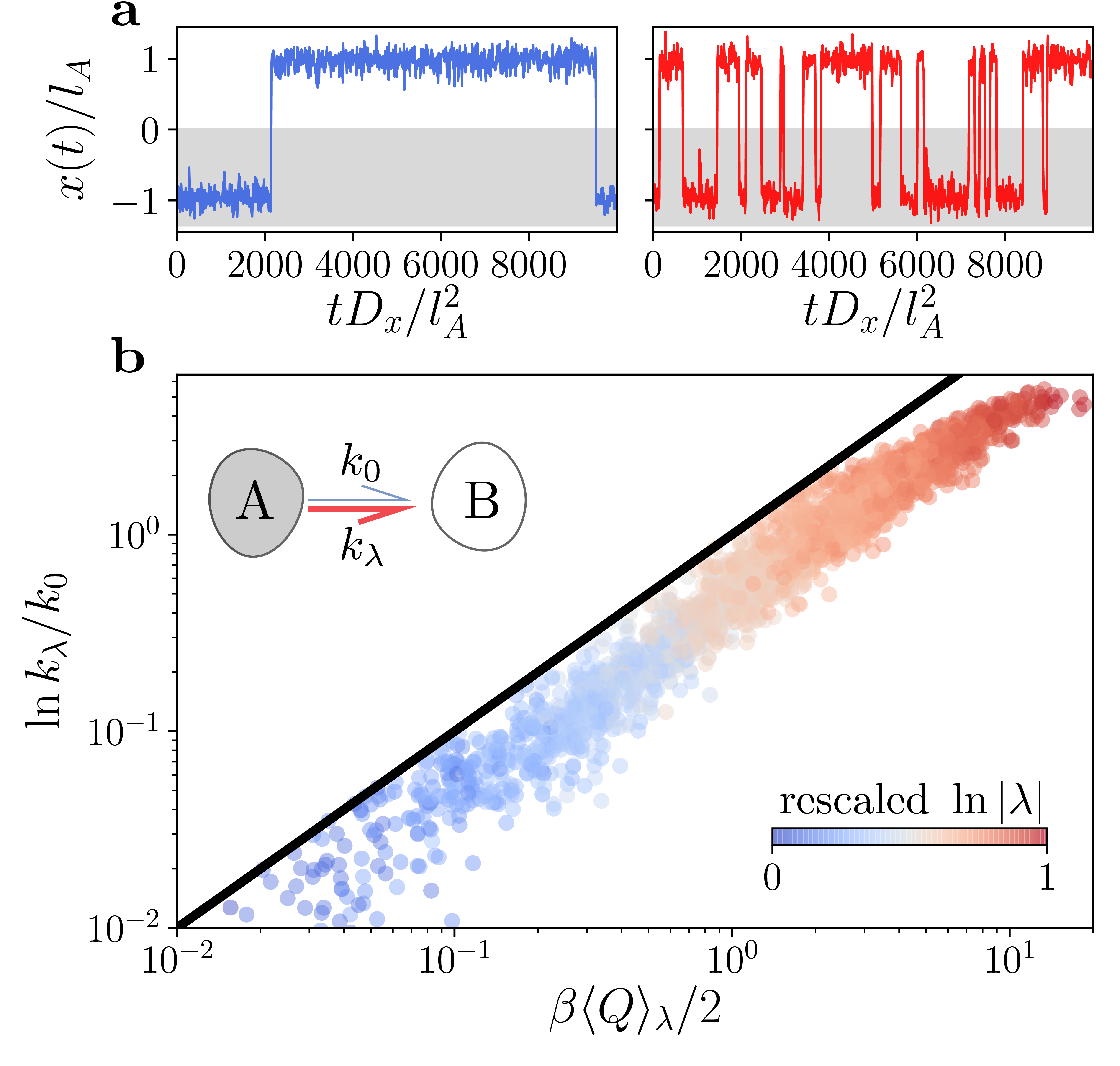
Figure 1: Nonequilibrium driving enhances transition rates. $\mathbf{a}$, Trajectories of a two-state system in equilibrium (left) and the same process driven away from equilibrium (right) by a time-dependent external force. $\mathbf{b}$, Rate enhancement for different asymmetric two-state systems as a function of dissipated heat, each driven by a randomly chosen combination of deterministic and stochastic external forces. The bound in Eq. 11 is shown as a black line and points are colored according to the magnitude of the force, low (blue) to high (red).

Autonomous and deterministic forcing

To illustrate the robustness of our dissipative bound, we first consider the overdamped dynamics of a particle in a one-dimensional asymmetric potential subject to both external time dependent and nonthermal forces. Specifically, the equation of motion for the position of the particle, $x$, is taken as $\gamma\dot{x}=-\partial_{x}V(x)+\lambda(t)+\sqrt{2k_{\mathrm{B}}T\gamma}\eta_{x}$ where $\gamma$ is the friction due to the surrounding medium, imposing a diffusion constant $D_{x}=k_{\mathrm{B}}T/\gamma$, and $\eta_{x}$ is a Gaussian random variable with $\langle\eta_{x}(t)\rangle=0$ and $\langle\eta_{x}(t)\eta_{x}(t^{\prime})\rangle=\delta(t-t^{\prime})$. The static external potential consists of two quartic states, $V(x)=V_{A}(x)\Theta(-x)+V_{B}(x)\Theta(x)$. Each basin $V_{i}(x)=(\Delta V_{i}x^{2}/(2l_{i}^{2}))(x^{2}/(2l_{i}^{2})-1)$, $i\in\{A,B\}$, is characterized by the distance of its minimum $(|x|,|y|)=(l_{i},\Delta V_{i})$ to the origin, where the states are joined by $\Theta(x)$, the Heaviside function. $V(x)$ supports two metastable states with a barrier between them if $\beta\Delta V_{i}>1$ for both $i=A$ and $B$. Figure. 1a), where $x(t)$ exhibits fluctuations concentrated around two regions of the potential, with few, fleeting transitions between them, manifests this metastability.

We drive the system out of equilibrium according to a time-dependent protocol $\lambda(t)=f[p\cos(\omega t)+(1-p)\cos(\theta(t))]$ with maximum amplitude $f$ partitioned, $p\in[0,1]$, into deterministic and autonomous components. The deterministic portion of the driving is periodic with frequency $\omega$, whereas the autonomous piece is determined by an additional nonthermal process, $\dot{\theta}(t)=\sqrt{2D_{\theta}}\eta_{\theta}$, with diffusion constant $D_{\theta}$, and delta-correlated white noise, $\langle\eta_{\theta}(t)\rangle=0$ and $\langle\eta_{\theta}(t)\eta_{\theta}(t^{\prime})\rangle=\delta(t-t^{\prime})$.

Considering transitions that take the particle from one side of the potential to the other, we define $h_{A}=\Theta(x+l_{A}/\sqrt{3})$ and $h_{B}=\Theta(x-l_{B}/\sqrt{3})$, which correspond to the locations of the maximum force opposing the transition in the absence of $\lambda(t)$. The dissipated excess heat can be computed from

$$Q(t)=\int^{t}_{0}dt^{\prime}\lambda(t)\dot{x}(t^{\prime}),$$ (12)

and its mean estimated within the nonequilibrium steady-state by integrating the dissipation rate over reactive trajectories of length $t$, given by the typical transition path time as discussed in Methods and Sec. S3. Given a suitable separation between inverse rate and relaxation time, $Q$ is often insensitive to the precise value of $t$. We reiterate that $Q$ differs from the total heat by the conservative boundary portion which appears in both the equilibrium and driven actions, and therefore does not play a role in the rate enchancement.

Figure 1b) shows the results of 3000 randomly constructed models, where $\Delta V_{i},l_{i}$, $p$, $f$, and $D_{\theta}$, were chosen uniformly over a wide range of parameters, as detailed in Methods. For each model, $k_{\lambda}$, $k_{0}$ and $\langle Q\rangle_{\lambda}$ have been independently evaluated, and Fig. 1b) demonstrates that the bound holds across the broad parameter-space. Points are colored blue to red in increasing magnitude of the driving force $f$, showing that the protocol most efficiently amplifies the equilibrium rate when $\beta\langle Q\rangle_{\lambda}<10$. Pushing past this regime, the bound becomes progressively weaker, as dissipation increases, but rate enhancement reaches a plateau. This corresponds to a limit where driving is large enough to degrade the assumption that basin $A$ is metastable.

In order to understand the physical processes that determine whether or not the bound is saturated, we focus on two cases of the model presented above. First, we set $p=0$, which corresponds to an active Brownian particle in an external potential. Active Brownian particles provide a canonical realization of how autonomous athermal noise can drive novel steady-states without simply imparting an effective temperature[16]. These self-propelled agents exhibit dynamical symmetry breaking and collective motion [17, 18], and previous studies have shown that the escape of active particles from a metastable potential exhibits interesting behavior arising from an interplay between the driving force, persistence time statistics, and the shape of the potential[19, 20]. For simplicity we take a symmetric potential, with $l_{A}=l_{B}=1$ and $\beta\Delta V_{A}=\beta\Delta V_{B}=10$, setting $\gamma=1$ and $k_{\mathrm{B}}T=1/2$.

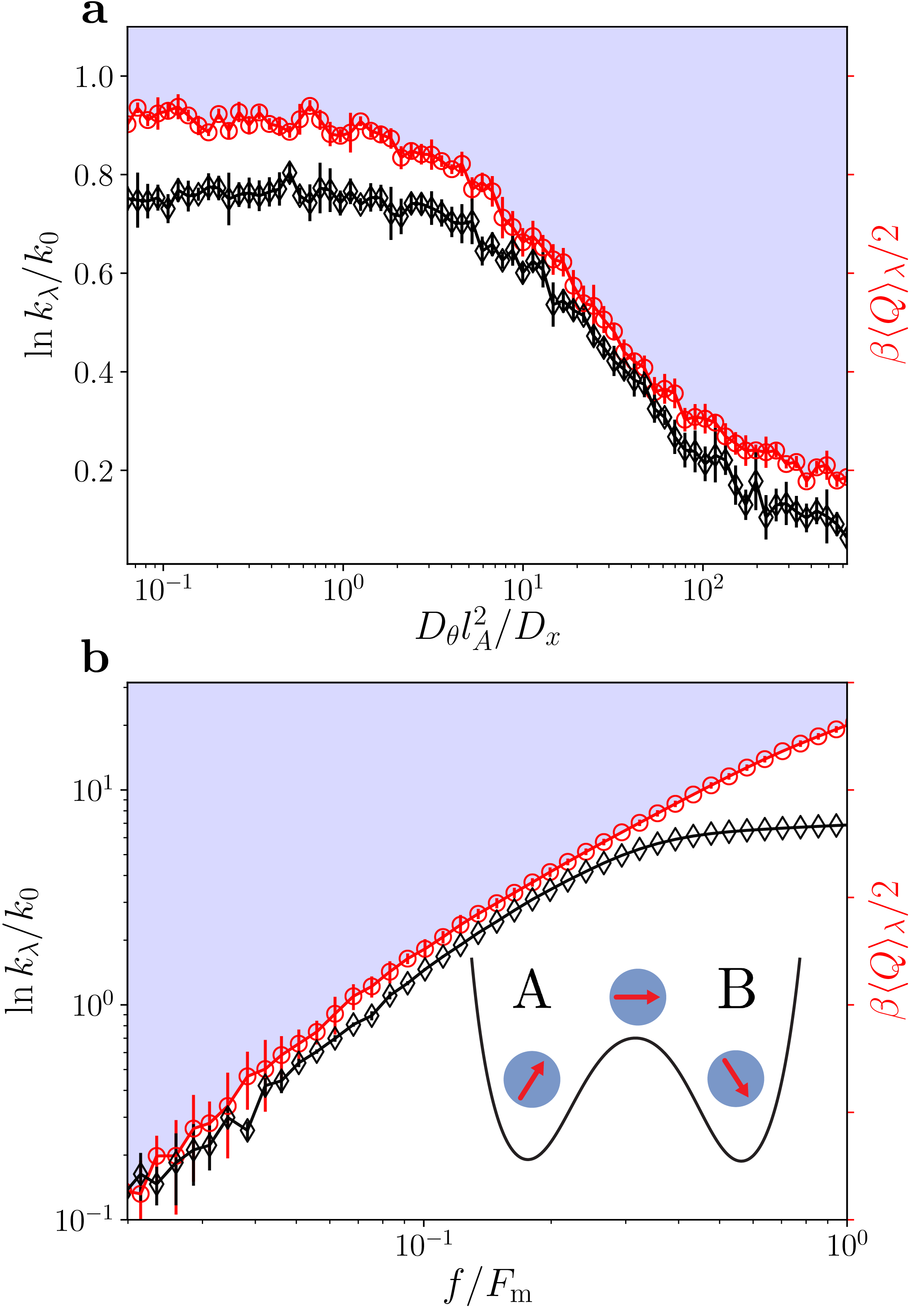
Figure 2: Rate enhancement for an active Brownian particle. a, Rate enhancement as a function of rotational diffusivity constant $D_{\theta}l_{A}^{2}/D_{x}$ for $f=1$. b, Rate enhancement as a function of the magnitude of active driving relative to the maximum force opposing the transition in equilibrium $f/F_{m}$ for $D_{\theta}=1/2$. In both, the rate enhancement (black diamonds) is bounded by the dissipated heat (red circles).

Figure 2a) shows the dependence of the rate enhancement on the rotational diffusivity, $D_{\theta}$ at fixed $f=1$. The small $D_{\theta}$ limit is a quasi-stationary regime corresponding to an equilibrium system with an additional linear force added to the potential. Increasing the rotational diffusivity decreases the persistence of the driving, and as a consequence $\langle Q\rangle_{\lambda}$ and $k_{\lambda}/k_{0}$ fall off in this limit. In the large $D_{\theta}$ limit, the system is effectively in equilibrium at an elevated temperature, as $\lambda$ averages to 0. Lower rate enhancement and little dissipation are observed across this range of $D_{\theta}$, and our bound is uniformly close. These results are consistent with a recent study in which an effective potential approach was used to derive $k_{\lambda}/k_{0}$ for an active Ornstein–Uhlenbeck process in a cubic well[21]. As shown in Fig. 2b), our bound is closest to the true rate enhancement when driving is small compared to the maximum force needed to surmount the barrier in equilibrium, $f<F_{\mathrm{m}}$ where $F_{m}=8\Delta V_{A}/3\sqrt{3l_{A}}$. In that regime, the heat and rate enhancement both scale with $f^{2}$, as predicted by linear response theory. When the protocol and gradient forces are comparable, the transition ceases being a rare event and further increasing $f$ has little effect on the rate, but increases the heat.

As a second test case, we consider underdamped dynamics with time-periodic driving, $p=1$. This model, known as the Duffing oscillator,[22] is the simplest model of a stochastic pump and one whose nonequilibrium behavior is marked by significant nonlinearity. As an underdamped process, its barrier crossing behavior is determined both by spatial as well as energy diffusion, in which both position and velocity correlations play a role. The equation of motion is given by $m\ddot{x}=-\gamma\dot{x}-\partial_{x}V(x)+\lambda(t)+\sqrt{2k_{\mathrm{B}}T}\eta_{x}$, where the mass $m$ reflects the change to underdamped dynamics. Again we take a symmetric potential, $l_{A}=l_{B}=1$, now with $\beta\Delta V_{A}=\beta\Delta V_{B}=14$ and $m=\beta=\gamma=D_{x}=1$.

Figure 3a) shows that for a moderate force, $f/F_{\mathrm{m}}\approx 0.13$, there is an optimal driving frequency, denoted here as $\omega^{*}$, which greatly enhances the transition rate. This phenomenon is known as stochastic resonance[22]. For slow driving, $\omega\ll\omega^{*}$, the particle typically makes a transition before the external force reaches its maximum. For $\omega\gg\omega^{*}$ driving is inefficient, and on average requires multiple forcing cycles before presenting a chance to cross the barrier with the help of a positive force within the time of a typical transition. The approximate shape of the rate enhancement profile is Lorentzian, a trait inherited from the absorption lineshape of an underdamped harmonic oscillator. In this case, the resonant frequency coincides with the curvature of the equilibrium double-well potential driven with a quasi-static force, $\omega^{*}\approx\sqrt{8(\Delta V-f)-\gamma^{2}/4}$[23]. We find near saturation of the bound throughout a wide range of frequencies and across even such nonlinear behavior as stochastic resonance. In Fig. 3b), we plot $k_{\mathrm{neq}}/k_{\mathrm{eq}}$ and $\beta\langle Q\rangle_{\lambda}/2$ against the driving amplitude relative to $F_{\mathrm{m}}$. As in the other examples, the bound on rate enhancement is tight so long as the metastability of state $A$ is preserved.

Thus far, we have characterized rates with transition paths, which lend themselves to a natural response theory for $\ln k_{\lambda}$, and therefore the ratio of rates. However, the survival probability $p_{\lambda}(t)=\exp(-k_{\lambda}t)=1-Z_{AB}(\lambda)/Z_{A}(\lambda)$ contains similar information in the case of two metastable states, when $h_{A}+h_{B}=1$. Falasco and Esposito recently[24] worked with this quantity to prove a speed limit on escape processes. Extending these results, we derive analogous bounds on absolute reaction rates (Sec. S4). Assuming rare rates, we bound the ratio of survival probabilities $p_{\lambda}(t)/p_{0}(t)$, and thus the difference of rates $k_{\mathrm{neq}}-k_{\mathrm{eq}}$, from above and below using the relative action and Jensen’s inequality. The final result reads

$$\beta\left\langle\Delta\dot{U}_{\lambda}\right\rangle_{\lambda}\leq k_{\lambda}-k_{0}\leq\beta\left\langle\Delta\dot{U}_{\lambda}\right\rangle_{0}$$ (13)

where the rate of change of the relative action forms an envelope around the change in the transition rate. If $k_{0}\ll k_{\lambda}$ then Eq. 13 acts as a speed limit on the forced process. On the other hand, if $k_{\lambda}\ll k_{0}$, Eq. 13 reports on the minimum dissipation required to slow down a fast equilibrium process. The envelope in Eq. 13 is similar to the bound derived by Falasco and Esposito in that it relates differences of rates to conditioned path ensemble averages. However, in Eq. 13, two forward rates under different dynamics are considered, while in Ref. [24] a forward rate is compared to its backward counterpart in the same ensemble. By considering a pair of rates explicitly related by time reversal symmetry, the result of Falasco and Esposito follows directly from the fluctuation theorem[11]. By contrast, the results presented in this work do not follow from the fluctuation theorem; rather, they are a result of trajectory ensemble reweighting.

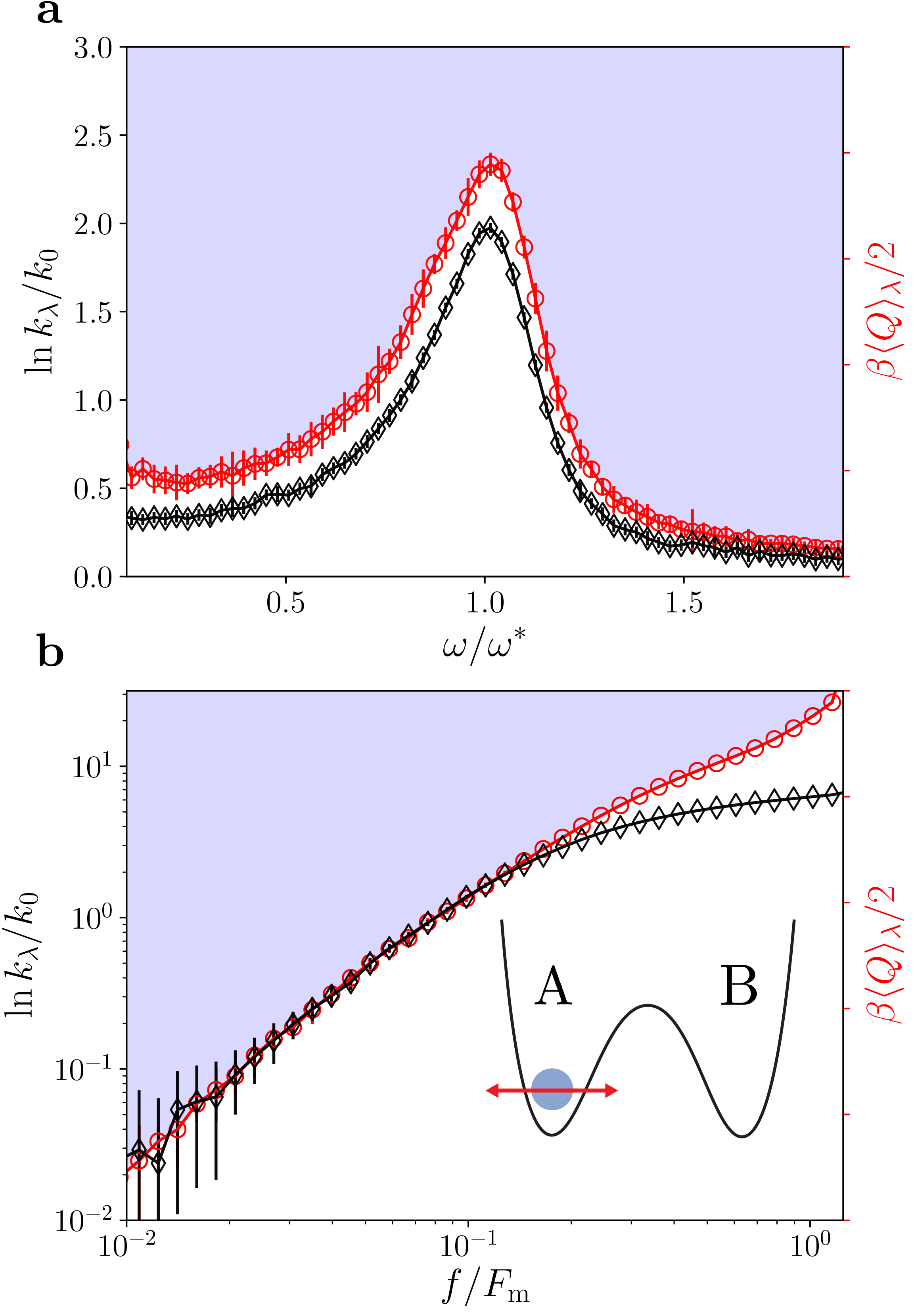
Figure 3: Rate enhancement in the Duffing oscillator. a, Rate enhancement as a function of the magnitude of driving frequency relative to the natural frequency of the equilibrium system, $\omega/\omega^{*}$, for $f=1.4$. b, Rate enhancement as a function of the magnitude of function of the periodic driving relative to the maximum force opposing the transition in equilibrium $f/F_{m}$ for $\omega/\omega^{*}=1$ at $f=1.4$. In both, the rate enhancement (black diamonds) is bounded by the dissipated heat (red circles).

The variational relationship in Eq. 11 between the transition rate and a thermodynamic quantity is reminiscent of equilibrium transition state theory, where the rate is bounded by the thermal flux times the probability that a thermal fluctuation brings the system from an initial reactant state to a rare transition state. From the Kawasaki distribution,[11] the nonequilibrium configurational distribution is related to the equilibrium one by a cumulant generating function of the excess dissipation conditioned on ending at a specific configuration. As explained in the Sec. S5, neglecting changes to the flux generated by coupling to a nonequilibrium process, the transition state theory estimate of the rate is bounded by the average heat conditioned on ending at the transition state. Eq.  11 thus has the interpretation of a nonequilibrium extension to standard transition state theory, and is expected to be a good approximation to the rate enhancement in cases where the system spends little time at the top of the barrier.

While our examples have focused on simple one dimensional models, our formalism is general and can be straightforwardly applied to many-body interacting systems. One immediate consequence of higher dimensionality is that unlike in the examples explored here, applied forces need not be aligned with the direction of the most likely transition path. In such cases, we expect the efficiency with which an arbitrarily applied force enhances the rate to be suppressed relative to the largely saturated bounds we have found here, as energy may be transduced into modes not correlated with overcoming the barrier. In light of our results, a natural optimal control problem arises in which nonequilibrium protocols can be constructed that minimize the dissipation for a given desired rate enhancement. Methods to perform such optimizations employing molecular simulation and importance sampling have been recently developed and show promise in complex systems [25, 26, 27]. Similarly, the protocols uncovered by such an optimization have the potential to lend mechanistic insight into reactions far from equilibrium, as basic concepts like free energy barriers and gradient flows cease being well defined. The effect of dissipation on rate enhancement under counter-diabatic [28] constraints, as well as in discrete-state networks and reaction-diffusion settings, remains to be seen.

Overall, our investigations build a general framework for the systematic and computationally efficient characterization of rate enhancement. Predicting how structure and external influence conspire to alter reaction rates far from equilibrium is of immediate importance in designing proteins, enzymes, small-molecule drugs, and the complex environments in which they operate. We foresee future studies in interacting colloidal and polymeric systems, both in shear and confining geometries that change dynamically in time [29]. Applications to heterogeneous growth, nucleation and jamming will also be interesting avenues to explore [30]. Time-dependent chemical potential gradients in gated release and receptor binding contexts, as well as designing interaction protocols [31] for quick and robust self-assembly [32] and pattern-formation [33] are another set of pressing examples to which our theory can apply. Local heating in ATP hydrolysis and facilitated diffusion on DNA[34], where electric fields play a pivotal role, are all more complex problems that may prove fruitful to study in this manner.

Methods

In our first main text example, we consider a double-well potential $V(x)$ pieced together continuously at $x=0$, and the parameters dictating its shape and the form of the driving are drawn uniformly. This is done $n$ times to create a parameter database (each entry labeled by integer $i$ from $0$ to $n-1$) before any simulations are run. Each point in Fig. 1, corresponds to a unique set of system parameters chosen as follows. Fixing $\beta=D_{x}=1$, we uniformly draw $\beta\Delta V_{A},\beta\Delta V_{\mathrm{B}}\in(3,7)$, $l^{2}_{\mathrm{i}}\in 8\Delta V_{\mathrm{i}}(\omega^{-2}_{\mathrm{max}},\omega^{-2}_{\mathrm{min}})$, $p\in[0,1]$, $\log f\in[-1,\log f_{\mathrm{max}}]$, and $D_{\theta}\in[0.1,10]$, where we constrain the natural frequencies of the wells to lie between $\omega_{\mathrm{min}}=3.5$ and $\omega_{\mathrm{min}}=7.5$.

Simulations for the overdamped systems studied, including the mixed driving system and the active barrier crossing, are propagated with a first order stochastic Euler integrator using a timestep of $\Delta t=10^{-2}$ in units of the $A$-state relaxation time $\tau_{A}=l_{A}/\sqrt{8\Delta V_{A}}$. For the underdamped Duffing oscillator calculations, we used a OVRVO[35] integrator, employing a symplectic 5-step Strang splitting of the time-evolution operator with the same time-step. Before turning $\lambda$ on at time zero, the dynamics are first evolved in equilibrium, $\lambda(t)=0$, for $t=1.5\times 10^{3}\Delta t$, to equilibrate. We calculate $k_{\lambda}$ and $k_{0}$ by counting the number of transitions from $A$ to $B$ and dividing by simulation time, $1.25-5\times 10^{7}\Delta t$. Transitions are counted when $x(t)$ passes from $A$ to $B$ and stays there at least order $2.75\Delta t$ steps without recrossing, which we find to yield consistent results with rates extracted from the side-side correlation function. We perform $24$ simulations, each of which yields a noisy estimate of the rate, and we record the mean and standard error bars.

We compute the time-dependent average $\left\langle Q\right\rangle_{\lambda}(t)$, independently of the rates, as follows. Using the same criteria for a transition as defined in the proceeding paragraph, we perform as many simulations as is needed to ensure sufficient statistics, which, depending on the specific system parameters, corresponds to $10^{3-4}$ transitions. At each point in time, we record the instantaneous rate of heat dissipation as well as an indicator function to coarse-grain $x(t)$ into either state $A$, state $B$, or the transition state, which in this example we define as $x\in A\cup B$, the intersection between states. Immediately after each simulation, we collect and save a list of times when transitions started, $t_{1}$, and ended, $t_{2}$. Once all simulations are complete, we histogram transition path times, $t_{2}-t_{1}$. We integrate over a discretized version of the heat flux in Eq. 12, $Q(t=n\Delta t)=\int_{0}^{t}dt^{\prime}\lambda(t^{\prime})\dot{x}(t^{\prime})\approx\sum^{n-1}_{i=0}\lambda_{i}(x_{i+1}-x_{i})$. In order to account for all transitions, we choose an initial observation time $t$ equal to that required for $99\%$ of transition paths to proceed start to finish. For each transition, we position a window of length $t$ so that it ends immediately after $t_{2}$, and integrate over it. We slide this window to the right by $O(10\Delta t)$ steps and integrate again, repeating until the endpoints of the window . The coarse-grained time $\approx\Delta t$ controls how highly correlated reactive trajectories are. Choosing it is thus some what of an art in the sense that when very small, one must integrate over many more paths, but if it is too large, $\left\langle Q\right\rangle_{\lambda}$ will have greater statistical error. If, at any point, a window passes through a transition region without seeing a transition, due to coarse-graining, the observation time is increased by a small factor of $t\mapsto t(1+1/4)$ and the integration is restarted from the beginning.

The rates are small quantities, prone to high statistical uncertainty which is amplified when the log of their ratio is taken. Because of this, we rerun all points that have greater standard error, in either enhancement or dissipation, than the mean. The majority or these points correspond to lightly forced systems where the maximum protocol amplitude is usually much smaller than the thermal energy scale, $\beta|\lambda|\sim 10^{-1}$. In this regime, $\ln k_{\lambda}/k_{0}\ll 1$, is well within linear response. Since we are focused on the case where the equilibrium rate changes appreciably, and know that by time-reversal symmetry arguments, the only contribution in this near-equilibrium case comes from dissipation, throughout the main text we only show points with $\ln k_{\lambda}/k_{0}$ larger than a small number, which we choose to be $10^{-2}$.

Acknowledgments: This material is based upon work supported by the National Science Foundation under grant no. CHE-1954580 and by a Scialog Program sponsored jointly by Research Corporation for Science Advancement and the Gordon and Betty Moore Foundation.

References

References

- Bustamante et al. [2004] C. Bustamante, Y. R. Chemla, N. R. Forde, and D. Izhaky, “Mechanical processes in biochemistry,” Annu. Rev. Biochem. 73, 705 (2004).
- Mugnai et al. [2020] M. L. Mugnai, C. Hyeon, M. Hinczewski, and D. Thirumalai, “Theoretical perspectives on biological machines,” Rev. Mod. Phys. 92, 025001 (2020).
- Mashaghi et al. [2014] A. Mashaghi, G. Kramer, D. C. Lamb, M. P. Mayer, and S. J. Tans, “Chaperone action at the single-molecule level.” Chem. Rev. 114, 660 (2014).
- Wu et al. [2009] Y. L. Wu, D. Derks, V. van Blaaderen, and A. Imhof, “Melting and crystallization of colloidal hard-sphere suspensions under shear,” Proc. Natl. Acad. Sci. 106, 10564 (2009).
- Chandler [1978] D. Chandler, “Statistical mechanics of isomerization dynamics in liquids and the transition state approximation,” J. Chem. Phys. 68, 2959 (1978).
- Kramers [1940] H. Kramers, “Brownian motion in a field of force and the diffusion model of chemical reactions,” Physica 7, 284 (1940).
- Bouchet and Reygner [2016] F. Bouchet and J. Reygner, “Generalisation of the eyring–kramers transition rate formula to irreversible diffusion processes.” Ann. Inst. Henri Poincaré 17, 3499 (2016).
- Bolhuis et al. [2002] P. G. Bolhuis, D. Chandler, C. Dellago, and P. L. Geissler, “Transition path sampling: Throwing ropes over rough mountain passes, in the dark.” Annu. Rev. Phys. Chem. 53, 291 (2002).
- Seifert [2012] U. Seifert, “Stochastic thermodynamics, fluctuation theorems and molecular machines,” Rep. Prog. Phys. 75, 126001 (2012).
- Jarzynski [1997] C. Jarzynski, “Nonequilibrium equality for free energy differences,” Phys. Rev. Lett. 78, 2690 (1997).
- Crooks [2000] G. Crooks, “Path ensembles averages in systems driven far-from-equilibrium.” Phys. Rev. E. 61, 2361 (2000).
- Horowitz and Gingrich [2020] J. M. Horowitz and T. R. Gingrich, “Thermodynamic uncertainty relations constrain non-equilibrium fluctuations,” Nat. Phys. 16, 15 (2020).
- Onsager and Machlup [1953] L. Onsager and S. Machlup, “Fluctuations and irreversible processes.” Phys. Rev. 91, 1505 (1953).
- Maes [2020] C. Maes, “Frenesy: time-symmetric dynamical activity in nonequilibria.” Phys. Rep. 850, 1 (2020).
- Gao and Limmer [2019] C. Y. Gao and D. T. Limmer, “Nonlinear transport coefficients from large deviation functions.” J. Chem. Phys. 151, 014101 (2019).
- Cates and Tailleur [2013] M. E. Cates and J. Tailleur, “When are active brownian particles and run-andtumble particles equivalent? consequences for motility-induced phase separation,” EPL 101, 20010 (2013).
- Nemoto et al. [2019] T. Nemoto, E. Fodor, M. E. Cates, R. L. Jack, and J. Tailleur, “Optimizing active work: Dynamical phase transitions, collective motion, and jamming.” Phys. Rev. E. 99, 022605 (2019).
- GrandPre and Limmer [2018] T. GrandPre and D. T. Limmer, “Current fluctuations of interacting active brownian particles.” Phys. Rev. E. 98, 060601 (2018).
- Woillez et al. [2019] E. Woillez, Y. Zhao, Y. Kafri, V. Lecomte, and J. Tailleur, “Activated escape of a self-propelled particle from a metastable state.” Phys. Rev. Lett. 122, 258001 (2019).
- Woillez et al. [2019] E. Woillez,Y. Kafri, and V. Lecomte, “Nonlocal stationary probability distributions and escape rates for an active Ornstein–Uhlenbeck particle.” J. Stat. Mech. 2020, 063204 (2020).
- Sharma, Wittmann, and Brader [2019] A. Sharma, R. Wittmann, and J. M. Brader, “Escape rate of active particles in the effective equilibrium approach.” Phys. Rev. E. 122, 258001 (2019).
- Gammaitoni et al. [1998] L. Gammaitoni, P. Hanggi, P. Jung, and F. Marchesoni, “Stochastic resonance,” Rev. Mod. Phys. 70, 223 (1998).
- Jung [1993] P. Jung, “Periodically driven stochastic systems,” Phys. Rep. 234, 175 (1993).
- [24] G. Falasco and M. Esposito, “Dissipation-time uncertainty relation.” Phys. Rev. Lett. 125, 120604 (2020).
- Chetrite and Touchette [2015] R. Chetrite and H. Touchette, “Nonequilibrium markov processes conditioned on large deviations.” Ann. Inst. Henri Poincaré 16, 2005 (2015).
- Das and Limmer [2019] A. Das and D. T. Limmer, “Variational control forces for enhanced sampling of nonequilibrium molecular dynamics simulations.” J. Chem. Phys. 151, 244123 (2019).
- Gringrich et al. [2016] T. R. Gringrich, G. M. Rotskoff, G. E. Crooks, and P. L. Geissler, “Near-optimal protocols in complex nonequilibrium transformations,” Proc. Natl. Acad. Sci. 113, 10263 (2016).
- [28] S. Iram, E. Dolson, J. Chiel, J. Pelesko, N. Krishnan, O. Güngör, B. Kuznets-Speck, S. Deffner, E. Ilker, J. G. Scott, and M. Hinczewski, “Controlling the speed and trajectory of evolution with counterdiabatic driving.” Nat. Phys. (2020) .
- Schneider et al. [2007] S. W. Schneider, S. Nuschele, A. Wixforth, C. Gorzelanny, A. Alexander-Katz, R. R. Netz, and M. F. Schneider, “Shear-induced unfolding triggers adhesion of von willebrand factor fibers,” Proc. Natl. Acad. Sci. 104, 7899 (2007).
- Delarue et al. [2016] M. Delarue, J. Hartung, C. Schreck, P. Gniewek, L. Hu, S. Herminghaus, and O. Hallatschek, “Self-driven jamming in growing microbial populations,” Nat. Phys. 12, 762 (2016).
- Rogers, Shih, and Manoharan [2016] W. B. Rogers, W. M. Shih, and V. N. Manoharan, “Using DNA to program the self-assembly of colloidal nanoparticles and microparticles,” Nat. Rev. Mater. 1, 16008 (2016).
- Aubret et al. [2018] A. Aubret, M. Youssef, S. Sacanna, and J. Palacci, “Targeted assembly and synchronization of self-spinning microgears,” Nat. Phys. 14, 1114 (2018).
- Denk et al. [2018] J. Denk, S. Kretschmer, J. Halatek, C. Hartl, P. Schwille, and E. Frey, “MinE conformational switching confers robustness on self-organized min protein patterns,” Proc. Natl. Acad. Sci. 115, 4553 (2018).
- Liu et al. [2016] J. Liu, J. Hanne, B. M. Britton, J. Bennett, D. Kim, J. B. Lee, and R. Fishel, “Cascading MutS and MutL sliding clamps control dna diffusion to activate mismatch repair,” Nature 539, 583 (2016).
- Sivak, Chodera, and Crooks [2014] D. A. Sivak, J. D. Chodera, and G. E. Crooks, “Time step rescaling recovers continuous-time dynamical properties for discrete-time langevin integration of nonequilibrium systems,” J. Phys. Chem. B 118, 6466 (2014).