On the Environments of Giant Radio Galaxies

Abstract

We test the hypothesis that environments play a key role in enabling the growth of enormous radio structures spanning more than 700 kpc, an extreme population of radio galaxies called giant radio galaxies (GRGs). To achieve this, we explore (1) the relationships between the occurrence of GRGs and the surface number density of surrounding galaxies, including satellite galaxies and galaxies from neighboring halos, as well as (2) the GRG locations towards large-scale structures. The analysis is done by making use of a homogeneous sample of 110 GRGs detected from the LOFAR Two-metre Sky Survey in combination with photometric galaxies from the DESI Legacy Imaging Surveys and a large-scale filament catalog from the Sloan Digital Sky Survey. Our results show that the properties of galaxies around GRGs are similar with that around the two control samples, consisting of galaxies with optical colors and luminosity matched to the properties of the GRG host galaxies. Additionally, the properties of surrounding galaxies depend on neither their relative positions to the radio jet/lobe structures nor the sizes of GRGs. We also find that the locations of GRGs and the control samples with respect to the nearby large-scale structures are consistent with each other. These results demonstrate that there is no correlation between the GRG properties and their environments traced by stars, indicating that external galaxy environments are not the primary cause of the large sizes of the radio structures. Finally, regarding radio feedback, we show that the fraction of blue satellites does not correlate with the GRG properties, suggesting that the current epoch of radio jets have minimal influence on the nature of their surrounding galaxies.

1 Introduction

Over the past two decades, feedback from supermassive black holes has been considered as a fundamental mechanism in galaxy formation theory in order to reproduce the observed properties of galaxies (e.g., Benson et al., 2003; Schaye et al., 2015; Davé et al., 2019; Nelson et al., 2019). Supermassive black holes are expected to remove a substantial mass of gas from galaxies and thereby quench star formation. In addition, supermassive black holes are expected to maintain the heat content of gas around quenched galaxies to prevent gas cooling for further star-formation activity (e.g., Silk & Rees, 1998; Bower et al., 2008; Alexander & Hickox, 2012; McNamara & Nulsen, 2012; Chen et al., 2019; Hardcastle et al., 2019).

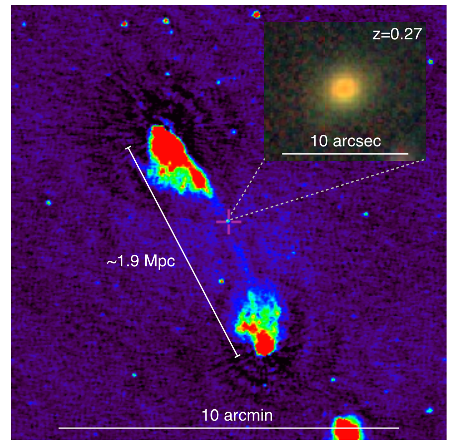
One of the observed form of black hole feedback is extended radio jets and lobes emerging from the centers of galaxies (e.g., Worrall, 2009; Best & Heckman, 2012; Fabian, 2012; McNamara & Nulsen, 2012). Since their discovery, radio galaxies have been classified into different types according to their morphological structure of radio emission (e.g., Fanaroff & Riley, 1974; Hardcastle & Croston, 2020). A small fraction of radio galaxies ($\sim 5\%$) possess extremely extended radio-emission extending far beyond the size of dark matter halos and are referred to as giant radio galaxies (GRGs), (e.g., Willis et al., 1974; Saripalli et al., 1986; Mack et al., 1998; Ishwara-Chandra & Saikia, 1999). These GRGs are roughly defined as radio galaxies with linear projected distances between two radio lobes of greater than 700 kpc (See Figure 1 as an example). Given the extreme properties of GRGs, it is surmised that understanding the nature and origin of GRGs will illuminate the physical mechanisms of black hole feedback on galaxy formation.

Previous studies have suggested two main scenarios that allow radio galaxies to grow to such large scales: (1) They can be produced by either powerful engines within normal timescales ($\sim 10-100$ Myr) (e.g., Gopal-Krishna et al., 1989) or modest energy with prolonged timescales or multiple phases of activity (e.g., Subrahmanyan et al., 1996; Hardcastle et al., 2019; Bruni et al., 2020); (2) They tend to live in relatively low density environments which allows the radio lobes to grow to very large scales (e.g., Mack et al., 1998; Malarecki et al., 2015). While previous studies have explored both these scenarios, the origin(s) of GRGs are still not well understood. This is primarily due to their rare and difficult detection lending to small sample sizes. Therefore, previous results are based on the properties of only a handful of GRGs.

In the past few years, large radio surveys have increased the sample size of GRGs. For example, Kuźmicz et al. (2018) compile a sample of $\sim 300$ GRGs from all the previous observations and Dabhade et al. (2017) and Dabhade et al. (2020a) detect $\sim 200$ new GRGs from the NVSS dataset (Condon et al., 1998). Additionally, based on the DR1 data of the LOFAR Two-metre Sky Survey (LoTSS, Shimwell et al., 2019), Dabhade et al. (2020b) compile a sample of $\sim 200$ GRGs covering a wide range of redshift. These new GRG samples offer the opportunity to better characterize the properties of GRGs and their surrounding environments.

In this work, we will test the hypothesis that GRGs tend to live in low density environments by measuring the environments of GRGs as a function of redshift. To this end, we will make use of a GRG catalog compiled from the LoTSS and data from large optical surveys, including the imaging Surveys for the Dark Energy Spectroscopic Instrument (DESI) (Dey et al., 2019) and the Sloan Digital Sky Survey (York et al., 2000). The results will provide strict constraints on this hypothesis and thereby shed new light on the driving factors for the enormous sizes of GRGs. The structure of the paper is as follows. Our data analysis is described in Section 2. We show our results and discuss their implications in Section 3 and Section 4. We summarize in Section 5. Throughout the paper we adopt a flat $\Lambda$CDM cosmology with $h=0.7$ and $\Omega_{\rm M}=0.3$. When referring to distances, we use physical distances.

Figure 1: Radio image of a giant radio galaxy at $z\sim 0.27$ from the LOFAR Two-metre Sky Survey. The projected linear distance between the two radio lobes is approximately 1.9 Mpc. The optical image of the host galaxy (drawn from the DESI Legacy Imaging Surveys) is shown on the upper right corner.

Figure 2: Magnitude, stellar mass, and redshift distributions of the GRG host galaxies (blue) and the radio (green) and optical (red) control samples.

2 Data Analysis

To investigate the local and large-scale environments of GRGs, we apply statistical cross-correlation analyses to a large GRG catalog, a photometric galaxy catalog and a large-scale filament catalog. By doing so, we are able to quantify the local and large-scale environments of GRGs and compare the measurements with that of the control samples. Our approach, therefore, is to isolate whether the presence of bright and highly extended radio emission is correlated with the underlying galactic environment. In what follows, we describe the data sets and methods we use.

2.1 Datasets

• Giant radio galaxy catalog: We make use of a large, homogeneous giant radio galaxy catalog compiled by Dabhade et al. (2020b). This sample is obtained from the 1st data release of the LOFAR Two-metre Sky Survey (LoTSS, Shimwell et al., 2019; Williams et al., 2019), consisting of 239 GRGs from $z\sim 0$ up to $z\sim 1$. These GRGs are identified from the LoTSS pipeline assisted by visual inspections.

  To construct control samples as described in Section 2.2, we select GRGs that have (1) spectroscopic redshifts of their host galaxies identified in the 14th data release of the Sloan Digital Sky Survey (SDSS, York et al., 2000; Abolfathi et al., 2018) and (2) imaging observations covered by the DESI Legacy Imaging Surveys (Dey et al., 2019). We exclude 40 SDSS sources identified as quasars. This yields a sample of 110 GRGs for our analysis. As an example, Figure 1 shows the LOFAR radio image of a GRG and the corresponding optical image (g, r, and z bands) of the host galaxy.

• Photometric galaxy catalog: To investigate the local galaxy environments of GRGs, we use the DR8 photometric galaxy catalog of the DESI Legacy Imaging Surveys (the DESI Legacy Surveys, Dey et al., 2019). The catalog contains $\sim 10^{9}$ galaxies over $\sim 14,000\,\rm deg^{2}$ of the sky with photometric properties of $g$, $r$, $z$ and WISE channel 1, 2, 3, 4 bands (Wright et al., 2010) characterized by the Tractor algorithm (Lang et al., 2016). The limiting magnitudes of the DESI Legacy Surveys are about $24$, $23.4$ and $22.5$ for $g$, $r$, and $z$ bands respectively. These depths are sufficient for our purposes of detecting $L^{*}$ galaxies up to $z\sim 1$.

• Large-scale filament catalog: For exploring the locations of GRGs with respect to the large-scale structure, we use a filament catalog from Chen et al. (2016). The filamentary structures are identified based on a statistical algorithm for detecting density ridges (Chen et al., 2015) applied to the SDSS spectroscopic galaxy sample. The filament catalog includes random points sampled from the filaments as a function of redshift up to redshift 0.7 with 0.05 redshift intervals.

2.2 Properties of the GRG host galaxies

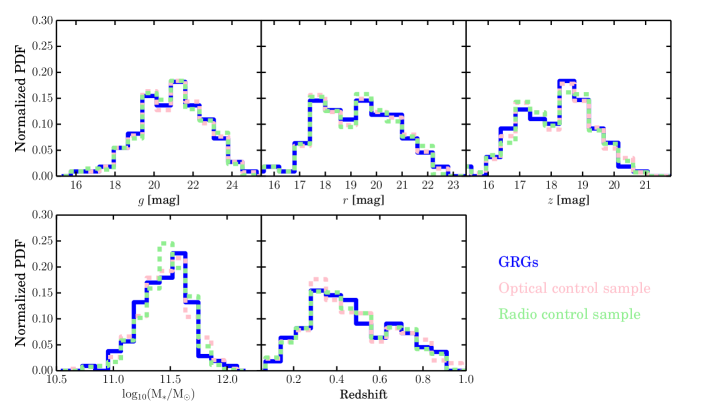
We summarize the properties of the GRG host galaxies in Figure 2, which shows the magnitude, stellar mass, and redshift distributions of the host galaxies. The stellar masses of the GRG host galaxies are obtained via spectral energy distribution (SED) fittings with the CIGALE package (Boquien et al., 2019). We adopt the simple stellar population from Bruzual & Charlot (2003) with Chabrier initial mass function (Chabrier, 2003) and delayed-exponential star-formation history. The best-fit stellar mass is constrained by the observed flux in $g$, $r$, $z$, WISE 1 and WISE 2 bands.

Similar to the host galaxies of typical radio-AGN galaxies (e.g., Best et al., 2005; Lin et al., 2010), the GRG host galaxies are massive red galaxies with $M_{*}>10^{11}\,M_{\odot}$. The corresponding typical dark matter halo mass is therefore a few times of $10^{13}\,M_{\odot}$ and the virial radius is approximately 500-600 kpc (e.g., Tinker et al., 2017). About 10% of GRGs are located in dark matter halos with even higher masses ($>10^{14}\,M_{\odot}$), i.e.  galaxy cluster environments (e.g., Dabhade et al., 2020b).

Figure 3: Top: Average number of galaxies around GRGs (blue) and around random positions (grey) within 600 kpc as a function of $z$-band magnitude and redshift. The difference between the two shows the contribution from satellite galaxies associated with GRGs as shown by blue data points in the bottom panel. Bottom: Magnitude distribution of satellite galaxies around GRGs. The red and green shaded regions show the same measurements around the optical and radio control samples respectively. The magnitude distributions of satellite galaxies around GRGs are consistent with the distributions around the two control samples.

2.3 Control samples

To evaluate whether or not GRGs tend to live in special environments, we construct two control samples that have similar optical photometric properties and redshifts as the GRG host galaxies. One sample is selected to have radio-emission detected in LoTSS with integrated flux greater than 0.2 mJy and the other is primarily selected to have no LOFAR detection. When combined, we can examine whether the presence of any radio emission is correlated to galaxy environments. In the following, we describe the two control samples in detail:

1. Radio control sample: To construct the radio control sample, we first cross-match SDSS DR14 spectroscopic galaxies with radio sources detected in LoTSS (Williams et al., 2019; Duncan et al., 2019), excluding the GRGs in the sample. This radio-optical sample consists of approximately 30,000 objects. For each GRG, we then select five galaxies from this radio-detected SDSS galaxy sample as the corresponding radio control galaxies. These control galaxies are selected with redshifts, $g$, $r$, $z$ band magnitudes, and morphology type matched to that of the host galaxy of the GRG. Specifically, these lie within 0.025 difference in redshift and 0.05 magnitude difference in each band. If fewer than 5 galaxies satisfied this selection criteria, we increase the redshift range by $20\%$ and magnitude difference by 0.05 iteratively.

2. Optical control sample: To construct the optical control sample, we make use of SDSS DR14 spectroscopic galaxies located between $\rm 162<RA<235$ deg and $\rm 46<DEC<56.5$ deg, approximately the sky region covered by the LoTSS DR1. We then exclude all of the SDSS galaxies detected in the DR1 LoTSS catalog. This process reduces the sample size by $\sim 10\%$. This optical sample consists of about 240,000 objects. For each GRG, we select five galaxies from this optical SDSS galaxy sample that satisfy the same criteria listed above for the radio control sample. We note that about $10\%$ of the optical selected region is not covered by the DR1 LoTSS. Therefore, $10\%$ of galaxies in the optical control sample are selected without radio information. Nevertheless, with the LoTSS radio detection rate of SDSS sources $(\sim 10\%)$, the contamination rate of radio emission in this optical control sample is expected to be nearly negligible (i.e. $\sim 1\%$).

By performing the same analysis to the GRG sample and the two control samples, we will compare the galaxy environment properties as a function of the extension of radio emission with fixed optical properties of host galaxies. Figure 2 shows the magnitude, stellar mass, and redshift distributions of the GRG host galaxies, the optical control sample and the radio control sample in blue, red, and green respectively. The stellar masses of galaxies in the control samples are obtained via SED fittings as described in Section 2.2.

2.4 Methods

We focus on two statistical measurements to characterize the environments of GRGs. The first one is the surface number density of surrounding galaxies associated with GRGs obtained by statistically subtracting the number density of coincident background and foreground galaxies. We perform the measurements from 20 kpc to 2 Mpc in projected distances, which include satellite galaxies bounded within the host halos of GRGs (the so-called “1-halo term”) and galaxies from neighboring halos (2-halo term). Given that the properties of satellites are the primary concern of the analysis, we will refer to these measurements as the distributions of satellites for simplicity.

The second measurement is the distances between GRGs and the nearest filamentary structures, which are identified from the SDSS spectroscopic galaxies. The typical scale involved is $\sim 10$ Mpc, several times larger than the satellite measurements. We use this GRG-filament distance measurement to infer the location of GRGs in the context of large-scale structure. In the following, we will describe the methods we apply for these two measurements respectively.

2.4.1 Cross-correlation method for estimating the number of satellite galaxies

To obtain the number density of satellite galaxies, we cross-correlate the GRG sample with the photometric galaxies detected from the DESI Legacy Surveys. For each GRG, we search and count the number of the surrounding photometric galaxies within a given (physical) impact parameter. The impact parameters are estimated by assuming that all the surrounding galaxies are at the same redshift of the GRG. The number of photometric galaxies around a given GRG, $\rm N_{gal}^{GRG}$, consists of two components: (1) satellite galaxies truly (physically) associated with the GRG, $\rm N_{sat}^{GRG}$, and (2) coincident background and foreground galaxies located at different redshifts, $\rm N_{coincident}$,

$$\rm N_{gal}^{GRG}=N_{sat}^{GRG}+N_{coincident}.$$ (1)

For each GRG, we estimate the average number of coincident background and foreground galaxies, $\rm\langle N_{coincident}\rangle$, based on the number of galaxies around 10 random positions in the sky footprint between $\rm 162<RA<228$ deg and $\rm 46<DEC<56.5$ deg. By subtracting $\rm\langle N_{coincident}\rangle$ from $\rm N_{gal}^{GRG}$, we can obtain the number of satellite galaxies associated with the GRG, $\rm N_{sat}^{GRG}$, without any spectroscopic redshift information of the photometric galaxies (e.g., Lan et al., 2016). Finally, we calculate the average number of satellite galaxies associated with the full set of GRGs to reduce Poisson uncertainty which dominates the number counts of individual sightlines,

$$\rm\langle N_{sat}^{GRG}\rangle=\frac{\sum\limits_{i=1}^{N_{GRG}}N_{sat}^{GRG,i}}{N_{GRG}},$$ (2)

where $\rm N_{GRG}$ is the number of GRGs used in the analysis.

Figure 4: Radial distributions of satellite galaxies around GRGs (blue), the optical control sample (red), and the radio control sample (green) as a function of redshift and stellar mass. The y-axis shows the surface number density of galaxies and the x-axis the impact parameters. The redshifts of the host galaxies increase from the left to the right panels. The upper and lower panels show the distribution for satellites with $M_{*}>10^{10.3}\,M_{\odot}$ and $10^{9.8}<M_{*}<10^{10.3}\,M_{\odot}$ respectively. The satellite radial distributions around GRGs and the two control samples are consistent with each other, indicating that GRGs do not preferentially live in lower density environments.

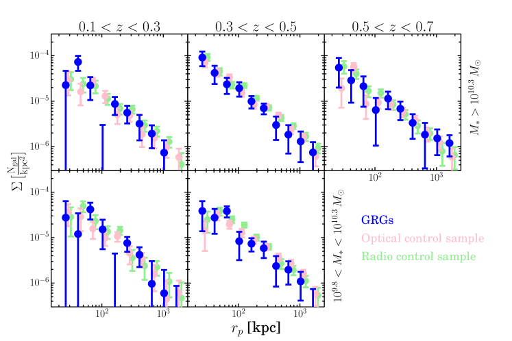
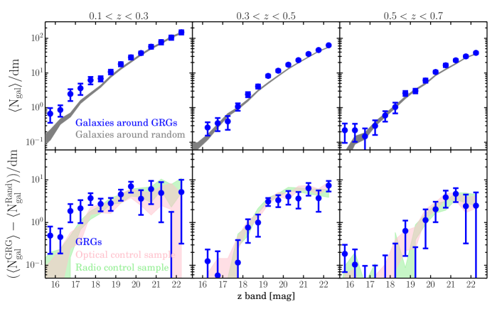
Figure 3 illustrates the method. In the upper panel, we show the average number of galaxies around GRGs (blue) and random positions (grey) within 600 kpc as a function of $z$-band magnitude and redshift. The lower panel shows the differences between the number counts around GRGs and around random positions. As can be seen, there are more galaxies around GRGs than around random positions. The difference results from the presence of satellite galaxies around GRGs. Additionally, the $z$-band magnitude distribution of these satellite galaxies becomes fainter towards higher redshifts. This trend confirms that the signal is only from satellite galaxies associated with GRGs. We find the number of satellites around GRGs within 600 kpc is similar to the number of satellites in dark matter halos with $\sim 10^{13.5}-10^{13.9}M_{\odot}$ as shown in Lan et al. (2016), similar to the halo masses inferred from the stellar mass of the host galaxies. We note that this method has been applied to many other research areas, such as measuring the conditional luminosity functions of groups and clusters (e.g., Lin et al., 2004; Lan et al., 2016; Tinker et al., 2019), detecting the splash-back radius of dark matter halos (e.g., More et al., 2016), and probing galaxies associated with absorption line systems (e.g., Lan et al., 2014; Lan, 2020).

Figure 5: Radial distributions of satellite galaxies with $M_{*}>10^{10.3}\,M_{\odot}$ around GRGs (blue) and the optical (red) and radio (green) control samples at redshift $0.1<z<0.7$. The inset shows the best-fit surface number density at 100 kpc for the three samples. The best-fit value for GRGs is consistent with the optical and radio control samples, indicating that the local galaxy environments of GRGs is mostly driven by the optical properties of the host galaxies.

In the lower panel of Figure 3, we also show the magnitude distributions of satellite galaxies around the optical and radio control samples with the shaded red regions and green regions respectively. As can be seen, the satellite magnitude distributions of the two control samples are consistent with that of the GRG sample. We will make quantitative comparisons in Section 3. We note that we estimate the uncertainty by bootstrapping the sample 500 times.

This method can be applied to explore any properties of galaxies associated with GRGs. Instead of the observed brightness of galaxies, we will explore the properties of satellite galaxies as a function of stellar mass. This will enable an examination of the full sample across redshift. To obtain the stellar mass of each galaxy, we use the CIGALE package (Boquien et al., 2019) assuming that each photometric galaxy is at the same redshift of the corresponding GRG. We adopt the same approach as described in Section 2.2, with the best-fit stellar masses constrained by the observed fluxes in the $g$, $r$, $z$, WISE 1 and WISE 2 bands. Note that in our analysis, we focus on the stellar mass of galaxies in a relative sense. Therefore, the absolute systematic uncertainty of stellar mass introduced by the adopted assumptions of stellar population modeling do not affect our results.

2.4.2 Distances between GRGs and the nearest filaments

To better understand the large-scale structure environments in which GRGs reside, we measure the distance between each GRG and the nearest filament structure from the filament catalog. The filaments are identified based on SDSS spectroscopic galaxies within the same redshift bin with a 0.05 redshift interval. Therefore, for each GRG, we extract filaments with the corresponding redshift bin and calculate the projected distance between the GRG and the nearest filament structure. We perform the same calculation for the control samples and compare the results between the three samples. The results will be described in Section 3.

3 Results

In this section, we will first present the distribution of satellite galaxies around GRGs and their control samples. We will also show the number of satellite galaxies around GRGs as a function of the properties of GRGs. Finally, we will present the environments in which GRGs reside in the context of large-scale structure.

3.1 Radial distributions of satellite galaxies around GRGs and around the control samples

Figure 4 shows the surface number density of satellite galaxies $\Sigma(r_{p})=\rm\langle N_{sat}^{GRG}\rangle/area$, around GRGs and the control samples as a function of impact parameter $(r_{p})$, redshift and stellar mass. Here we probe the impact parameters from $20$ kpc to $2$ Mpc, which includes satellite galaxies within the virial radius ($\sim 600$ kpc) of the GRG halos and galaxies in neighboring halos (the two-halo term). As can be seen, the radial distributions of satellite galaxies around GRGs and the control samples are consistent with each other across redshift and stellar mass. For the rest of the paper, we focus on the distribution of satellites with $M_{*}>10^{10.3}\,M_{\odot}$, a stellar mass range that is complete to redshift 0.7 and is an order of magnitude less than the stellar mass of the GRG host galaxies (Figure 2).

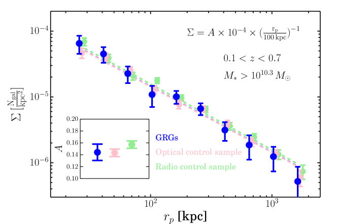
In Figure 5, we show the radial distributions of satellites with $M_{*}>10^{10.3}\,M_{\odot}$ around GRGs and the two control samples with $0.1<z<0.7$. We fit the satellite distributions with

$$\Sigma(r_{p})=A\times 10^{-4}\bigg{(}\frac{r_{p}}{100\,\rm kpc}\bigg{)}^{-1},$$ (3)

where $A$ is the surface number density of satellite galaxies at 100 kpc. We fix the power index as -1 given that the best-fit values are all consistent with -1 when the parameter is free. The best-fit $A$ parameter values are shown in the inset of Fig. 5. As can be seen, the satellite distribution around GRGs is consistent with the distributions around the two control samples from 20 kpc to 2 Mpc. This result demonstrates that the local galaxy environments of GRGs mostly depend on the optical properties of the host galaxies. In other words, GRGs do not reside in local environments significantly deviating from the environments of their optical and radio control samples. We note that this is observed at scales spanning from the inner region of the halos ($\sim 100$ kpc) where the radio activity could potentially influence the surrounding galaxies to the two-halo region ($\sim 1$ Mpc) which primarily reflects the mass of dark matter halos hosting GRGs.

We emphasize that we can also interpret our results in the context of feedback. These measurements demonstrate that the presence of radio feedback does not affect the overall abundance of galaxies in the halos. In Section 4.3, we perform a more detail analysis measuring the fraction of blue galaxies. By doing so, we explore the possible effect of radio feedback on quenching star-formation in satellite galaxies.

We note that there are slightly more satellite galaxies ($\sim 10-20\%$) around the radio control sample than around the optical control sample as shown in the inset of Fig. 5. This result is similar to previous results showing that on average, radio-AGNs have more satellites than their control radio-quiet galaxies (e.g., Mandelbaum et al., 2009; Donoso et al., 2010; Pace & Salim, 2014). This might imply that with fixed stellar mass of the host galaxies, radio-AGNs tend to live in halos with higher masses than radio-quiet galaxies. Exploring this effect further is beyond the scope of this paper.

Figure 6: Satellite distribution as a function of GRG properties. The distribution includes satellite galaxies with $M_{*}>10^{10.3}\,M_{\odot}$ and GRGs at $0.1<z<0.7$. Left: Satellite distribution as a function of GRG size. The purple and orange data points show the satellite distributions around GRGs with sizes larger than 860 kpc, and smaller than 860 kpc respectively. Right: Satellite distribution as a function of azimuthal angle. The purple and orange data points show the satellite distributions around GRGs towards and perpendicular to the radio lobe directions respectively. The insets in the panels show the best-fit A parameter values.

3.2 Radial distribution of satellites as a function of GRG properties

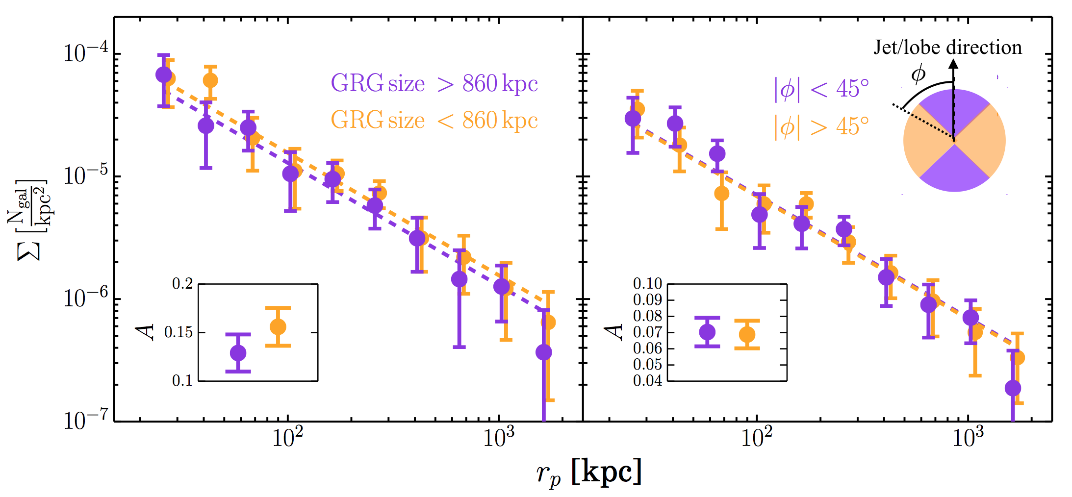
We now explore the radial distribution of satellite galaxies as a function of GRG size, i.e., the projected distance between two radio lobes. We separate the GRG sample into two equal number sub-samples according to their sizes. The corresponding median value of the GRG sizes is about 860 kpc. The left panel of Figure 6 shows the distribution of satellites around GRGs with sizes larger than 860 kpc and smaller than 860 kpc. We find that the distribution of satellites does not correlate with the sizes of GRGs. In other words, the local galaxy environments do not play a role in the sizes of GRGs.

Figure 7: Alignment of host galaxies and radio lobes. Left: Angle difference $\Delta\theta$ between the minor axes of the host galaxies and the jet/lobe directions with small (large) values indicating that jets/lobes tend be found along the minor (major) axes of the host galaxies. Right: Radial distribution of satellites as a function of angle difference. The distribution includes satellite galaxies with $M_{*}>10^{10.3}\,M_{\odot}$ and GRGs at $0.1<z<0.7$. The purple and orange data points indicate systems with $\Delta\theta<30^{\circ}$ and $\Delta\theta>30^{\circ}$ respectively. The best-fit A parameter values are shown in the inset.

Additionally to the sizes of GRGs, we also measure the satellite distribution as a function of the azimuthal angle of galaxy locations relative to the radio lobe directions. The azimuthal angle, $\phi$, defined as the angle between the location of a galaxy and the axis of radio lobes, is illustrated by the cartoon in the right panel of Figure 6. We have measured the radio lobe axes of GRGs manually. The right panel of Figure 6 shows the radial distribution of satellites for two azimuthal angle bins with $|\phi|<45^{\circ}$ for galaxies located towards the lobe directions and $|\phi|>45^{\circ}$ for galaxies located perpendicular to the lobe directions. Again, the two measurements are consistent with each other. This result demonstrates that the radio lobes of GRGs do not occur in preferential directions relative to the local galaxy environments.

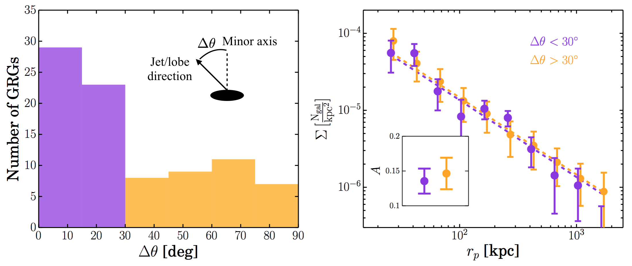
Finally, we measure the alignments between the radio lobes and the minor axis of the host galaxies. To do so, we (1) select host galaxies only with morphology best fitted by de Vaucouleurs’ profiles, i.e., elliptical galaxies, characterized by the Tractor algorithm (Lang et al., 2016), (2) use the shape measurements to obtain the position angles, and (3) compare the position angles of the minor axes of galaxies with the radio lobe directions. The left panel of Figure 7 shows the distribution of angle differences with $\Delta\theta=0^{\circ}$ indicating that the radio lobe direction is the same as the direction of host galaxy minor axis and $\Delta\theta=90^{\circ}$ indicating that the two are completely perpendicular to each other. The cartoon in the panel illustrates $\Delta\theta$.

We find that $>50\%$ of GRGs have radio jet/lobe directions within $30^{\circ}$ of the minor axes of the host galaxies. This distribution is $\sim 3\sigma$ (p-value $\simeq 0.004$) away from a random distribution based on K-S test for two samples, suggesting that a majority of the radio jets and lobes of GRGs preferentially escapes along the minor axes of their host galaxies. This trend is consistent with normal elliptical galaxies with extended radio emission as shown in Battye & Browne (2009). The right panel of Figure 7 shows the satellite distributions of the two GRG sub-samples with one having $\Delta\theta<30^{\circ}$ and the other having $\Delta\theta>30^{\circ}$. No correlation between the alignments of radio lobes and the axes of host galaxies and the satellite properties is detected.

Figure 8: Left: Illustration of the filament structures. The blue data point is a GRG and the grey data points are the random positions of the filament structure provided by Chen et al. (2016) catalog. The black data point indicates the nearest random point on the filament to the GRG. Right: Median distances between GRGs (blue), the optical control sample (red), the radio control sample (green) and random positions (grey) to the nearest filament structures.

3.3 The large-scale environments of GRGs

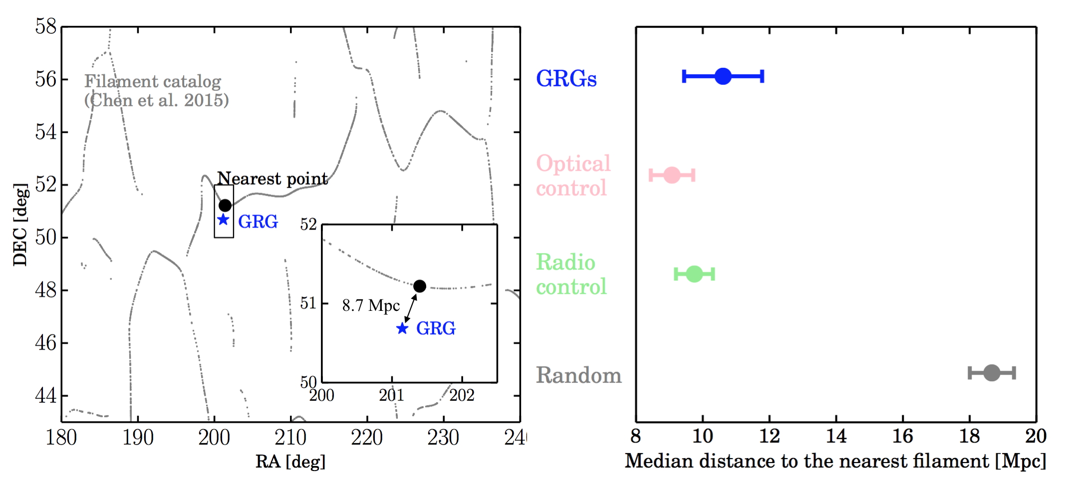
We now address the large-scale environments of GRGs. To do so, we measure the distance between each GRG and its nearest filamentary structure from the filament catalog (Chen et al., 2016). The left panel of Figure 8 shows an example. The blue data point shows a GRG and the grey points are the random sampling from the filaments with the redshift interval being closest to the redshift of the GRG. The black data point indicates the nearest random point from the filament. The projected physical distance between the GRG and the nearest random point is estimated. We perform this estimation for all the GRGs at $z<0.7$ and calculate the median distance of all the GRGs to the nearest filaments. We note that this value should not be considered as the intrinsic distance between the two entities given that the distance is based on the nearest random points on the filaments. Nevertheless, this measurement is sufficient for our purpose to make comparison between the distances of GRGs and the control samples to the nearest filaments.

The right panel of Figure 8 shows the result. We find that the median distance of GRGs to the nearest filaments is approximately 10 Mpc (blue), which is consistent with the same measurements of the two control samples as shown by the red and green data points. We also perform the same calculation using random points in the footprint with the result indicated by the grey data point. As can be seen, GRGs and the control samples are significantly closer to the nearby large-scale structures than random positions, illustrating that the estimator is sensible. The consistency between the measurements of GRGs and the control samples suggests that GRGs do not preferentially live in lower density environments relative to galaxies with similar optical properties.

4 Discussion

4.1 Comparison with previous studies

We have shown that the local and large-scale environments of GRGs are consistent with that of the control samples. This finding indicates that environments play a minor role (if any) on the physical processes giving rise to the origins of GRGs. This result is consistent with some previous results. For example, Komberg & Pashchenko (2009) performed a similar analysis with $\sim 20$ GRGs at $z<0.1$ and found that the local galaxy density of GRGs is similar to the galaxy density around normal radio galaxies. A recent analysis by Dabhade et al. (2020b) also shows that some GRGs are located in galaxy clusters, disfavoring the low-density environment hypothesis. In addition, if the IGM density plays a role in confining the sizes of GRGs, one would expect the sizes of GRGs evolve with redshift. However, such a trend is not observed (e.g., Machalski & Jamrozy, 2006; Kuźmicz et al., 2018), supporting the same picture that environments are not the primary factor for the sizes of GRGs.

On the other hand, some previous studies show different results. For instance, Malarecki et al. (2015) argue that there is a correlation between GRGs and their surrounding environments in contrast to our findings. Chen et al. (2011) also show that satellite galaxies around a GRG tend to be found in the direction of radio lobes, suggesting a correlation between radio jet/lobe directions and the galaxy distribution. This finding is in contrary to our results as shown in Figure 6. We note that sample variance could be one possible explanation for the inconsistency given that these studies are based on relative small samples. Future, larger GRG catalogs will be used to confirm our results.

4.2 The origins of GRGs

Our results suggest that environments are not the main driver for the enormous sizes of GRGs. This indirectly supports the scenario that such a radio structure is driven by the internal properties of the radio jet activity. One possible scenario is that GRGs are formed with a long lifetime of radio activity as suggested by some previous studies. For example, Hardcastle (2018) shows that with a fixed gas density environment, the sizes of radio galaxies depend on the lifetime of radio activity. Using the model from Hardcastle (2018), Hardcastle et al. (2019) further show that the sizes and power of observed radio galaxies, including GRGs, can be reproduced. Their results demonstrate that the sizes of radio lobes can reach to $\sim 1$ Mpc after a few hundred Myr of radio activity. While the model assumes a single phase of radio activity, it might not be realistic given that AGN activity can vary within much shorter timescales (e.g., Aranzana et al., 2018). This can be reconciled by the accumulation of multiple episodes of radio activity as indicated by previous studies (e.g., Bruni et al., 2020).

Figure 9: Fraction of blue satellite galaxies with $M_{*}>10^{10.3}\,M_{\odot}$ around GRGs (blue) and the two control samples (red: optical, green: radio) with $0.1<z<0.7$. The inset shows the best-fit values of the blue fraction for the three samples at 100 kpc. No significant correlation between the fraction of blue galaxies and the radio properties is observed.

4.3 The effects of radio feedback on the properties of surrounding galaxies

While we have primarily focused on addressing the mechanisms giving rise to the enormous sizes of GRGs, we can ask the following question in the context of radio feedback - do the current radio jets of GRGs influence the satellite galaxy properties? It has been observed, for example, that the power of radio jets is sufficient to remove hot gas within their trajectory and thereby create cavities of hot gas (e.g., Fabian, 2012). It is possible that such activity could also remove gas from satellite galaxies and quench those satellites. However, we emphasize that our measurements are only sensitive to the effects of the current radio jets on the properties of galaxies. Episodic radio activity and the corresponding feedback processes can impact the properties of galaxies on a longer timescale that is not reflected in our measurements.

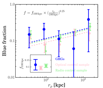
To explore radio mode feedback on quenching satellite galaxies, we first measure the fraction of blue satellite galaxies around GRGs and the two control samples. The blue satellite galaxies are selected with three observed colors, $g-z<1.7$, $g-z<2.1$, and $g-z<2.6$, for three redshift ranges $0.1<z<0.3$, $0.3<z<0.5$, and $0.5<z<0.7$ respectively. These observed color cuts are chosen to optimally separate blue and red galaxy populations based on the galaxy catalog from the PRIMUS survey (Coil et al., 2011; Cool et al., 2013).

Figure 9 shows the fraction of blue satellites around GRGs and the two control samples. We find that the blue fraction around GRGs is consistent with that around the two control samples. Furthermore, in all three samples the blue fraction increases with impact parameter from $\sim 10\%$ at 100 kpc to $\sim 30\%$ at 2 Mpc, consistent with trends observed in galaxy groups and clusters (e.g., Hansen et al., 2009). We characterize this trend with $f=f_{100\,kpc}\times\rm(r_{p}/100\,kpc)^{0.25}$ with the power index 0.25 being the best-fit value for the three measurements. The best-fit fraction at 100 kpc ($f_{100\,kpc})$ is shown in the inset of the figure. This result indicates that GRGs do not preferentially have more passive satellite galaxies despite their very large radio structures.

We also explore the effect of the current radio activity on galaxy properties by comparing the number of blue satellites as a function of GRG size and the galaxy location with respect to the radio lobes. We find that the number of blue galaxies depend on neither the sizes of GRGs nor the locations of galaxies relative to the radio lobes.

These results demonstrate that there is no apparent correlation between the properties of satellite galaxies and the presence of the giant radio structures, implying that the current radio jets do not greatly influence satellite properties. This result is consistent with the result of Pace & Salim (2014) who investigate the effect of typical radio AGNs on their surrounding galaxies. However, Shabala et al. (2011) show a different result. They find that galaxies located in the radio lobes of FRII-type galaxies are redder than galaxies outside of the radio lobes, offering evidence that radio jets quench star-formation in satellite galaxies. However, we note that Shabala et al. (2011) only considered galaxies located within radio lobes which consist of $\sim 1\%$ of all the satellite galaxies around FRII galaxies in their sample. In our analysis, we consider the bulk of satellite galaxies which may explain the apparent disagreement between the two results. We note that with the new LoTSS dataset, one can perform the same analysis as applied in Shabala et al. (2011). Nonetheless, such an analysis is beyond the scope of this paper.

5 Summary

We investigated the local and large-scale environments of GRGs by measuring the galaxy density around GRGs and their relative locations to the nearby large-scale structures. These measurements were derived from by cross-correlating a large GRG sample detected from LoTSS, with photometric galaxies from the DESI Legacy Surveys and a filament catalog obtained from the SDSS. Our main findings are summarized as follows:

1. We find that the properties of satellite galaxies, including number counts, magnitude and stellar mass distributions, and radial distribution, around GRGs from 20 kpc to 2 Mpc are consistent with the properties of satellite galaxies around the control samples. This result suggests that the local environments of GRGs mostly depend on the optical properties of the host galaxies.

2. We further explore the properties of satellites as a function of GRG properties and find that there is no correlation between the satellite properties and the sizes of GRGs as well as the locations of satellites relative to the radio jets/lobes.

3. We estimate the locations of GRGs with respect to the nearby large-scale filament structures and find that the median distance between GRGs and the nearest filaments is consistent with the median distances between the control samples and the nearest filaments. This result indicates that GRGs do not reside in low density environments in the context of large-scale structure.

These results indicate that the local and large-scale environments of GRGs are mostly determined by processes within the host galaxies. No significant correlation between the existence of giant radio structures and their surrounding environments traced by stars is found. These findings suggest that the environments of GRGs play little role in the mechanisms giving rise to the giant radio structures. In other words, our results disfavor the hypothesis that the formation of GRGs is related to their local environments (e.g., Mack et al., 1998).

In the context of feedback, we explore the effect of the current radio activity on the properties of satellite galaxies. We find that the number of blue satellites does not depend on the sizes of GRGs nor their relative locations with respect to the radio lobes. In addition, the fraction of blue satellite galaxies around GRGs is consistent with the fraction around the control samples. These findings illustrate that the current radio activity has minimal influence on the properties of the surrounding galaxies.

In the near future, the complete LoTSS survey will detect $\sim 12,000$ GRGs across half of the sky (Dabhade et al., 2020b). The combination of this large GRG sample, optical sky survey datasets, such as DESI (Levi et al., 2013), Euclid (Amiaux et al., 2012), and LSST (Ivezić et al., 2019), and X-ray sky survey datasets, such as eROSITA (Merloni et al., 2012) will enable much more precise characterizations of the properties of the GRG host galaxies, the surrounding environments of GRGs, and the corresponding redshift evolution. In addition to giant radio galaxies, there are giant radio sources hosted by quasars found from the local Universe to beyond redshift 2. An interesting research direction is to perform IFU observations for these high-redshift giant radio quasars to map out the distribution of diffuse cool gas via Lyman alpha emission - a different tracer for the environments of high-redshift giant radio quasars (e.g., Cantalupo et al., 2014). By doing so, we will shed new light on our understanding of not only the nature and origin of these giant radio structures but also the role they play in galaxy formation and evolution.

6 Data availability

The data underlying this article will be available at https://people.ucsc.edu/~tlan3/research/GRGs/.

References

- Abolfathi et al. (2018) Abolfathi, B., Aguado, D. S., Aguilar, G., et al. 2018, ApJS, 235, 42
- Alexander & Hickox (2012) Alexander, D. M. & Hickox, R. C. 2012, New A Rev., 56, 93
- Amiaux et al. (2012) Amiaux, J., Scaramella, R., Mellier, Y., et al. 2012, Proc. SPIE, 8442, 84420Z
- Aranzana et al. (2018) Aranzana, E., Körding, E., Uttley, P., et al. 2018, MNRAS, 476, 2501
- Battye & Browne (2009) Battye, R. A. & Browne, I. W. A. 2009, MNRAS, 399, 1888
- Benson et al. (2003) Benson, A. J., Bower, R. G., Frenk, C. S., et al. 2003, ApJ, 599, 38
- Best et al. (2005) Best, P. N., Kauffmann, G., Heckman, T. M., et al. 2005, MNRAS, 362, 25
- Best & Heckman (2012) Best, P. N. & Heckman, T. M. 2012, MNRAS, 421, 1569
- Boquien et al. (2019) Boquien, M., Burgarella, D., Roehlly, Y., et al. 2019, A&A, 622, A103
- Bower et al. (2008) Bower, R. G., McCarthy, I. G., & Benson, A. J. 2008, MNRAS, 390, 1399
- Bruni et al. (2020) Bruni, G., Panessa, F., Bassani, L., et al. 2020, MNRAS, 494, 902
- Bruzual & Charlot (2003) Bruzual, G., & Charlot, S. 2003, MNRAS, 344, 1000
- Cantalupo et al. (2014) Cantalupo, S., Arrigoni-Battaia, F., Prochaska, J. X., et al. 2014, Nature, 506, 63
- Chabrier (2003) Chabrier, G. 2003, PASP, 115, 763
- Chen et al. (2015) Chen, Y.-C., Ho, S., Freeman, P. E., et al. 2015, MNRAS, 454, 1140
- Chen et al. (2016) Chen, Y.-C., Ho, S., Brinkmann, J., et al. 2016, MNRAS, 461, 3896
- Chen et al. (2011) Chen, R., Peng, B., Strom, R. G., et al. 2011, A&A, 529, A5
- Chen et al. (2019) Chen, Y.-H., Heinz, S., & Enßlin, T. A. 2019, MNRAS, 489, 1939
- Coil et al. (2011) Coil, A. L., Blanton, M. R., Burles, S. M., et al. 2011, ApJ, 741, 8
- Cool et al. (2013) Cool, R. J., Moustakas, J., Blanton, M. R., et al. 2013, ApJ, 767, 118
- Condon et al. (1998) Condon, J. J., Cotton, W. D., Greisen, E. W., et al. 1998, AJ, 115, 1693
- Dabhade et al. (2017) Dabhade, P., Gaikwad, M., Bagchi, J., et al. 2017, MNRAS, 469, 2886
- Dabhade et al. (2020a) Dabhade, P., Mahato, M., Bagchi, J., et al. 2020, arXiv:2005.03708
- Dabhade et al. (2020b) Dabhade, P., Röttgering, H. J. A., Bagchi, J., et al. 2020, A&A, 635, A5
- Davé et al. (2019) Davé, R., Anglés-Alcázar, D., Narayanan, D., et al. 2019, MNRAS, 486, 2827
- Dey et al. (2019) Dey, A., Schlegel, D. J., Lang, D., et al. 2019, AJ, 157, 168
- Donoso et al. (2010) Donoso, E., Li, C., Kauffmann, G., et al. 2010, MNRAS, 407, 1078
- Duncan et al. (2019) Duncan, K. J., Sabater, J., Röttgering, H. J. A., et al. 2019, A&A, 622, A3
- Fabian (2012) Fabian, A. C. 2012, ARA&A, 50, 455
- Fanaroff & Riley (1974) Fanaroff, B. L. & Riley, J. M. 1974, MNRAS, 167, 31P
- Gopal-Krishna et al. (1989) Gopal-Krishna, Wiita, P. J., & Saripalli, L. 1989, MNRAS, 239, 173
- Hansen et al. (2009) Hansen, S. M., Sheldon, E. S., Wechsler, R. H., et al. 2009, ApJ, 699, 1333
- Hardcastle (2018) Hardcastle, M. J. 2018, MNRAS, 475, 2768
- Hardcastle et al. (2019) Hardcastle, M. J., Williams, W. L., Best, P. N., et al. 2019, A&A, 622, A12
- Hardcastle & Croston (2020) Hardcastle, M. J. & Croston, J. H. 2020, arXiv:2003.06137
- Ishwara-Chandra & Saikia (1999) Ishwara-Chandra, C. H. & Saikia, D. J. 1999, MNRAS, 309, 100
- Ivezić et al. (2019) Ivezić, Ž., Kahn, S. M., Tyson, J. A., et al. 2019, ApJ, 873, 111
- Komberg & Pashchenko (2009) Komberg, B. V. & Pashchenko, I. N. 2009, Astronomy Reports, 53, 1086
- Kuźmicz et al. (2018) Kuźmicz, A., Jamrozy, M., Bronarska, K., et al. 2018, ApJS, 238, 9
- Lan et al. (2014) Lan, T.-W., Ménard, B., & Zhu, G. 2014, ApJ, 795, 31
- Lan et al. (2016) Lan, T.-W., Ménard, B., & Mo, H. 2016, MNRAS, 459, 3998
- Lan (2020) Lan, T.-W. 2020, ApJ, 897, 97
- Lang et al. (2016) Lang, D., Hogg, D. W., & Mykytyn, D. 2016, The Tractor: Probabilistic astronomical source detection and measurement, ascl:1604.008
- Levi et al. (2013) Levi, M., Bebek, C., Beers, T., et al. 2013, arXiv:1308.0847
- Lin et al. (2004) Lin, Y.-T., Mohr, J. J., & Stanford, S. A. 2004, ApJ, 610, 745
- Lin et al. (2010) Lin, Y.-T., Shen, Y., Strauss, M. A., et al. 2010, ApJ, 723, 1119
- Machalski & Jamrozy (2006) Machalski, J. & Jamrozy, M. 2006, A&A, 454, 95
- Mack et al. (1998) Mack, K.-H., Klein, U., O’Dea, C. P., et al. 1998, A&A, 329, 431
- Malarecki et al. (2015) Malarecki, J. M., Jones, D. H., Saripalli, L., et al. 2015, MNRAS, 449, 955
- McNamara & Nulsen (2012) McNamara, B. R. & Nulsen, P. E. J. 2012, New Journal of Physics, 14, 055023
- Mendez et al. (2016) Mendez, A. J., Coil, A. L., Aird, J., et al. 2016, ApJ, 821, 55
- Merloni et al. (2012) Merloni, A., Predehl, P., Becker, W., et al. 2012, arXiv:1209.3114
- Mandelbaum et al. (2009) Mandelbaum, R., Li, C., Kauffmann, G., et al. 2009, MNRAS, 393, 377
- More et al. (2016) More, S., Miyatake, H., Takada, M., et al. 2016, ApJ, 825, 39
- Nelson et al. (2019) Nelson, D., Pillepich, A., Springel, V., et al. 2019, MNRAS, 490, 3234
- Pace & Salim (2014) Pace, C. & Salim, S. 2014, ApJ, 785, 66
- Saripalli et al. (1986) Saripalli, L., Gopal-Krishna, Reich, W., et al. 1986, A&A, 170, 20
- Schaye et al. (2015) Schaye, J., Crain, R. A., Bower, R. G., et al. 2015, MNRAS, 446, 521
- Shabala et al. (2011) Shabala, S. S., Kaviraj, S., & Silk, J. 2011, MNRAS, 413, 2815
- Shimwell et al. (2019) Shimwell, T. W., Tasse, C., Hardcastle, M. J., et al. 2019, A&A, 622, A1
- Silk & Rees (1998) Silk, J. & Rees, M. J. 1998, A&A, 331, L1
- Subrahmanyan et al. (1996) Subrahmanyan, R., Saripalli, L., & Hunstead, R. W. 1996, MNRAS, 279, 257
- Tinker et al. (2017) Tinker, J. L., Brownstein, J. R., Guo, H., et al. 2017, ApJ, 839, 121
- Tinker et al. (2019) Tinker, J. L., Cao, J., Alpaslan, M., et al. 2019, arXiv e-prints, arXiv:1911.04507
- Williams et al. (2019) Williams, W. L., Hardcastle, M. J., Best, P. N., et al. 2019, A&A, 622, A2
- Willis et al. (1974) Willis, A. G., Strom, R. G., & Wilson, A. S. 1974, Nature, 250, 625
- Worrall (2009) Worrall, D. M. 2009, A&A Rev., 17, 1
- Wright et al. (2010) Wright, E. L., Eisenhardt, P. R. M., Mainzer, A. K., et al. 2010, AJ, 140, 1868
- Yang et al. (2018) Yang, G., Brandt, W. N., Darvish, B., et al. 2018, MNRAS, 480, 1022
- York et al. (2000) York, D. G., Adelman, J., Anderson, J. E., et al. 2000, AJ, 120, 1579