The intrinsic reddening of the Magellanic Clouds as traced by background galaxies – II. The Small Magellanic Cloud

Abstract

We present a map of the total intrinsic reddening across $\simeq$ 34 deg² of the Small Magellanic Cloud (SMC) derived using optical ($ugriz$) and near-infrared (IR; $YJK_{\mathrm{s}}$) spectral energy distributions (SEDs) of background galaxies. The reddening map is created using a subsample of 29,274 galaxies with low levels of intrinsic reddening based on the lephare $\chi^{2}$ minimisation SED-fitting routine. We find statistically significant enhanced levels of reddening associated with the main body of the SMC compared with regions in the outskirts [$\Delta E(B-V)\simeq 0.3$ mag]. A comparison with literature reddening maps of the SMC shows that, after correcting for differences in the volume of the SMC sampled, there is good agreement between our results and maps created using young stars. In contrast, we find significant discrepancies between our results and maps created using old stars or based on longer wavelength far-IR dust emission that could stem from biased samples in the former and uncertainties in the far-IR emissivity and the optical properties of the dust grains in the latter. This study represents one of the first large-scale categorisations of extragalactic sources behind the SMC and as such we provide the lephare outputs for our full sample of $\sim$ 500,000 sources.

1 Introduction

The dust content of galaxies, and specifically the effects this has on photometric observations, is of great importance in the field of galaxy formation and evolution. Within this framework, the Magellanic Clouds (MCs) are arguably two of the most studied galaxies, due primarily to their close proximity ($\sim 50-60$ kpc) and wealth of different stellar populations spanning all ages. The MCs are benchmark laboratories for studies of, amongst others, star formation at lower ($0.2-0.5$ Z_⊙) metallicities (e.g. Gouliermis, Hony, & Klessen, 2014; Zivkov et al., 2018), constraining the extragalactic distance scale (and by extension the Hubble constant $H_{0}$, e.g. de Grijs, Wicker, & Bono, 2014; de Grijs & Bono, 2015; Riess et al., 2019; Freedman et al., 2020), as well as the metallicity dependence of the period–luminosity relation of variable stars (see e.g. Gieren et al., 2018; Groenewegen, 2018; Muraveva et al., 2018; Ripepi et al., 2019). All such studies are dependent upon an understanding of the amount and spatial distribution of dust across the MCs, however the issue is that the use of differently aged stellar populations to quantify the reddening in the MCs results in statistically significant differences (this is further complicated by variations in metallicity, three-dimensional distributions of the stars and dust, etc.). For example, the use of young stellar populations (e.g. young star clusters and Cepheids, Nayak et al., 2018; Joshi & Panchal, 2019) results in reddening maps with enhanced levels of reddening associated with regions that are actively forming stars and lower levels of reddening in more quiescent regions. In contrast, reddening maps based on older stars [e.g. red clump (RC) and RR Lyrae] imply systematically lower levels and/or negligible homogeneously distributed levels of reddening (see e.g. Zaritsky et al., 2002; Muraveva et al., 2018; Górski et al., 2020). Although these differences can be small, it is worth stressing that even a modest change in $\Delta E(B-V)$, such as the difference between the RC reddening maps of Haschke, Grebel, & Duffau (2011) and Górski et al. (2020) of $\Delta E(B-V)=0.06$ mag, can have significant implications. Even though both maps use the same data from the third phase of the Optical Gravitational Lensing Experiment (OGLE-III; Udalski, 2003) as an input, the difference between their determined reddening values affects the inferred value for the Hubble constant at greater than the 3 km s^-1 Mpc^-1 level (see e.g. section 3.1 of Riess et al., 2009) and as well as the three-dimensional structure inferred from the use of resolved stars (e.g. Ripepi et al., 2017; Choi et al., 2018).

In Bell et al. (2019, hereafter Paper I) we introduced a technique to map the intrinsic reddening of a foreground extinguishing medium using the spectral energy distributions (SEDs) of background galaxies. This technique not only removes the aforementioned stellar population dependency on the derived reddening values, but also probes the total reddening by sampling the full column depth of the extinguishing medium. We piloted this method on two 1.77 deg² regions in the Small Magellanic Cloud (SMC) – the main body and the southern outskirts – and demonstrated that when using galaxies with low intrinsic reddening one can clearly see signs of higher intrinsic reddening associated with the main body compared with the more quiescent outskirts. In this study, we extend this pilot study to map the total intrinsic reddening across the $\simeq$ 34 deg² of the SMC covered by the combined footprints of the Survey of the MAgellanic Stellar History (SMASH; Nidever et al., 2017) and the Visible and Infrared Survey Telescope for Astronomy (VISTA) survey of the Magellanic Clouds system (VMC; Cioni et al., 2011).

The structure of this paper is as follows. In Section 2 we describe the processes involved in creating and fitting the SEDs of background galaxies as well as provide a comparison of the results of the SED fitting with other extragalactic studies. The details of how we create our intrinsic reddening map of the SMC is presented in Section 3. We discuss our reddening map and compare it with literature reddening maps of the SMC based on different tracers in Section 4, and summarise our findings in Section 5.

2 Creating and fitting SEDs of galaxies

2.1 Creating the SEDs

Our data set consists of optical $ugriz$ and near-infrared (IR) $YJK_{\rm{s}}$ photometry taken as part of the SMASH and VMC surveys, respectively, that cover the wavelength range 0.3–2.5 $\mu$m. Paper I describes in detail the processes involved in selecting likely background galaxies on which to perform photometry. To briefly summarise, we use the VMC point-spread function (PSF) photometric catalogues (Rubele et al., 2015, 2018) and retain those sources that satisfy the following colour–magnitude and morphological selections: $J-K_{\rm{s}}>1.0$ mag, $K_{\rm{s}}>15$ mag, an associated stellar probability of less than 0.33 and a $K_{\rm{s}}$-band sharpness index of greater than 0.5 (see Paper I for details regarding both the stellar probability and sharpness index).

Fluxes for each of our targets are measured using the Lambda Adaptive Multi-Band Deblending Algorithm in R (lambdar, v0.20.5; Wright et al. 2016). The reader is directed to Paper I for a full discussion regarding the measurement of fluxes in addition to the calibration of both the optical and near-IR data sets onto an AB magnitude system. We adopt the fluxes measured using a default circular aperture of diameter 3 arcsec. Since Paper I, we have optimised the parameters used for per-exposure PSF estimation within lambdar, allowing for more accurate PSF estimation per observation. This subsequently allows for more accurate (missed-flux) aperture corrections for our standard aperture photometry (see Wright et al., 2016 for details) per observation, and more reliable photometry overall. The final flux measurement for a given source is simply the weighted mean of all available measurements (including those in overlap regions) in that band and for which we set the weights equal to the inverse square of the corresponding uncertainty on the flux.

To ensure reliable fits to the SEDs, we only retain sources for which we measure positive fluxes in at least four of the eight available bands. Finally, we account for foreground Milky Way (MW) reddening by de-reddening the individual fluxes by an amount equivalent to $E(B-V)=0.034$ mag. This foreground subtraction is an average correction to the fluxes as small-scale structures will cause variations across the survey area (see section 2.5 of Paper I and Bailey et al., 2015 for details). The resulting catalogue contains a total of 497,577 sources (hereafter referred to as the full SMC sample) distributed across $\simeq$ 34 deg² (see Fig. 1). Note that the strange tile shape in the south-eastern VMC coverage is due to the presence of a Bridge tile that we do not include in this work as we will study the reddening of the Magellanic Bridge in a future work.

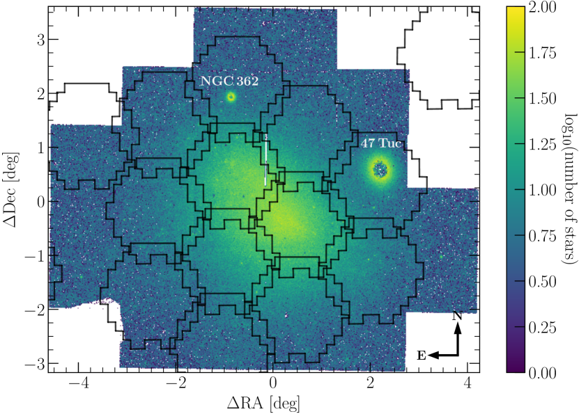
Figure 1: Stellar density plot of the SMC as observed by the VMC survey. The origin of the plot corresponds to the centre of the SMC as given by the HYPERLEDA catalogue of Paturel et al. (2003). The black hexagons denote the positions of the SMASH fields. The combined SMASH-VMC footprint is $\simeq$ 34 deg². The positions of the prominent foreground Milky Way globular clusters 47 Tucanae and NGC 362 are also shown. The vertical stripe at $\Delta$RA $\simeq-0.2$ deg is due to a narrow gap in the VMC observations that is currently being filled.

2.2 Fitting the SEDs

Paper I provides a comprehensive discussion of the processes involved in fitting the SEDs of background galaxies, including the choice of SED-fitting code, templates, redshift prior and attenuation curve, so we refer the reader to that description for particulars.

Briefly, we adopt the lephare SED-fitting code that allows one to fit several suites of templates – both theoretical and empirical – including galaxies, quasi-stellar objects (QSOs) and stars to determine which provides the best fit to the data based on a simple $\chi^{2}$-minimisation routine. In Paper I we performed the SED fits using both the theoretical and empirical galaxy templates to study the effects of template-dependency on the resulting best-fitting reddening values. We found that the use of theoretical templates (in that case the so-called COSMOS templates included as part of the lephare code) resulted in enhanced levels of reddening at the $\Delta E(B-V)$ $\simeq$ 0.2 mag level compared to the reddening values inferred from the SED fits using the empirical (AVEROI_NEW) templates. After comparing the reddening maps inferred from background galaxies with those available in the literature, based on various stellar components in the MCs, it was hard to reconcile these enhanced levels of reddening with the difference in the depth of the SMC sampled by different tracers, thus prompting us to prefer the reddening values based on the AVEROI_NEW templates.

In this study, we only adopt the empirical AVEROI_NEW galaxy templates, in addition to the QSO and stellar templates discussed in Paper I. The redshift prior we adopt is included as part of lephare and has been calibrated using the VIMOS VLT Deep Survey (VVDS; Le Fèvre et al., 2005). Finally, we adopt the attenuation curve resulting from the combined studies of Prevot et al. (1984) and Bouchet et al. (1985) that is included as part of the lephare code. As noted by Ilbert et al. (2009), there will inevitably be differences in the attenuation curve from one galaxy to the next, however the aforementioned curve is representative of the SMC attenuation curve and is also well suited for the six galaxy types (E, Sbc, Scd, Irr and two starburst galaxies) from which the AVEROI_NEW templates were created (see Paper I for details).

We run lephare on the standard aperture sample of galaxies allowing the redshift to vary from $z=0.0$ to 6.0 in steps of $\Delta z=0.02$. As discussed in Paper I, the intervening dust in the SMC provides an additional component of the line-of-sight reddening. We therefore allow additional reddening for all galaxy types, in contrast to the typical implementation for which additional reddening is only permitted for galaxy templates of type Sc and bluer/later (see e.g. Arnouts et al., 2007). This allows us to use galaxies with spectral types of Sb and redder/earlier as direct probes of the intrinsic reddening of the SMC. To limit degeneracies in the best-fitting solutions, we allow the reddening to vary for the galaxy and QSO templates from $E(B-V)=0.0$ to 0.5 mag in steps of $\Delta E(B-V)=0.05$ mag. Table 1 provides the lephare outputs, including photometric redshift, galaxy type, best-fitting reddening values, etc. for the 497,577 sources in the full SMC sample and Table 2 provides the numbers of sources classified as galaxies, QSOs and stars based on the associated minimum $\chi^{2}$ value of the best-fitting template.

Table 1: A sample of the lephare output for the 497,577 sources in the full SMC sample. We only show the ID, RA and Dec. (J2000.0), the best-fitting photometric redshift with associated $1\sigma$ limits, the maximum likelihood photometric redshift with associated $1\sigma$ limits, the best-fitting galaxy/QSO template and the associated $\chi^{2}$ value for the best-fitting galaxy/QSO template as a representation of its content. The full table (available as Supporting Information in the online version of the paper) also includes the best-fitting $E(B-V)$ value, the best-fitting distance modulus, the number of photometric bands in the SED, the combination of photometric bands in the SED (termed “Context” in lephare; see Notes below), the best-fitting stellar template and the associated $\chi^{2}$ value for the best-fitting stellar template.

ID	RA (J2000.0)	Dec. (J2000.0)	$z_{\rm{BEST}}$	$z_{\rm{BEST}}^{-1\sigma}$	$z_{\rm{BEST}}^{+1\sigma}$	$z_{\rm{ML}}$	$z_{\rm{ML}}^{-1\sigma}$	$z_{\rm{ML}}^{+1\sigma}$	Template${}_{\rm{G/Q}}^{a}$	$\chi^{2}_{\rm{G/Q}}$
	deg	deg
1	8.22274	$-75.59664$	1.0984	1.0463	1.1526	0.6316	0.5288	1.1082	3	0.1229
2	8.23561	$-75.53493$	1.0176	0.1028	2.0265	0.6598	0.1635	1.1510	72	0.1256
3	8.24278	$-75.51370$	1.0178	0.0547	1.0429	0.0773	0.0309	0.1376	3	3.2894
4	8.17035	$-75.51329$	0.3901	0.3798	0.4001	–99.0	–99.0	–99.0	4	2064.5100
5	8.16404	$-75.51295$	1.0671	1.0416	1.1145	0.7988	0.3493	1.0796	6	0.7664
6	8.17099	$-75.51268$	1.0634	0.5162	1.0801	0.7641	0.5511	0.9438	71	0.4137
7	8.16723	$-75.51165$	1.0804	1.0607	1.1003	0.5580	0.5093	1.0875	4	14.5201
8	8.04942	$-75.50990$	1.0634	1.0513	1.0776	0.5704	0.4296	1.1121	4	5.2806
9	8.20849	$-75.50972$	0.5221	0.5114	0.5331	0.5234	0.5036	0.5448	2	12.5986
10	7.88062	$-75.50932$	0.1384	0.1189	0.1593	0.1418	0.1215	0.1618	48	19.8340

Notes: The reader is referred to the lephare documentation for more details regarding the outputs of the code as well as the various template libraries contained within.

^a Best-fitting galaxy/QSO templates are as follows: (1) Seyfert 1.8, (2) Seyfert 2, (3) QSO1, (4) BQSO1, (5) TQSO1, (6) QSO2, (7) Torus (QSO2), (8) Mrk 231, (9) IRAS 19254–7245, (10) NGC 6240, (11–31) E, (32–47) Sbc, (48–58) Scd, (59–68) Irr, (69–72) Starburst.

^b Context is a numerical representation in lephare specifying the combination of bands present in the input catalogue and is defined as $\sum_{i=1}^{i=N}2^{i-1}$, where $i$ is the band number (in our case $u=1$, $g=2$, …, $J=7$, and $K_{\rm{s}}=8$), and $N$ is the total number of bands.

Table 2: Number of sources classified as a galaxy, QSO or star by lephare. The values in parentheses denote the corresponding percentages of the total number of sources in the full SMC sample (see Section 2.2).

Galaxies	QSOs	Stars
190,310 (38.2)	271,556 (54.6)	35,711 (7.2)

2.3 Galaxy photometric redshift and spectral type distributions

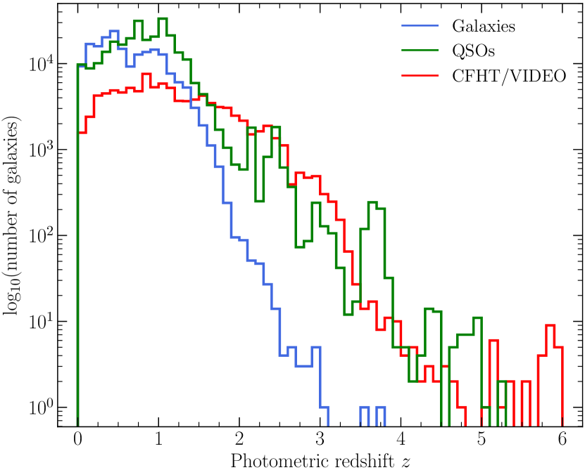
Figure 2: Photometric redshift distributions of sources classified by lephare as galaxies (blue) and QSOs (green) in the full SMC sample. For comparison, we also show the redshift distribution of galaxies in the CFHT/VIDEO (red) sample (see text for details).

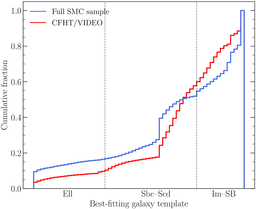
Figure 3: Normalized cumulative distributions showing the distribution of best-fitting galaxy templates (elliptical, spiral and irregular/starburst) in the full SMC (blue) and CFHT/VIDEO (red) samples.

Given that this study represents one of the first large-scale homogeneous cataloguing and categorisations of background galaxies behind the SMC, it is relevant to place these results in context by discussing some galaxy statistics. Figs. 2 and 3 show the photometric redshift and best-fitting galaxy template distributions, respectively, for the full SMC sample compared with those resulting from the analysis of the combined CFHTLS-DF1 $ugriz$ and VISTA Deep Extragalactic Observations (VIDEO) $ZYJHK_{\mathrm{s}}$ data performed by Jarvis et al. (2013).

We preferentially adopt the photometric redshift from the median of the maximum likelihood distribution (termed $z_{\mathrm{ML}}$ in lephare). When this is not available, however, we simply adopt the photometric redshift corresponding to the redshift with the minimum $\chi^{2}$ value (termed $z_{\mathrm{BEST}}$; see Section 3.5 of Ilbert et al., 2009 for details). Our reasoning for preferentially adopting $z_{\mathrm{ML}}$ is that, as discussed in Ilbert et al. (2013), whilst $z_{\mathrm{ML}}$ and $z_{\mathrm{BEST}}$ are broadly similar, the use of the median of the likelihood distribution results in more reliable uncertainties on the photometric redshift and also reduces the effect of aliasing in photometric redshift space. In Paper I we found clear evidence (see their figs. 10 and 11) of differences in the peak of the galaxy redshift distribution between the two regions studied (the outskirts and the south-western main body), that we attributed to the combined effects of crowding and incompleteness in the latter. For the full SMC sample, we calculate a median redshift of $z_{\mathrm{med}}=0.55$ and a median absolute deviation of $z_{\mathrm{MAD}}=0.44$. At higher redshifts, we see a steep decline with only three galaxies at redshifts greater than 3. In Fig. 2 we also show the QSO redshift distribution of the full SMC sample, which are those sources with a lower $\chi^{2}$ value for a QSO template than for a galaxy template. Given that, on average, we expect QSOs to be brighter than the quiescent background galaxy population, it is no surprise to see the QSO redshift distribution peak and extend to higher redshifts ($z_{\mathrm{med}}=0.84$; $\simeq$ 1000 sources with $z>3$). Comparing the galaxy redshift distribution of the full SMC sample with that of the CFHT/VIDEO sample, we see that the latter not only has a lower peak, but a broader distribution than that of the full SMC sample ($z_{\mathrm{med}}=1.06$; $z_{\mathrm{MAD}}=0.72$). This discrepancy can be attributed to the combination of differences in both the areal coverage and photometric sensitivity of the two samples. Whilst the CFHT/VIDEO photometry is much deeper than our combined SMASH-VMC photometry [with 5$\sigma$ magnitude limits $\gtrsim$ 1.5 mag (AB) across all eight bands], it only covers an area of 1 deg² on the sky compared to the $\simeq$ 34 deg² covered by our sample. As regards the distribution of best-fitting galaxy templates, Fig. 3 shows that the distributions of the full SMC and CFHT/VIDEO samples are consistent at the 10–15 per cent level across all spectral types.

2.4 Comparison of photometric to spectroscopic redshifts

Figure 4: Histogram showing the differences between the spectroscopically determined redshifts of QSOs behind the SMC and the corresponding photometric redshifts calculated by lephare. The various statistics regarding the comparison of the two redshift determinations are discussed in the text.

Table 3: Comparison between the spectroscopically determined and calculated photometric redshifts for QSOs behind the SMC. The full table is available as Supporting Information in the online version of the paper.

Name	$z_{\mathrm{spec}}$	$z_{\mathrm{phot}}$	Ref.
XMMU J003917.7–730330	0.345	$0.400\pm 0.014$	1
MQS J004143.75–731017.1	0.217	$0.259^{+0.026}_{-0.029}$	2
2MASS J00414502–7254356	0.267	$0.518^{+0.015}_{-0.014}$	3
MQS J004152.35–735626.8	0.422	$0.289^{+0.065}_{-0.019}$	2
MQS J004336.54–735615.1	0.661	$0.279\pm 0.014$	2
MQS J004736.12-724538.2	0.572	$0.614^{+0.017}_{-0.014}$	3
OGLE SMC100.4 26477	0.288	$0.264^{+0.024}_{-0.022}$	3
MQS J005311.80-740852.6	0.293	$0.258^{+0.076}_{-0.089}$	2
XMMU J005325.9-714821	0.982	$0.881^{+0.014}_{-0.015}$	1
OGLE SMC105.7 34076	0.505	$0.500\pm 0.014$	3

Notes: ^a Associated 1$\sigma$ limits on $z_{\mathrm{BEST}}$ are unphysical (see footnote 4 in text).

References: (1) Maitra et al. (2019), (2) Kozłowski et al. (2013), (3) Kozłowski et al. (2011), (4) Public ESO Spectroscopic Survey of Transient Objects (PESSTO; Smartt et al., 2015).

To further test the validity of the lephare outputs we compare the calculated photometric redshifts to spectroscopically determined redshifts of QSOs behind the SMC. Our sample comprises 232 spectroscopically confirmed QSOs from Dobrzycki et al. (2003a, b), Geha et al. (2003), Véron-Cetty & Véron (2010), Kozłowski, Kochanek, & Udalski (2011), Kozłowski et al. (2013), Ivanov et al. (2016), and Maitra et al. (2019), for which we find 229 unique matches in the VMC PSF photometric catalogues covering the SMC within a 1 arcsec matching radius. Of the 229 QSOs, only 46 satisfy the colour–magnitude and morphological selections described in Section 2.1. Table 3 lists the comparison between the photometric redshifts calculated by lephare and the corresponding spectroscopically determined redshifts. Fig. 4 shows that the two redshift determinations agree, in general, very well with a median difference of $\Delta z=-0.006$ and median absolute deviation of $\Delta z=0.101$. Following Dahlen et al. (2013), we also report additional statistics including the bias, outlier fraction (OLF), full scatter ($\sigma_{F}$) and scatter having removed outliers ($\sigma_{O}$). Even though the sample from which these statistics are drawn is small, it is worth noting that they are all consistent with the statistics calculated by Dahlen et al. (2013) who tested several photometric redshift codes on a sample of $\sim$ 600 galaxies from the Cosmic Assembly Near-infrared Deep Extragalactic Legacy Survey (CANDELS) GOODS-S data (see their tables 2 and 3).

3 Determining the intrinsic reddening

In Paper I we introduced several effects that could potentially affect the inferred reddening values, including the number of bands used in the SED fit, blending and incompleteness at fainter magnitudes and redshift probability distributions (PDF$z$) with multiple peaks (see appendix A of Paper I for details). To briefly summarise, we retained only those sources for which fluxes in all eight bands are available, those sources that are brighter than the magnitude at which incompleteness starts to affect the sample and those sources that only have a single peak in the PDF$z$. We found that by imposing these constraints on the sample, the inferred reddening maps were not significantly affected. Although there were minor morphological differences, the median reddening across a tile was only affected at the $\Delta E(B-V)$ $\simeq$ 0.03 mag level. Note that the magnitude cut imposed as a result of decreasing completeness is performed on a VMC tile-by-tile basis. Imposing these constraints reduces our sample size from the 497,577 sources in the full SMC sample to 197,821 galaxies/QSOs in the cleaned SMC sample.

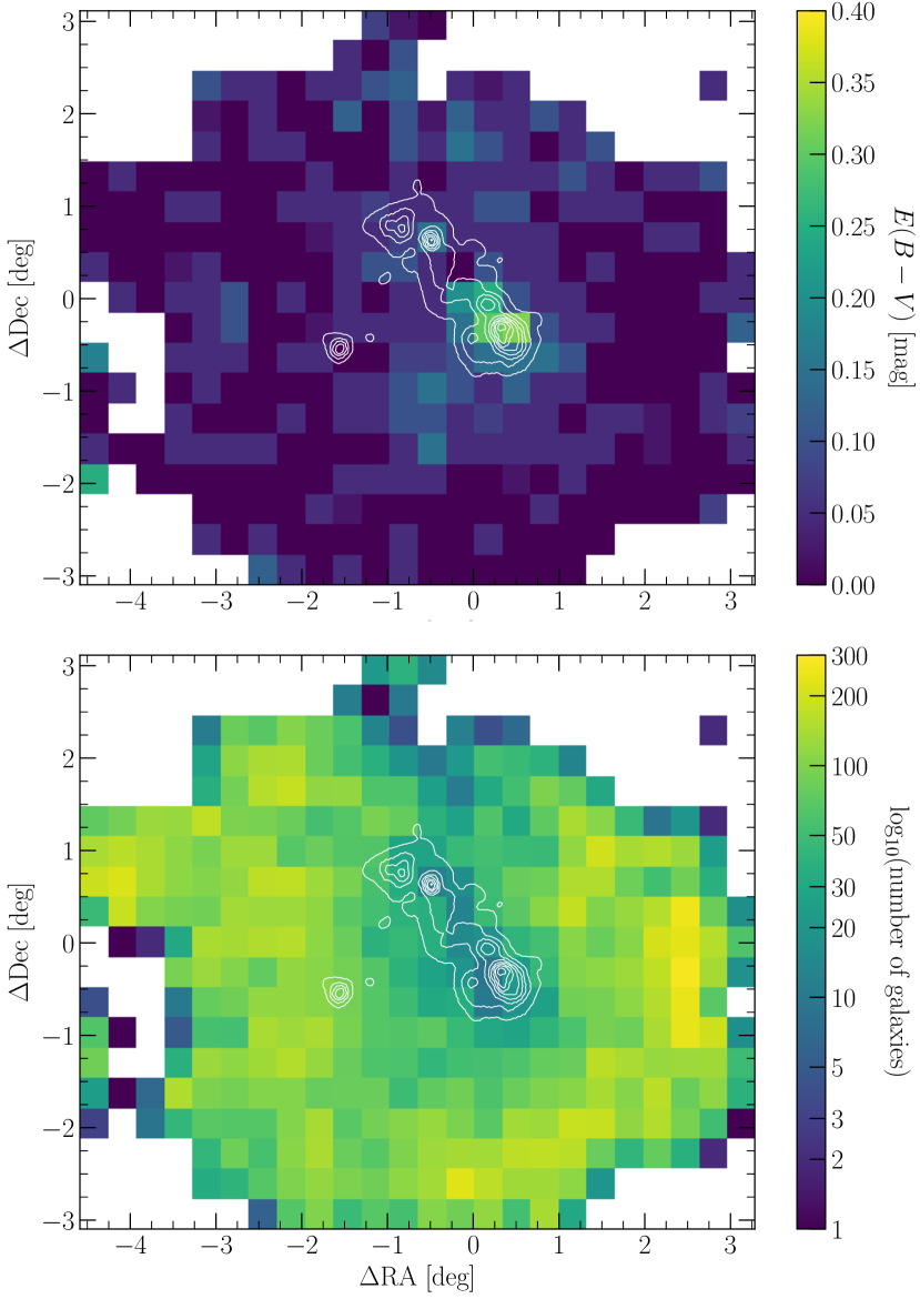
Figure 5: Top panel: $20\times 20$ arcmin² resolution reddening map of the combined SMASH-VMC footprint covering $\simeq$ 34 deg² of the SMC. This map has been created using only galaxies with spectral types of Sbc and redder/earlier according to the AVEROI_NEW templates and that satisfy the three criteria designed to refine the sample (see Section 2.2). Bottom panel: As the top panel, but showing the number density of galaxies used to create the reddening map. The contours in both panels represent the IRAS 100 $\mu$m dust emission.

Fig. 5 shows a $20\times 20$ arcmin² resolution reddening map covering $\simeq$ 34 deg² of the SMC. The $E(B-V)$ value associated with a given bin is simply the median value of all best-fitting $E(B-V)$ values. The total number of galaxies used to create the reddening map (with spectral types of Sb and redder/earlier from the cleaned SMC sample) is 29,274 distributed across 343 bins. Note that as demonstrated in Paper I (see also Section 2.2), reddening maps based on QSOs and/or all galaxies are inconsistent with the morphology of dust within the SMC, and thus we use only those galaxies with low levels of intrinsic reddening. The number of galaxies in a given bin ranges from 1 to 276, with a median of 82. There are 5 bins for which the associated $E(B-V)$ value is based on only a single galaxy. Several bins in the outskirts of the combined SMASH-VMC footprint contain only a few galaxies and these likely explain the enhanced levels of reddening associated with some outskirt bins. In the central regions of the SMC, that are affected by incompleteness due to crowding, we note that the number of galaxies per bin is significantly lower than the median value of 82 (see bottom panel of Fig. 5). However, in the regions of Fig. 5 traced by the IRAS 100 $\mu$m dust emission contours, we have at least 9 galaxies in all bins.

From Fig. 5 we can clearly see the enhanced levels of intrinsic reddening associated with the main body, and in particular the south-western regions. Whilst we detect increased levels of intrinsic reddening in some north-eastern regions of the main body, there is no clear continuous region of enhanced reddening along the length of the main body (as traced by the 100 $\mu$m emission). This pattern is remarkably similar to the 5780 and 5797 $\rm{\AA}$ diffuse interstellar band (DIB) maps produced by Bailey et al. (2015, see their fig. 7). Furthermore, we detect no clear signature of enhanced levels of intrinsic reddening, with respect to the low-level background, in the region associated with the Wing ($\Delta$RA$\,\simeq$ –1.5, $\Delta$Dec$\,\simeq$ –0.5 deg). In contrast, Fig. 5 shows small regions of enhanced levels of intrinsic reddening to both the north and south of the main body. These regions do not coincide with any known morphological features (see e.g. El Youssoufi et al., 2019), however the regions to the south do coincide with overabundances of Ca II K and Na I D₂ atomic absorption as measured by Bailey et al. (2015). The median intrinsic reddening across the combined SMASH-VMC footprint is $E(B-V)_{\mathrm{med}}=0.05$ mag, with a maximum value of $E(B-V)=0.33$ mag in the south-western region of the main body. The median uncertainty on the reddening within a given bin (calculated as the standard deviation of the best-fitting reddening values within a given bin) is $\sigma_{E(B-V)_{\mathrm{med}}}=0.10$ mag. For bins with only a single galaxy we assume an uncertainty of 0.05 mag based on the adopted spacing of $E(B-V)=0.05$ mag in the lephare fitting (see Section 3). Table 4 provides the median reddening values, standard deviations and the number of galaxies in each of the 343 bins covering the combined SMASH-VMC footprint of the SMC.

Table 4: Median reddening values, standard deviations and the number of galaxies in each of the 343 bins covering the combined SMASH-VMC footprint of the SMC. The full table is available as Supporting Information in the online version of the paper.

RA (J2000.0)	Dec. (J2000.0)	$E(B-V)_{\mathrm{med}}$	$\sigma_{E(B-V)}$	No. galaxies
deg	deg	mag	mag
$-2.45490$	$-2.93296$	0.125	0.144	6
$-2.12704$	$-2.93296$	0.050	0.096	66
$-1.79918$	$-2.93296$	0.000	0.085	101
$-1.47132$	$-2.93296$	0.050	0.087	49
$-1.14346$	$-2.93296$	0.000	0.119	68
$-0.81560$	$-2.93296$	0.050	0.085	56
$-0.48774$	$-2.93296$	0.000	0.105	107
$-0.15988$	$-2.93296$	0.000	0.080	88
0.16798	$-2.93296$	0.000	0.099	119
0.49584	$-2.93296$	0.000	0.101	55

4 Discussion and comparisons

In this study, we have presented a map of the total intrinsic reddening covering $\simeq$ 34 deg² of the SMC as defined by the combined SMASH-VMC footprint. Following Paper I, the use of background galaxies with low levels of intrinsic reddening allows us to observe clear signatures of enhanced levels of reddening associated with the main body of the SMC. However, we do not see such enhancements in either the northern region of the main body or the SMC Wing. In this section we will compare our reddening map with large-scale reddening maps of the SMC based on different tracers to highlight potential discrepancies with respect to both the line-of-sight reddening values and the distribution of dust across the galaxy. Note that in the figures presented below we do not apply any correction for the difference in the volume sampled between the reddening map based on background galaxies and those based on the stellar components of the SMC. Furthermore, if the literature maps include the contribution from the foreground MW, then we remove this component by simply subtracting $E(B-V)=0.034$ mag (see Section 2.1) from each reddening measurement. As a result of removing the MW component of the reddening, a small fraction of measurements in the literature maps become negative. We therefore exclude such measurements from our analysis, but note that their removal does not affect the conclusions of the comparisons below.

4.1 Literature SMC reddening maps

In Paper I we introduced several literature reddening maps based on various stellar components of the SMC. The discussion, however, was limited to only the two tiles investigated as part of that pilot study. In this study, we retain the reddening maps of Zaritsky et al. (2002, specifically that based on the cool stars), Muraveva et al. (2018), Rubele et al. (2018) and Tatton et al. (submitted), and refer the reader to Paper I for details concerning each of these. Additionally, we include as part of our comparison recent reddening maps produced by Joshi & Panchal (2019) and Górski et al. (2020) as well as the dust emission map based on far-IR and submillimetre observations taken as part of the HERschel Inventory of The Agents of Galaxy Evolution (HERITAGE) project (Meixner et al., 2013).

4.1.1 Joshi & Panchal (2019)

Joshi & Panchal (2019) used $V$- and $I$-band data from OGLE-IV (Udalski, Szymański, & Szymański, 2015) to create a $\simeq$ 5 deg² reddening map of the SMC using a combination of 4546 fundamental mode and first overtone mode Cepheids. The authors do not derive reddening values for individual Cepheids, but instead use period–luminosity relations to determine the reddening towards a given region containing a minimum of 10 Cepheids. In total, there are 136 regions that can be used to map the reddening across the SMC. To transform the derived $E(V-I)$ values into $E(B-V)$ we adopt the prescription of Cardelli, Clayton, & Mathis (1989) [$E(V-I)=1.32\times E(B-V)$].

4.1.2 Górski et al. (2020)

Górski et al. (2020) recently re-determined the reddening in the SMC using $V$- and $I$-band data from OGLE-III based on the colour of the RC. The data used are identical to those in Haschke et al. (2011), however Górski et al. (2020) calculate the intrinsic colour for unreddened RC stars observationally using a number of tracers including late-type eclipsing binaries, measurements of blue supergiants and B-type stars, determining a bluer intrinsic colour of $V-I=0.814$ mag (cf. $V-I=0.89$ mag by Haschke et al., 2011). The reddening is then measured by calculating the difference between the observed and intrinsic colour of the RC in $3\times 3$ arcmin² bins across the $\simeq$ 14 deg² OGLE-III footprint of the SMC. The publicly available reddening maps list $E(B-V)$ instead of $E(V-I)$ and were converted by Górski et al. (2020) using the same conversion as that noted in Section 4.1.1.

4.1.3 Gordon et al. (2014)

As part of the HERITAGE project, Gordon et al. (2014) used photometric data in five bands from 100 to 500 $\mu$m to study the submillimetre excess in the SMC across an area of $\simeq$ 37 deg². Gordon et al. (2014) employ simple dust emission models based on one or two modified blackbodies, and of the three different models tested, we adopt the results from the use of the so-called BEMBB model (a single temperature blackbody modified by a broken power-law emissivity) as this model provides the lowest residuals (see e.g. Gordon et al., 2014; Roman-Duval et al., 2014). For each of the tested models, Gordon et al. (2014) provide three different realisations of the best-fitting parameters. Of these, we adopt the best-fitting parameters corresponding to the expectation value of the full likelihood function for each parameter (see section 4.3 of Gordon et al., 2014 for details).

The most important parameter of the BEMBB model, in terms of investigating the dust content across the SMC, is the dust surface density $\Sigma_{\mathrm{d}}$. To transform the dust surface densities to $E(B-V)$ values for a direct comparison with our reddening map based on the background galaxies, we follow the formalism described by Whittet (2003). The relation between the total extinction at a given wavelength, $\lambda$, and the optical depth of extinction caused by the dust, $\tau_{\mathrm{d}}$, is given by:

$$A_{\lambda}=1.086\tau_{\mathrm{d}}.$$ (1)

We can express this total extinction in terms of the extinction efficiency factor, $Q_{\mathrm{ext}}$:

$$A_{\lambda}=1.086N_{\mathrm{d}}\pi a^{2}Q_{\mathrm{ext}},$$ (2)

where $N_{\mathrm{d}}$ is the column density of the dust and $a$ is the radius of the dust grains (see section 3.1.1 of Whittet, 2003 for a full derivation). The dust surface density $\Sigma_{\mathrm{d}}$ is related to $N_{\mathrm{d}}$ via:

$$\Sigma_{\mathrm{d}}=\frac{4}{3}\pi a^{3}N_{\mathrm{d}}\rho_{\mathrm{d}},$$ (3)

where $\rho_{\mathrm{d}}$ is the density of the dust grains. We can calculate the $V$-band extinction using the $V$-band extinction efficiency factor $Q_{V}$, such that:

$$A_{V}=0.8145\frac{\Sigma_{\mathrm{d}}Q_{V}}{a\rho_{\mathrm{d}}}.$$ (4)

We adopt the following values for the remainder of the variables in Eqn. (4): $Q_{V}=1.4$ (Chlewicki, 1985) and, assuming “classical” dust grains, $a=0.1$ $\mu$m and $\rho_{\mathrm{d}}=3$ g cm^-3 (Mann & Kimura, 2000; Whittet, 2003; Kohout et al., 2014). Finally, we convert $A_{V}$ into $E(B-V)$ following the standard $A_{V}=3.1\times E(B-V)$ (Cardelli et al., 1989). Note that the values of $\Sigma_{\mathrm{d}}$ represent only the internal dust content of the SMC. Prior to fitting the HERITAGE data, Gordon et al. (2014) use the integrated MW H I velocity maps in the directions of the SMC (Stanimirović et al., 1999; Muller et al., 2003) to subtract the structured emission due to the MW.

4.2 Quantitative comparisons

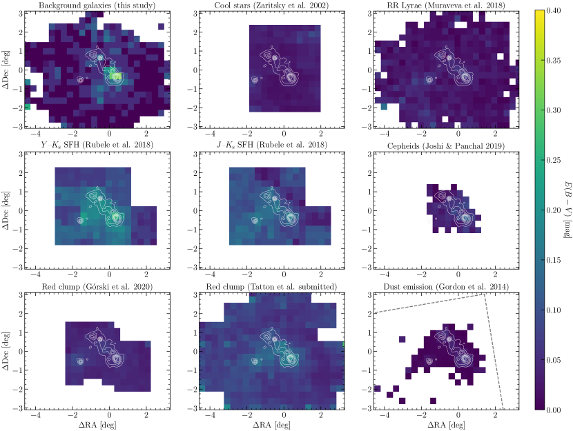
Figure 6: $20\times 20$ arcmin² resolution reddening maps covering the SMC. Each panel refers to a different literature source. The contours in all panels represent the IRAS 100 $\mu$m dust emission. The dashed line in the lower right panel represents the footprint of the HERITAGE observations.

Fig. 6 presents the comparison between our reddening map based on galaxies with low levels of intrinsic reddening and the various reddening maps of the SMC discussed in Section 4.1. To facilitate the comparison, we have resampled the literature maps to a $20\times 20$ arcmin² resolution by simply taking the median reddening value of all stars/cells that fall within a given bin. This resampling of the literature maps will undoubtedly result in the loss of small-scale (less than 20 arcmin in size) features in these maps. Any large-scale morphological features, however, such as pervasive enhancements of dust along the main body of the SMC, should be preserved and visible in the maps presented in Fig. 6.

Of the eight literature maps shown, three (Zaritsky et al., 2002, Muraveva et al., 2018 and Górski et al., 2020) show no obvious signs of enhanced levels of reddening associated with the main body of the SMC, when compared with the levels of reddening in regions away from the main body. In contrast, the remaining five maps (Gordon et al., 2014, the two realisations of Rubele et al., 2018, Joshi & Panchal, 2019 and Tatton et al. submitted) all exhibit clear signs of enhanced reddening in the south-western region of the main body ($\Delta$RA$\,\simeq$ 0.35, $\Delta$Dec$\,\simeq$ –0.35 deg) as well as other regions in some cases.

The presence of enhanced levels of dust appears to be tied to the type of star one uses to measure the reddening. The maps that show no significant levels of reddening across the SMC are all based on intermediate-age/old stars, whereas those that do show higher levels of intrinsic reddening (barring the Gordon et al., 2014 map) are either based on or include young stars. This difference in the reddening values based on old/young stellar populations can be ascribed to the spatial distribution of each population. The older stars are more uniformly distributed within the SMC as opposed to the young stars which tend to be concentrated in dense regions associated with recent star formation, i.e., their birth sites. Thus, in contrast to these young stars, the reddening values based on old stars will be more reflective of the diffuse interstellar medium (ISM) which, coupled with the averaging over spatial regions, means that dense regions with small filling factors will effectively be missed by the spatially averaged measurements from the older stars. Note that this effect is also observed in the two reddening maps presented by Zaritsky et al. (2002) based on the young, densely concentrated hot stars and the old, uniformly distributed cool stars.

Although the reddening maps based on older stellar populations tend to show very low levels of reddening across the SMC, the near-IR RC map of Tatton et al. (submitted) is a notable exception, despite the similar technique adopted to compute all RC reddening maps (see also Haschke et al., 2011; Górski et al., 2020). In Paper I (see section 5.2.2) we discussed some of the potential differences between the use of RC stars in the optical and near-IR regimes. The main difference between the maps shown in Fig. 6, however, is that Tatton et al. (submitted) determine reddening values for individual stars as opposed to for a discrete cell containing numerous stars. The use of cells as opposed to individual stars may act to hide small-scale features. We note that the region of enhanced intrinsic reddening in the Tatton et al. (submitted) map covers a significant fraction of the main body of the SMC and thus it is hard to reconcile why this is not somehow also an inherent feature of the published reddening maps inferred from the RC in the optical.

To place our comparison in a more quantitative context, we note that the median $E(B-V)$ value of our reddening map based on background galaxies with low levels of intrinsic reddening of $E(B-V)=0.05$ mag is consistent, to within the uncertainties, with the median values from all the literature reddening maps in Fig. 6. We find a minimum difference of $\Delta E(B-V)_{\mathrm{med}}=0.004$ mag in the comparison with the Górski et al. (2020) map, whereas a maximum difference of $\Delta E(B-V)_{\mathrm{med}}=-0.061$ mag is found in our comparison with the ($K_{\mathrm{s}},Y-K_{\mathrm{s}}$) Rubele et al. (2018) map. Note that we define $\Delta E(B-V)_{\mathrm{med}}$ as the median reddening of our map minus the median reddening of the literature map, such that positive values imply increased levels of reddening in our map and negative values increased levels of reddening in the relevant literature map. If we allow for the differences in the depth of the SMC sampled, we still find that the median reddening in all but the two realisations of the Rubele et al. (2018) reddening maps are consistent with the median value of our map. This is likely due to the extended regions of significant reddening observed in the Rubele et al. (2018) maps that cover a larger area of the SMC body than the regions of enhanced reddening in the other maps (see Fig. 6).

Our reddening map suggests that the highest levels of intrinsic reddening in the SMC are associated with the south-western region of the main body [$E(B-V)_{\mathrm{max}}=0.325$ mag]. Where observed, we check for consistency between the level of enhancement in our map compared to others in Fig. 6. A minimum difference of $\Delta E(B-V)=0.061$ mag is found for the ($K_{\mathrm{s}},Y-K_{\mathrm{s}}$) Rubele et al. (2018) map, whereas a maximum of $\Delta E(B-V)=0.205$ mag is found for the Joshi & Panchal (2019) map. For the maps that show no obvious enhancements of reddening in the main body, the differences are all larger than $\Delta E(B-V)=0.240$ mag. Despite the clumpy and inhomogeneous nature of dust in the SMC, that tends to be concentrated in and around star-forming regions, if we, for the sake of comparison, assume that the stars sample, on average, half the depth of the SMC, then by multiplying the reddening values of the stellar reddening maps by a factor of 2, we find that the enhancement observed in our reddening map based on background galaxies is consistent, to within the uncertainties, with the enhancements present in the Joshi & Panchal (2019), Tatton et al. (submitted) and the ($K_{\mathrm{s}},J-K_{\mathrm{s}}$) Rubele et al. (2018) maps [$\Delta E(B-V)=0.084$, $-0.060$ and $-0.026$ mag, respectively]. In contrast, the ($K_{\mathrm{s}},Y-K_{\mathrm{s}}$) Rubele et al. (2018) map implies significantly higher levels of reddening [$\Delta E(B-V)=-0.204$ mag] which is hard to reconcile with what we find using background galaxies. It is clear, however, that unlike the ($K_{\mathrm{s}},J-K_{\mathrm{s}}$) reddening map, there are strong tile-to-tile variations that could be due to issues pertaining to the absolute $Y$-band calibration of the VMC data (see Paper I).

Of the reddening maps shown in Fig. 6, perhaps the most like-for-like, in terms of sampling the full column density of dust along a given line of sight, is the HERITAGE dust map of Gordon et al. (2014). It is therefore interesting to note large discrepancies between that map and ours based on background galaxies. In terms of morphology, the Gordon et al. (2014) map suggests that the main body of the SMC has an enhanced level of reddening with respect to the outskirts. This level of enhancement, however, is significantly lower than what we observe in our map [cf. $E(B-V)_{\mathrm{med}}=0.008$ and $E(B-V)_{\mathrm{max}}=0.063$ mag for the Gordon et al., 2014 dust map with $E(B-V)_{\mathrm{med}}=0.050$ and $E(B-V)_{\mathrm{max}}=0.325$ mag for our reddening map]. Far-IR observations are excellent tracers of interstellar dust and the long wavelength coverage ($100-500$ $\mu$m) ensures an almost complete census of the dust mass of the SMC. Note that although a larger fraction of the dust luminosity is emitted at shorter mid- and near-IR wavelengths, these wavelengths only probe a small fraction of the total dust mass and thus their exclusion from the Gordon et al. (2014) analysis does not significantly affect the resultant reddening map shown in Fig. 6.

The main difference between the reddening maps based on background galaxies and the dust emission is that there are regions of high reddening in the former for which there is seemingly little emission in the latter. Although not obvious from Fig. 6 there is a difference in the dust emission associated with the south-western and north-eastern regions of the main body of the SMC, however these do not translate into the significant difference we observe in the galaxy-inferred reddening values. One possible reason for this discrepancy could be the spatial scales probed by the different tracers. The use of background galaxies provides the reddening within a very narrow column, whereas the spatial resolution of the images used to create the dust emission map are $\simeq$ 10 pc (having transformed the spatial resolution of all images to that of the 500 $\mu$m observations; see Gordon et al., 2014). Thus it is possible that the regions in the background galaxy reddening map with significant reddening could be due to dust clouds with very small spatial scales which are effectively missed by the far-IR observations.

Another potential cause for the discrepancy comes from the assumed far-IR emissivity used to convert the observed far-IR surface brightness into a dust surface density as well as the subsequent adopted value for $V$-band extinction efficiency factor, $Q_{V}$. Gordon et al. (2014) calibrate the far-IR emissivity using the far-IR/submillimetre SED of the diffuse MW ISM, however as noted by Roman-Duval et al. (2014, see their appendix A), the random error associated with this calibration translates to a systematic uncertainty on the dust surface density of 13 per cent. Furthermore, there is an additional systematic uncertainty of 22 per cent on the dust surface density related to the fact that the dust composition, and hence far-IR emissivity, in the MCs is not necessarily identical to that in the MW. Thus, the total systematic uncertainty on the derived dust surface density due to the poorly constrained nature of the far-IR emissivity (see also discussions in Fanciullo et al., 2015 and Clark et al., 2019) equates to 35 per cent. The extinction efficiency factor is a strong function of grain structure, composition and polarisation with studies indicating that variations in these can result in increases in the value of $Q_{V}$ by up to a factor of 3 (Gupta et al., 2005; Voshchinnikov, Il’in, & Henning, 2005). Given the uncertainties inherent in transforming far-IR dust emission observations into optical interstellar reddening values, and that to bring the reddening map based on dust emission into agreement with that inferred from background galaxies only requires a scaling of $\sim$ 5, it is not inconceivable that the two independent tracers could in fact provide consistent results.

The differences among reddening maps are likely highlighting interesting physical properties of the relative distributions of dust and stellar populations. The typical presumption of a smooth screen of dust is manifestly refuted by the different maps produced by young stars, old stars, and now galaxies. At first glance, it is puzzling that the two probes that are least likely to be spatially correlated with dust – old stars and galaxies – produce reddening maps that are in apparent disagreement. However, here we may be witnessing the effects of the third dimension. Stars are distributed along the line of sight relative to the dust and so some will be foreground to the dust, and hence unreddened, while others may lie behind the dust, and hence as reddened as background galaxies along the same line of sight. If the reddening and associated extinction along a line of sight is sufficiently strong to result in a bias in the stellar sample, then reddening values estimated using stars could be severely underestimated and result in apparent conflict in the maps from stars and from galaxies. Reddening estimates based on near-IR photometry may suffer less from such a bias, perhaps suggesting why the Tatton et al. (submitted) map is in better agreement with the galaxy-derived map. A complete treatment of this issue is beyond the scope of the current paper, but we do suggest an outline of a treatment where one begins with the galaxy-derived extinction map as the measurement of the full column-density of dust along the line of sight. Assuming that the dust is highly confined to the thin midplane, one could distribute stars in the foreground, within the midplane, and background. Within the midplane one would want to adjust the degree of correlation between stars and dust, particularly for the younger stars. By then mimicking the various sample selection effects and recreating the derived reddening maps, one could test whether the variety seen among reddening maps is reproduced and at the same time measure the relative distribution of stars and dust.

5 Summary

In this study we have extended the technique introduced in Paper I to quantify and map the total intrinsic reddening across $\simeq$ 34 deg² of the SMC based on the analysis of SEDs of background galaxies. Below we provide a brief overview of the steps involved and our main conclusions.

1. We use a combination of colour–magnitude and morphological selections to select an initial sample of $\sim$ 500,000 likely background sources from the VMC PSF photometric catalogues covering the combined SMASH-VMC footprint of the SMC. We consistently measure fluxes for each source using lambdar and create SEDs from the optical ($ugriz$; SMASH) and near-IR ($YJK_{\mathrm{s}}$; VMC) broadband images

2. We use the lephare $\chi^{2}$ template-fitting code to fit a combination of galaxy, QSO and stellar templates to the SEDs. From these, we select a cleaned subsample of 29,274 galaxies with low levels of intrinsic reddening to create an intrinsic reddening map of the SMC. Our reddening map shows statistically significant levels of enhanced reddening associated with the main body of the SMC compared with negligible levels of reddening in the outskirts [$\Delta E(B-V)\simeq 0.3$ mag].

3. We find very good agreement between the calculated lephare photometric redshifts and the spectroscopically determined redshifts for a sample of 46 QSOs behind the SMC (median $\Delta z=-0.006$).

4. We perform a comparison of our intrinsic reddening map with publicly available reddening maps of the SMC. As noted in Paper I, there is significant variation amongst the various literature maps that tends to be dependent upon the adopted tracer. Having accounted for the difference in the SMC depth probed using stellar tracers and background galaxies, we find that the levels of enhanced reddening observed in reddening maps that include contributions from young stars is consistent with the levels of enhancement we observe in our reddening map. For reddening maps based on older stellar populations we find a significant discrepancy between the levels of reddening associated with the main body of the SMC. One notable exception to this is the near-IR RC map of Tatton et al. (submitted) that is consistent with our findings. Our comparison with the HERITAGE dust map of Gordon et al. (2014) also shows a significant discrepancy, however this could be due to the different length scales probed by the respective tracers as well as uncertainties in the far-IR emissivity and the optical properties of the dust grains.

5. In a future work we aim to use publicly available reddening maps of the SMC to test the inferred dust densities by comparing these to the expected limits on the gas-to-dust ratio to potentially highlight unrealistic dust mass densities (i.e. high reddening values; see e.g. Gordon et al., 2014; Roman-Duval et al., 2014).

Data Availability

The data underlying this article are available in the article and in its online supplementary material. The SMASH and VMC survey images used to create the galaxy SEDs are publicly available at https://datalab.noao.edu/smash/smash.php#SecondtDataRelease and https://www.eso.org/sci/publications/announcements/sciann17313.html, respectively. The galaxy SEDs will be shared on reasonable request to the corresponding author.

References

- Arnouts et al. (2007) Arnouts S., Walcher C. J., Le Fèvre O., et al., 2007, A&A, 476, 137
- Bailey et al. (2015) Bailey M., van Loon J. T., Sarre P. J., Beckman J. E., 2015, MNRAS, 454, 4013
- Bell et al. (2019) Bell C. P. M., Cioni M.-R. L., Wright A. H., et al., 2019, MNRAS, 489, 3200
- Bolatto et al. (2007) Bolatto A. D., Simon J. D., Stanimirović S., van Loon J. T., Shah R. Y., Venn K., Leroy A. K., Sandstrom K., Jackson J. M., Israel F. P., Li A., Staveley-Smith L., Bot C., Boulanger F., Rubio M., 2007, ApJ, 655, 212
- Bouchet et al. (1985) Bouchet P., Lequeux J., Maurice E., Prevot L., Prevot-Burnichon M. L., 1985, A&A, 149, 330
- Cardelli et al. (1989) Cardelli J. A., Clayton G. C., Mathis J. S., 1989, ApJ, 345, 245
- Chlewicki (1985) Chlewicki G., 1985, PhD thesis, Observational Constraints on Multimodal Interstellar Grain Populations (Leiden University)
- Choi et al. (2018) Choi Y., Nidever D. L., Olsen K., et al., 2018, ApJ, 866, 90
- Cioni et al. (2011) Cioni M.-R. L., Clementini G., Girardi L., et al., 2011, A&A, 527, A116
- Clark et al. (2019) Clark C. J. R., De Vis P., Baes M., Bianchi S., Casasola V., Cassarà L. P., Davies J. I., Dobbels W., Lianou S., De Looze I., Evans R., Galametz M., Galliano F., Jones A. P., Madden S. C., Mosenkov A. V., Verstocken S., Viaene S., Xilouris E. M., Ysard N., 2019, MNRAS, 489, 5256
- Dahlen et al. (2013) Dahlen T., Mobasher B., Faber S. M., et al., 2013, ApJ, 775, 93
- de Grijs & Bono (2015) de Grijs R., Bono G., 2015, AJ, 149, 179
- de Grijs et al. (2014) de Grijs R., Wicker J. E., Bono G., 2014, AJ, 147, 122
- Dobrzycki et al. (2003a) Dobrzycki A., Macri L. M., Stanek K. Z., Groot P. J., 2003a, AJ, 125, 1330
- Dobrzycki et al. (2003b) Dobrzycki A., Stanek K. Z., Macri L. M., Groot P. J., 2003b, AJ, 126, 734
- El Youssoufi et al. (2019) El Youssoufi D., Cioni M.-R. L., Bell C. P. M., Rubele S., Bekki K., de Grijs R., Girardi L., Ivanov V. D., Matijevic G., Niederhofer F., Oliveira J. M., Ripepi V., Subramanian S., van Loon J. T., 2019, MNRAS, 490, 1076
- Fanciullo et al. (2015) Fanciullo L., Guillet V., Aniano G., Jones A. P., Ysard N., Miville-Deschênes M. A., Boulanger F., Köhler M., 2015, A&A, 580, A136
- Freedman et al. (2020) Freedman W. L., Madore B. F., Hoyt T., Jang I. S., Beaton R., Lee M. G., Monson A., Neeley J., Rich J., 2020, ApJ, 891, 57
- Geha et al. (2003) Geha M., Alcock C., Allsman R. A., et al., 2003, AJ, 125, 1
- Gieren et al. (2018) Gieren W., Storm J., Konorski P., Górski M., Pilecki B., Thompson I., Pietrzyński G., Graczyk D., Barnes T. G., Fouqué P., Nardetto N., Gallenne A., Karczmarek P., Suchomska K., Wielgórski P., Taormina M., Zgirski B., 2018, A&A, 620, A99
- Gordon et al. (2014) Gordon K. D., Roman-Duval J., Bot C., et al., 2014, ApJ, 797, 85
- Górski et al. (2020) Górski M., Zgirski B., Pietrzyński G., Gieren W., Wielgórski P., Graczyk D., Kudritzki R.-P., Pilecki B., Narloch W., Karczmarek P., Suchomska K., Taormina M., 2020, ApJ, 889, 179
- Gouliermis et al. (2014) Gouliermis D. A., Hony S., Klessen R. S., 2014, MNRAS, 439, 3775
- Groenewegen (2018) Groenewegen M. A. T., 2018, A&A, 619, A8
- Gupta et al. (2005) Gupta R., Mukai T., Vaidya D. B., Sen A. K., Okada Y., 2005, A&A, 441, 555
- Haschke et al. (2011) Haschke R., Grebel E. K., Duffau S., 2011, AJ, 141, 158
- Hunter (2007) Hunter J. D., 2007, Computing in Science & Engineering, 9, 90
- Ilbert et al. (2009) Ilbert O., Capak P., Salvato M., et al., 2009, ApJ, 690, 1236
- Ilbert et al. (2013) Ilbert O., McCracken H. J., Le Fèvre O., et al., 2013, A&A, 556, A55
- Ivanov et al. (2016) Ivanov V. D., Cioni M.-R. L., Bekki K., de Grijs R., Emerson J., Gibson B. K., Kamath D., van Loon J. T., Piatti A. E., For B.-Q., 2016, A&A, 588, A93
- Jarvis et al. (2013) Jarvis M. J., Bonfield D. G., Bruce V. A., et al., 2013, MNRAS, 428, 1281
- Jones et al. (2001–) Jones E., Oliphant T. E., Peterson P., et al., 2001–, SciPy: Open source scientific tools for Python
- Joshi & Panchal (2019) Joshi Y. C., Panchal A., 2019, A&A, 628, A51
- Kohout et al. (2014) Kohout T., Kallonen A., Suuronen J. P., Rochette P., Hutzler A., Gattacceca J., Badjukov D. D., Skála R., Böhmová V., Čuda J., 2014, Meteoritics and Planetary Science, 49, 1157
- Kozłowski et al. (2011) Kozłowski S., Kochanek C. S., Udalski A., 2011, ApJS, 194, 22
- Kozłowski et al. (2013) Kozłowski S., Onken C. A., Kochanek C. S., Udalski A., Szymański M. K., Kubiak M., Pietrzyński G., Soszyński I., Wyrzykowski Ł., Ulaczyk K., Poleski R., Pietrukowicz P., Skowron J., OGLE Collaboration, Meixner M., Bonanos A. Z., 2013, ApJ, 775, 92
- Le Fèvre et al. (2005) Le Fèvre O., Vettolani G., Garilli B., et al., 2005, A&A, 439, 845
- Maitra et al. (2019) Maitra C., Haberl F., Ivanov V. D., Cioni M.-R. L., van Loon J. T., 2019, A&A, 622, A29
- Mann & Kimura (2000) Mann I., Kimura H., 2000, J. Geophys. Res., 105, 10317
- McKinney (2010) McKinney W., 2010, in Proceedings of the 9th Python in Science Conference, van der Walt S., Millman J., eds., p. 51
- Meixner et al. (2013) Meixner M., Panuzzo P., Roman-Duval J., et al., 2013, AJ, 146, 62
- Muller et al. (2003) Muller E., Staveley-Smith L., Zealey W., Stanimirović S., 2003, MNRAS, 339, 105
- Muraveva et al. (2018) Muraveva T., Subramanian S., Clementini G., Cioni M.-R. L., Palmer M., van Loon J. T., Moretti M. I., de Grijs R., Molinaro R., Ripepi V., Marconi M., Emerson J., Ivanov V. D., 2018, MNRAS, 473, 3131
- Nayak et al. (2018) Nayak P. K., Subramaniam A., Choudhury S., Sagar R., 2018, A&A, 616, A187
- Nidever et al. (2017) Nidever D. L., Olsen K., Walker A. R., et al., 2017, AJ, 154, 199
- Oliphant (2015) Oliphant T. E., 2015, Guide to NumPy. CreateSpace Independent Publishing Platform, 2nd ed.
- Paturel et al. (2003) Paturel G., Petit C., Prugniel P., Theureau G., Rousseau J., Brouty M., Dubois P., Cambrésy L., 2003, A&A, 412, 45
- Prevot et al. (1984) Prevot M. L., Lequeux J., Prevot L., Maurice E., Rocca-Volmerange B., 1984, A&A, 132, 389
- Riess et al. (2019) Riess A. G., Casertano S., Yuan W., Macri L. M., Scolnic D., 2019, ApJ, 876, 85
- Riess et al. (2009) Riess A. G., Macri L., Casertano S., Sosey M., Lampeitl H., Ferguson H. C., Filippenko A. V., Jha S. W., Li W., Chornock R., Sarkar D., 2009, ApJ, 699, 539
- Ripepi et al. (2017) Ripepi V., Cioni M.-R. L., Moretti M. I., et al., 2017, MNRAS, 472, 808
- Ripepi et al. (2019) Ripepi V., Molinaro R., Musella I., Marconi M., Leccia S., Eyer L., 2019, A&A, 625, A14
- Roman-Duval et al. (2014) Roman-Duval J., Gordon K. D., Meixner M., et al., 2014, ApJ, 797, 86
- Rubele et al. (2015) Rubele S., Girardi L., Kerber L., Cioni M.-R. L., Piatti A. E., Zaggia S., Bekki K., Bressan A., Clementini G., de Grijs R., Emerson J. P., Groenewegen M. A. T., Ivanov V. D., Marconi M., Marigo P., Moretti M.-I., Ripepi V., Subramanian S., Tatton B. L., van Loon J. T., 2015, MNRAS, 449, 639
- Rubele et al. (2018) Rubele S., Pastorelli G., Girardi L., Cioni M.-R. L., Zaggia S., Marigo P., Bekki K., Bressan A., Clementini G., de Grijs R., Emerson J., Groenewegen M. A. T., Ivanov V. D., Muraveva T., Nanni A., Oliveira J. M., Ripepi V., Sun N.-C., van Loon J. T., 2018, MNRAS, 478, 5017
- Sandstrom et al. (2010) Sandstrom K. M., Bolatto A. D., Draine B. T., Bot C., Stanimirović S., 2010, ApJ, 715, 701
- Smartt et al. (2015) Smartt S. J., Valenti S., Fraser M., et al., 2015, A&A, 579, A40
- Stanimirović et al. (1999) Stanimirović S., Staveley-Smith L., Dickey J. M., Sault R. J., Snowden S. L., 1999, MNRAS, 302, 417
- Taylor (2005) Taylor M. B., 2005, in Astronomical Society of the Pacific Conference Series, Vol. 347, Astronomical Data Analysis Software and Systems XIV, Shopbell P., Britton M., Ebert R., eds., p. 29
- The Astropy Collaboration et al. (2018) The Astropy Collaboration, Price-Whelan A. M., Sipőcz B. M., Günther H. M., et al., 2018, AJ, 156, 123
- Udalski (2003) Udalski A., 2003, Acta Astron., 53, 291
- Udalski et al. (2015) Udalski A., Szymański M. K., Szymański G., 2015, Acta Astron., 65, 1
- Véron-Cetty & Véron (2010) Véron-Cetty M.-P., Véron P., 2010, A&A, 518, A10
- Voshchinnikov et al. (2005) Voshchinnikov N. V., Il’in V. B., Henning T., 2005, A&A, 429, 371
- Whittet (2003) Whittet D. C. B., 2003, Dust in the Galactic Environment. Bristol: Institute of Physics Publishing, 2nd ed.
- Wright et al. (2016) Wright A. H., Robotham A. S. G., Bourne N., et al., 2016, MNRAS, 460, 765
- Zaritsky et al. (2002) Zaritsky D., Harris J., Thompson I. B., Grebel E. K., Massey P., 2002, AJ, 123, 855
- Zivkov et al. (2018) Zivkov V., Oliveira J. M., Petr-Gotzens M. G., Cioni M.-R. L., Rubele S., van Loon J. T., Bekki K., Cusano F., de Grijs R., Ivanov V. D., Marconi M., Niederhofer F., Ripepi V., Sun N.-C., 2018, A&A, 620, A143